1 Introduction
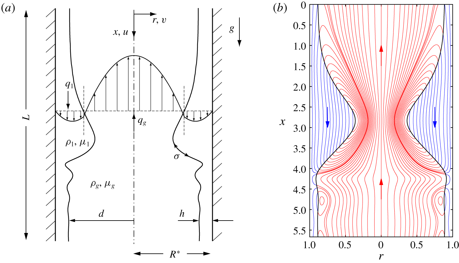
We consider the configuration in figure 1, a thin liquid film falling down the inner surface of a vertical cylindrical tube of radius  $R^{\star }$ under the action of the gravitational acceleration
 $g$. The film of liquid (denoted with the subscript
 $l$) is in contact with a laminar flow of gas in the core (subscript
 $g$). Both fluids are assumed to be Newtonian with constant densities
 $\unicode[STIX]{x1D70C}_{l}$ and
 $\unicode[STIX]{x1D70C}_{g}$, dynamic viscosities
 $\unicode[STIX]{x1D707}_{l}$ and
 $\unicode[STIX]{x1D707}_{g}$, and surface tension
 $\unicode[STIX]{x1D70E}$. Also, we assume the arrangement to be axisymmetric. We denote the film thickness
 $h$, the core radius
 $d$, its spatial average
 $\bar{d}$ and the flow rates
 $q_{l}$ and
 $q_{g}$. Their dimensional counterparts will be distinguished by a star, e.g.
 $d^{\star }$, and their counterparts in the corresponding flat-film primary flow will be denoted with a subscript zero, e.g.
 $d_{0}$.
We focus on conditions, where: (i) the effect of gravity, quantified through the Bond number  $Bo=\unicode[STIX]{x1D70C}_{l}gR^{\star 2}/\unicode[STIX]{x1D70E}$, is at least comparable to that of capillarity (
 $Bo\geqslant 1$); (ii) the liquid film’s inertia, quantified through the Reynolds number
 $Re=q_{l0}^{\star }\unicode[STIX]{x1D70C}_{l}/(\unicode[STIX]{x03C0}R^{\star }\unicode[STIX]{x1D707}_{l})$, is not necessarily negligible (
 $Re\leqslant 20$); and (iii) the effect of the gas flow can be relevant, but its Reynolds number
 $Re_{g}=q_{g0}^{\star }\unicode[STIX]{x1D70C}_{g}/(\unicode[STIX]{x03C0}R^{\star }\unicode[STIX]{x1D707}_{g})$ remains moderate (
 $|Re_{g}|<20$).
Falling liquid film (subscript  $l$) lining the inner surface of a narrow cylindrical tube in contact with a laminar gas flow in the core (subscript
 $g$). (a) Problem configuration and notations. The tube radius
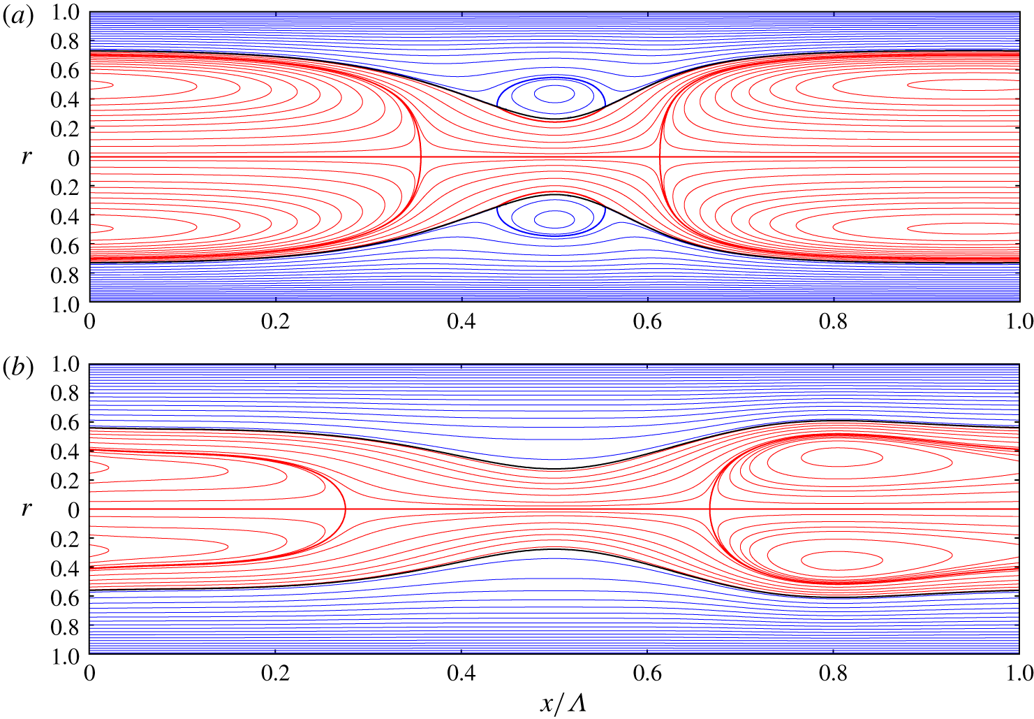
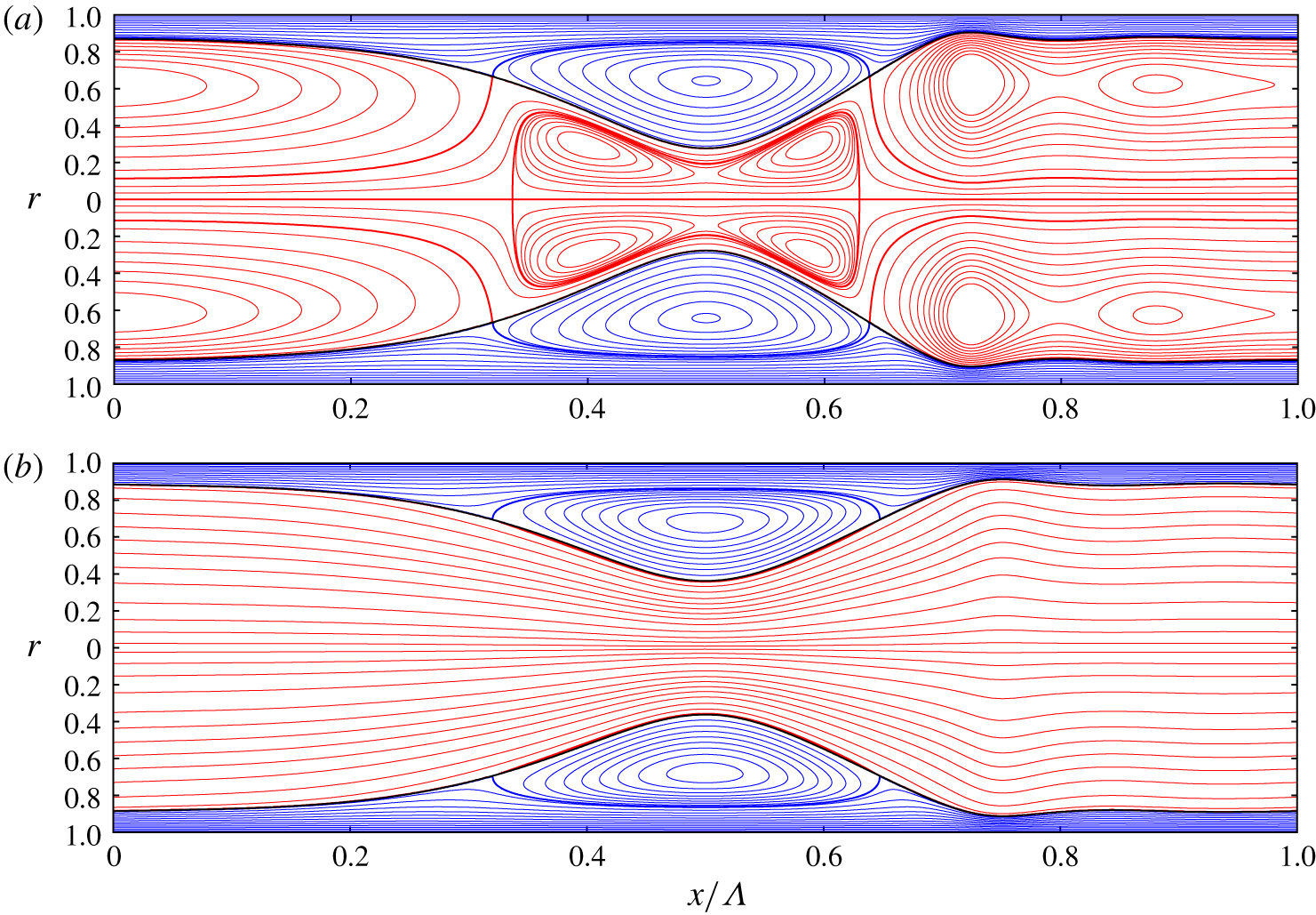
 $R^{\star }$ is the length scale, the star superscript designating dimensional quantities. (b) Example of a travelling-wave computation with our model (2.5): case 4 in table 1 (low-viscosity silicone oil),
 $Re=14.6$,
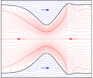
 $Re_{g}=-17.27$ (limit point marked by an asterisk in figure 13a). Streamlines in the wall-fixed reference frame within the liquid (blue lines) and gas (red lines).

We investigate this flow with the weighted residual integral boundary layer (WRIBL) model of Dietze & Ruyer-Quil (Reference Dietze and Ruyer-Quil2015), which was previously applied only to gravity-free films. The model accounts for gravity, inertia, full interfacial curvature, axial viscous diffusion and full inter-phase coupling. Our model computations are confronted with our own direct numerical simulations (DNS) in appendix A and figure 5(d).
We focus on the occlusion of the narrow tube due to the interfacial instability of the falling liquid film, as observed experimentally by Dao & Balakotaiah (Reference Dao and Balakotaiah2000) and Camassa, Ogrosky & Olander (Reference Camassa, Ogrosky and Olander2014). Occlusion is relevant for chemical engineering applications such as tubular falling film micro-reactors (Seebauer et al. Reference Seebauer, Poechlauer, Braune and Steinhofer2012). It also occurs in the human pulmonary airways due to the collapse of the mucus-serous film lining their inner surface (Grotberg Reference Grotberg2011). In the lower generations of bronchioles, the effect of gravity and possibly inertia is not necessarily negligible (Kamm & Schroter Reference Kamm and Schroter1989).
The falling liquid film is subject to two instability mechanisms causing interfacial deformations: the Plateau–Rayleigh mechanism (Plateau Reference Plateau1849; Rayleigh 1892; Goren Reference Goren1962), due to the azimuthal curvature of the film surface; and the Kapitza mechanism (Kapitza Reference Kapitza1948), due to inertia, which sets in as a result of the gravity-driven mean flow (Brooke Benjamin Reference Brooke Benjamin1957; Yih Reference Yih1963). The strength of this mean flow determines whether the absolute nature of the Plateau–Rayleigh instability or the convective nature of the Kapitza instability dominates (Duprat et al. Reference Duprat, Ruyer-Quil, Kalliadasis and Giorgiutti-Dauphiné2007). For the liquids studied here, we find that occlusion is dictated by absolute instability when  $Bo\ll 1$, whereas convective instability is responsible for occlusion when
 $Bo\geqslant 1$.
In the case of convective instability, the liquid film can produce travelling surface waves, which remain stationary in their reference frame. Gravity plays an important role in shaping these waves, compressing the leading and elongating the trailing wave front, which results in asymmetric tear-shaped wave humps (Dietze Reference Dietze2016). The resulting distortion of the film surface favours variations in axial (stabilizing) over azimuthal (destabilizing) surface curvature. In related systems, this mechanism has been found to saturate the Plateau–Rayleigh instability in the weakly nonlinear regime (Frenkel et al. Reference Frenkel, Babchin, Levich, Shlang and Sivashinsky1987), to the extent that the film looks stable to the naked eye (Quéré Reference Quéré1990). In our current problem, we find that it greatly extends the region of existence of strongly nonlinear travelling waves and considerably delays occlusion.
Trifonov (Reference Trifonov1992) applied the integral boundary layer approach of Shkadov (Reference Shkadov1967) to model an annular liquid film falling in a vertical cylindrical tube. The author found that the Plateau–Rayleigh mechanism systematically increases the amplitude of travelling waves versus a planar falling liquid film, where only the Kapitza mechanism is active. He also observed catastrophic growth, when the amplitude of travelling-wave solutions diverged as a function of  $1/R$. In those instances, the effect of gravity was negligible, i.e.
 $Bo\ll 1$. By contrast, we focus on occlusion in the limit
 $Bo\geqslant 1$. Moreover, the model of Trifonov (Reference Trifonov1992) did not account for axial viscous diffusion, which we find to greatly precipitate occlusion in high-viscosity films.
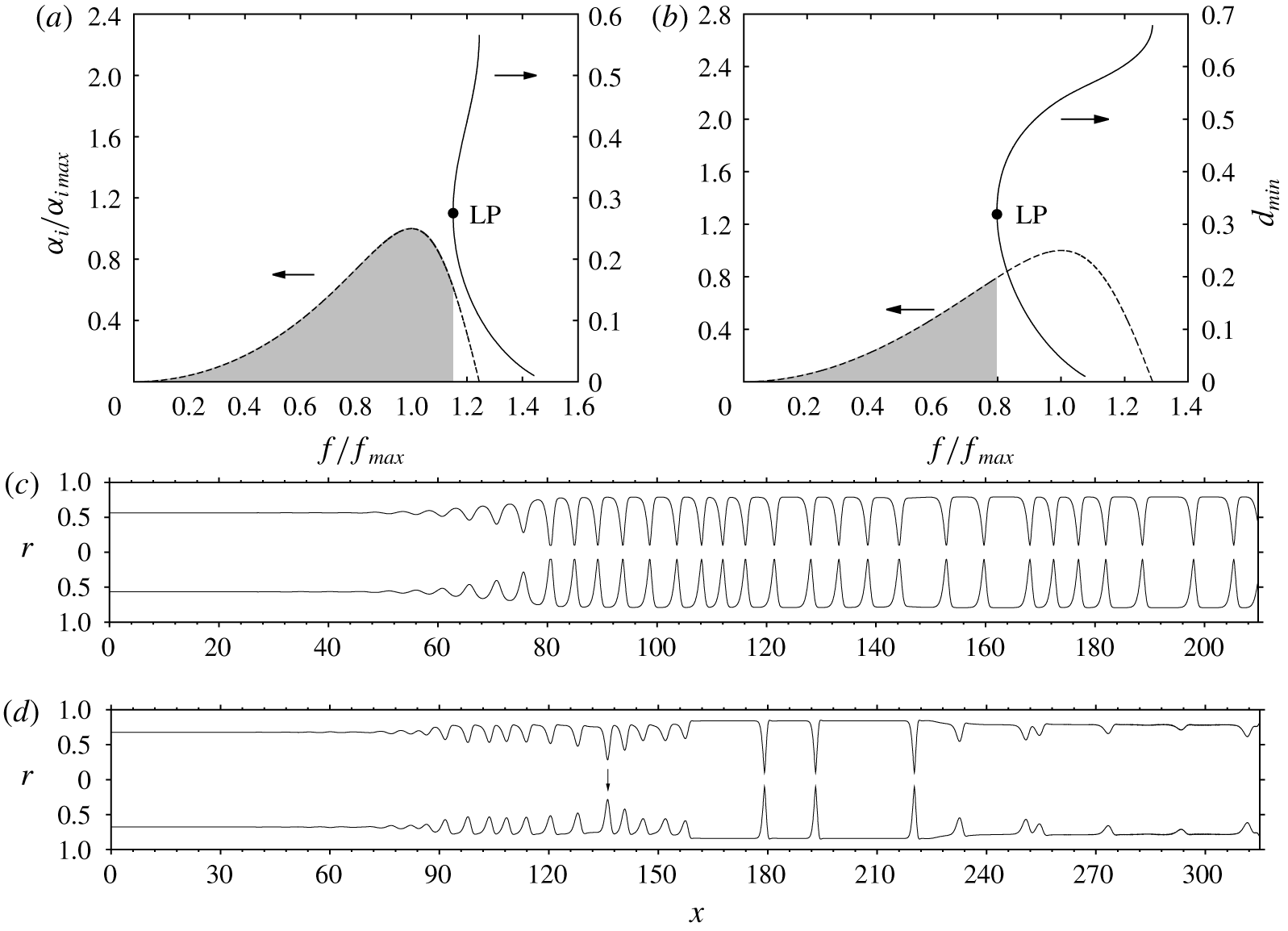
Dao & Balakotaiah (Reference Dao and Balakotaiah2000) performed falling-film experiments in long narrow tubes and determined the occlusion onset in terms of  $Re$ for a wide range of liquids. However, no information was available on the wave dynamics responsible for occlusion. By reproducing two of these experiments (runs 13 and 20 there) with our own spatio-temporal computations, we provide this missing information, leading us to distinguish two wave-induced occlusion scenarios. In scenario I, waves causing occlusion emerge directly from linear wave selection. In scenario II, they result from the secondary instability of a regular train of travelling waves, triggering a cascade of coalescence/absorption events that produce increasingly long, more dangerous, waves. The secondary instability (Liu & Gollub Reference Liu and Gollub1993) and the ensuing cascaded coarsening dynamics (Chang et al. Reference Chang, Demekhin, Kalaidin and Ye1996b) are well-known phenomena in planar falling liquid films.
Jensen (Reference Jensen2000) investigated annular collars travelling on a gravity-driven liquid film lining the inner surface of a cylindrical tube. The collars were constructed from unduloids, i.e. symmetric constant-curvature equilibrium shapes (Delaunay Reference Delaunay1841). The author studied under what conditions collars may grow to occlude the tube. Our study extends this work in that the collar shape is not forced to be symmetric, but follows implicitly from the evolution equations. This allows for the gravity-induced distortion of collars, which we find can greatly delay occlusion.
Camassa et al. (Reference Camassa, Ogrosky and Olander2014) performed falling-film occlusion experiments in a transparent tube, using a high-viscosity silicone oil. By confronting these with linear stability calculations, the authors concluded that occlusion is caused by spatially growing nonlinear waves and not by absolute linear instability ( $Bo=11.06$ in their experiments). Furthermore, with the help of a first-order long-wave model obtained from asymptotic expansion (Benney Reference Benney1966), the authors constructed travelling-wave solutions. By continuing these at fixed wavelength in terms of
 $Re$, they identified a limit point, and conjectured that this may signal the occlusion onset in a real system. However, the authors cautioned that further work was needed to verify this with respect to their experiments. This work was initiated by Camassa et al. (Reference Camassa, Marzuola, Ogrosky and Vaughn2016), but their model did not account for axial viscous diffusion, which we show to strongly affect travelling-wave solutions, and the wavelength assumed in their continuation was too long compared to the experiment.
In our current study, we have checked the conjecture of Camassa et al. (Reference Camassa, Ogrosky and Olander2014) based on travelling-wave and spatio-temporal computations with our model. We have successfully confronted these computations with the experiments of Camassa et al. (Reference Camassa, Ogrosky and Olander2014) and find that accounting for axial viscous diffusion greatly improves agreement. Based on our computations, we find that the surface waves causing occlusion indeed systematically lie beyond the limit of travelling-wave solutions (figure 4), confirming the conjecture of Camassa et al. (Reference Camassa, Ogrosky and Olander2014). This limit is highly sensitive to the considered wavelength, long waves being more dangerous than short waves, as shown by Camassa et al. (Reference Camassa, Marzuola, Ogrosky and Vaughn2016) and Ding et al. (Reference Ding, Liu, Liu and Yang2019). Thus, any predictive criterion for occlusion based on travelling-wave solutions must account for the type of waves that actually occur in a real system.
For this, we introduce the upper conservative occlusion bound  $Re_{max}$, which corresponds to the limit point of travelling-wave solutions at the spatially most amplified frequency of linear waves
 $f_{max}$. For
 $Re>Re_{max}$, the most amplified surface waves, which typically emerge in an experiment, do not possess travelling states and occlusion is certain to occur in a naturally evolving film. We find that the occlusion experiments of Camassa et al. (Reference Camassa, Ogrosky and Olander2014) and experimental run 20 in Dao & Balakotaiah (Reference Dao and Balakotaiah2000) correspond to this regime. Occlusion in this case occurs through scenario I. To determine
 $Re_{max}$ we have computed the most amplified wave frequency
 $f_{max}$ in our numerical continuations by solving the linear spatial stability problem along with our nonlinear model equations. This had not been attempted by Camassa et al. (Reference Camassa, Ogrosky and Olander2014) and Ding et al. (Reference Ding, Liu, Liu and Yang2019).
At the other end, occlusion is delimited by a lower conservative bound  $Re=Re_{0}$, below which travelling-wave solutions always exist, no matter how great the wavelength, and occlusion is impossible. The existence of such a limit was discovered by Ding et al. (Reference Ding, Liu, Liu and Yang2019).
We find that the conservative occlusion bounds  $Re_{0}$ and
 $Re_{max}$ delimit a region of conditional occlusion,
 $Re_{0}<Re<Re_{max}$, where occlusion is theoretically possible (for long enough waves) but does not necessarily occur in a real system. Whether it does, depends on the specific wave dynamics that unfold over the spatio-temporal evolution of the film, and whether the tube is long enough to accommodate this. In this regime, we find that occlusion is caused by scenario II and that it applies to experimental run 13 in Dao & Balakotaiah (Reference Dao and Balakotaiah2000). It also opens the possibility of preventing occlusion through coherent inlet forcing, i.e. by forcing waves of sufficiently high frequency. We validate this idea based on spatio-temporal computations.
Unless  $Bo$ is very large, we find that the height of the travelling waves at the limit point
 $Re=Re_{max}$ is far from reaching the tube radius. In contrast to what Dao & Balakotaiah (Reference Dao and Balakotaiah2000) conjectured, travelling-wave solutions are thus lost abruptly and not due to the wave height reaching the tube radius continuously.
Zhou et al. (Reference Zhou, Peng, Zhang and Zhuge2016) investigated viscoelastic liquid films falling in a deformable narrow tube. The authors performed calculations with a model based on the same approach as Trifonov (Reference Trifonov1992), which does not account for axial viscous diffusion. Interestingly, it was shown that occlusion can cause a contraction of the flexible tube. Such events are known to occur in the pulmonary airways (Grotberg Reference Grotberg2011) and can damage cells within the capillaries (Bian et al. Reference Bian, Tai, Halpern, Zheng and Grotberg2010). The authors went on to determine the occlusion onset by varying the liquid flow rate in spatio-temporal computations. This onset was defined as the point at which the computation breaks down due to an occlusion event. However, such computations cannot attain a representative developed state. For example, when starting from a flat-film initial condition, a single unrealistically large tsunami-like wave usually develops in the early stages. This wave is bound to cause occlusion, but it is not representative of a real system. By contrast, we characterize occlusion based on the bounds  $Re_{0}$ and
 $Re_{max}$ of travelling-wave solutions, and our spatio-temporal computations have all been continued until reaching a statistically developed state. To achieve this, we have allowed our computations to continue past occlusion events by numerically limiting the core radius of an occluded region to a small but finite value.
Liu & Ding (Reference Liu and Ding2017) studied a vertically falling glycerol film flowing down a porous cylindrical surface using a lubrication equation. The authors found that porosity precipitates both the absolute instability threshold and the occlusion limit. Using the same approach, Ding et al. (Reference Ding, Liu, Liu and Yang2019) studied the effect of the Marangoni instability on a radially heated liquid film falling in a vertical cylindrical tube. The authors found that Marangoni stresses promote/delay occlusion when the film is heated/cooled from the wall. However, their modelling approach does not account for inertia nor axial viscous diffusion. We find that this does not allow us to accurately predict occlusion in high-viscosity (because of axial viscous diffusion) or low-viscosity (because of inertia) liquids.
The model employed in our current study extends upon the earlier works of Trifonov (Reference Trifonov1992), Camassa et al. (Reference Camassa, Ogrosky and Olander2014), Camassa, Ogrosky & Olander (Reference Camassa, Ogrosky and Olander2017), Zhou et al. (Reference Zhou, Peng, Zhang and Zhuge2016), Liu & Ding (Reference Liu and Ding2017) and Ding et al. (Reference Ding, Liu, Liu and Yang2019) by accounting for axial viscous diffusion and inertia. This has allowed us to investigate four real liquids, for which we determine the lower and upper occlusion bounds  $Re_{0}$ and
 $Re_{max}$ and characterize the possible occlusion scenarios. When the viscosity is high, we find that axial viscous diffusion greatly precipitates the upper occlusion bound
 $Re_{max}$ (by 74 % for the high-viscosity silicone oil). When the viscosity is low (low-viscosity silicone oil), inertia cannot be neglected and is found to precipitate
 $Re_{max}$ by 20 %. We also find that these two effects determine whether the occlusion mechanism is dictated by absolute linear instability or the loss of travelling-wave solutions.
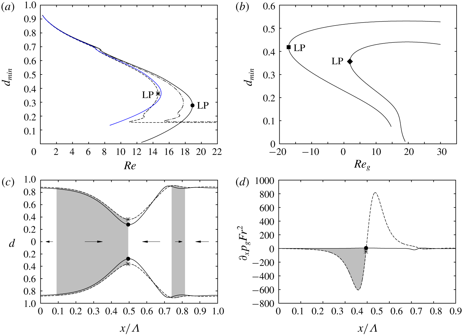
Our model also accounts for full inter-phase coupling between the liquid and gas, and this has allowed us to study the effect of a laminar counter-current gas flow on the occlusion bound  $Re_{max}$. For low-viscosity liquids, where the wave-induced pressure variation in the gas becomes relevant in the liquid force balance, we find that
 $Re_{max}$ is significantly reduced with increasing
 $|Re_{g}|$ (by up to 25 % in our computations). Thereby, the conditions we have studied differ from previous works. Alekseenko et al. (Reference Alekseenko, Aktershev, Cherdantsev, Kharlamov and Markovich2009) experimentally studied the linear stability of a falling liquid film subject to a co-current turbulent gas flow. Their tube radius was large and thus occlusion could not occur. Camassa et al. (Reference Camassa, Forest, Lee, Ogrosky and Olander2012, Reference Camassa, Ogrosky and Olander2017) studied co-current upward liquid/gas flows based on a long-wave model, where the effect of the (turbulent) gas flow was accounted for by relaxing the inter-phase coupling conditions in the limit of high gas velocities. By contrast, we focus on laminar (counter-current) gas flows, where our model, which relies on the unrelaxed coupling conditions, behaves well.
For the case of a planar falling liquid film sheared by a confined gas flow, many works have investigated the flooding phenomenon, where the liquid film either occludes the channel (Vlachos et al. Reference Vlachos, Paras, Mouza and Karabelas2001), surface waves (Tseluiko & Kalliadasis Reference Tseluiko and Kalliadasis2011) or the liquid flow (Trifonov Reference Trifonov2010) reverse direction, or the liquid film disintegrates into drops (Zapke & Kröger Reference Zapke and Kröger2000).
Finally, several works are related less directly to the studied problem. Kouris & Tsamopoulos (Reference Kouris and Tsamopoulos2001) studied liquid/liquid gravity-driven flows through a vertical pipe. Beltrame (Reference Beltrame2018) studied the transition between partial and complete wetting in a microtube. Xu & Jensen (Reference Xu and Jensen2017) studied migration of liquid films in tubes with rough walls. Moreover, many works have dealt with pressure-driven core-annular flows (Aul & Olbricht Reference Aul and Olbricht1990; Joseph, Chen & Renardy Reference Joseph, Chen and Renardy1997) or liquid films falling down fibres (Kalliadasis & Chang Reference Kalliadasis and Chang1994; Quéré Reference Quéré1999). In the latter case, occlusion cannot occur, unless the gas phase is confined by an additional concentric hollow cylinder (Wray Reference Wray2013).
Our manuscript is structured as follows. In section 2 we introduce the governing equations, and details of our model (§ 2.1), direct numerical simulations (§ 2.2) and linear stability calculations (§ 2.3). Results are presented in § 3, where we start by proving that occlusion in real systems results from surface waves that lie beyond the limit of travelling-wave solutions (§ 3.1). In § 3.2 we compute the upper and lower occlusion bounds  $Re_{max}$ and
 $Re_{0}$, delimiting the regimes of certain, conditional, and impossible occlusion. For one of the studied cases, we validate these results based on our own DNS of travelling-wave solutions. In §§ 3.3 to 3.6 we show how
 $Re_{max}$ is affected by gravity, axial viscous diffusion, inertia and the core gas flow. In § 3.7 we demonstrate occlusion scenarios I (certain occlusion regime) and II (conditional occlusion regime) by reproducing two of the experimental runs from Dao & Balakotaiah (Reference Dao and Balakotaiah2000) with spatio-temporal computations. In § 3.8 we show that occlusion in the conditional regime can be prevented through coherent inlet forcing. Conclusions are drawn in § 4. The appendix reports comparisons with transient DNS (appendix A), numerical details regarding our travelling-wave DNS (appendix B), as well as additional discussions of figures 13(a) (appendix C) and 4(a) (appendix D). Finally, in appendix E we introduce an augmented version of our WRIBL model that allows a better representation of liquid plugs, based on a localized force term.
2 Mathematical description
We consider the flow in figure 1(a), which is rotationally symmetric with respect to the tube axis, and is governed by the Navier–Stokes and continuity equations for the liquid (subscript  $k=l$,
 $\unicode[STIX]{x1D712}_{l}=1$) and gas (subscript
 $k=g$,
 $\unicode[STIX]{x1D712}_{g}=\unicode[STIX]{x1D6F1}_{\unicode[STIX]{x1D707}}/\unicode[STIX]{x1D6F1}_{\unicode[STIX]{x1D70C}}$):
 $$\begin{eqnarray}\displaystyle & \displaystyle \left.\begin{array}{@{}c@{}}\displaystyle \text{d}_{t}u_{k}=-\unicode[STIX]{x2202}_{x}p_{k}+Fr^{-2}+\unicode[STIX]{x1D712}_{k}Re^{-1}\{r^{-1}\unicode[STIX]{x2202}_{r}(r\,\unicode[STIX]{x2202}_{r}u)+\unicode[STIX]{x2202}_{xx}u\},\\ \displaystyle \text{d}_{t}v_{k}=-\unicode[STIX]{x2202}_{r}p_{k}+\unicode[STIX]{x1D712}_{k}Re^{-1}\{\unicode[STIX]{x2202}_{r}[r^{-1}\unicode[STIX]{x2202}_{r}(rv)]+\unicode[STIX]{x2202}_{xx}v\},\end{array}\right\} & \displaystyle\end{eqnarray}$$
 $$\begin{eqnarray}\displaystyle & \displaystyle \unicode[STIX]{x2202}_{x}u_{k}+r^{-1}\unicode[STIX]{x2202}_{r}(v_{k}r)=0. & \displaystyle\end{eqnarray}$$
 $Re=\unicode[STIX]{x1D70C}_{l}{\mathcal{U}}{\mathcal{L}}/\unicode[STIX]{x1D707}_{l}=q_{l0}^{\star }/(\unicode[STIX]{x03C0}R^{\star })/(\unicode[STIX]{x1D707}_{l}/\unicode[STIX]{x1D70C}_{l})$ is the Reynolds number and
 $Fr={\mathcal{U}}/\sqrt{g{\mathcal{L}}}$ is the Froude number, all variables having been rendered dimensionless with the following reference scales: the length scale
 ${\mathcal{L}}=R^{\star }$, which corresponds to the tube radius, the velocity scale
 ${\mathcal{U}}=q_{l0}^{\star }/\unicode[STIX]{x03C0}/R^{\star 2}$, which corresponds to the surface velocity of the liquid, the time scale
 ${\mathcal{T}}={\mathcal{L}}/{\mathcal{U}}$ and the pressure scale
 ${\mathcal{P}}_{k}=\unicode[STIX]{x1D70C}_{k}{\mathcal{U}}^{2}$, which corresponds to the phase-specific dynamical pressure. The star symbol denotes dimensional quantities, and the subscript zero denotes the flat-film primary flow. Thus,
 $q_{l0}$ designates the nominal liquid flow rate.
The set of governing equations is completed by the boundary conditions
 $$\begin{eqnarray}u_{l}|_{r=R}=v_{l}|_{r=R}=0,\quad \unicode[STIX]{x2202}_{r}u_{g}|_{r=0}=v_{g}|_{r=0}=0,\end{eqnarray}$$
and the kinematic/dynamic inter-phase coupling conditions at the film surface  $r=d$:
 $$\begin{eqnarray}\displaystyle & \displaystyle u_{l}=u_{g},\quad v_{l}=v_{g}=\unicode[STIX]{x2202}_{t}d+u_{k}\unicode[STIX]{x2202}_{x}d, & \displaystyle\end{eqnarray}$$
 $$\begin{eqnarray}\displaystyle & \displaystyle \left.\begin{array}{@{}c@{}}\unicode[STIX]{x1D70F}_{l}^{t}=\unicode[STIX]{x1D6F1}_{\unicode[STIX]{x1D707}}\unicode[STIX]{x1D70F}_{g}^{t},\\ \unicode[STIX]{x1D70F}_{k}^{t}=\unicode[STIX]{x2202}_{r}u_{k}+\unicode[STIX]{x2202}_{x}v_{k}-2\unicode[STIX]{x2202}_{x}d(1+\unicode[STIX]{x2202}_{x}d^{2})^{-1}[\unicode[STIX]{x2202}_{x}u_{k}-\unicode[STIX]{x2202}_{r}v_{k}],\end{array}\right\} & \displaystyle\end{eqnarray}$$
 $$\begin{eqnarray}\displaystyle & \displaystyle \left.\begin{array}{@{}c@{}}\displaystyle \unicode[STIX]{x1D70F}_{l}^{n}+Re\,p_{l}=\unicode[STIX]{x1D6F1}_{\unicode[STIX]{x1D707}}\unicode[STIX]{x1D70F}_{g}^{n}+\unicode[STIX]{x1D6F1}_{\unicode[STIX]{x1D70C}}Re\,p_{g}+ReWe^{-1}\unicode[STIX]{x1D705},\\ \unicode[STIX]{x1D70F}_{k}^{n}=2(1+\unicode[STIX]{x2202}_{x}d^{2})^{-1}[\unicode[STIX]{x2202}_{x}d\unicode[STIX]{x2202}_{r}u_{k}-\unicode[STIX]{x2202}_{r}v_{k}-\unicode[STIX]{x2202}_{x}d^{2}\unicode[STIX]{x2202}_{x}u_{k}+\unicode[STIX]{x2202}_{x}d\unicode[STIX]{x2202}_{x}v_{k}].\end{array}\right\} & \displaystyle\end{eqnarray}$$
 $\unicode[STIX]{x1D70F}^{t}$ and
 $\unicode[STIX]{x1D70F}^{n}$ designate the tangential and normal interfacial viscous stresses,
 $\unicode[STIX]{x1D6F1}_{\unicode[STIX]{x1D70C}}=\unicode[STIX]{x1D70C}_{g}/\unicode[STIX]{x1D70C}_{l}$ and
 $\unicode[STIX]{x1D6F1}_{\unicode[STIX]{x1D707}}=\unicode[STIX]{x1D707}_{g}/\unicode[STIX]{x1D707}_{l}$ are the density and dynamic viscosity ratios,
 $We=\unicode[STIX]{x1D70C}_{l}{\mathcal{U}}^{2}{\mathcal{L}}/\unicode[STIX]{x1D70E}$ is the Weber number and
 $\unicode[STIX]{x1D705}$ denotes the total curvature of the film surface:
 $$\begin{eqnarray}\unicode[STIX]{x1D705}=\unicode[STIX]{x2202}_{xx}d-\frac{1}{d}\left[1-\frac{1}{2}(\unicode[STIX]{x2202}_{x}d)^{2}\right].\end{eqnarray}$$
We will refer to computations based on the full equations (2.1) to (2.3) as direct numerical simulations. These have been performed for validation purposes and results are reported in appendix A and figure 5(d). However, most of our computations were carried out with the WRIBL model of Dietze & Ruyer-Quil (Reference Dietze and Ruyer-Quil2015), which we introduce next.
2.1 Weighted residual integral boundary layer model
The WRIBL model consists of three coupled partial differential equations for the core radius  $d$ and the flow rates
 $q_{l}$ and
 $q_{g}$ (Dietze & Ruyer-Quil Reference Dietze and Ruyer-Quil2015):
 $$\begin{eqnarray}\displaystyle & \unicode[STIX]{x2202}_{x}q_{j}-\unicode[STIX]{x1D700}_{j}2\unicode[STIX]{x03C0}d\unicode[STIX]{x2202}_{t}d=0, & \displaystyle\end{eqnarray}$$
 $$\begin{eqnarray}\displaystyle & & \displaystyle \{S_{i}\unicode[STIX]{x2202}_{t}q_{i}+F_{ij}q_{i}\unicode[STIX]{x2202}_{x}q_{j}+G_{ij}q_{i}q_{j}\unicode[STIX]{x2202}_{x}d\}=Fr^{-2}(1-\unicode[STIX]{x1D6F1}_{\unicode[STIX]{x1D70C}})\nonumber\\ \displaystyle & & \displaystyle \displaystyle \quad -\,We^{-1}\unicode[STIX]{x2202}_{x}[\unicode[STIX]{x1D705}]+Re^{-1}(C_{jl}-\unicode[STIX]{x1D6F1}_{\unicode[STIX]{x1D707}}C_{jg})q_{j}\nonumber\\ \displaystyle & & \displaystyle \displaystyle \quad +\,Re^{-1}\{J_{j}q_{j}(\unicode[STIX]{x2202}_{x}d)^{2}+K_{j}\unicode[STIX]{x2202}_{x}q_{j}\unicode[STIX]{x2202}_{x}d+L_{j}q_{j}\unicode[STIX]{x2202}_{xx}d+M_{j}\unicode[STIX]{x2202}_{xx}q_{j}\}.\end{eqnarray}$$
Here the subscripts  $i$ and
 $j$ are to be permuted over the phase indicators for the liquid (
 $i,j=l$) and gas (
 $i,j=g$). This yields two equations from (2.5a), ensuring integral mass conservation, and one equation from (2.5b), which ensures conservation of momentum. The terms on the right-hand side of (2.5b) account for different driving forces, i.e. gravity, capillarity and viscous drag. Relating these terms directly to one another yields two alternative dimensionless groups that are also useful for characterizing the studied flow regimes: the Bond number
 $Bo=We\,Fr^{-2}=\unicode[STIX]{x1D70C}_{l}gR^{\star 2}/\unicode[STIX]{x1D70E}$, which relates gravity to capillarity, and the capillary number
 $Ca=We/Re=\unicode[STIX]{x1D707}_{l}{\mathcal{U}}/\unicode[STIX]{x1D70E}$, which relates viscous drag to capillarity. Following Dao & Balakotaiah (Reference Dao and Balakotaiah2000), we will also make use of the Kapitza number
 $Ka=\unicode[STIX]{x1D70E}\unicode[STIX]{x1D70C}_{l}^{-1}g^{-1/3}\unicode[STIX]{x1D707}_{l}^{-4/3}$ and the Laplace number
 $La=\unicode[STIX]{x1D70E}\unicode[STIX]{x1D70C}_{l}R^{\star }/\unicode[STIX]{x1D707}_{l}^{2}$. We point out however that the list
 $Re$,
 $Fr$,
 $We$,
 $Bo$,
 $Ca$,
 $Ka$ and
 $La$ contains only three independent dimensionless groups, e.g.
 $Re$,
 $Ka$ and
 $Bo$, which (along with
 $\unicode[STIX]{x1D6F1}_{\unicode[STIX]{x1D707}}$ and
 $\unicode[STIX]{x1D6F1}_{\unicode[STIX]{x1D70C}}$) suffice to fully describe the flow. All other groups can be expressed in terms of these three, e.g.
 $Ca=Re(BoKa^{3})^{-1/2}$.
The model is completed by an equation for the gas pressure gradient  $\unicode[STIX]{x2202}_{x}p_{g}|_{r=d}$:
 $$\begin{eqnarray}\displaystyle \displaystyle 2\unicode[STIX]{x1D6F1}_{\unicode[STIX]{x1D70C}}Re\unicode[STIX]{x2202}_{x}p_{g}|_{r=d} & = & \displaystyle -Re\{\text{}\underline{S}_{\,i}\unicode[STIX]{x2202}_{t}q_{i}+\text{}\underline{F}_{\,ij}q_{i}\unicode[STIX]{x2202}_{x}q_{j}+\text{}\underline{G}_{\,ij}q_{i}q_{j}\unicode[STIX]{x2202}_{x}d\}\nonumber\\ \displaystyle & & \displaystyle +\,Re\,Fr^{-2}(1+\unicode[STIX]{x1D6F1}_{\unicode[STIX]{x1D70C}})-We^{-1}\,Re\,\unicode[STIX]{x2202}_{x}[\unicode[STIX]{x1D705}]+(C_{jl}+\unicode[STIX]{x1D6F1}_{\unicode[STIX]{x1D707}}C_{jg})q_{j}\nonumber\\ \displaystyle & & \displaystyle +\,\text{}\underline{J}_{\,j}q_{j}(\unicode[STIX]{x2202}_{x}d)^{2}+\text{}\underline{K}_{\,j}\unicode[STIX]{x2202}_{x}q_{j}\unicode[STIX]{x2202}_{x}d+\text{}\underline{L}_{\,j}q_{j}\unicode[STIX]{x2202}_{xx}d+\text{}\underline{M}_{\,j}\unicode[STIX]{x2202}_{xx}q_{j},\end{eqnarray}$$
which is used either to evaluate the pressure distribution a posteriori or to impose a gas pressure drop through an integral condition. The coefficients  $F_{ij}$,
 $G_{ij}$,
 $C_{ij}$,
 $S_{j}$,
 $J_{j}$,
 $K_{j}$ and
 $M_{j}$ in (2.5b) and their counterparts marked by an underscore in (2.5c) are known functions of
 $d$. They can be found in appendix A of Dietze & Ruyer-Quil (Reference Dietze and Ruyer-Quil2015).
We solve the equation system (2.5) numerically using three approaches: (i) transient periodic computations, where the domain length  $L$ corresponds to the wavelength
 $\unicode[STIX]{x1D6EC}$ and where
 $\unicode[STIX]{x2202}_{x}^{i}q_{k}|_{x=0}=\unicode[STIX]{x2202}_{x}^{i}q_{k}|_{x=\unicode[STIX]{x1D6EC}}$ and
 $\unicode[STIX]{x2202}_{x}^{i}d|_{x=0}=\unicode[STIX]{x2202}_{x}^{i}d|_{x=\unicode[STIX]{x1D6EC}}$ for
 $i=0,1,2,3$. The code employed for this is based on a Crank–Nicolson time discretization and first-order central differences for spatial discretization (Dietze & Ruyer-Quil Reference Dietze and Ruyer-Quil2015); (ii) continuation of periodic travelling-wave solutions that are stationary in the wave-fixed coordinate
 $\unicode[STIX]{x1D709}=x-ct$ moving with the wave celerity
 $c$. These computations were performed with the continuation software AUTO07P (Doedel Reference Doedel2008); (iii) transient open-domain computations with inlet and outlet conditions. At the liquid inlet,
 $x=0$, we fix the core radius
 $d=d_{0}$ of the flat-film primary flow. For the liquid flow rate
 $q_{l}$, we superimpose a zero-mean temporal perturbation on the nominal value
 $q_{l0}$, i.e.
 $$\begin{eqnarray}q_{l}(x=0,t)=q_{l0}[1+F(t)],\end{eqnarray}$$
where the function  $F(t)$ defines the type of inlet perturbation:
 $$\begin{eqnarray}F(t)=\unicode[STIX]{x1D716}_{1}\sin (2\unicode[STIX]{x03C0}ft)+\unicode[STIX]{x1D716}_{2}\mathop{\sum }_{k=1}^{N}\sin (2\unicode[STIX]{x03C0}k\unicode[STIX]{x0394}ft+\unicode[STIX]{x1D711}_{rand}),\quad \unicode[STIX]{x0394}f=2f_{c}/N.\end{eqnarray}$$
The first term in (2.6b) constitutes a harmonic perturbation of frequency  $f$ and the second term mimics white noise through a series of
 $N=1000$ Fourier modes that are shifted by a random phase shift
 $\unicode[STIX]{x1D711}_{rand}=\unicode[STIX]{x1D711}_{rand}(k)\in [0,2\unicode[STIX]{x03C0}]$ and that span a frequency range of twice the linear cut-off frequency
 $f_{c}$ (Chang, Demekhin & Kalaidin Reference Chang, Demekhin and Kalaidin1996a). All our computations were run with the same
 $\unicode[STIX]{x1D711}_{rand}(k)$ number series, which was generated once and for all with the pseudo random number generator RandomReal in Mathematica (2014). The strength of the two terms in (2.6b) is determined through their amplitudes
 $\unicode[STIX]{x1D716}_{1}$ and
 $\unicode[STIX]{x1D716}_{2}$. When
 $\unicode[STIX]{x1D716}_{1}=0$, the inlet perturbation consists only of white noise. This setting will be used to simulate the natural, noise-driven, evolution of a wavy film as it would occur in an experiment (§§ 3.1 and 3.7). In § 3.8 we will use coherent inlet forcing to prevent occlusion. In those computations, we will set
 $\unicode[STIX]{x1D716}_{1}>0$, thus adding a monochromatic harmonic perturbation to the inlet noise.
At the outlet,  $x=L$, we have implemented the boundary conditions of Richard, Ruyer-Quil & Vila (Reference Richard, Ruyer-Quil and Vila2016), which ensure that liquid is always sufficiently drained from the domain. We set
 $d|_{N+2}=d|_{N+1}=d|_{N}$ and
 $q_{l}|_{N+1}=q_{l0}(R-d|_{N})^{3/2}/(R-d_{0})^{3/2}$, where
 $N$ corresponds to the last grid point within the domain and
 $N+1$,
 $N+2$ to the two downstream ghost points. Computations were started from the initial condition
 $d(x,t=0)=d_{0}$,
 $q_{l}(x,t=0)=q_{l0}$.
In our codes, the gas flow rate  $q_{g}$ is expressed in terms of the total flow rate
 $q_{tot}$, i.e.
 $$\begin{eqnarray}q_{tot}(t)=q_{l}(x,t)+q_{g}(x,t),\end{eqnarray}$$
which is spatially invariant. In our computations, we either fix  $q_{tot}$ explicitly, which fixes the nominal gas flow rate
 $q_{g0}$, given a nominal liquid flow rate
 $q_{l0}$. Or
 $q_{tot}$ is dynamically adjusted to produce a fixed gas pressure drop
 $\unicode[STIX]{x0394}p_{g}$, imposed through an integral condition on (2.5c). We quantify this pressure drop through the normalized pressure gradient
 $$\begin{eqnarray}\unicode[STIX]{x1D6F9}=\unicode[STIX]{x0394}p_{g}/LFr^{2},\end{eqnarray}$$
where  $L$ is the domain length. When
 $\unicode[STIX]{x1D6F9}=1$, the pressure drop exactly balances the weight of the gas column, and we refer to this as the aerostatic situation. This is most realistic for reproducing experiments where the core gas flow is quiescent.
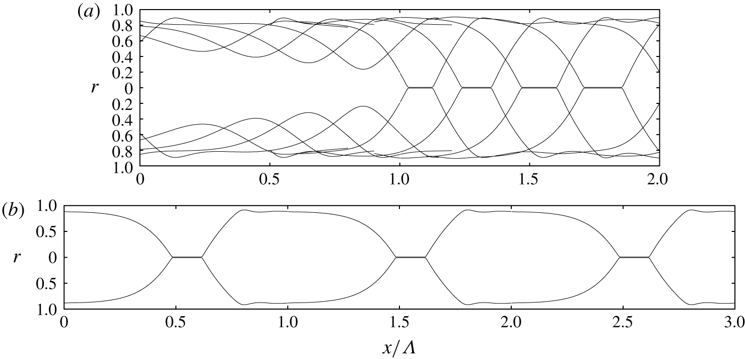
In our transient computations, the wavy liquid film can tend towards occluding the tube. In an experiment such an event would form a liquid plug separated by two gas bubbles. The topological change occurring in this situation cannot be mathematically represented by our model, which implies continuous fluid layers. Thus, we apply a numerical procedure to allow our computations to continue beyond such events. For this, we level the core radius  $d$ to an arbitrary value
 $d_{crit}=0.1$ whenever/wherever
 $d\leqslant d_{crit}$. As a result, occluded zones are represented by a thin gas filament connecting two bubbles either side of a liquid plug (figure 3c). Although our approach allows us to recover some basic features of these zones, it is a crude and invasive approximation of the actual physics. For example, every time
 $d$ is reset to
 $d_{crit}$, a bit of liquid mass is lost and this can cause the unphysical reopening of liquid plugs (supplementary movies M2 and M3, available at https://doi.org/10.1017/jfm.2020.267). We stress, however, that we are not interested in studying the actual behaviour of occluded zones here. Our current paper focuses on the events leading up to occlusion, and, thus, our numerical limitation of the core radius
 $d$ is simply a means to continue our computations until a developed state has been reached. Nonetheless, we propose in appendix E an alternative way of representing liquid plugs in the framework of our WRIBL model, based on an additional repulsive force in the momentum equation (2.5b) that stabilizes the film surface at very small
 $d$. This approach is inspired by the representation of contact line problems with film models (Thiele et al. Reference Thiele, Velarde, Neuffer and Pomeau2001), and confronting it with full-fledged plug models (Suresh & Grotberg Reference Suresh and Grotberg2005; Ubal et al. Reference Ubal, Campana, Giavedoni and Saita2008) is an enticing prospect for future work.
2.2 Direct numerical simulation
We have validated our model computations with selected DNS based on the full governing equations (2.1)–(2.4). These were performed with two different codes.
Transient simulations were performed with the finite volume solver Gerris (Popinet Reference Popinet2009), which uses the volume of a fluid (Hirt & Nichols Reference Hirt and Nichols1981) and continuum surface force (Brackbill, Kothe & Zemach Reference Brackbill, Kothe and Zemach1992) methods to represent the two-phase nature of the flow. We have successfully applied this code to falling liquid films in previous works (Dietze & Ruyer-Quil Reference Dietze and Ruyer-Quil2013, Reference Dietze and Ruyer-Quil2015; Dietze Reference Dietze2019), where further details are given. In the current work, we have used it to perform axisymmetric transient DNS on a domain spanning the wavelength  $\unicode[STIX]{x1D6EC}$ in streamwise direction and the tube radius
 $R$ in radial direction, applying periodic streamwise boundary conditions. To allow imposing the gas pressure drop
 $\unicode[STIX]{x0394}p_{g}$ (2.8) in this periodic setting, the streamwise momentum equations (2.1) for the liquid (
 $k=l$) and gas (
 $k=g$) were rewritten in terms of the modified pressure
 $\tilde{p}_{k}=p_{k}+x\unicode[STIX]{x0394}p_{k}/\unicode[STIX]{x1D6EC}$, yielding the additional source term
 $\unicode[STIX]{x1D6E4}_{k}$:
 $$\begin{eqnarray}\unicode[STIX]{x1D6E4}_{k}=\frac{\unicode[STIX]{x0394}p_{k}}{\unicode[STIX]{x1D6EC}},\quad \unicode[STIX]{x0394}p_{l}=\unicode[STIX]{x1D6F1}_{\unicode[STIX]{x1D70C}}\unicode[STIX]{x0394}p_{g}.\end{eqnarray}$$
Thanks to this source term, the governing equations can be solved with a periodicity condition on  $\tilde{p}_{k}$, while the actual pressure
 $p_{k}$ is subject to a pressure drop, allowing us to control the gas flow rate. Our transient DNS were started from a flat-film initial condition corresponding to the primary flow. All transient DNS were performed for case 4 in table 1, on a grid of square cells with increments
 $\unicode[STIX]{x1D6E5}_{x}=\unicode[STIX]{x1D6E5}_{r}=2^{-7}$ in the bulk of the fluid phases and
 $\unicode[STIX]{x1D6E5}_{x}=\unicode[STIX]{x1D6E5}_{r}=2^{-8}$ around the liquid–gas interface. The time step
 $\unicode[STIX]{x1D6E5}_{t}$ was dynamically adapted so that
 $w^{\star }\,\unicode[STIX]{x1D6E5}_{t}/\unicode[STIX]{x1D6E5}_{x}\leqslant 0.8$ in each cell, whereby
 $w^{\star }$ denotes the magnitude of the local dimensional velocity. We have verified that our simulations are grid independent. Results of our transient DNS are presented in appendix A, where they are used to validate our model computations.
The second DNS code allows us to construct travelling-wave solutions of (2.1)–(2.4) based on a pseudo-spectral approach, which we have integrated into the continuation software AUTO07P (Doedel Reference Doedel2008). This has allowed us to verify our numerical continuation results obtained with the WRIBL model (see figure 5d). In these travelling-wave DNS, the gas phase is not accounted for, i.e.  $\unicode[STIX]{x1D6F1}_{\unicode[STIX]{x1D707}}=\unicode[STIX]{x1D6F1}_{\unicode[STIX]{x1D70C}}=0$, and, thus, we have only applied them to case 3, where the effect of the gas is negligible. The underlying numerical procedure is detailed in appendix B.
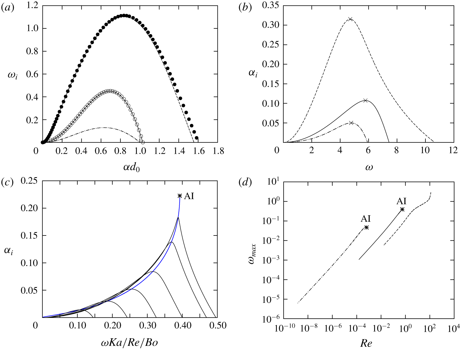
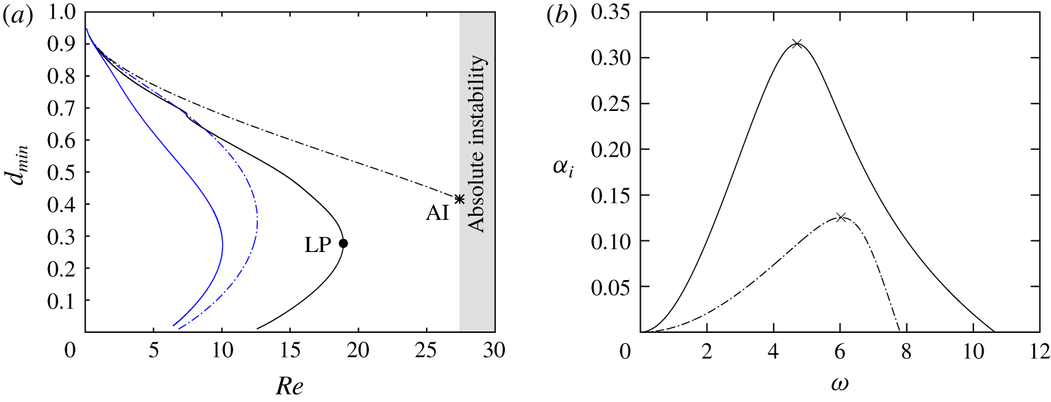
Linear instability predictions for three cases from table 1: case 1 (dot–dashed lines, diamonds); case 3 (solid lines, open circles); case 4 (dashed lines, filled circles). The core fluid is subject to an aerostatic pressure gradient  $\unicode[STIX]{x1D6F9}=1$. Lines correspond to the model dispersion relation (2.11). (a) Temporal growth:
 $\unicode[STIX]{x1D6FC}\in \mathbb{R}$,
 $\unicode[STIX]{x1D714}=\unicode[STIX]{x1D714}_{r}+\text{i}\unicode[STIX]{x1D714}_{i}$ in (2.10). Symbols correspond to the Orr–Sommerfeld solution, following the work of Hickox (Reference Hickox1971). (b) Spatial growth:
 $\unicode[STIX]{x1D714}\in \mathbb{R}$,
 $\unicode[STIX]{x1D6FC}=\unicode[STIX]{x1D6FC}_{r}+\text{i}\unicode[STIX]{x1D6FC}_{i}$ in (2.10). Crosses highlight maximal spatial growth. (c) Dispersion curves under increasing
 $Re\in [0.1,0.54]$. Blue line traces maximum growth rate
 $\unicode[STIX]{x1D6FC}_{i}(\unicode[STIX]{x1D714}_{max})$. (d) Most amplified angular velocity
 $\unicode[STIX]{x1D714}_{max}$ versus
 $Re$. Asterisks mark the absolute linear instability (AI) threshold.

2.3 Linear stability analysis
Linearizing the WRIBL model (2.5) around the uniform base state  $\{d,q_{k}\}=\{d_{0},q_{k0}\}$ and assuming a small-amplitude perturbation
 $\{d^{\prime },q_{k}^{\prime }\}$,
 $$\begin{eqnarray}\left.\begin{array}{@{}c@{}}d(x,t)=d_{0}+d^{\prime }(x,t)=d_{0}+\hat{d}\exp [\text{i}(\unicode[STIX]{x1D6FC}x-\unicode[STIX]{x1D714}t)]\\ q_{k}(x,t)=q_{k0}+q_{k}^{\prime }(x,t)=q_{k0}+\hat{q}_{k}\exp [\text{i}(\unicode[STIX]{x1D6FC}x-\unicode[STIX]{x1D714}t)]\end{array}\right\}\end{eqnarray}$$
yields the complex dispersion relation
 $$\begin{eqnarray}\displaystyle DR(\unicode[STIX]{x1D714},\unicode[STIX]{x1D6FC}) & = & \displaystyle 2\unicode[STIX]{x03C0}d_{0}\unicode[STIX]{x1D714}\{\unicode[STIX]{x1D700}_{jl}C_{jl}+\unicode[STIX]{x1D700}_{jg}\unicode[STIX]{x1D6F1}_{\unicode[STIX]{x1D707}}C_{jg}\}+\unicode[STIX]{x1D6FC}\{\unicode[STIX]{x2202}_{d}C_{jl}q_{j0}-\unicode[STIX]{x1D6F1}_{\unicode[STIX]{x1D707}}\unicode[STIX]{x2202}_{d}C_{jg}q_{j0}\}\nonumber\\ \displaystyle & & \displaystyle -\,2\unicode[STIX]{x03C0}d_{0}\unicode[STIX]{x1D6FC}^{2}M_{j}\unicode[STIX]{x1D700}_{jl}-\unicode[STIX]{x1D6FC}^{3}L_{j}q_{j0}-\text{i}ReWe\{\unicode[STIX]{x1D6FC}^{2}/d_{0}^{2}-\unicode[STIX]{x1D6FC}^{4}\}\nonumber\\ \displaystyle & & \displaystyle +\,\text{i}Re\{2\unicode[STIX]{x03C0}d_{0}[\unicode[STIX]{x1D714}^{2}(S_{g}-Sl)+\unicode[STIX]{x1D714}\unicode[STIX]{x1D6FC}(F_{jl}q_{j0}-F_{jg}q_{j0})]-\unicode[STIX]{x1D6FC}^{2}G_{jk}\},\end{eqnarray}$$
where  $j$ and
 $k$ are to be permuted over the phase indicators
 $l$ and
 $g$,
 $\unicode[STIX]{x1D714}$ designates the (complex) wave frequency,
 $\unicode[STIX]{x1D6FC}$ the (complex) wave number,
 $\unicode[STIX]{x1D700}_{ll}=\unicode[STIX]{x1D700}_{gg}=-1$, and
 $\unicode[STIX]{x1D700}_{lg}=\unicode[STIX]{x1D700}_{gl}=1$.
A temporal stability analysis assumes that waves grow self-similarly in their reference frame. This description implies  $\unicode[STIX]{x1D6FC}\in \mathbb{R}$ and
 $\unicode[STIX]{x1D714}=\unicode[STIX]{x1D714}_{r}+\text{i}\unicode[STIX]{x1D714}_{i}$, where the temporal growth rate
 $\unicode[STIX]{x1D714}_{i}$ is obtained by solving
 $DR(\unicode[STIX]{x1D714},\unicode[STIX]{x1D6FC})=0$. In figure 2(a) we have plotted the thus obtained dispersion curve
 $\unicode[STIX]{x1D714}_{i}(\unicode[STIX]{x1D6FC})$ of the temporal growth rate for cases 1, 3 and 4 from table 1. Lines correspond to the model dispersion relation (2.11), and symbols correspond to our own numerical solutions of the Orr–Sommerfeld equations, following the work of Hickox (Reference Hickox1971). Agreement between the two data sets is good. Thus, our model is able to accurately represent the linear wave selection.
In a spatially evolving film, it is more representative to consider the spatial growth rate  $\unicode[STIX]{x1D6FC}_{i}$. We thus solve
 $DR(\unicode[STIX]{x1D714},\unicode[STIX]{x1D6FC})=0$ for
 $\unicode[STIX]{x1D6FC}_{i}(\unicode[STIX]{x1D714})$, by assuming that
 $\unicode[STIX]{x1D714}\in \mathbb{R}$ and
 $\unicode[STIX]{x1D6FC}=\unicode[STIX]{x1D6FC}_{r}+\text{i}\unicode[STIX]{x1D6FC}_{i}$. In figure 2(b) we have plotted the thus obtained growth rate dispersion curves
 $\unicode[STIX]{x1D6FC}_{i}(\unicode[STIX]{x1D714})$ for the three cases from figure 2(a). Crosses mark the point of maximal growth rate and we denote
 $\unicode[STIX]{x1D714}_{max}$ the associated most amplified angular velocity.
In § 3.2 we will characterize occlusion by determining the limit of travelling-wave solutions through numerical continuation. This limit is very sensitive to the wave frequency  $f$. Thus, we focus on the spatially most amplified waves, which are most likely to emerge from linear wave selection in an experiment. For this, we impose the linearly most amplified frequency
 $f_{max}=2\unicode[STIX]{x03C0}/\unicode[STIX]{x1D714}_{max}$ in our continuation runs.
To determine  $f_{max}$, which changes with the control parameters varied in these runs, our continuation code was augmented to additionally solve for
 $\unicode[STIX]{x1D714}_{max}$ subject to
 $$\begin{eqnarray}DR(\unicode[STIX]{x1D714}_{max},\unicode[STIX]{x1D6FC})=0,\quad \unicode[STIX]{x2202}_{\unicode[STIX]{x1D714}}\unicode[STIX]{x1D6FC}_{i}|_{\unicode[STIX]{x1D714}=\unicode[STIX]{x1D714}_{max}}=0,\end{eqnarray}$$
where  $\unicode[STIX]{x2202}_{\unicode[STIX]{x1D714}}\unicode[STIX]{x1D6FC}_{i}$ is obtained from
 $\unicode[STIX]{x2202}_{\unicode[STIX]{x1D714}}DR=0$. In a given continuation run, the linear stability problem (2.12) is solved for the primary flow
 $\{q_{l0},q_{g0}\}=\{\bar{q}_{l},\bar{q}_{g}\}$, which is fixed by the mean flow rates
 $\bar{q}_{l}$ and
 $\bar{q}_{g}$ of the current travelling-wave solution.
As shown by Camassa et al. (Reference Camassa, Ogrosky and Olander2014), the annular falling liquid film can be subject to absolute instability. Thus, we have checked for the absolute instability (AI) threshold in all our continuation runs. In the context of our spatial stability analysis, where  $\unicode[STIX]{x1D714}\in \mathbb{R}$, the AI threshold bounds the solutions of (2.12) in terms of the varied control parameter, e.g.
 $Re$, because the maximum growth rate
 $\unicode[STIX]{x1D6FC}_{i}(\unicode[STIX]{x1D714}_{max})$ diverges there. For example, figure 2(c) represents the dispersion curves
 $\unicode[STIX]{x1D6FC}_{i}(\unicode[STIX]{x1D714})$ for case 3 at different values of
 $Re$, increased towards the AI threshold. The latter is marked by an asterisk on the blue curve, which traces the locus of the spatial growth rate maximum
 $\unicode[STIX]{x1D6FC}_{i}(\unicode[STIX]{x1D714}_{max})$. We point out that
 $\unicode[STIX]{x1D714}$ has been rescaled in figure 2(c).
Figure 2(d) represents how  $\unicode[STIX]{x1D714}_{max}$ changes with
 $Re$ for the three cases from figure 2(b). These curves allow us to discern the AI threshold (marked by asterisks) in terms of
 $Re$. For case 4 (dashed curve), we have truncated our solution at
 $Re=100$, beyond which our nonlinear model predictions are no longer reliable. The AI threshold lies beyond this point but, as we will see, the occlusion bound
 $Re_{max}$ lies well within the represented range (figure 6a).
In our current study, we focus on regimes where  $Bo\geqslant 1$. In this case, the AI threshold is always situated beyond the limit of nonlinear travelling-wave solutions and, thus, it does not affect the occlusion bound. However, we will demonstrate that neglecting certain physical effects in the mathematical description, such as axial viscous diffusion (figure 9b) or inertia (figure 12a), can change this.
3 Results and discussion
In §§ 3.1 and 3.2 we reproduce numerically the visualization experiments of Camassa et al. (Reference Camassa, Ogrosky and Olander2014) and demonstrate that the occlusion of a narrow tube by a wavy falling liquid film is caused by surface waves that do not possess a finite-amplitude travelling state. Depending on how these waves emerge in a spatially evolving film, either directly from linear instability (scenario I), or subsequent nonlinear dynamics (scenario II), different occlusion scenarios are possible. In § 3.2 we determine the bounds of these two scenarios based on the numerical continuation of travelling-wave solutions with our model (2.5). We obtain an upper conservative bound  $Re_{max}$, above which occlusion in a naturally evolving film is certain, and a lower conservative bound
 $Re_{0}$, below which occlusion is impossible. These bounds delimit a regime of conditional occlusion,
 $Re_{0}<Re<Re_{max}$, where occlusion is theoretically possible but does not necessarily occur in a real system.
In § 3.7 we demonstrate occlusion scenarios I and II, which are associated with the regimes of certain ( $Re>Re_{max}$) and conditional occlusion (
 $Re_{0}<Re<Re_{max}$), by reproducing two of the experiments in Dao & Balakotaiah (Reference Dao and Balakotaiah2000) with our own spatio-temporal computations. Before that, in §§ 3.3 to 3.6, we establish how different physical effects, i.e. gravity, axial viscous diffusion, inertia and the core gas flow, affect the upper conservative bound
 $Re_{max}$, which delimits these two regimes. Except for § 3.6, where we will vary the gas Reynolds number
 $Re_{g}$, our computations have been performed for an aerostatic pressure drop, i.e.
 $\unicode[STIX]{x1D6F9}=1$. This is most representative of experiments in a quiescent gas.
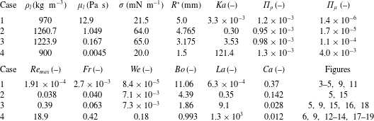
Representative parameters for our computations. Liquid properties correspond to a high-viscosity silicone oil (case 1), glycerol–water mixtures concentrated at 99 % and 89 % by mass (cases 2 and 3), and a low-viscosity silicone oil (case 4), while the core fluid is air with  $\unicode[STIX]{x1D707}_{g}=1.8\times 10^{-5}~\text{Pa}~\text{s}$ and
 $\unicode[STIX]{x1D70C}_{g}=1.2~\text{kg}~\text{m}^{-3}$. Case 1 corresponds to figure 3(a) in Camassa et al. (Reference Camassa, Ogrosky and Olander2014), and cases 2 and 3 correspond to experimental runs 20 and 13 in Dao & Balakotaiah (Reference Dao and Balakotaiah2000). The dimensionless groups are
 $Bo=\unicode[STIX]{x1D70C}_{l}g{\mathcal{L}}^{2}/\unicode[STIX]{x1D70E}$,
 $Ca=\unicode[STIX]{x1D707}_{l}{\mathcal{U}}/\unicode[STIX]{x1D70E}$,
 $Re=\unicode[STIX]{x1D70C}_{l}{\mathcal{U}}{\mathcal{L}}/\unicode[STIX]{x1D707}_{l}$,
 $Ka=\unicode[STIX]{x1D70E}\unicode[STIX]{x1D70C}_{l}^{-1}g^{-1/3}\unicode[STIX]{x1D707}_{l}^{-4/3}$,
 $La=\unicode[STIX]{x1D70E}\unicode[STIX]{x1D70C}_{l}{\mathcal{L}}/\unicode[STIX]{x1D707}_{l}^{2}$,
 $We=\unicode[STIX]{x1D70C}_{l}{\mathcal{U}}^{2}{\mathcal{L}}/\unicode[STIX]{x1D70E}$ and
 $Fr={\mathcal{U}}/\sqrt{g{\mathcal{L}}}$, where
 ${\mathcal{L}}=R^{\star }$ and
 ${\mathcal{U}}=q_{l0}^{\star }/\unicode[STIX]{x03C0}/{\mathcal{L}}^{2}$,
 $q_{l0}^{\star }$ designating the dimensional nominal liquid flow rate. We denote by
 $Re_{max}$ the upper conservative occlusion bound (see e.g. figures 5a and 5b).

Parameters for our computations are varied around the four cases listed in table 1, which represent real liquids and plausible values of the tube radius. Case 1 corresponds to figure 3(a) in Camassa et al. (Reference Camassa, Ogrosky and Olander2014), where the working liquid was a high-viscosity silicone oil. Cases 2 and 3 correspond to experimental runs 20 and 13 in Dao & Balakotaiah (Reference Dao and Balakotaiah2000), where glycerol–water mixtures concentrated at 99 % and 89 % by mass were used. Finally, case 4 concerns a liquid film of low-viscosity silicone oil. The four cases cover a considerable range of the Laplace number  $La=\unicode[STIX]{x1D70E}\unicode[STIX]{x1D70C}_{l}R^{\star }/\unicode[STIX]{x1D707}_{l}^{2}$, which relates capillarity to viscous drag, and the Reynolds number, which we have quantified with
 $Re_{max}$. We see that inertia, which drives the Kapitza instability, is significant for case 4. For this case, which is the most challenging, we have validated our model computations with transient DNS in appendix A (comparisons with travelling-wave DNS, for case 3, are reported in figure 5d).
3.1 Nature of the surface waves that cause occlusion
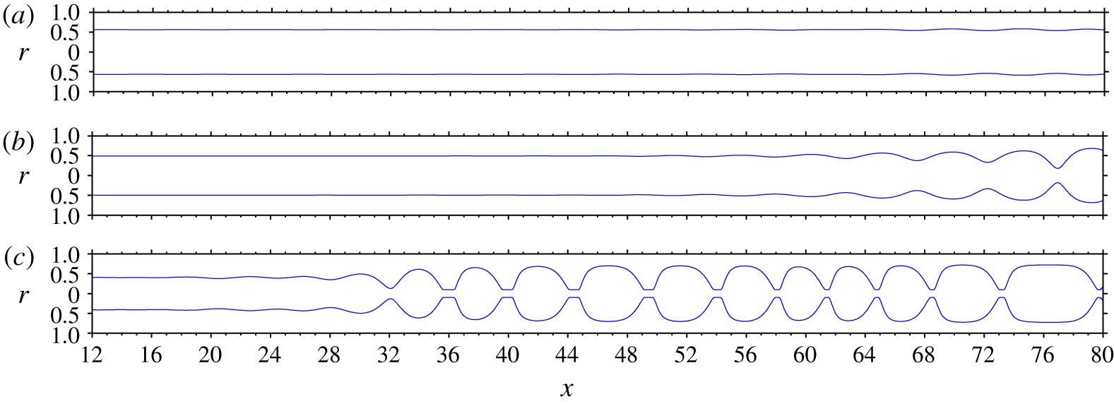
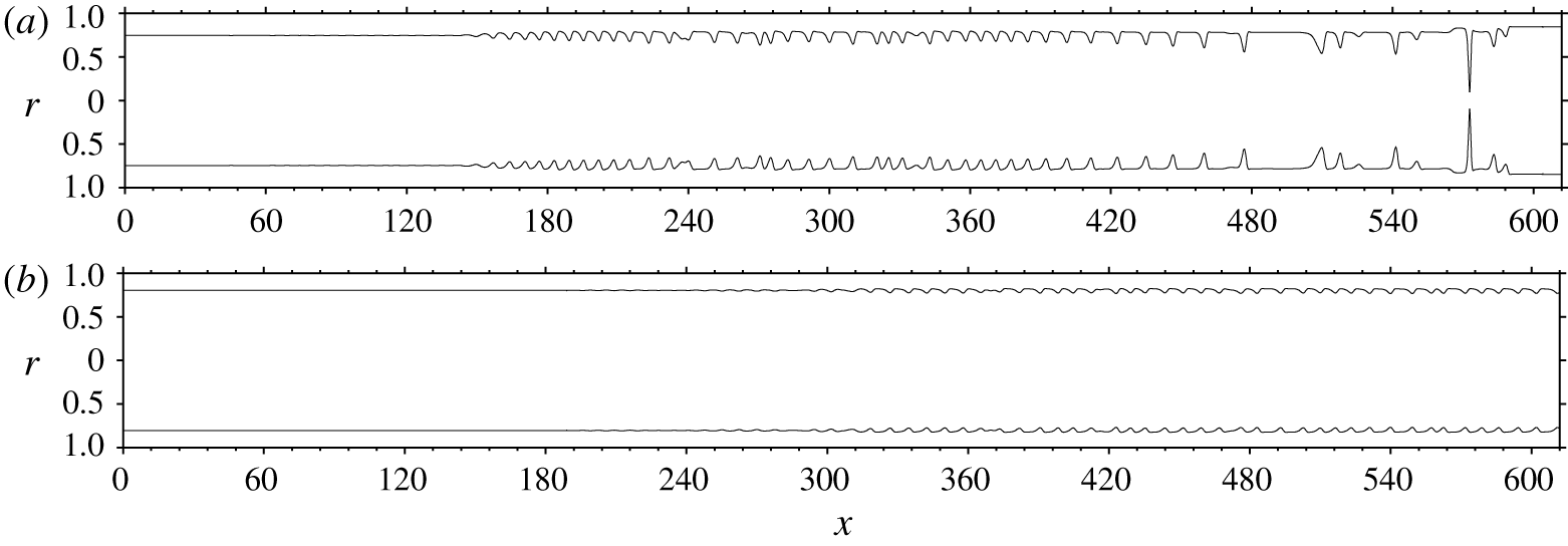
Spatio-temporal computations of the experiments in figures 3(a), 3(b) and 3(c) of Camassa et al. (Reference Camassa, Ogrosky and Olander2014), which were performed in an  $L^{\star }=400~\text{mm}$ tube. Parameters correspond to case 1 in table 1. Computations were performed with our model (2.5) using inlet/outlet conditions and the noisy inlet perturbation (2.6), where we set
 $\unicode[STIX]{x1D716}_{1}=0$ and adjusted
 $\unicode[STIX]{x1D716}_{2}$ to match the experimental wave growth. (a)
 $Re=2.3\times 10^{-4}$,
 $q_{l0}^{\star }=4.8\times 10^{-2}~\text{cm}^{3}~\text{s}^{-1}$,
 $\unicode[STIX]{x1D716}_{2}=0.0002$; (b)
 $Re=3.2\times 10^{-4}$,
 $q_{l0}^{\star }=6.7\times 10^{-2}~\text{cm}^{3}~\text{s}^{-1}$,
 $\unicode[STIX]{x1D716}_{2}=0.00005$; (c)
 $Re=4.5\times 10^{-4}$,
 $q_{l0}^{\star }=9.4\times 10^{-2}~\text{cm}^{3}~\text{s}^{-1}$,
 $\unicode[STIX]{x1D716}_{2}=0.0001$.

Camassa et al. (Reference Camassa, Ogrosky and Olander2014) performed occlusion experiments in an  $R^{\star }=0.5~\text{mm}$ and
 $L^{\star }=400~\text{mm}$ transparent tube using high-viscosity silicone oil (case 1 in table 1). In their figure 3, the authors produce photographs of the wavy falling liquid film at different
 $Re$ beyond the experimental occlusion threshold, allowing us to discern the nature of the surface waves that cause occlusion. We have reproduced three of these experiments with spatio-temporal computations based on our model (2.5) on a long domain using inlet/outlet conditions (see § 2.1). Experimental noise was mimicked through the noisy inlet perturbation (2.6), where we set
 $\unicode[STIX]{x1D716}_{1}=0$, and tuned
 $\unicode[STIX]{x1D716}_{2}$ to match the spatial evolution of surface waves in the experiments (when decreasing/increasing
 $\unicode[STIX]{x1D716}_{2}$, the region of linear growth of surface waves is stretched/compressed in streamwise direction and this shifts the emergence of nonlinear effects, such as occlusion, downstream/upstream). In figure 3 we show snapshots of these computations, which are to be directly compared to figures 3(a), 3(b) and 3(c) in Camassa et al. (Reference Camassa, Ogrosky and Olander2014).
Agreement with the experimental snapshots is good. In particular, the wavelength of the four distinct surface waves at the tube outlet in figure 3(b) is predicted accurately by our computations. Also, the number of gas bubbles (eleven) in figure 3(c), which result from successive occlusion events, agrees with the experiment. Figure 3(c) and the supplementary movie M1 allow us to discern the actual mechanics of occlusion. Surface waves in the upstream portion of the tube grow spatially until their crests reach the tube axis, whereupon individual bubbles of the gas core are pinched off. Our model accurately predicts the length scale of the pinch-off process in comparison with the experiment. We stress that figure 3(c) is a snapshot and that the occlusion point shifts up and down the tube intermittently as a result of the noisy wave spectrum imposed through the inlet condition. These results show that our model captures accurately the wave dynamics leading up to occlusion, and this is the focus of our current study. However, the physics of the liquid plugs resulting from occlusion is captured only very crudely by the numerical core radius limitation introduced in § 2.1. For example, the shape of the gas bubbles in figure 3(c) is quite different from that in the experiment and their length evolves as they travel downstream (see also supplementary movie M1). First results reported in appendix E suggest that these shortcomings can be alleviated with our improved WRIBL model. But the exact shape of liquid plugs can never be fully captured in the context of lubrication theory, as the film surface slope diverges at their edges.
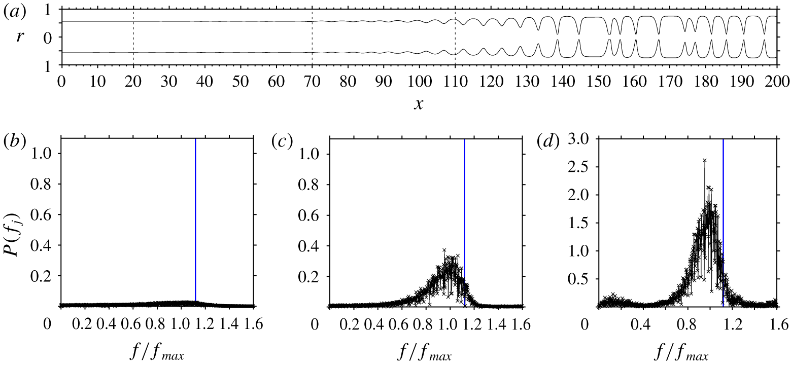
Nature of the prevailing surface waves that cause occlusion. Spatio-temporal computation reproducing the second version of the experiment in figure 3(a) of Camassa et al. (Reference Camassa, Ogrosky and Olander2014), which was performed in a longer  $L^{\star }=1~\text{m}$ tube: case 1 in table 1,
 $Re=2.3\times 10^{-4}$. (a) Snapshot of the computed film profile, showing individual surface waves that cause occlusion in the region
 $x\geqslant 130$. (b–d) Frequency spectra at different streamwise locations leading up to the occlusion region (marked by dashed lines in panel a): (b)
 $x=20$; (c)
 $x=70$; (d)
 $x=110$. Vertical blue lines at
 $f/f_{max}=1.12$ mark the limit of travelling-wave solutions determined by numerical continuation (see figure 6b). Here
 $f_{max}$ designates the spatially most amplified frequency of linear waves.

We now focus on figure 3(a), where  $Re$ is closest to the experimental occlusion threshold. For this case, Camassa et al. (Reference Camassa, Ogrosky and Olander2014) observed occlusion only after having switched to a longer
 $L^{\star }=1~\text{m}$ tube. Because of the small spatial growth rate, distinguishable surface waves emerged only very close to the outlet of the shorter
 $L^{\star }=400~\text{mm}$ tube, and their amplitude was insufficient to cause occlusion there. Our computation in figure 3(a) exhibits the same behaviour.
We have also reproduced numerically the experiment in the  $L^{\star }=1~\text{m}$ tube and a snapshot of our computation is represented in figure 4(a). It confirms that occlusion does indeed occur, in the region
 $x\geqslant 130$. Occlusion results from unbounded spatial growth of the prevailing surface waves, and figures 4(b) to 4(d) show how the latter emerge from the noisy inlet condition. In these panels, we have represented the single-sided amplitude spectrum
 $P(f_{j})$ of the discrete Fourier transform
 $F(f_{j})$ applied to core radius time series
 $d(t_{k})$ recorded at different streamwise positions
 $x$ (marked by dashed lines in figure 4a), leading up to the occlusion region
 $$\begin{eqnarray}P(f_{j})=(2/N)F(f_{j})\;\forall \;j\leqslant N/2+1,\quad F(f_{j})=\mathop{\sum }_{k=0}^{N}d(t_{k})\exp (\text{i}2\unicode[STIX]{x03C0}j/Nk),\end{eqnarray}$$
where  $N=1.8\times 10^{6}$ is the number of (equidistant) sampling points
 $t_{k}$ with which we have recorded the time series
 $d(t_{k})$ over a duration
 $T=9.1\times 10^{4}$, and
 $f_{j}=(j/N)/T$ are the frequencies of the discrete spectrum. At the most downstream location (figure 4d), the spectrum is organized around the spatially most amplified frequency of linear waves
 $f_{max}$ in the form of a quite narrow peak. This peak lies beyond the limit
 $f/f_{max}=1.12$ for the existence of travelling-wave solutions at the considered Reynolds number
 $Re=2.3\times 10^{-4}$, which is highlighted by vertical blue lines in figures 4(b), 4(c) and 4(d). This limit has been determined by numerical continuation of travelling-wave solutions, which we will discuss in the next subsection (it is marked by an asterisk in figure 5b). We will see that higher frequency (shorter) waves are safe from and lower frequency (longer) waves are prone to occlusion.
By way of numerical continuation, Camassa et al. (Reference Camassa, Ogrosky and Olander2014) were the first to show that the existence of travelling-wave solutions is bounded. By increasing  $Re$ at fixed wavelength, the authors found a limit point beyond which travelling-wave solutions cease to exist. They conjectured that the loss of such solutions signals occlusion in an actual experiment. However, the authors cautioned that further work was needed to verify this conjecture. This work was initiated by Camassa et al. (Reference Camassa, Marzuola, Ogrosky and Vaughn2016), but their model did not account for axial viscous diffusion. Our computations in figures 3 and 4 provide further validation, by taking into account this effect, which greatly improves agreement of our model predictions with the experiments of Camassa et al. (Reference Camassa, Ogrosky and Olander2014), as a result of the high viscosity of the working liquid. For example, when running the computation in figure 4(a) without axial viscous diffusion, we did not observe any occlusion over the entire experimental tube length (see figure 21 in appendix D), which is in qualitative contradiction to the experiments. Also, we will show in § 3.4 that neglecting axial viscous diffusion increases
 $Re_{max}$ by 74 % for this liquid (figure 9a), moving it far beyond the experimental occlusion limit, as quantified in terms of
 $Re$.
Figure 4 proves that the occlusion of a narrow tube by a wavy falling liquid film is caused by surface waves that lie beyond the limit of travelling-wave solutions. Thus, occlusion can be characterized based on the existence span of such solutions and we proceed to this in the following subsection.
3.2 Travelling waves: regimes of certain, conditional and impossible occlusion
The frequency of travelling waves determines their amplitude, which is well known for planar falling liquid films (Nosoko et al. Reference Nosoko, Yoshimura, Nagata and Oyakawa1996) and also holds in our cylindrical configuration. At a given value of  $Re$, the smaller the wave frequency, the greater the wave amplitude. Consequently, low-frequency travelling waves are more prone to occlusion than high-frequency waves. This effect was demonstrated by Camassa et al. (Reference Camassa, Marzuola, Ogrosky and Vaughn2016) and Ding et al. (Reference Ding, Liu, Liu and Yang2019) with a first-order asymptotic model and a lubrication model, respectively. Using our model (2.5), we quantify it for the real liquids studied here (cases 1–4 in table 1), which require a more complicated modelling approach.
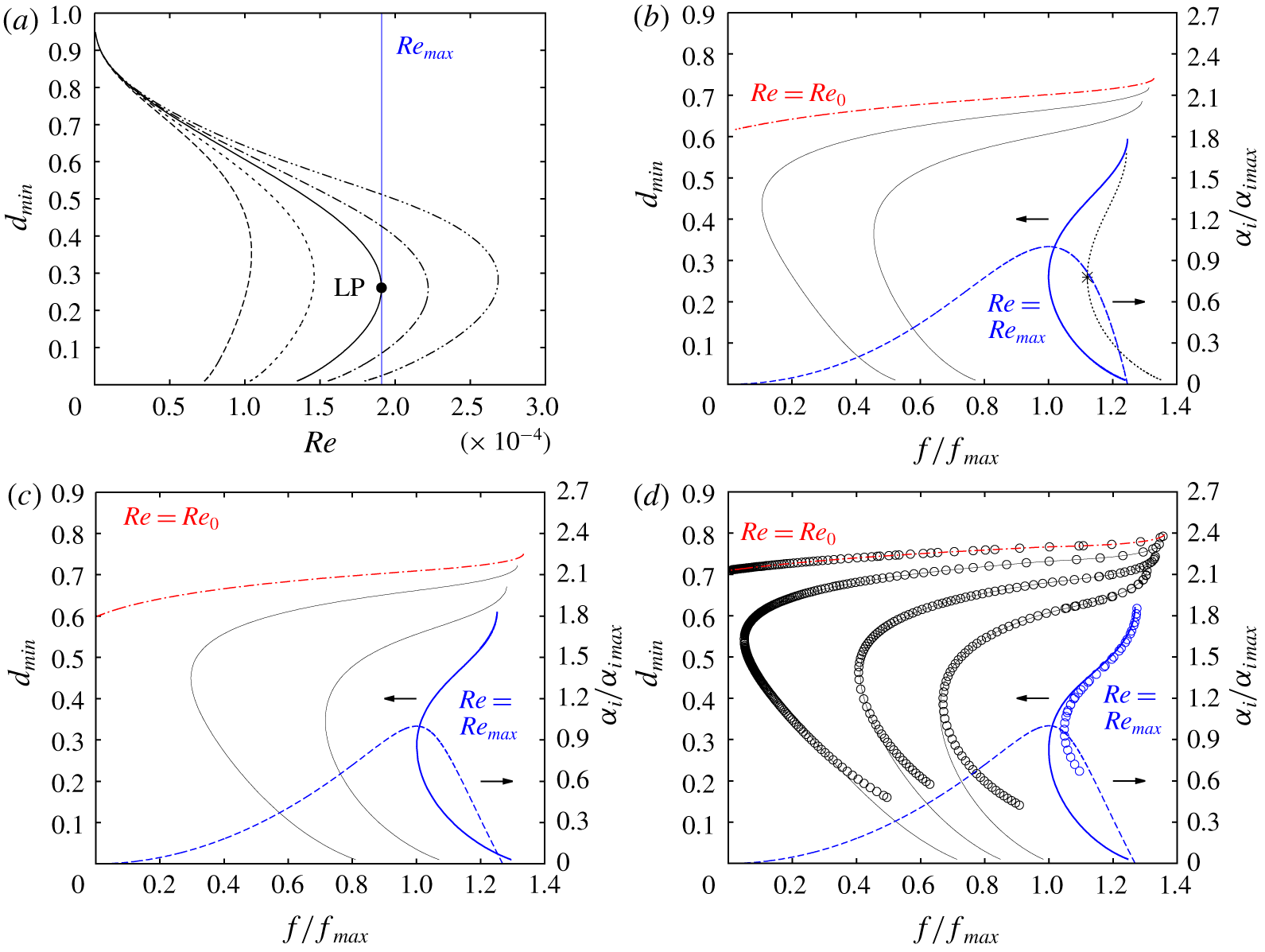
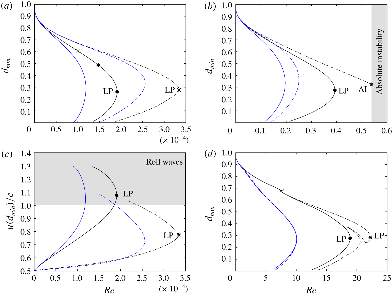
Figure 5(a) represents curves of travelling-wave solutions for case 1 in terms of the minimal core radius  $d_{min}$, as obtained by varying the liquid Reynolds number
 $Re$. On each curve, we have fixed the wave frequency
 $f$ to a certain fraction
 $f/f_{max}$ of the spatially most amplified frequency
 $f_{max}$, which we determine through the approach outlined in § 2.3. All curves display a limit point in terms of
 $Re$, beyond which there are no travelling-wave solutions. The existence of such a limit point was discovered by Camassa et al. (Reference Camassa, Ogrosky and Olander2014), who imposed a constant wavelength in their continuation. This wavelength was too long compared to their experiments, whereas we see here that accounting for the correct wavelength/frequency is quite important. Indeed, the limit point of the curves in figure 5(a) varies greatly with
 $f/f_{max}$. The lower the wave frequency, the smaller the limit value of
 $Re$, the more danger of occlusion.
Limits of travelling-wave solutions obtained from numerical continuation with our model (2.5). Cases 1 (panels a,b), 2 (panel c) and 3 (panel d) in table 1. (a) Continuation of  $Re$ at wave frequency
 $f/f_{max}=0.5$ (long dashes), 0.8 (short dashes), 1 (solid), 1.1 (dot–dashed), and 1.2 (dot–dot–dashed). The vertical blue line marks the limit point for spatially most amplified linear waves, where
 $f=f_{max}$ and
 $Re=Re_{max}$. (b–d) Frequency dependence at
 $Re=\text{const}$. Dashed blue: linear spatial growth rate
 $\unicode[STIX]{x1D6FC}_{i}$ at
 $Re=Re_{max}$ (right abscissae). Other: travelling-wave solutions at
 $Re=\text{const.}$ (left abscissae). (b) Case 1:
 $Re=Re_{0}=6\times 10^{-5}$ (dot–dashed red),
 $Re=7.5\times 10^{-5}$,
 $1\times 10^{-4}$ (thin solid),
 $Re=Re_{max}=1.91\times 10^{-4}$ (thick solid blue), and
 $Re=2.3\times 10^{-4}$ (dotted with asterisk). (c) Case 2:
 $Re=Re_{0}=0.012$ (dot–dashed red),
 $Re=0.016$, 0.025 (thin solid), and
 $Re=Re_{max}=0.038$ (thick solid). (d) Case 3:
 $Re=Re_{0}=0.075$ (dot–dashed red),
 $Re=0.1$, 0.14, 0.2 (thin solid), and
 $Re=Re_{max}=0.393$ (thick solid). Open circles correspond to data obtained with our own travelling-wave DNS (see § 2.2).

We now introduce the upper conservative occlusion bound  $Re_{max}$, which corresponds to the limit point (LP) of the solid line representing the spatially most amplified travelling waves, i.e.
 $f/f_{max}=1$. For
 $Re>Re_{max}$, the linearly most amplified surface waves, which are most likely to emerge in an experiment, do not possess travelling states and occlusion is certain to occur in a naturally evolving film. The experiment of Camassa et al. (Reference Camassa, Ogrosky and Olander2014), which we have reproduced numerically in figure 4, corresponds to this regime. Occlusion in this case occurs through scenario I, which we will discuss further in § 3.7 based on spatio-temporal computations.
Figure 5(b) explains the meaning of the upper occlusion bound  $Re_{max}$ in a different way, by illustrating the effect of the wave frequency
 $f$ at fixed
 $Re$. The dashed blue line represents the linear spatial growth rate
 $\unicode[STIX]{x1D6FC}_{i}$ at
 $Re=Re_{max}$ (right abscissa), while all other curves represent travelling-wave solutions (left abscissa) at different
 $Re$. These curves all display a limit point in terms of
 $f$. The dotted line marked by an asterisk corresponds to the experiment of Camassa et al. (Reference Camassa, Ogrosky and Olander2014) numerically reproduced in figure 4, where
 $Re=2.3\times 10^{-4}$. The thick blue solid line corresponds to the upper occlusion bound
 $Re=Re_{max}=1.9\times 10^{-4}$ and its limit point thus coincides with the maximum of the growth rate dispersion curve
 $\unicode[STIX]{x1D6FC}_{i}(f)$. We stress that determining
 $Re_{max}$ requires simultaneously computing the most amplified wave frequency
 $f_{max}$ in our numerical continuations, as described in § 2.3. This had not been attempted in the previous studies of Camassa et al. (Reference Camassa, Ogrosky and Olander2014) and Ding et al. (Reference Ding, Liu, Liu and Yang2019).
Reducing  $Re$ below
 $Re_{max}$ moves the limit point of travelling-wave solutions to lower values of
 $f$. Thus, the occlusion range is increasingly confined to (very long) waves of very low frequency, until it vanishes completely at
 $Re=Re_{0}$ (red dot–dashed curve in figure 5b). This limit, the existence of which was discovered by Ding et al. (Reference Ding, Liu, Liu and Yang2019), constitutes a lower conservative occlusion bound. When
 $Re<Re_{0}$, occlusion is impossible, no matter how long the waves. In a real system, it is conceivable that wave coalescence events can produce local overshoots leading to occlusion even when
 $Re<Re_{0}$. However, we have not observed this in our computations of spatially evolving films (see figures 16b and 17c). The value
 $Re_{0}$ being very low for all studied liquids, inertia is weak and significant overshoots are unlikely.
Based on the conservative occlusion bounds  $Re_{0}$ and
 $Re_{max}$, we delimit a region of conditional occlusion,
 $Re_{0}<Re<Re_{max}$ (between the red dot–dashed and thick solid blue lines in figure 5b), where occlusion is theoretically possible, for long enough waves, but does not necessarily occur in a real system. That depends on whether the required waves actually develop in a spatially evolving film. And, in particular, whether the tube is long enough to accommodate the nonlinear wave dynamics required to produce them. In § 3.7 we will demonstrate that occlusion in this regime occurs through scenario II, i.e. wave coarsening triggered by secondary instability, which shifts surface waves down the ascending branch of the dispersion curve towards increasingly low frequencies.
In figure 5(a), the limit point is a turning point, where two solution branches meet. As suggested by Camassa et al. (Reference Camassa, Ogrosky and Olander2014), we have checked their stability using transient periodic simulations with imposed  $\unicode[STIX]{x1D6F9}$ started from selected travelling-wave solutions. In these computations, numerical noise is responsible for perturbing the flow. A full-fledged formal stability analysis, such as the one performed by Camassa et al. (Reference Camassa, Marzuola, Ogrosky and Vaughn2016) based on the first-order model of Camassa et al. (Reference Camassa, Ogrosky and Olander2014), is outside the scope of our current study. We find that the lower solution branch is entirely unstable. As this branch does not connect to the flat-film primary flow
 $d_{min}=d_{max}=1$, the solutions thereon are thus highly unlikely in an experiment. Conversely, the upper branch is stable, at least with respect to periodic perturbations. However, wave trains of high-frequency travelling waves on falling liquid films are subject to secondary subharmonic and sideband instabilities that rely on wave interaction and lead to coalescence events (Liu & Gollub Reference Liu and Gollub1993). We have found that this triggers occlusion scenario II, which we will demonstrate in § 3.7. Finally, when starting a periodic transient computation from a flat-film initial condition beyond the limit of travelling-wave solutions, the outcome is indeed occlusion, which we have checked (and validated with transient DNS) in appendix A (see figures 19a and 19b).
Figures 5(c) (case 2), 5(d) (case 3) and 6 (case 4) report the occlusion bounds  $Re_{max}$ and
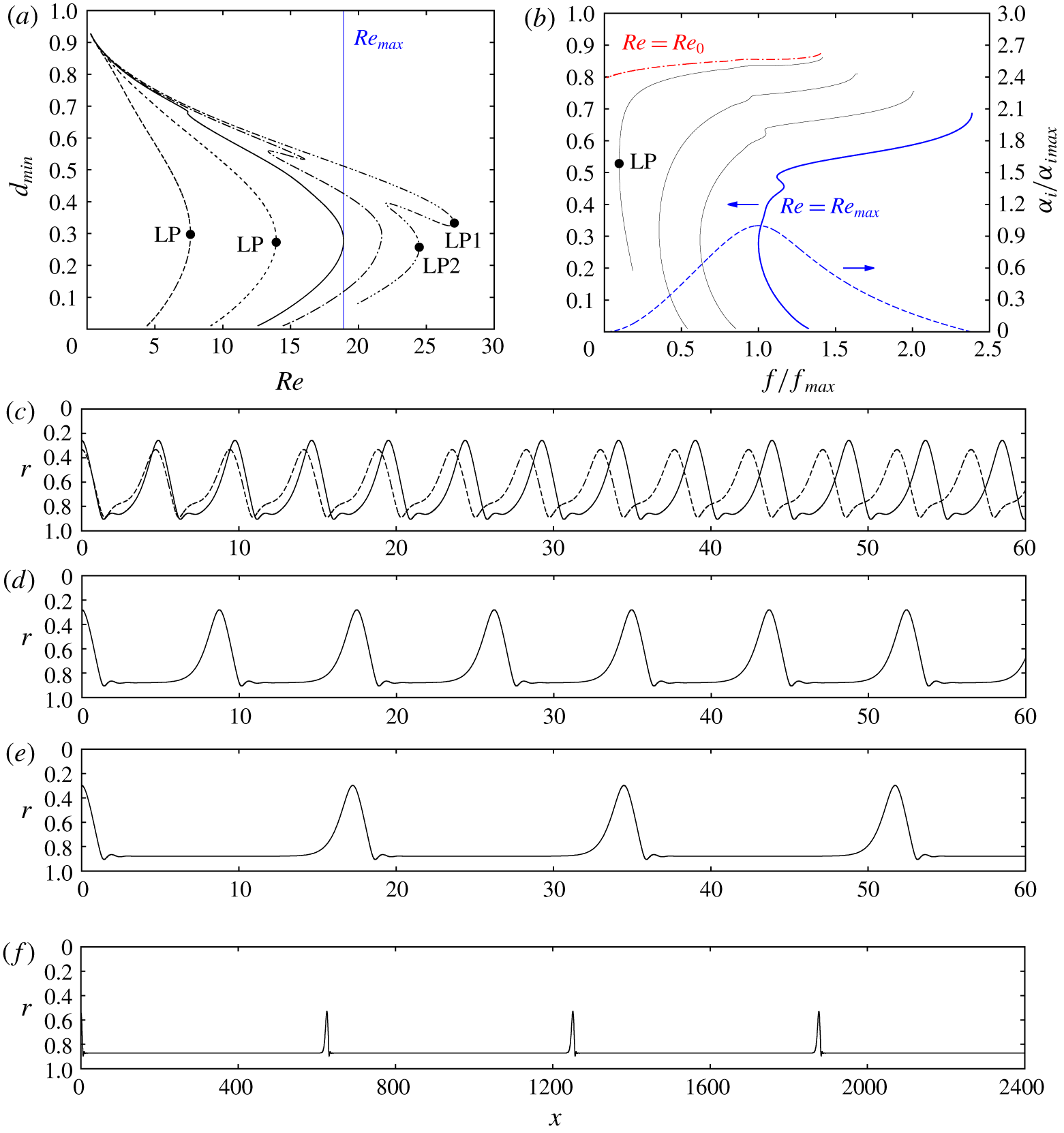
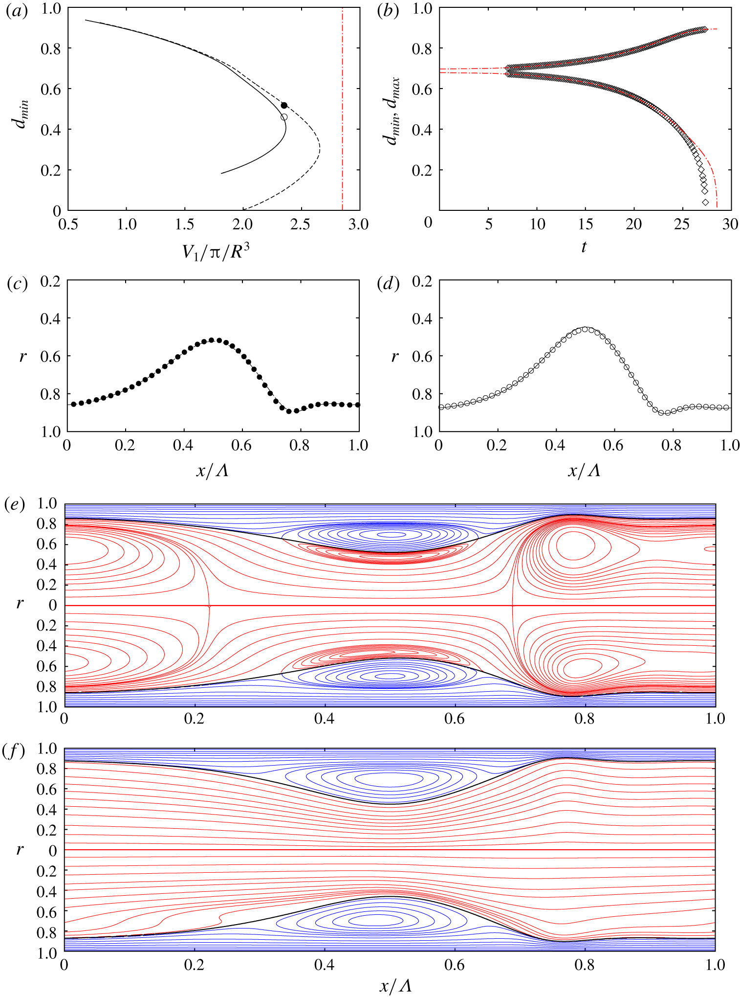
 $Re_{0}$ for the other three cases from table 1. In figure 5(d) we have represented with open circles additional results obtained with our own travelling-wave DNS (see § 2.2), evidencing gratifying agreement with our WRIBL model predictions. Overall tendencies in these graphs are the same as for case 1. For case 4 (low-viscosity silicone oil), where the Kapitza instability is relevant, there is an additional feature. In figure 6(a), the continuation curves of
 $d_{min}$ (
 $Re$,
 $f=\text{const.}$) at high frequencies, e.g. the dot–dot–dashed curve at
 $f/f_{max}=1.2$, exhibit two lobes that are each associated with a limit point. Wave profiles corresponding to these highlighted points LP1 and LP2 are represented in figure 6(c). We see that the main wave hump is preceded by a small precursory ripple. Such so-called capillary ripples can produce multiplicity of solutions in falling liquid films, when they are close enough to interact with the following wave hump (Kalliadasis et al. Reference Kalliadasis, Ruyer-Quil, Scheid and Velarde2012). By contrast, the dashed curves in figure 6(a), which pertain to low-frequency waves, each display only a single limit point. In figures 6(d) and 6(e) we show the corresponding wave profiles at those points. We see in figures 6(c), 6(d) and 6(e) that lower wave frequencies are associated with longer wavelengths, which we have implicitly assumed up until now.
Limits of travelling-wave solutions for case 4 in table 1. (a) Continuation of  $Re$ at constant wave frequency
 $f/f_{max}=0.5$ (long dashes), 0.8 (short dashes), 1 (solid), 1.1 (dot–dashed) and 1.2 (dot–dot–dashed). (b) Frequency dependence at
 $Re=\text{const}$. Dashed: linear spatial growth rate
 $\unicode[STIX]{x1D6FC}_{i}$ at
 $Re=Re_{max}=18.9$ (right abscissa). Other: travelling-wave solutions (left abscissa) at
 $Re=Re_{0}=1.5$ (dot–dashed red),
 $Re=2$, 5, 10 (thin solid), and
 $Re=Re_{max}$ (thick blue). (c–e) Film profiles for LPs marked by filled circles in panel a; (c)
 $f=1.2f_{max}$. Solid, LP1; dashed, LP2; (d)
 $f=0.8f_{max}$; (e)
 $f=0.5f_{max}$; (f) profile for marked LP in panel (b).

Finally, figure 6(f) represents the wave profile corresponding to the limit point marked by a filled circle on the  $Re=2$ curve in figure 6(b). This curve lies in the region of conditional occlusion,
 $Re_{0}<Re<Re_{max}$ (
 $Re_{0}=1.5$,
 $Re_{max}=18.9$). However, based on the wavelength of the waves in figure 6(f), which span about 600 times the tube radius, it becomes clear that quite particular conditions can be required to cause occlusion in this regime. This underlines the conservative nature of the lower occlusion bound
 $Re_{0}$.
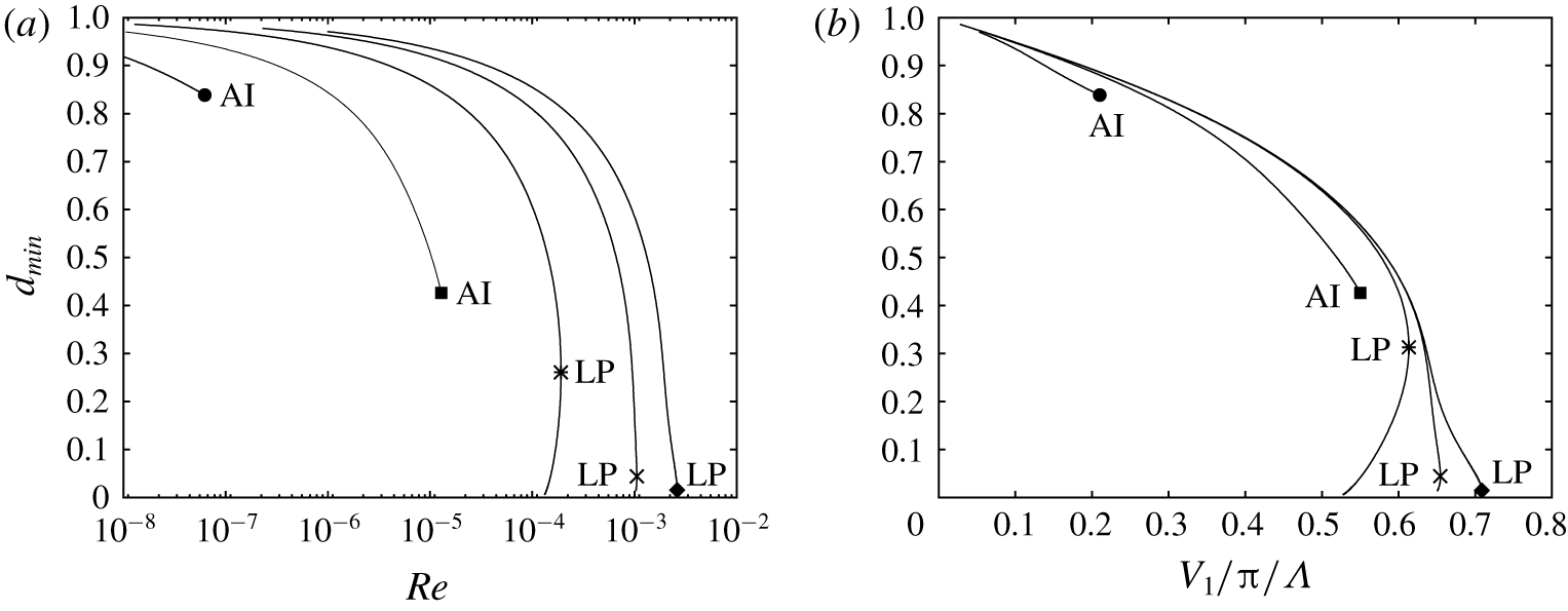
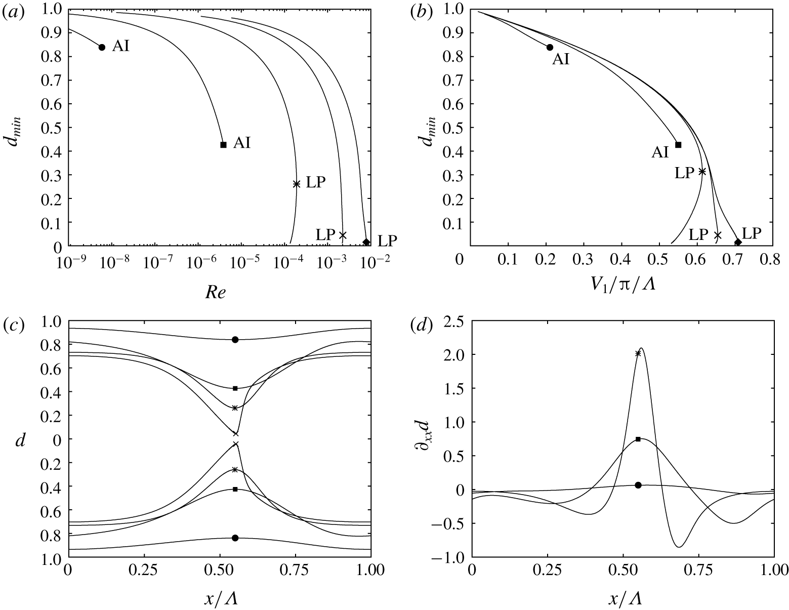
Delay of occlusion by increasing the Bond number  $Bo=\unicode[STIX]{x1D70C}_{l}gR^{\star 2}/\unicode[STIX]{x1D70E}$ at constant Laplace number:
 $La=\unicode[STIX]{x1D70E}\unicode[STIX]{x1D70C}_{l}R^{\star }/\unicode[STIX]{x1D707}_{l}^{2}=6.27\times 10^{-4}$ (case 1). Travelling-wave solutions at
 $f=f_{max}$. Symbols mark onset of absolute linear instability (AI) or limit points (LP). The limit points correspond to the upper occlusion bound
 $Re_{max}$. Circles,
 $Bo=0.1$; squares,
 $Bo=1$; asterisks,
 $Bo=11.1$ (case 1); crosses,
 $Bo=50$; diamonds,
 $Bo=100$. (a) Minimal core radius
 $d_{min}$ versus liquid Reynolds number. (b) Minimal core radius versus liquid holdup.

In summary, due to the frequency dependence of travelling-wave solutions demonstrated in figures 5(b), 5(c), 5(d) and 6(b), three characteristic regimes can be delimited: (i) impossible occlusion, when  $Re<Re_{0}$; (ii) conditional occlusion, when
 $Re_{0}<Re<Re_{max}$; and (iii) certain occlusion, when
 $Re>Re_{max}$. In § 3.7 we will characterize these regimes with spatio-temporal computations and demonstrate the associated occlusion scenarios I and II. On the other hand, the frequency dependence of travelling-wave solutions opens the possibility of using coherent inlet forcing to prevent occlusion. By forcing regular waves of sufficiently high frequency, occlusion can be avoided versus a noise-driven wave evolution. We demonstrate this idea in § 3.8 based on spatio-temporal computations. In the next sections, § 3.3 to § 3.6, we first proceed to establish how different physical effects, i.e. gravity, axial viscous diffusion, inertia and the core gas flow, affect the upper conservative occlusion bound
 $Re_{max}$.
3.3 Role of gravity
The upper occlusion bound  $Re_{max}$ can be significantly delayed by increasing the relative strength of gravity versus capillarity. We have quantified this by varying the Bond number
 $Bo=\unicode[STIX]{x1D70C}_{l}gR^{\star 2}/\unicode[STIX]{x1D70E}$ over several orders of magnitude at constant Laplace number
 $La=6.3\times 10^{-4}$. This value of
 $La$ corresponds to the high-viscosity silicone oil (case 1), where inertia is always negligible.
Figure 7(a) represents travelling-wave solutions for different values of  $Bo$. On each curve we have imposed the frequency
 $f_{max}$ of the most amplified spatially growing linear waves. All curves exhibit a limit value for the liquid Reynolds number
 $Re$. For
 $Bo\ll 1$, where the Plateau–Rayleigh instability dominates, this limit is dictated by the onset of absolute instability, as discussed in figures 2(c) and 2(d). Beyond this point, prevailing waves are no longer characterized by the most amplified spatially growing linear waves and
 $f_{max}$ is no longer defined. The solution curves stop abruptly. Occlusion in this regime is caused by absolute instability of the primary flow. This regime is not the focus of our study.
We focus on  $Bo\geqslant 1$, for which the solution curves in figure 7(a) are bounded by a limit point, as discussed in figure 5(a). This limit point marks the upper occlusion bound
 $Re_{max}$, which increases significantly with increasing
 $Bo$, while the minimal core radius
 $d_{min}$ at LP significantly diminishes. The first observation is in line with the experiments of Dao & Balakotaiah (Reference Dao and Balakotaiah2000), who reported
 $Re$ at the experimental occlusion onset for different liquids and tube radii but had no access to the wave dynamics. The authors also outlined an approach for predicting occlusion based on travelling waves, which relied on the conjecture that the wave height always reaches the tube radius as
 $Re$ is increased towards the occlusion limit. Based on our results in figure 7(a), this conjecture only holds when
 $Bo$ is extremely large. Otherwise, travelling-wave solutions are lost well before their height attains the tube radius.
In figure 7(b) we have replotted our results from figure 7(a) in terms of the liquid hold-up  $V_{l}/\unicode[STIX]{x03C0}/\unicode[STIX]{x1D6EC}$. We see that the maximally achievable liquid hold-up increases significantly with
 $Bo$. This again is in line with the experiments of Dao & Balakotaiah (Reference Dao and Balakotaiah2000), who had observed that the mean film thickness
 $\bar{h}$ at occlusion is significantly greater than in the gravity-free Plateau–Rayleigh configuration (Gauglitz & Radke Reference Gauglitz and Radke1988).
The variation of  $Bo$ in figure 7 amounts to varying the gravitational acceleration for constant liquid and tube radius. Of course, it is either very difficult (low
 $Bo$ range, microgravity experiments) or impossible (high
 $Bo$ range) to realize the displayed range of variation
 $0.1\leqslant Bo\leqslant 100$ practically. A more practicable way to quantify the desired effect is to increase the tube radius
 $R$ for a constant liquid. This amounts to increasing
 $Bo$ at constant
 $Ka=\unicode[STIX]{x1D70E}\unicode[STIX]{x1D70C}_{l}^{-1}g^{-1/3}\unicode[STIX]{x1D707}_{l}^{-4/3}$. We have performed such computations for
 $Ka=3.3\times 10^{-3}$, corresponding to the high-viscosity silicone oil (case 1). Results are represented in figures 8(a) and 8(b), and these display the same overall behaviour as figure 7.
Delay of occlusion by increasing the Bond number  $Bo$ at constant Kapitza number:
 $Ka=\unicode[STIX]{x1D70E}\unicode[STIX]{x1D70C}_{l}^{-1}g^{-1/3}\unicode[STIX]{x1D707}_{l}^{-4/3}=3.29\times 10^{-4}$ (case 1). This amounts to increasing the tube radius
 $R^{\star }$ while maintaining constant fluid properties. See figure 7 for symbol attributions. (a) Minimal core radius
 $d_{min}$ versus liquid Reynolds number. (b) Minimal core radius versus liquid holdup. (c) Surface profiles at AI and LP. (d) Corresponding profiles of axial curvature
 $\unicode[STIX]{x2202}_{xx}d$.

The delay of  $Re_{max}$ results from a gravity-induced streamwise distortion of surface waves, which favours variations in (stabilizing) axial interface curvature over variations in (destabilizing) azimuthal curvature. Figure 8(c) illustrates this distortion, which is marked by a compression of the leading wave front and an elongation of the trailing front. The different surface profiles represented correspond to the absolute instability thresholds and limit points highlighted in figure 8(a). Figure 8(d) represents corresponding profiles of the axial curvature
 $\unicode[STIX]{x2202}_{xx}d$. The variation in (stabilizing) axial curvature
 $\unicode[STIX]{x2202}_{xx}d$ around the wave crest (marked by a symbol) significantly increases in magnitude with increasing
 $Bo$. This allows us to counter a larger variation in (destabilizing) azimuthal curvature, and, thus, to saturate waves of greater amplitude.
The saturation mechanism was identified by Frenkel et al. (Reference Frenkel, Babchin, Levich, Shlang and Sivashinsky1987) for pressure-driven core annular flows, where it is due to a viscous interfacial shear stress, and demonstrated experimentally for falling liquid films on cylindrical fibres by Quéré (Reference Quéré1990). In both studies, the saturation took hold in the weakly nonlinear regime, limiting waves to a very small amplitude. Thus, it was perceived as suppressing macroscopically visible waves altogether. In our case, the mechanism takes hold in the strongly nonlinear regime, allowing us to saturate travelling waves of greater amplitude as  $Bo$ is increased.
The role of gravity is kinematic, i.e. it makes initial surface elevations travel faster than surface depressions (Dietze Reference Dietze2016), and this produces the distortion of wave fronts observed in figure 8(c). We point out that this effect was precluded in Jensen (Reference Jensen2000), where surface waves were constructed in the form of perfectly symmetrical unduloids.
3.4 Role of axial viscous diffusion
Axial viscous diffusion, emanating from the  $\unicode[STIX]{x2202}_{xx}u$ term in (2.1), is represented in our model (2.5) through the terms with coefficients
 $J_{j}$,
 $K_{j}$,
 $L_{j}$ and
 $M_{j}$. These terms appear when the underlying long-wave expansion is performed up to second order. This was not done in the previous modelling works of Trifonov (Reference Trifonov1992), Camassa et al. (Reference Camassa, Ogrosky and Olander2014, Reference Camassa, Ogrosky and Olander2017), Zhou et al. (Reference Zhou, Peng, Zhang and Zhuge2016), Liu & Ding (Reference Liu and Ding2017) and Ding et al. (Reference Ding, Liu, Liu and Yang2019). So, the question is whether retaining these terms is worth the effort. We have checked this in figures 9(a), 9(b) and 9(d), representing travelling-wave solutions for cases 1, 3 and 4. The three cases span a wide range of the capillary number
 $Ca=\unicode[STIX]{x1D707}_{l}{\mathcal{U}}/\unicode[STIX]{x1D70E}$, which relates viscous to capillary stresses, and which quantifies the relevance of axial viscous diffusion.
Precipitation of occlusion due to axial viscous diffusion. Cases 1, 2 and 3. Circles/asterisks mark limit points (LP) and absolute instability (AI) onset. Solid lines, full model (2.5); dot–dashed lines, no axial viscous diffusion,  $J_{j}=K_{j}=L_{j}=M_{j}=0$ in (2.5) and (2.11); black curves with symbols,
 $f=f_{max}$; blue lines without symbols,
 $\unicode[STIX]{x1D6EC}=12.56$. The capillary number
 $Ca$ scales the observed effect. (a,c) Case 1:
 $Ca=0.37$. The crosses and diamonds mark points used in figure 10. Panel (c) represents the ratio of interfacial fluid velocity
 $u(d_{min})$ to wave speed
 $c$. The grey region marks the existence of roll waves
 $u(d_{min})>c$. (b) Case 3:
 $Ca=0.028$. In the grey region, the primary flow is absolutely unstable. (d) Case 4:
 $Ca=0.012$.

In figure 9 solid lines correspond to the full model (2.5) and dot–dashed lines to the limit  $J_{i}=K_{i}=L_{i}=M_{i}=0$. Furthermore, we distinguish two types of continuations. On the blue curves, which contain no symbols, we have fixed the wavelength
 $\unicode[STIX]{x1D6EC}=12.56$. On the black curves with symbols, we have imposed the spatially most amplified frequency of linear waves
 $f=f_{max}$. In that case, axial viscous diffusion may affect the solution both nonlinearly and linearly (via wave selection), but the latter effect is negligible for the cases considered here. By comparing the solid and dashed curves in figures 9(a), 9(b) and 9(d), we see that axial viscous diffusion precipitates occlusion in general and
 $Re_{max}$ in particular and this effect increases with
 $Ca$.
For the high-viscosity silicone oil (figure 9(a), case 1:  $Ca=0.37$), accounting for axial viscous diffusion greatly reduces
 $Re_{max}$, i.e. from
 $Re_{max}=3.3\times 10^{-4}$ to
 $Re_{max}=1.9\times 10^{-4}$ (compare dot–dashed and solid black lines with symbols). It is insightful to compare these values to the experimental occlusion bound, which was observed by Camassa et al. (Reference Camassa, Ogrosky and Olander2014) between
 $Re=1.6\times 10^{-4}$ and
 $Re=2.3\times 10^{-4}$ for their 1 m long tube. Linear interpolation based on their table 1 and figure 11 yields a value of
 $Re=2.2\times 10^{-4}$, which is not much greater than our
 $Re_{max}$ prediction with (
 $Re_{max}=1.9\times 10^{-4}$) but much smaller than our prediction without axial viscous diffusion (
 $Re_{max}=3.3\times 10^{-4}$). Interestingly, when basing the comparison on the mass-equivalent core radius
 $d_{m}=(L^{-1}\int _{0}^{L}d^{2}\,\text{d}x)^{1/2}$, which was also measured by Camassa et al. (Reference Camassa, Ogrosky and Olander2014), our two predictions (
 $d_{m}^{\star }=0.31~\text{cm}$ versus
 $d_{m}^{\star }=0.25~\text{cm}$) lie equally close to the experimental value
 $d_{m}^{\star }=0.28~\text{cm}$. This explains why Camassa et al. (Reference Camassa, Ogrosky and Olander2014, Reference Camassa, Marzuola, Ogrosky and Vaughn2016) observed good agreement in terms of this parameter, although their model did not account for axial viscous diffusion. Finally, we point out that the corresponding values of the primary-flow core radius
 $d_{0}$, which is more representative of the flat film portion in the upper part of the experimental tube, are
 $d_{0}^{\star }=0.29~\text{cm}$ with and
 $d_{0}^{\star }=0.24~\text{cm}$ without axial viscous diffusion.
For case 3 (figure 9b,  $Ca=0.028$), which corresponds to experimental run 13 in Dao & Balakotaiah (Reference Dao and Balakotaiah2000), axial viscous diffusion dictates even the nature of the occlusion mechanism. For the continuation at
 $f=f_{max}$ (black lines with symbols in figure 9b), occlusion is caused by absolute linear instability (AI) when axial viscous diffusion is neglected (dot–dashed line), and by nonlinear loss of travelling-wave solutions (LP) when it is taken into account (solid line).
Mechanism delaying occlusion due to axial viscous diffusion. Data correspond to the two solution points marked by a cross and a diamond in figure 9(a). Solid lines: diamond in figure 9(a),  $Re=1.47\times 10^{-4}$; dashed lines: cross in figure 9(a),
 $Re=1.0\times 10^{-4}$. (a) Surface profiles with zones of negative (grey) and positive (white)
 $\unicode[STIX]{x1D6F9}_{xx}$. (b) Normalized differential normal axial viscous stress
 $\unicode[STIX]{x1D6F9}_{xx}$ according to (3.2). Axial normal viscous stresses counteract gravity in the wave fronts, tending to steepen the trailing and flatten the leading wave front.

For the lowest  $Ca$ (figure 9d, case 4:
 $Ca=0.012$), neglecting axial viscous diffusion does not meaningfully affect
 $Re_{max}$. It is, however, responsible for the formation of a second lobe on the black dot–dashed curve marked by an asterisk, which results from a change in the number of precursory ripples, as discussed with respect to figures 6(a) and 6(c).
The nonlinear mechanism by which axial viscous diffusion precipitates occlusion is illustrated in figure 10. Figure 10(a) represents surface profiles corresponding to the two points marked by a diamond and a cross in figure 9(a). The solid profile in figure 10(a) corresponds to the point marked by a diamond in figure 9(a) and the dashed profile to the point marked by a cross. In figure 10(b) we have plotted corresponding profiles of the normalized axial normal viscous force  $\unicode[STIX]{x1D6F9}_{xx}$:
 $$\begin{eqnarray}\unicode[STIX]{x1D6F9}_{xx}=\frac{Fr^{2}}{Re}\frac{\unicode[STIX]{x2202}_{x}F_{xx}}{\unicode[STIX]{x03C0}(1-d^{2})},\quad F_{xx}=2\unicode[STIX]{x03C0}\int _{d}^{1}\unicode[STIX]{x2202}_{x}ur\,\text{d}r.\end{eqnarray}$$
Here  $F_{xx}$ is the (dimensionless) axial viscous force acting on the cross-section of the liquid film. Its differential
 $\text{d}F_{xx}=\unicode[STIX]{x2202}_{x}F_{xx}\,\text{d}x$ yields the resulting axial normal viscous force acting on a slice of liquid film. In (3.2) we have normalized
 $\text{d}F_{xx}$ with the differential gravitational force to obtain
 $\unicode[STIX]{x1D6F9}_{xx}$.
Grey and white areas underneath the solid curves in figures 10(a) and 10(b) identify regions where the axial normal viscous force is directed counter to ( $\unicode[STIX]{x1D6F9}_{xx}<0$) or in the direction of (
 $\unicode[STIX]{x1D6F9}_{xx}>0$) gravity. Based on this, the arrows in figure 10(a) illustrate the resulting action of axial normal viscous stresses. This action tends to steepen the trailing front of the surface wave (where the residual film and the wave hump are pushed towards one another) and elongate the leading wave front (where residual film and wave hump are pulled away from one another). It counters the gravity-induced compression of the leading wave front and elongation of the trailing wave front and thus weakens the saturation mechanism discussed in § 3.3. The strength of the effect increases with increasing Reynolds number, as evidenced by comparing the two profiles in figure 10(b) and this explains why the solid and dot–dashed lines in figure 9(a) diverge with increasing
 $Re$.
Streamlines in the wave-fixed reference frame for the marked limit points in figure 9(c). Blue lines correspond to liquid film and red lines to core gas flow. (a) Full model (2.5): filled circle in figure 9(c). The wave hump contains a vortex. (b) No axial viscous diffusion, i.e.  $J_{j}=K_{j}=L_{j}=M_{j}=0$ in (2.5): asterisk in figure 9(c). No vortex is predicted in the wave hump.

Axial viscous diffusion also greatly affects the wave speed and the streamline pattern in the wave-fixed reference frame. In figure 9(c) we have replotted the continuation curves from figure 9(a) in terms of the fluid velocity at the wave crest  $u(d_{min})$ normalized by the wave celerity
 $c$. When
 $u(d_{min})>c$, a moving-frame vortex develops in the wave hump. Such waves are known as roll waves and the grey area in figure 9(c) delimits their existence. The limit point on the solid black line (filled circle) lies within this region, while the limit point on the dot–dashed line (asterisk) does not. This is illustrated by the corresponding streamline patterns in figure 11. Also, we see that the roll wave in figure 11(a) conveys with it a large gas bubble containing a toroidal vortex. This particular flow pattern results from the aerostatic pressure difference imposed here, i.e.
 $\unicode[STIX]{x1D6F9}=1$. Other gas flow scenarios will be discussed in § 3.6. Finally, we point out that the lower branches in figure 9 are the stable ones, and that only the full model, which accounts for axial viscous diffusion, predicts roll wave solutions on these branches.
Precipitation of occlusion due to inertia. Case 4: low-viscosity silicone oil,  $Bo=0.993$. Solid lines, full model (2.5); dot–dashed lines, no inertia,
 $S_{i}=F_{ij}=G_{ij}=0$ in (2.5) and (2.11). (a) Nonlinear travelling-wave solutions. Black lines with symbols:
 $f=f_{max}$. Blue lines without symbols:
 $\unicode[STIX]{x1D6EC}=12.56$. (b) Dispersion curves of linear spatial growth rate
 $\unicode[STIX]{x1D6FC}_{i}$:
 $Re=15.4$.

3.5 Role of inertia
Inertia constitutes the growth mechanism of the Kapitza instability, which is responsible for the formation of surface waves on planar falling liquid films, and which becomes relevant in our current problem when  $Re$ is sufficiently large. This is the case for the low-viscosity silicone oil film (case 4). In figure 12 we have represented nonlinear travelling-wave solutions (figure 12a) and dispersion curves of the linear spatial growth rate
 $\unicode[STIX]{x1D6FC}_{i}$ (figure 12b) for this case. Solid curves were obtained with our full model (2.5), and dashed curves by neglecting inertia, i.e. by setting
 $S_{i}=F_{ij}=G_{ij}=0$ in (2.5) and (2.11).
In figure 12(a) we confront two types of travelling-wave continuations. On the blue lines without symbols, we have fixed the wavelength  $\unicode[STIX]{x1D6EC}=12.56$. In this case, the effect of inertia is purely nonlinear. We see that this effect significantly advances the limit point of the solid blue versus the dashed blue curve (by approximately 20 %). Inertia increases the cumulated strength of the destabilizing mechanisms (Plateau–Rayleigh and Kapitza instabilities) versus the stabilizing ones (capillarity and viscous dissipation). This limits the ability to saturate nonlinear travelling waves to smaller amplitudes, i.e. lower
 $Re$.
On the black lines with symbols, we have imposed  $f=f_{max}$. Here, the effect of inertia is even stronger, as it additionally affects linear wave selection by determining the spatially most amplified wave frequency
 $f_{max}$. The linear dispersion curves in figure 12(b), where
 $Re=15.4$, illustrate this effect. When inertia is taken into account (solid curve),
 $\unicode[STIX]{x1D714}_{max}=2\unicode[STIX]{x03C0}f_{max}$ moves to smaller frequencies, which we have shown to precipitate the loss of travelling-wave solutions (figure 6a in § 3.2). Comparing the solid and dashed lines in figure 12(a), we see that inertia, similar to axial viscous diffusion, also dictates the nature of the occlusion mechanism. When it is taken into account, occlusion results from the loss of travelling-wave solutions at the limit point marking the upper occlusion bound
 $Re_{max}$. When it is neglected, occlusion occurs to absolute instability.
In addition to shifting  $Re_{max}$, inertia also changes the nature of the occlusion bound in figure 12(a). If inertia is neglected,
 $Re_{max}$ is dictated by absolute instability (AI, asterisk), otherwise, it is dictated by a nonlinear turning point (LP, filled circle). This qualitative change was also observed for the role of axial viscous diffusion in figure 9.
In the case of the classical Plateau–Rayleigh configuration,  $Bo\rightarrow 0$, inertia only affects the dynamics of the film’s evolution (Dietze & Ruyer-Quil Reference Dietze and Ruyer-Quil2015) but not the occlusion limit itself, because the latter is determined by a static equilibrium state (Everett & Haynes Reference Everett and Haynes1972).
3.6 Role of core gas flow
The gas in the core of the cylindrical tube can affect the liquid film falling down its inner wall in two ways: (i) through the normal and tangential interfacial viscous stresses  $\unicode[STIX]{x1D70F}_{g}^{n}$ and
 $\unicode[STIX]{x1D70F}_{g}^{t}$, which are scaled by
 $\unicode[STIX]{x1D6F1}_{\unicode[STIX]{x1D707}}$ in (2.3); and (ii) through the interfacial gas pressure
 $p_{g}$, which is scaled by
 $\unicode[STIX]{x1D6F1}_{\unicode[STIX]{x1D70C}}$ in (2.3). Up until now, we have assumed that the gas is subject to an aerostatic pressure difference,
 $\unicode[STIX]{x1D6F9}=1$, meaning that gravity is fully compensated in the gas. In that case, the gas flow is enslaved to the hydrodynamics of the liquid film and both the above effects are negligible. Nonetheless, this one-way coupling produces intricate flow structures in the gas, as has been suggested by figure 11(a) and will be discussed further based on figure 14(a).
Conversely, when the gas flows counter-currently at a Reynolds number  $Re_{g}$ of sufficient magnitude, it does affect the hydrodynamics of the liquid film, and this two-way coupling can significantly precipitate the upper occlusion bound
 $Re_{max}$. We show this in figure 13 based on case 4, which produces surface waves of sufficient amplitude to significantly constrict the core gas flow. Figure 13(a) represents travelling-wave solutions obtained by continuing
 $Re$ at
 $f=f_{max}$ for different gas flow configurations. The solid black curve with a filled circle at the limit point corresponds to
 $\unicode[STIX]{x1D6F9}=1$, and the dashed curve to a counter-current gas flow with
 $Re_{g}=-17.27$. Comparing these two curves, we see that
 $Re_{max}$ is significantly precipitated due to the counter-current gas flow (by roughly 25 %). We have checked that the gas flow does not meaningfully affect the most amplified frequency
 $f_{max}$ and, thus, this precipitation is a nonlinear effect. The dashed curve also displays two qualitative changes. First, its lower branch turns forward at a second, lower, limit point, producing travelling-wave solutions of constant amplitude that exist far beyond
 $Re_{max}$. However, as we show in appendix C, these solutions are inaccessible in a real system. Thus,
 $Re_{max}$ remains a representative occlusion bound also in the counter-current configuration. Second, solutions on the portion of the curve between the asterisk and the new limit point are stable, in contrast to those on the lower branch of the solid black curve, where
 $\unicode[STIX]{x1D6F9}=1$.
Precipitation of occlusion due to a counter-current gas flow. Case 4. (a) Travelling-wave continuation at  $f=f_{max}$. Solid: aerostatic pressure drop,
 $\unicode[STIX]{x1D6F9}=1$. Dashed: counter-current gas flow,
 $Re_{g}=-17.27$. Solid blue line without symbol:
 $\unicode[STIX]{x1D6F1}_{\unicode[STIX]{x1D707}}=0$ in (2.5),
 $Re_{g}=-17.27$. Dot–dashed:
 $\unicode[STIX]{x1D6F1}_{\unicode[STIX]{x1D70C}}=0$ in (2.5),
 $Re_{g}=-17.27$. (b) Continuation at
 $V_{l}=\text{const.}$ and
 $f=f_{max}$. Square,
 $V_{l}/\unicode[STIX]{x03C0}/R^{3}=2.435$; diamond,
 $V_{l}/\unicode[STIX]{x03C0}/R^{3}=2.770$. (c) Wave profiles corresponding to the asterisk and filled circle in panel (a). (d) Corresponding profiles of gas pressure gradient
 $\unicode[STIX]{x2202}_{x}p_{g}$ according to (2.5c) (symbols mark position of wave maximum). Grey/white zones between the dashed profiles in panels (c,d) demarcate regions of negative/positive
 $\unicode[STIX]{x2202}_{x}p_{g}$. Arrows in panel (c) indicate action of gas pressure gradient on the liquid film.

In figure 13(b) we illustrate the effect of the gas flow in another way. Here,  $Re_{g}$ is varied at a fixed liquid volume
 $V_{l}$, while maintaining
 $f=f_{max}$. Such a scenario may be relevant for mucus films in pulmonary capillaries. We see that travelling-wave solutions are lost when the magnitude of the counter-current gas flow
 $|Re_{g}|$ is increased beyond a limit point.
The effect of the gas flow on the occlusion bound  $Re_{max}$ observed in figure 13(a) results from the pressure coupling between gas and liquid and not from the gaseous interfacial viscous stresses. This is evidenced by the curves without symbols in figure 13(a), which pertain to different limits of the full-model continuation at
 $Re_{g}=-17.27$ (dashed curve). The blue solid curve without a symbol pertains to the limit
 $\unicode[STIX]{x1D6F1}_{\unicode[STIX]{x1D707}}=0$ and the dot–dashed curve to the limit
 $\unicode[STIX]{x1D6F1}_{\unicode[STIX]{x1D70C}}=0$. Deactivating the gaseous viscous stresses (
 $\unicode[STIX]{x1D6F1}_{\unicode[STIX]{x1D707}}=0$, solid blue curve without symbols), changes
 $Re_{max}$ very little. By contrast, deactivating the gas pressure effect (
 $\unicode[STIX]{x1D6F1}_{\unicode[STIX]{x1D70C}}=0$, dot–dashed curve), almost entirely negates the gas-induced precipitation of
 $Re_{max}$ versus the aerostatic reference case (solid black curve with filled circle).
To elucidate the role of the gas pressure  $p_{g}$, figures 13(c) and 13(d) represent wave profiles and corresponding profiles of the pressure gradient
 $\unicode[STIX]{x2202}_{x}p_{g}$ for the two marked limit points in figure 13(a). Thereby,
 $\unicode[STIX]{x2202}_{x}p_{g}$ is determined from (2.5c) and corresponds to the gas pressure gradient at the film surface
 $\unicode[STIX]{x2202}_{x}p_{g}|_{r=d}$. We have dropped the accompanying subscripts for convenience. In figure 13(d),
 $\unicode[STIX]{x2202}_{x}p_{g}$ is multiplied with
 $Fr^{2}$ in order to normalize the actual pressure gradient with the aerostatic one. Grey/white zones between the dashed lines in figures 13(c) and 13(d) distinguish regions of negative/positive
 $\unicode[STIX]{x2202}_{x}p_{g}$ in the gas. In addition, figure 14 represents streamlines in the wave-fixed reference frame corresponding to the wave profiles in figure 13(c).
Streamlines in the wave-fixed reference frame corresponding to the marked limit points in figure 13(a). Within the film, liquid below the vortex flows from right to left. (a) Aerostatic gas pressure drop (filled circle in figure 13a):  $\unicode[STIX]{x1D6F9}=1$,
 $Re=18.9$,
 $\unicode[STIX]{x1D6EC}=6.3$. (b) Counter-current gas flow (asterisk in figure 13a):
 $Re_{g}=-17.27$,
 $Re=14.6$,
 $\unicode[STIX]{x1D6EC}=5.7$. The gas, flowing from right to left, is constricted by the wave hump, similar to a de Laval nozzle.

Focusing on the counter-current case, figure 14(b), we see that the wave hump produces a constriction through which the gas (flowing from right to left) must pass, similar to a de Laval nozzle that first accelerates and then decelerates the flow. This produces strong positive/negative pressure gradients to the right/left of the wave maximum (see dashed line in figure 13d) and these tend to push the liquid within the film towards the wave hump (arrows in figure 13c). This mechanism tends to increase the wave amplitude for a given  $Re$ and thus to advance the occlusion bound
 $Re_{max}$. It requires a sufficiently strong relative motion between the travelling wave and the gas. This does not necessarily require an upward gas flow. Indeed, the diamond-marked curve in figure 13(b) shows that occlusion may be brought about even when the gas is co-current, at least if
 $|Re_{g}|$ is sufficiently small.
In the aerostatic case,  $\unicode[STIX]{x1D6F9}=1$, axial pressure variations in the core are very weak (solid line in figure 13d) and the gas has no incidence on the occlusion limit. Vice versa, the flow structure in the gas is strongly affected by the liquid film. We see this in figure 14(a), which pertains to case 4 (low-viscosity silicone oil), and also in figure 11(a), which pertains to case 1 (high-viscosity silicone oil). In both examples, the gas flow is enslaved to the liquid surface flow (through (2.3a)), which exhibits interfacial stagnation points around the wave hump, as a result of the moving-frame vortex in the liquid film. Due to this, the gas flow is divided into an intricate system of vortices. The constellation of these vortices is dictated by the strength of the liquid vortex in the wave hump.
Different routes to occlusion in a spatially evolving film. Computations of experimental runs 20 (a,c) and 13 (b,d) in Dao & Balakotaiah (Reference Dao and Balakotaiah2000). (a,b) Travelling wave solutions (right abscissae) at  $Re=\text{const.}$, and dispersion curves of the linear spatial growth rate
 $\unicode[STIX]{x1D6FC}_{i}$ (left abscissae). Grey zones distinguish linear waves that have no saturated travelling state. (c,d) Spatio-temporal computations on an
 $L^{\star }=1~\text{m}$ domain with inlet noise (2.6b). (a,c) Experimental run 20: case 2 in table 1,
 $Re=0.0497$ (regime of certain occlusion, scenario I). (b,d) Experimental run 13: case 3 in table 1,
 $Re=0.258$ (regime of conditional occlusion, scenario II). The arrow in panel (d) marks a coalescence event triggering occlusion.

3.7 Occlusion scenarios in a spatially evolving film
In § 3.2 we introduced the conservative occlusion bounds  $Re_{0}$ and
 $Re_{max}$ based on the limit of travelling-wave solutions and delimited three regimes for a naturally evolving wavy falling liquid film: (i) impossible occlusion, when
 $Re<Re_{0}$; (ii) conditional occlusion, when
 $Re_{0}<Re<Re_{max}$; and (iii) certain occlusion, when
 $Re>Re_{max}$. We now demonstrate these regimes based on spatio-temporal computations with our model (2.5), where we have mimicked naturally evolving waves through the noisy inlet condition (2.6b), using
 $\unicode[STIX]{x1D716}_{2}=10^{-5}$. For the gas, we have imposed
 $\unicode[STIX]{x1D6F9}=1$.
We start by reproducing two of the occlusion experiments of Dao & Balakotaiah (Reference Dao and Balakotaiah2000), i.e. their experimental runs 20 and 13 which identified the experimental occlusion point at  $Re=0.0497$ and
 $Re=0.258$, respectively. These two runs correspond to our cases 2 and 3 in table 1, for which we have determined the lower/upper occlusion bounds in § 3.2 as
 $Re_{0}=0.012/Re_{max}=0.038$ (figure 5c) and
 $Re_{0}=0.075/Re_{max}=0.39$ (figure 5d), respectively. Based on this, experimental run 20 (our case 2) lies in the region of certain occlusion and experimental run 13 (our case 3) in the region of conditional occlusion. This is confirmed by figure 15(a) and 15(b), which represent travelling-wave solutions continued in terms of the wave frequency
 $f$ (right abscissae) and dispersion curves of the linear growth rate
 $\unicode[STIX]{x1D6FC}_{i}$ (left abscissae) for these two runs.
The experiments of Dao & Balakotaiah (Reference Dao and Balakotaiah2000) were performed in a long vertical tube equipped with a conductance probe that allowed us to detect occlusion locally. However, no information on the film’s surface dynamics upstream of this point was available. We provide this missing information in figures 15(c) and 15(d), which represent snapshots of our spatio-temporal computations reproducing experimental runs 20 and 13. These computations were performed on an  $L^{\star }=1~\text{m}$ domain. We see that the two cases reach occlusion by two very different routes, as a result of distinct wave dynamics.
For experimental run 20 (our case 2), most of the dispersion curve in figure 15(a) (grey area) lies beyond the limit point of travelling-wave solutions ( $f_{max}<f_{LP}$). Thus, the most amplified surface waves emerging from the linear regime do not possess any saturated travelling state and inevitably cause occlusion by extending their growth into the nonlinear regime (figure 15c). This is occlusion scenario I, which we had already observed for case 1 (high-viscosity silicone oil) in figure 4. Supplementary movie M2 shows the computation from figure 15(c) in action. We remind the reader that the unphysical plug reopening observed therein (and in supplementary movie M3) is due to the crude numerical core radius limitation introduced in § 2.1. First results in appendix E suggest that this artefact is negated by our improved WRIBL model (figure 22).
By contrast, for experimental run 13 (our case 3), the most amplified linear waves lie well within the range of travelling-wave solutions ( $f_{max}>f_{LP}$ in figure 15b). Occlusion must therefore occur through a different route, as evidenced by the wave profile in figure 15(d). In the first part of the tube (
 $x\leqslant 130$), a quite regular train of saturated-amplitude travelling waves develops. These result from linear wave selection and their minimal core radius
 $d_{min}$ is far from reaching the tube axis. However, individual waves within the wave train are quite narrowly spaced and thus prone to the secondary subharmonic/sideband instabilities typically associated with single-humped waves in planar falling liquid films (Chang, Demekhin & Kopelevich Reference Chang, Demekhin and Kopelevich1993; Liu & Gollub Reference Liu and Gollub1993). These instabilities result from wave interactions triggered by residual noise and lead to wave coalescence, which is the first step in the so-called wave coarsening dynamics identified by Chang et al. (Reference Chang, Demekhin, Kalaidin and Ye1996b). This cascaded dynamics produces ever longer, more dangerous, waves by successive coalescence/absorption events and, thus, represents an inherent route towards occlusion. The arrow in figure 15(d) highlights one such coalescence event, which produces a wave of greater amplitude that will occlude the tube and subsequently absorb several smaller waves downstream.
Computations of case 3 ( $Re_{0}=0.075$,
 $Re_{max}=0.39$; figure 5b) at lower
 $Re$, showing a downstream displacement of the occlusion point with respect to figure 15(d). Spatio-temporal computations on an
 $L^{\star }=2~\text{m}$ domain with inlet noise (2.6b). (a)
 $Re=0.14$: regime of conditional occlusion. Occlusion (through scenario II) occurs much further downstream than in figure 15(d). (b)
 $Re=0.07<Re_{0}$: regime of impossible occlusion. Surface waves are extremely small.

This is occlusion scenario II, which is intermittent because the initiating wave coalescence is occasional, in contrast to scenario I (figure 15c), where (almost) every wave grows to occlude the tube. Due to this intermittence, gas bubbles resulting from successive occlusion events are much more unevenly distributed. Supplementary movie M3 shows the computation from figure 15(d) in action.
We now focus on case 3 and compute the spatio-temporal wave evolution for values of  $Re$ below the experimental occlusion threshold
 $Re=0.258$ determined in run 13 of Dao & Balakotaiah (Reference Dao and Balakotaiah2000). This experimental threshold lies well within the region of conditional occlusion, which is bounded by
 $Re_{0}=0.075$ and
 $Re_{max}=0.393$ (figure 5d).
Figure 16(a) represents a spatio-temporal computation at a lower Reynolds number  $Re=0.14>Re_{0}$, which still lies in the conditional occlusion regime. This computation was performed on a domain of
 $L^{\star }=2~\text{m}$ in length, i.e. twice longer than the one in figure 15(d). We see that occlusion still occurs, through scenario II, but that the occlusion point has shifted greatly downstream with respect to figure 15(d). The reason for this is that the frequency/wavelength of the limiting travelling waves greatly decreases/increases with decreasing
 $Re$ (see figure 5d) and, thus, much more space is needed for these to develop from the coarsening dynamics. The downstream shift in the occlusion point explains why Dao & Balakotaiah (Reference Dao and Balakotaiah2000), who checked for occlusion in a fixed region, found an experimental threshold for
 $Re$ that is greater than the lower conservative bound
 $Re_{0}$. It also clearly shows that occlusion in the conditional regime (through scenario II) depends on whether the tube is sufficiently long to accommodate formation of those waves that are able to cause occlusion. As these waves may be much longer than those emerging from linear selection, occlusion may require unrealistically long tube lengths, depending on
 $Re$. Supplementary movie M4 shows the computation from figure 16(a) in action.
Conversely, occlusion in an infinitely long tube will eventually always occur if  $Re$ lies within the conditional regime, at least for a naturally evolving film. This is due to the nature of the coarsening dynamics, which halts only after truly solitary waves have formed. Thus, to avoid occlusion in an infinitely long tube,
 $Re$ must be decreased below the lower conservative bound
 $Re_{0}$, where even solitary waves are too small to cause occlusion. In figure 16(b) we show a computation under such conditions, i.e.
 $Re=0.07<Re_{0}$. Although occlusion is indeed avoided, surface waves are extremely small in amplitude, which thwarts their beneficial effect on heat and mass transfer (Yoshimura, Nosoko & Nagata Reference Yoshimura, Nosoko and Nagata1996; Albert, Marschall & Bothe Reference Albert, Marschall and Bothe2013). This underlines the conservative nature of the lower occlusion bound
 $Re_{0}$. We will show in the next section that there is another way to prevent occlusion, namely through coherent inlet forcing in the conditional occlusion regime, which allows maintaining surface waves of significant amplitude.
Different occlusion scenarios for case 4 ( $Re_{0}=1.5$,
 $Re_{max}=18.9$; figure 6b). Spatio-temporal computations on an
 $L^{\star }=1~\text{m}$ domain with inlet noise (2.6b). (a)
 $Re=19>Re_{max}$: regime of certain occlusion (scenario I). (b)
 $Re=5$: regime of conditional occlusion (scenario II). (c)
 $Re=1.25<Re_{0}$: regime of impossible occlusion. Surface waves are extremely small.

Finally, in figure 17 we show snapshots of three representative spatio-temporal computations for case 4 (low-viscosity silicone oil), where inertia, which drives the Kapitza instability, is relevant. Figures 17(a), 17(b) and 17(c) correspond to the regimes of certain, conditional and impossible occlusion, respectively. These display the same main features observed for the high-viscosity liquids (figures 15c, 16a and 16b), only that the length scales of the occlusion processes are much shorter.
3.8 Coherent inlet forcing to prevent occlusion
For  $Re>Re_{0}$, travelling-wave solutions are bounded by a limiting frequency
 $f_{LP}$, below which they cannot exist and occlusion is inevitable (see figures 5d and 6b). Conversely, by increasing
 $f$ above
 $f_{LP}$, travelling-wave solutions are recovered and occlusion can be avoided. We thus test the idea of forcing high-frequency waves through coherent inlet forcing in a spatially evolving falling liquid film, in order to prevent occlusion without having to reduce
 $Re$ below the conservative bound
 $Re_{0}$, where surface waves all but disappear (see figures 16b and 17c).
This idea works only in the conditional occlusion regime,  $Re_{0}<Re<Re_{max}$. Indeed, in the regime of certain occlusion,
 $Re>Re_{max}$, where
 $f_{LP}>f_{max}$, one would have to force waves of frequency
 $f>f_{max}$. Such short waves are very sensitive to the secondary instabilities causing wave coalescence in closely packed wave trains (Liu & Gollub Reference Liu and Gollub1993), and rapidly loose the signature of the inlet forcing. By contrast, in the conditional occlusion regime,
 $f_{LP}$ can be low enough (the lower
 $Re$, the lower
 $f_{LP}$) to allow forcing a wave train that is not subject to secondary instability.
We demonstrate this by running the spatio-temporal computations in figures 16(a) (case 3) and 17(b) (case 4) again with additional coherent inlet forcing. For this, we activate the monochromatic perturbation in (2.6b) with a relative amplitude  $\unicode[STIX]{x1D716}_{1}=0.1$. Meanwhile, the inlet noise remains active and its level unchanged
 $\unicode[STIX]{x1D716}_{2}=10^{-5}$. We stress that
 $\unicode[STIX]{x1D716}_{2}$ in (2.6b) is the scale factor of a Fourier series with a 1000 terms. Thus, the actual noise amplitude is much greater than suggested by the value of
 $\unicode[STIX]{x1D716}_{2}$. It is about 10 % of
 $\unicode[STIX]{x1D716}_{1}$ for the runs presented here. The forcing frequency
 $f$ is chosen greater than the limit value
 $f_{LP}$ of travelling-wave solutions, as obtained from figures 5(d) (case 3,
 $Re=0.14$,
 $f_{LP}=0.41f_{max}$) and 6(b) (case 4,
 $Re=5$,
 $f_{LP}=0.35f_{max}$), respectively.
In figures 18(a) and 18(b) we show the results of our spatio-temporal computations with additional coherent inlet forcing and are to be compared directly to figures 16(a) and 17(b), where the wave dynamics are purely noise-driven. We see that the additional coherent inlet forcing produces a regular train of saturated-amplitude travelling waves that do not occlude the tube. This wave train is maintained over the entire length of the domain and, thus, robust with respect to secondary instability. In contrast to figures 16(b) and 17(c), where occlusion was avoided by reducing  $Re$ below the lower conservative bound
 $Re_{0}$, the falling films in figures 18(a) and 18(b) display quite substantial surface waves, expected to be much more beneficial for inter-phase heat and mass transfer.
Preventing occlusion in the conditional occlusion regime,  $Re_{0}<Re<Re_{max}$, through coherent inlet forcing. Spatio-temporal simulations from figures 16(a) and 17(b) with additional coherent inlet forcing of frequency
 $f$ and amplitude
 $\unicode[STIX]{x1D716}_{1}=0.1$ (2.6b). All other parameters, including the noise level
 $\unicode[STIX]{x1D716}_{2}$, remain unchanged. (a) Case 3 (
 $Re_{0}=0.075$,
 $Re_{max}=0.393$; figure 5d):
 $Re=0.14$,
 $f=0.5f_{max}=0.525$. (b) Case 4 (
 $Re_{0}=1.5$,
 $Re_{max}=18.9$; figure 6b):
 $Re=5$,
 $f=0.5f_{max}=1.27$. Coherent inlet forcing produces a regular train of saturated-amplitude travelling waves, allowing us to prevent occlusion versus the natural evolution in figures 16(a) and 17(b).

4 Conclusion
We have studied numerically the occlusion of a narrow vertical cylindrical tube by an axisymmetric wavy falling liquid film in contact with a laminar core gas flow. We have focused on conditions where the effect of gravity is at least comparable to that of capillarity, i.e.  $Bo\geqslant 1$, and the gas Reynolds number
 $Re_{g}$ is quite low. In that limit, occlusion is caused by spatially growing waves and not by absolute linear instability. These waves are generated by a combination of the Plateau–Rayleigh instability, gravity-driven advection and the Kapitza instability.
Using the low-dimensional model introduced in Dietze & Ruyer-Quil (Reference Dietze and Ruyer-Quil2015), which had been applied only to gravity-free films, we have performed spatio-temporal computations of spatially evolving falling films and computed travelling-wave solutions through numerical continuation. Our model extends upon the earlier works of Trifonov (Reference Trifonov1992), Camassa et al. (Reference Camassa, Ogrosky and Olander2014, Reference Camassa, Ogrosky and Olander2017), Zhou et al. (Reference Zhou, Peng, Zhang and Zhuge2016), Liu & Ding (Reference Liu and Ding2017) and Ding et al. (Reference Ding, Liu, Liu and Yang2019) by accounting for axial viscous diffusion and inertia. These effects are needed to accurately predict occlusion for the real liquids studied here (cases 1–4 in table 1). We have validated our model computations with DNS (appendix A and figure 5d).
Travelling-wave solutions are lost when the liquid Reynolds number  $Re$ is increased beyond a limit point, low-frequency/long waves being more dangerous (smaller
 $Re_{LP}$) than high-frequency/short waves (greater
 $Re_{LP}$). By numerically reproducing the occlusion experiments of Camassa et al. (Reference Camassa, Ogrosky and Olander2014), we have proved that surface waves causing occlusion systematically lie beyond this limit of travelling-wave solutions, thus validating the conjecture formulated by these authors.
Depending on how occluding waves emerge in a spatially evolving film, either directly from linear wave selection (scenario I) or subsequent secondary instability and wave coarsening (scenario II), we have distinguished two possible occlusion scenarios. By reproducing several occlusion experiments with our own spatio-temporal computations, we have shown that occlusion scenario I (figures 4a and 15c, movie M2) applies to the experiments of Camassa et al. (Reference Camassa, Ogrosky and Olander2014) and run 20 in Dao & Balakotaiah (Reference Dao and Balakotaiah2000), while scenario II (figure 15d, movie M3) applies to run 13 in Dao & Balakotaiah (Reference Dao and Balakotaiah2000).
We have delimited scenarios I and II based on an upper conservative occlusion bound  $Re_{max}$, which corresponds to the limit point of travelling-wave solutions at the spatially most amplified frequency
 $f_{max}$ of linear waves. And, a lower conservative bound
 $Re_{0}$, below which travelling-wave solutions always exist, no matter how great the wavelength (Ding et al. Reference Ding, Liu, Liu and Yang2019). Determining
 $Re_{max}$ requires computing
 $f_{max}$ and, thus, we have simultaneously solved the linear stability problem in our numerical continuations. This had not been attempted in previous studies (Camassa et al. Reference Camassa, Ogrosky and Olander2014; Ding et al. Reference Ding, Liu, Liu and Yang2019).
Based on the upper and lower conservative bounds  $Re_{max}$ and
 $Re_{0}$, as well as spatio-temporal computations, we have delimited three possible regimes for a naturally evolving wavy film: (i) certain occlusion:
 $Re>Re_{max}$. The most amplified surface waves, which typically emerge in an experiment, do not possess travelling states. Occlusion is inevitable and occurs through scenario I; (ii) conditional occlusion:
 $Re_{0}<Re<Re_{max}$. Occlusion is theoretically possible through scenario II (for long enough waves), but does not necessarily occur in a real system. This depends on whether the coarsening dynamics can produce sufficiently long waves and whether the tube is long enough to accommodate this (figures 15d and 16a, movies M3 and M4); (iii) impossible occlusion:
 $Re<Re_{0}$. All possible surface waves, no matter how long, are safe.
We have shown that occlusion can be actively prevented in the regime of conditional occlusion ( $Re_{0}<Re<Re_{max}$) by forcing waves of sufficiently high frequency through coherent inlet forcing (figures 18a and 18b). This allows us to maintain surface waves of non-negligible amplitude, in contrast to the regime of impossible occlusion (
 $Re<Re_{0}$) where waves are almost invisible (figures 16b and 17c). Given the well documented positive effect of surface waves on inter-phase heat/mass transfer (Yoshimura et al. Reference Yoshimura, Nosoko and Nagata1996), coherent inlet forcing is an attractive route to enhance transfer while avoiding occlusion.
We have computed the lower and upper conservative bounds  $Re_{0}$ and
 $Re_{max}$ for the four working liquids considered here (figures 5 and 6). Furthermore, we have quantified how key parameters (
 $Bo$ and
 $Re_{g}$) as well as several physical effects (axial viscous diffusion and inertia) affect the upper conservative bound
 $Re_{max}$, which delimits the regimes of certain and conditional occlusion. We have found that gravity greatly delays this bound, significantly increasing
 $Re_{max}$ as the Bond number
 $Bo$ is increased (see figure 8a). Unless
 $Bo$ is very large, the height of travelling waves at
 $Re=Re_{max}$ is far from reaching the tube radius. In contrast to what Dao & Balakotaiah (Reference Dao and Balakotaiah2000) conjectured, such solutions are thus lost abruptly and not due to the wave height reaching the tube radius continuously.
We have found that a laminar counter-current gas flow can significantly precipitate occlusion for low-viscosity liquids (low-viscosity silicone oil, case 4), where the effect of the gas pressure becomes relevant in the liquid force balance. At the strongest gas flow studied ( $Re_{g}=-17$), we have observed a 25 % reduction of
 $Re_{max}$ (figure 13a) versus a situation where the gas is quiescent. We have found that the gas affects the liquid film mainly through inter-phase pressure coupling. Surface waves locally constrict the gas flow, which is accelerated and then decelerated as it passes through (figure 14b). This produces a pressure minimum above the wave crest that sucks liquid towards the wave, tending to increase its amplitude and, thus, the danger of occlusion.
For high-viscosity liquids (high-viscosity silicone oil and aqueous glycerol solution, cases 1 and 3), axial viscous diffusion greatly precipitates occlusion, i.e. greatly reduces  $Re_{max}$ (by 74 % in figure 9a). This may be relevant for mucus films within the first five generations of the human respiratory network, where the capillary radius is large enough for gravity to be relevant (King & Macklem Reference King and Macklem1977; Lewis et al. Reference Lewis, Tzeng, McKinstry, Tooker, Hong, Sun, Mansour, Handler and Albert2005; Grotberg Reference Grotberg2011).
For low-viscosity liquids (low-viscosity silicone oil, case 4), we have observed that  $Re_{max}$ becomes large enough for inertia to be relevant (
 $Re_{max}=18.9$ in figure 6a). This activates the Kapitza instability, which tends to increase the amplitude of travelling-waves, increasing the danger of occlusion. We have found that inertia significantly precipitates occlusion, decreasing
 $Re_{max}$ versus an inertialess computation (by 20 % in figure 12a). This may be relevant for falling film micro-reactors (Seebauer et al. Reference Seebauer, Poechlauer, Braune and Steinhofer2012).
Finally, we have found that neglecting axial viscous diffusion (high-viscosity liquids, figure 9a) or inertia (low-viscosity liquids, figure 12a) can change the nature of the occlusion mechanism, from being dictated by the loss of travelling-wave solutions to being dictated by absolute linear instability.
Our transient computations on long open domains have been performed with a crude numerical core radius limitation allowing us to continue these past occlusion events. Although this technique does not affect the wave dynamics leading up to occlusion, which is the focus of our current study, it does not represent the physics of liquid plugs to satisfaction. To remedy this, we have introduced an improved version of our WRIBL model (2.5) by augmenting it with an additional force term (E 1), allowing us to form stable travelling pseudo-plugs (figure 22). First results reported in appendix E suggest that this improved model negates the main artefact of the numerical core radius limitation, i.e. the reopening of liquid plugs. Confronting our improved model with full-fledged plug models (Suresh & Grotberg Reference Suresh and Grotberg2005; Ubal et al. Reference Ubal, Campana, Giavedoni and Saita2008) is an enticing prospect for future work.
Acknowledgement
This work was supported by the ANR wavyFILM project, grant ANR-15-CE06-0016-01 of the French Agence Nationale de la Recherche.
Declaration of interests
The authors report no conflict of interest.
Supplementary movies
Supplementary movies are available at https://doi.org/10.1017/jfm.2020.267.
Appendix A. Validation of the WRIBL model based on transient DNS
Validation of our WRIBL model (2.5) with DNS using the solver Gerris (Popinet Reference Popinet2009). Case 4 in table 1: low-viscosity silicone oil,  $R^{\star }=1.5~\text{mm}$. (a) Travelling-wave solutions at fixed
 $\unicode[STIX]{x1D6EC}=5.4$. Dashed line (WRIBL) and filled circle (DNS,
 $V_{l}/\unicode[STIX]{x03C0}/R^{3}=2.35$): aerostatic pressure drop,
 $\unicode[STIX]{x1D6F9}=1$. Solid line (WRIBL) and open circle (DNS,
 $V_{l}/\unicode[STIX]{x03C0}/R^{3}=2.35$):
 $Re_{g}=-17.3$. (b) Transient periodic computations with DNS solver (diamonds) and WRIBL model (dot–dashed line):
 $\unicode[STIX]{x1D6EC}=5.4$,
 $\unicode[STIX]{x1D6F9}=1$,
 $V_{l}/\unicode[STIX]{x03C0}/R^{3}=2.85$ (vertical line in panel a). (c,d) Profiles of travelling waves from panel (a) for
 $V_{l}/\unicode[STIX]{x03C0}/R^{3}=2.35$. Filled/open circles: DNS. Dashed/solid lines: WRIBL. (e,f) Streamlines in the wave-fixed reference frame for solutions in panels (c) and (d). Top half: WRIBL. Bottom half: DNS.

Figure 19 represents comparisons between our WRIBL model (2.5) and DNS using the solver Gerris (Popinet Reference Popinet2009). All computations were performed for case 4 (low-viscosity silicone oil), which is the most challenging. The solid and dashed curves in figure 19(a) represent travelling-wave solutions obtained with our model by continuing the liquid volume  $V_{l}$ at fixed wavelength
 $\unicode[STIX]{x1D6EC}=5.4$ for two different gas flow situations. The dashed line corresponds to an aerostatic gas pressure drop
 $\unicode[STIX]{x1D6F9}=1$, and the solid line to a counter-current gas flow at
 $Re_{g}=-17.3$. We compare these data with two punctual DNS at
 $V_{l}/\unicode[STIX]{x03C0}/R^{3}=2.35$, which are marked by a filled (
 $\unicode[STIX]{x1D6F9}=1$) and open circle (
 $Re_{g}=-17.3$), respectively. Figures 19(c) and 19(d) represent the corresponding surface profiles at this point, as obtained from DNS (symbols) and our model (lines). Figures 19(e) and 19(f) represent corresponding streamline patterns in the wave-fixed reference frame. The top half of these graphs represents our model computations and the bottom half our DNS.
Finally, in figure 19(b) we compare time traces of the minimal and maximal core radius  $d_{min}$ and
 $d_{max}$ obtained from transient periodic computations with our model (dot-dashed line) and the DNS solver (diamonds) for
 $\unicode[STIX]{x1D6EC}=5.4$,
 $\unicode[STIX]{x1D6F9}=1$ and
 $V_{l}/\unicode[STIX]{x03C0}/R^{3}=2.85$ (vertical line in figure 19a), which lies beyond the limit point of travelling-wave solutions in figure 19(a). Agreement between the two data sets in figure 19(b) is good and both computations produce an occlusion of the tube by the liquid film, as evidenced by the divergence of the minimal core radius
 $d_{min}$. This confirms that occlusion occurs beyond the limit of travelling-wave solutions and that our model is able to capture the associated dynamics.
Appendix B. Numerical procedure for travelling-wave DNS
The DNS results in figure 5(d) were obtained by solving the full governing equations (2.1)–(2.3) in the limit  $\unicode[STIX]{x1D6F1}_{\unicode[STIX]{x1D707}}=\unicode[STIX]{x1D6F1}_{\unicode[STIX]{x1D70C}}=0$ with a pseudo-spectral approach. For this, the liquid velocity and pressure fields are projected on modified Chebyshev polynomials
 $$\begin{eqnarray}u_{l}(x,r,t)=\mathop{\sum }_{i=1}^{n}a_{i}(x,t)\unicode[STIX]{x1D719}_{i}(X),\quad p_{l}(x,r,t)=\mathop{\sum }_{i=0}^{n-1}b_{i}(x,t)\unicode[STIX]{x1D713}_{i}(X),\end{eqnarray}$$
where  $X=2(R-r)/(R-d)-1$. The radial velocity
 $v_{l}$ is obtained by integrating (2.1b), i.e.
 $v_{l}=-(1/r)\int _{R}^{r}\unicode[STIX]{x2202}_{x}u_{l}r\,\text{d}r$. The functions
 $\unicode[STIX]{x1D719}_{i}(X)$ and
 $\unicode[STIX]{x1D713}_{i}(X)$ are linear combinations of Chebyshev polynomials of the first kind
 $T_{i}$, i.e.
 $$\begin{eqnarray}\left.\begin{array}{@{}c@{}}\displaystyle \unicode[STIX]{x1D719}_{1}=1+X,\quad \unicode[STIX]{x1D713}_{0}=1,\quad \unicode[STIX]{x1D713}_{1}=X-1,\\ \displaystyle \unicode[STIX]{x1D719}_{2i}=\unicode[STIX]{x1D713}_{2i}=T_{2i}(X)-1,\quad \unicode[STIX]{x1D719}_{2i+1}=\unicode[STIX]{x1D713}_{2i+1}=T_{2i+1}(X)-X\quad \forall \;i\geqslant 1,\end{array}\right\}\end{eqnarray}$$
so that  $\unicode[STIX]{x1D719}_{i}(X=-1)=0$ and, thus, the boundary conditions (2.2) are fulfilled.
Writing the Navier–Stokes equations (2.1a) on the Gauss–Lobato points  $X_{i}=-\cos (\unicode[STIX]{x03C0}i/n)$ for
 $i\geqslant 1$, and introducing the wave-fixed coordinate
 $\unicode[STIX]{x1D709}=x-ct$, yields
 $2(n-1)$ relations:
 $$\begin{eqnarray}\left.\begin{array}{@{}c@{}}\displaystyle \mathop{\sum }_{j=0}^{n-1}\unicode[STIX]{x1D713}_{j}(X_{i})D_{\unicode[STIX]{x1D709}}b_{j}={\mathcal{F}}_{i}(b_{i},a_{i},D_{\unicode[STIX]{x1D709}}a_{i},D_{\unicode[STIX]{x1D709}\unicode[STIX]{x1D709}}a_{i},h,D_{\unicode[STIX]{x1D709}}h,D_{\unicode[STIX]{x1D709}\unicode[STIX]{x1D709}}h),\\ \displaystyle \frac{1}{4Re}\frac{h}{r}\mathop{\sum }_{j=1}^{n}[{\mathcal{C}}_{j}(X_{i})+I_{j}(X_{i})]D_{\unicode[STIX]{x1D709}\unicode[STIX]{x1D709}\unicode[STIX]{x1D709}}a_{i}={\mathcal{G}}_{i}(b_{i},a_{i},D_{\unicode[STIX]{x1D709}}a_{i},D_{\unicode[STIX]{x1D709}\unicode[STIX]{x1D709}}a_{i},h,D_{\unicode[STIX]{x1D709}}h,D_{\unicode[STIX]{x1D709}\unicode[STIX]{x1D709}}h).\end{array}\right\}\end{eqnarray}$$
Here  $D_{\unicode[STIX]{x1D709}}=\text{d}/\text{d}\unicode[STIX]{x1D709}$,
 ${\mathcal{C}}_{j}=\int _{-1}^{X}X(\unicode[STIX]{x1D719}_{j})^{\prime }\,\text{d}X$ and
 $I_{j}=\int _{-1}^{X}\unicode[STIX]{x1D719}_{j}\,\text{d}X$. Furthermore, we have
 $$\begin{eqnarray}\left.\begin{array}{@{}c@{}}\displaystyle \unicode[STIX]{x1D70F}_{l}^{t}=\unicode[STIX]{x1D702}D_{\unicode[STIX]{x1D709}\unicode[STIX]{x1D709}\unicode[STIX]{x1D709}}a_{1},\\ \displaystyle \unicode[STIX]{x1D70F}_{l}^{n}+Rep_{l}-Re\,We^{-1}\unicode[STIX]{x1D705}=\unicode[STIX]{x1D702}D_{\unicode[STIX]{x1D709}}b_{0},\\ \displaystyle q_{l}+c\unicode[STIX]{x03C0}d^{2}=\unicode[STIX]{x1D702}D_{\unicode[STIX]{x1D709}\unicode[STIX]{x1D709}\unicode[STIX]{x1D709}}h,\end{array}\right\}\end{eqnarray}$$
and, thus, the free-surface dynamic conditions (2.3b)–(2.3c) and the integral continuity equation (2.5a) are recovered in the limit  $\unicode[STIX]{x1D702}\rightarrow 0$. We finally obtain the linear equation system
 $$\begin{eqnarray}\boldsymbol{A}\frac{\text{d}\boldsymbol{U}}{\text{d}\unicode[STIX]{x1D709}}=\boldsymbol{B}(\boldsymbol{U};\unicode[STIX]{x1D702})\end{eqnarray}$$
for the unknowns  $\boldsymbol{U}=(h,D_{\unicode[STIX]{x1D709}}h,D_{\unicode[STIX]{x1D709}\unicode[STIX]{x1D709}}h,a_{i},D_{\unicode[STIX]{x1D709}}a_{i},D_{\unicode[STIX]{x1D709}\unicode[STIX]{x1D709}}a_{i},b_{i-1})\;\forall \;1\leqslant i\leqslant n$. Inverting (B 5) leads to an autonomous dynamical system of dimension
 $4n+3$. This dynamical system was solved with the continuation software AUTO07P (Doedel Reference Doedel2008), using a predictor–corrector method (Kalliadasis et al. Reference Kalliadasis, Ruyer-Quil, Scheid and Velarde2012). Our computations were performed with
 $\unicode[STIX]{x1D702}=10^{-6}$ and
 $n=20$, which we have determined based on convergence tests.
Appendix C. Travelling waves on the lower branch in figure 13(a)
We discuss further the travelling-wave solutions on the lowest branch of the dashed curve in figure 13(a), which extends beyond the limit point  $Re=Re_{max}$, as the result of interfacial viscous stresses exerted by the gas. Figure 20(a) replots that curve (dashed line) and the corresponding curve for the aerostatic configuration (solid line) in terms of the pressure gradient
 $\unicode[STIX]{x1D6F9}=\unicode[STIX]{x0394}p_{g}Fr^{2}$. The filled circles therein correspond to the limit points in figure 13(a). The segment of the dashed curve that we are interested in lies above the asterisk, and we have checked the stability of solutions thereon, using transient periodic computations with imposed
 $\unicode[STIX]{x1D6F9}$ (we recall that the red portion of the curve, between the circle and asterisk, is stable). As
 $Re$ is increased on this curve segment, solutions go from being stable to being subject to an oscillatory instability, similar to that found in planar channels (Lavalle et al. Reference Lavalle, Grenier, Mergui and Dietze2020). In both situations, our transient periodic computations do not produce occlusion.
Travelling waves under the effect of a counter-current gas flow: case 4,  $f=f_{max}$. (a) New representation of the curves from figure 13(a) in terms of the normalized pressure gradient
 $\unicode[STIX]{x1D6F9}=\unicode[STIX]{x0394}p_{g}Fr^{2}$. Solid: aerostatic pressure drop,
 $\unicode[STIX]{x1D6F9}=1$. Dashed: counter-current gas flow,
 $Re_{g}=-17.27$. Solutions between the circle and asterisk (red segment) are stable. Filled circles correspond to limit points in figure 13(a). (b) Variation of the gas Reynolds number
 $Re_{g}$ at
 $Re=15.72$. The intended continuation path is indicated by an arrow in panel (a).

However, these states are inaccessible in a real system, where  $Re$ is fixed and the counter-current gas flow is imposed through
 $\unicode[STIX]{x1D6F9}$. The arrow in figure 20(a) indicates how
 $\unicode[STIX]{x1D6F9}$ would need to be varied to attain the desired states, starting from the aerostatic situation (marked by a cross). Besides that this would require a two hundred fold increase of
 $\unicode[STIX]{x1D6F9}$, it turns out that there is no continuation path (at
 $Re=\text{const.}$) from the solid curve, where
 $\unicode[STIX]{x1D6F9}=1$, to the dashed curve, where
 $Re_{g}=-17.27$. This is shown in figure 20(b), representing a continuation of travelling-wave solutions at
 $Re=15.72$, where we have varied
 $Re_{g}$. The solution curve exhibits a limit point at
 $Re_{g}\approx -10$ that precludes reaching the target value
 $Re_{g}=-17.27$.
We have also performed a transient computation on an open domain with inlet/outlet conditions, where we set  $Re=15.72$ and forced waves of frequency
 $f=f_{max}(Re_{g}=-17.27)=0.73$, while gradually increasing
 $\unicode[STIX]{x1D6F9}$ from
 $\unicode[STIX]{x1D6F9}=1$ according to a sigmoid function. This computation produces occlusion long before
 $\unicode[STIX]{x1D6F9}$ has reached the target value
 $\unicode[STIX]{x1D6F9}=237$, which corresponds to the upper solution branch in figure 20(a). We may thus conclude that
 $Re_{max}$, which is based on the limit point in figure 13(a), remains a representative occlusion bound also in the counter-current configuration.
Appendix D. Effect of axial viscous diffusion in figure 4(a)
Figure 21 represents a version of the computation from figure 4(a) where we have deactivated axial viscous diffusion, by setting  $J_{j}=K_{j}=L_{j}=M_{j}=0$ in (2.5b). In contrast to figure 4(a), no occlusion is observed over the entire length of the tube, which is in qualitative contradiction with the experiments of Camassa et al. (Reference Camassa, Ogrosky and Olander2014).


Appendix E. Improved representation of liquid plugs
Inspired by the use of an additional attractive–repulsive force term to model contact line problems within the framework of film models (Thiele et al. Reference Thiele, Velarde, Neuffer and Pomeau2001), we add a repulsive azimuthal capillary term to the right-hand side of our model equation (2.5b):
 $$\begin{eqnarray}\unicode[STIX]{x1D6F1}_{\unicode[STIX]{x1D703}}=We^{-1}\exp \left[\unicode[STIX]{x1D706}\left(1-\frac{d(x,t)}{d_{plug}}\right)\right]\unicode[STIX]{x2202}_{x}\unicode[STIX]{x1D705}_{\unicode[STIX]{x1D703}},\quad \unicode[STIX]{x1D705}_{\unicode[STIX]{x1D703}}=-\frac{1}{d}\left[1-\frac{1}{2}(\unicode[STIX]{x2202}_{x}d)^{2}\right].\end{eqnarray}$$
As a result of its exponential variation with  $d$ (which can be scaled with
 $\unicode[STIX]{x1D706}$), the effect of this term is significant only in the vicinity of the predefined radius
 $d_{plug}$, which is set to a small fraction of the tube radius
 $R$. At
 $d=d_{plug}$,
 $\unicode[STIX]{x1D6F1}_{\unicode[STIX]{x1D703}}$ exactly compensates the capillary pressure gradient due to (destabilizing) azimuthal curvature. Furthermore, by adequately choosing
 $d_{plug}$ and
 $\unicode[STIX]{x1D706}$, the primary flow with a cylindrical film surface at
 $d=d_{plug}$ can be rendered linearly stable at all wave numbers (we have checked this with spatial linear stability analysis). This allows representing liquid plugs as stable travelling liquid annuli, or pseudo-plugs, that almost entirely fill the tube cross-section.
Figure 22 represents results of a transient periodic computation based on our WRIBL model (2.5) with the additional force term  $\unicode[STIX]{x1D6F1}_{\unicode[STIX]{x1D703}}$ (E 1). Liquid properties and tube radius correspond to case 4, which, due to the relevance of inertia, is the most challenging. Furthermore,
 $\unicode[STIX]{x1D6EC}=5.40$,
 $V_{l}/\unicode[STIX]{x03C0}/R^{3}=2.80$,
 $d_{plug}=0.01R$ and
 $\unicode[STIX]{x1D706}=1$. Figure 22(a) represents the time evolution of the film surface during formation of a pseudo-plug, and figure 22(b) represents the fully developed pseudo-plug. To better guide the eye, we have reproduced and shifted the periodic surface profile in these panels.
Improved representation of liquid plugs. Transient periodic computation based on the WRIBL model (2.5) upgraded with the localized repulsive term  $\unicode[STIX]{x1D6F1}_{\unicode[STIX]{x1D703}}$ (E 1), using
 $d_{plug}=0.01R$ and
 $\unicode[STIX]{x1D706}=1$. Case 4:
 $\unicode[STIX]{x1D6EC}=5.40$;
 $V_{l}/\unicode[STIX]{x03C0}/R^{3}=2.80$. (a) Surface profiles at times
 $t^{\star }/t_{\unicode[STIX]{x1D708}}^{\star }=20$, 30, 40, 50, 60, 70, 80, 90 (
 $t_{\unicode[STIX]{x1D708}}^{\star }=\unicode[STIX]{x1D708}_{l}^{1/3}g^{-2/3}=0.0037~\text{s}$) during the formation of a pseudo-plug. The four last profiles have been shifted by one wavelength to better guide the eye. (b) Fully developed pseudo-plugs:
 $t^{\star }/t_{\unicode[STIX]{x1D708}}^{\star }=300$. The periodic surface profile has been reproduced three times here.

In contrast to the crude numerical core radius limitation employed in our open-domain computations, our improved representation of liquid plugs ensures volume conservation and, thus, the pseudo-plug in figure 22 does not reopen. On the downside, this new representation requires a finer spatial numerical resolution. Thus, open-domain computations, such as the one in figure 17(a), become more costly (about four times for case 4). This can be alleviated by implementing a locally refined grid in the plug regions, following the example of Lister et al. (Reference Lister, Rallison, King, Cummings and Jensen2006) for the representation of locally thin liquid films. We leave this task, and the confrontation of our pseudo-plug model with full-fledged plug models for pressure driven core-annular flows (Ubal et al. Reference Ubal, Campana, Giavedoni and Saita2008) or inclined planar channel flows (Suresh & Grotberg Reference Suresh and Grotberg2005), to future work. In the latter case, our additional force term (E 1) would have to be adapted to a planar geometry.