1. Introduction
Schooling, encountered in over ten thousand species (Shaw Reference Shaw1978), is believed to provide several advantages to fish (Partridge Reference Partridge1982), including protection and defence against predators (Major Reference Major1978; Shaw Reference Shaw1978; Landeau & Terborgh Reference Landeau and Terborgh1986), enhanced foraging (Pitcher, Magurran & Winfield Reference Pitcher, Magurran and Winfield1982) and mating success (Barnes & Hughes Reference Barnes and Hughes1988). It is also plausible that fish benefit from increased hydrodynamic efficiency (Weihs Reference Weihs1973). Understanding the governing mechanisms in fish schooling and exploiting them for rational engineering designs (Whittlesey, Liska & Dabiri Reference Whittlesey, Liska and Dabiri2010) requires that we elucidate the interplay between social and hydrodynamic interactions among swimmers.
Investigations in natural and laboratory settings have provided invaluable insight into behavioural aspects of fish schooling. At the same time, little quantitative information is available regarding the role of hydrodynamics in collective swimming. One might expect that with today’s computing capabilities it should be possible to acquire such information by numerical simulations. However, while schooling can be readily observed in natural swimmers, in simulations it is essential to equip the individuals with an appropriate behavioural model to achieve such group dynamics. Agent-based models (Reynolds Reference Reynolds1987) that lead to schooling or flocking rely on local interaction rules handcrafted a priori based on empirical arguments and experimental observations (Couzin et al. Reference Couzin, Krause, James, Ruxton and Franks2002, Reference Couzin, Krause, Franks and Levin2005; Hubbard et al. Reference Hubbard, Babak, Sigurdsson and Magnusson2004; Viscido, Parrish & Grunbaum Reference Viscido, Parrish and Grunbaum2005). These models have been a key tool in helping us to understand the influence of social traits in the emergence of schooling patterns (Aoki Reference Aoki1982; Huth & Wissel Reference Huth and Wissel1992; Niwa Reference Niwa1994; Vicsek et al. Reference Vicsek, Czirok, Benjacob, Cohen and Shochet1995). However, they do not explicitly account for the flow environment. We consider this a limitation especially in the case of large, tightly packed fish assemblies. In fact, a natural swimmer that wishes to adapt its speed and orientation to satisfy local interaction rules (e.g. move with the average velocity of its neighbours) needs to translate this into specific body gaits. These actions perturb the flow field, which in turn affects the dynamics of the neighbours.
It is also important to distinguish between self-propelled swimmers and swimmers that are towed with a specified velocity through the flow field (Jiang, Osborn & Meneveau Reference Jiang, Osborn and Meneveau2002), as is usually implied in agent-based models. In the case of a towed swimmer, if hydrodynamics is included, it affects only the energy expenditure for towing the swimmer with the specified velocity, but it does not influence the swimmer’s dynamics or trajectory. A self-propelled swimmer instead has to adjust its gait to compensate for nonlinearly varying hydrodynamic loads in order to propel itself in a desired direction. As fish rely on self-propulsion, it is essential to capture this trait together with the long-range fluid coupling. To the best of our knowledge, such hydrodynamic interactions have not been included in agent-based models of swimming. Hence, fundamental questions such as how fish respond to each other’s wakes and to what extent schooling is the result of their synthesized vortex field or their social traits remain largely unanswered.
Swimmers influence their flow environment, which in turn affects the dynamics of the individuals at all scales. In the Stokes flow regime, it has been noted that the collective motion of microorganisms induces flow coupling that leads to transitions from ordered to disordered patterns (Brady & Bossis Reference Brady and Bossis1988; Brady et al. Reference Brady, Phillips, Lester and Bossis1988; Aditi Simha & Ramaswamy Reference Aditi Simha and Ramaswamy2002; Hatwalne et al. Reference Hatwalne, Ramaswamy, Rao and Simha2004). Both in the inviscid limit and at finite Reynolds numbers, recent works have demonstrated that specific body motions can propel initially stationary neighbours (Tchieu, Crowdy & Leonard Reference Tchieu, Crowdy and Leonard2010; Gazzola et al. Reference Gazzola, Mimeau, Tchieu and Koumoutsakos2012a ), while models of rotating discs at finite Reynolds numbers have been shown to lead to the emergence of patterns (Goto & Tanaka Reference Goto and Tanaka2015). Experimental observations indicate that some fish species arrange themselves in diagonal formations (Cullen, Shaw & Baldwin Reference Cullen, Shaw and Baldwin1965; Partridge et al. Reference Partridge, Pitcher, Cullen and Wilson1980), and it has been suggested (Breder Reference Breder1965; Weihs Reference Weihs1973; Tsang & Kanso Reference Tsang and Kanso2013) that fish in diamond configurations can exploit the vorticity created by their neighbours to decrease their energy expenditure. This hypothesis relies on stable, periodic fish arrangements, prescribed gait and unperturbed or minimally perturbed flow conditions. At intermediate and large Reynolds numbers, the flow field synthesized by the vorticity shed by multiple swimmers (Abrahams & Colgan Reference Abrahams and Colgan1987; Liao et al. Reference Liao, Beal, Lauder and Triantafyllou2003; Weihs Reference Weihs2004; Ristroph & Zhang Reference Ristroph and Zhang2008) is noisy, and varying loads are induced on the swimmers depending on their relative location (Gazzola et al. Reference Gazzola, Chatelain, van Rees and Koumoutsakos2011a ). Key questions remain unanswered: How can swimmers overcome this noisy environment to achieve specific behavioural or physical goals? To what extent do flow-mediated interactions affect decision-making and group behaviour?
Mathematical models have been used over the past 50 years to study fish swimming. Models of individual swimmers were pioneered by Taylor (Reference Taylor1952), Saffman (Reference Saffman1967) and Ted Wu (Reference Wu1971). More recent works have focused on models of swimmers and flyers corresponding to inviscid (Kanso & Newton Reference Kanso and Newton2009; Paoletti & Mahadevan Reference Paoletti and Mahadevan2011) and highly viscous flows (Zhu, Lauga & Brandt Reference Zhu, Lauga and Brandt2012). Such models have also been extended to account for hydrodynamic interactions between the individual swimmers (Ishikawa, Simmonds & Pedley Reference Ishikawa, Simmonds and Pedley2006; Nair & Kanso Reference Nair and Kanso2007; Koch & Subramanian Reference Koch and Subramanian2011; Lin, Thiffeault & Childress Reference Lin, Thiffeault and Childress2011; Tsang & Kanso Reference Tsang and Kanso2013). These works also discuss the stability of various swimmer configurations and their correspondence to schooling patterns observed in nature. Here, following Tchieu, Kanso & Newton (Reference Tchieu, Kanso and Newton2012), swimmers are modelled as self-propelled, finite-width dipoles capable of accelerating, decelerating and turning. The novelty of the present work lies in equipping the individual swimmers with adaptive decision-making to adjust their gaits, thus enabling them to robustly form various schooling configurations in the presence of long-range hydrodynamic interactions.
This work is inspired by the concept of vortobots (Park, Noca & Koumoutsakos Reference Park, Noca and Koumoutsakos2005). Vortobots were envisioned as thin solid discs equipped with a simple rotating mechanism so that they move in swarms. Vortobots that move without change in shape and size would correspond to vortex crystals (Aref et al. Reference Aref, Newton, Stremler, Tokieda and Vainchtein2003). However, such configurations are not robust with respect to noise and cannot be generalized to large numbers of vortices. One might argue that a priori control rules such as those encountered in agent-based models could maintain stable configurations. For the present dipole swimmer models, we show that the use of non-adaptive a priori defined local interaction rules does not robustly allow swimmers to maintain finite-size schooling formations, causing them to diverge from one another or to collide. In turn, we show that swimmers can learn, through a reinforcement learning algorithm (Sutton & Barto Reference Sutton and Barto1998), to dynamically adjust their swimming actions in response to flow-mediated interactions so as to swim in arbitrary finite-size schooling arrangements. Furthermore, we identify schooling arrangements that minimize collective swimming effort, via an evolutionary optimization technique. Finally, the relative effort of swimmers distributed within an optimal school is investigated.
Our study highlights the importance of accounting for the hydrodynamic environment in collective dynamics, and outlines a rigorous approach to identifying optimal adaptive action policies so as to respond to flow-mediated interactions.
2. Learning optimal behaviour in a fluid-mediated environment
We examine the collective behaviour of model dipole swimmers. In order to control their velocity and bearing, the swimmers can adapt their dipole strengths; in this way they affect the environment and, in turn, the dynamics of all other swimmers. In contrast to classical agent-based models (Aoki Reference Aoki1982; Huth & Wissel Reference Huth and Wissel1992; Niwa Reference Niwa1994; Vicsek et al. Reference Vicsek, Czirok, Benjacob, Cohen and Shochet1995), besides including hydrodynamics we do not specify a priori local interaction rules. Instead, these are automatically identified by a reinforcement learning algorithm.
The dynamics of a system of
 $N$
swimmers immersed in an inviscid flow is represented by a low-order model referred to as ‘finite-width dipole’ (Tchieu et al.
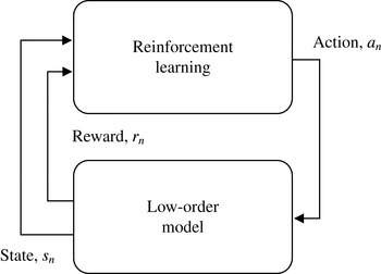
Reference Tchieu, Kanso and Newton2012). The goal of the swimmers is to swim coherently in a prescribed formation, avoiding collisions or dispersion. This is a necessary preliminary step to allow for the hydrodynamic characterization of different swimming formations in terms of energy expenditure (§ 2.5). Given the swimmers’ repertoire of possible actions and sensorial representation of the environment (referred to as states), reinforcement learning (Sutton & Barto Reference Sutton and Barto1998) allows them, through trial and error, to discover an optimal behavioural policy (i.e. a mapping between states and actions) to maintain their relative positions within the school. Each loop in figure 1 represents a single learning instance where all agents use their learned policy to select an action which alters their state through the modelled dynamics. The reward associated with the new state aids the agents in improving their policy, which eventually converges to an optimal policy.
Schematic of reinforcement learning coupled with a low-order model for swimmers in an inviscid flow. The goal of the
 $n$
th agent is encoded in the numerical reward
 $r_{n}$
, and the agent learns, through a trial-and-error process called reinforcement learning (Sutton & Barto Reference Sutton and Barto1998), how to map states
 $s_{n}$
into actions
 $a_{n}$
so as to maximize the long-term reward (§ 2.4). The system is simulated via a low-order model that takes into account swimmer–swimmer dynamics mediated by an inviscid fluid medium (Tchieu et al.
Reference Tchieu, Kanso and Newton2012).

2.1. A finite-width dipole model for hydrodynamically interacting swimmers
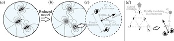
The flow field generated by individual natural swimmers possesses a complex signature that is greatly affected by the swimmers’ gait, morphology and size as well as by viscous and three-dimensional effects. The characterization of the group dynamics of hundreds of swimming bodies that resolves this level of detail is computationally beyond reach at present. Therefore, we study swimmers modelled as finite self-propelling dipoles (figure 2 a,b) immersed in an inviscid, unbounded and incompressible flow (Tchieu et al. Reference Tchieu, Kanso and Newton2012). This model reflects the fact that the far field associated with a self-propelled undulating body is dipolar to leading order (Wolfgang et al. Reference Wolfgang, Anderson, Grosenbaugh, Yue and Triantafyllou1999). The finite dipole model represents a drastic idealization of a swimmer since it abstracts from morphological and kinematic traits, is massless and therefore disregards the inertia of a solid body and does not account for three-dimensional and viscous effects such as separation and vortex shedding. Nevertheless, it does capture to first order the flow coupling among self-propelled bodies that are sufficiently spaced apart (more than one body length as estimated in Tchieu et al. (Reference Tchieu, Kanso and Newton2012)), and it is computationally effective. Bearing in mind its limitations, the dipole model is instrumental to qualitative computational investigations of fish schooling. Finally, we emphasize that self-propelled agents are distinct from agents that are towed with a certain velocity. In agent-based models the latter are usually employed, but these do not correspond to self-propelled animals responding to nonlinear interactions with the flow field.
Streamlines of (a) inviscid swimmers translating in a potential flow and (b) the finite dipole approximation of the swimmers (Tchieu et al. Reference Tchieu, Kanso and Newton2012). Shown in (c) is the detailed view of a single finite dipole, while (d) illustrates the state representation of an individual dipole swimmer attempting to follow a translating lattice point (§ 2.4).

The basis of this low-order model is depicted in figure 2. In a system of
 $N$
dipole swimmers, a dipole located at
 $\boldsymbol{x}_{n}$
(
 $n=1,2,\ldots ,N$
) is decomposed into two vortices located at
 $\boldsymbol{x}_{n}^{l}$
and
 $\boldsymbol{x}_{n}^{r}$
with circulation strengths
 ${\it\Gamma}_{n}^{l}$
and
 ${\it\Gamma}_{n}^{r}$
, separated by a constant distance
 $\ell$
. The dipole swimmer travels with a bearing defined by
 ${\it\alpha}_{n}$
, as depicted in figure 2(c). Each finite dipole swimmer can change its vortex strength as a means of controlling its bearing and speed. Following Tchieu et al. (Reference Tchieu, Kanso and Newton2012), the equations of motion of
 $N$
self-propelled interacting finite dipoles are modified to allow each dipole to change its individual bearing and speed while simultaneously affecting the flow. Note that this model is different from the one used by Chate et al. (Reference Chate, Ginelli, Gregoire, Peruani and Raynaud2008) in that the generated flow field affects the bearing of swimmers and that the swimmers directly change the flow field when performing actions. We also note that the value
 $\ell$
can be related to a characteristic width
 $D$
of the swimmer by matching the far-field dipolar strength of a body moving in an inviscid fluid to that of a finite dipole, resulting in
 $\ell =D/(2\sqrt{2{\rm\pi}})$
. To proceed, a point
 $\boldsymbol{x}$
is mapped to the complex
 $z$
-plane such that
 $\boldsymbol{x}=(x,y)\mapsto z=x+\text{i}y$
, where
 $\text{i}=\sqrt{-1}$
. Therefore, given the position of a dipole
 $\boldsymbol{x}_{n}\mapsto z_{n}$
, its two vortices of strengths
 ${\it\Gamma}_{n}^{l}$
and
 ${\it\Gamma}_{n}^{r}$
, separated by a constant distance
 $\ell$
, are located at
 $$\begin{eqnarray}z_{n}^{l}=z_{n}+\frac{\text{i}\ell \text{e}^{\text{i}{\it\alpha}_{n}}}{2}\quad \text{and}\quad z_{n}^{r}=z_{n}-\frac{\text{i}\ell \text{e}^{\text{i}{\it\alpha}_{n}}}{2},\end{eqnarray}$$
respectively (see figure 2). The equations of motion derived from Tchieu et al. (Reference Tchieu, Kanso and Newton2012) that govern the system of
 $N$
finite dipoles are modified to read
 $$\begin{eqnarray}\displaystyle & \displaystyle \dot{\overline{z}}_{n}=\frac{({\it\Gamma}_{n}^{l}+{\it\Gamma}_{n}^{r})\text{e}^{-\text{i}{\it\alpha}_{n}}}{4{\rm\pi}\ell }+\frac{w_{n}^{o}(z_{n}^{l})+w_{n}^{o}(z_{n}^{r})}{2}, & \displaystyle\end{eqnarray}$$
 $$\begin{eqnarray}\displaystyle & \displaystyle \dot{{\it\alpha}}_{n}=\frac{{\it\Gamma}_{n}^{l}-{\it\Gamma}_{n}^{r}}{2{\rm\pi}\ell ^{2}}+\frac{\text{Re}[(w_{n}^{o}(z_{n}^{r})-w_{n}^{o}(z_{n}^{l}))\text{e}^{\text{i}{\it\alpha}_{n}}]}{\ell }, & \displaystyle\end{eqnarray}$$
 $\text{Re}[\cdot ]$
denotes the real part of a complex expression and
 $$\begin{eqnarray}w_{n}^{o}(z)=\mathop{\sum }_{j\neq n}^{N}\frac{1}{2{\rm\pi}\text{i}}\left(\frac{{\it\Gamma}_{j}^{l}}{z-z_{j}^{l}}-\frac{{\it\Gamma}_{j}^{r}}{z-z_{j}^{r}}\right)\end{eqnarray}$$
is the interaction term due to all other dipoles in the environment. We emphasize that the first terms of (2.2a
) and (2.2b
) correspond to the dipole self-induced velocity and bearing rate when no other swimmers or background flow are present. Therefore, these terms relate to the ability of an agent to affect its own speed and bearing. Moreover, it is worth noting that the swimming speed is directly proportional to the dipolar circulation strength and inversely proportional to the swimmers’ size
 $D$
through
 $\ell$
. This is consistent with the fact that for a fixed amount of circulation, a small fish swims faster than a large one.
The set of five actions available to each dipole swimmer (represented by a triangle of width
 $D=2\ell \sqrt{2{\rm\pi}}$
pointing in the direction of travel), with each action mapped to the integer set
 $a_{n}=\{1,2,3,4,5\}$
: (a) travelling straight at the nominal speed
 $v^{0}$
(
 $a_{n}=1$
); (b) travelling straight at a slower speed
 $v^{-}$
(
 $a_{n}=2$
); (c) travelling straight at a faster speed
 $v^{+}$
(
 $a_{n}=3$
); (d) making a left turn at a specified turn radius
 ${\it\rho}_{T}$
(
 $a_{n}=4$
); and (e) making a right turn with turn radius
 ${\it\rho}_{T}$
(
 $a_{n}=5$
). In each panel we also show the streamlines demonstrating how a swimmer affects the background flow field in the absence of all other dipole swimmers.

We stress the fact that the dipole model allows us to evolve the system in time by actually solving the Euler equations for an incompressible inviscid flow, and so the presence of a liquid environment is not simplistically modelled through ad hoc local interaction rules. The major advantage of this formulation is that it provides a neat distinction between social and hydrodynamic effects, unlike previous modelling approaches.
2.2. Swimming gaits and manoeuvring through circulation change
We extend the original finite dipole model to equip each swimmer with a set of gaits or actions, as depicted in figure 3. A swimmer can travel forward at three distinct speeds,
 $v^{0}$
(nominal speed),
 $v^{-}=v^{0}-v^{A}$
(slow) and
 $v^{+}=v^{0}+v^{A}$
(fast), and can turn left or right with turn radius
 ${\it\rho}^{T}$
while travelling at speed
 $v^{0}$
. These actions are realized by allowing each dipole swimmer to instantaneously adjust its vortex circulations
 ${\it\Gamma}_{n}^{l}$
and
 ${\it\Gamma}_{n}^{r}$
. The five actions, mapped to integer values, adjust the circulation according to the rule
 $$\begin{eqnarray}\text{if}\quad \left\{\begin{array}{@{}lcl@{}}\displaystyle a_{n}=1:\text{ travel straight at }v^{0} & \longrightarrow & {\it\Gamma}_{n}^{l}={\it\Gamma}_{n}^{r}={\it\Gamma}^{0},\\ \displaystyle a_{n}=2:\text{ travel straight at }v^{-} & \longrightarrow & {\it\Gamma}_{n}^{l}={\it\Gamma}_{n}^{r}={\it\Gamma}^{0}-{\it\Gamma}^{A},\\ \displaystyle a_{n}=3:\text{ travel straight at }v^{+} & \longrightarrow & {\it\Gamma}_{n}^{l}={\it\Gamma}_{n}^{r}={\it\Gamma}^{0}+{\it\Gamma}^{A},\\ \displaystyle a_{n}=4:\text{ turn left with radius }{\it\rho}^{T} & \longrightarrow & {\it\Gamma}_{n}^{l}={\it\Gamma}^{0}+{\it\Gamma}^{T},~{\it\Gamma}_{n}^{r}={\it\Gamma}^{0}-{\it\Gamma}^{T},\\ \displaystyle a_{n}=5:\text{ turn right with radius }{\it\rho}^{T} & \longrightarrow & {\it\Gamma}_{n}^{l}={\it\Gamma}^{0}-{\it\Gamma}^{T},~{\it\Gamma}_{n}^{r}={\it\Gamma}^{0}+{\it\Gamma}^{T},\end{array}\right.\end{eqnarray}$$
where
 ${\it\Gamma}^{0},{\it\Gamma}^{A},{\it\Gamma}^{T}>0$
. The nominal vortex strength
 ${\it\Gamma}^{0}$
is related to the cruise velocity
 $v^{0}$
and the characteristic size
 $\ell$
through
 ${\it\Gamma}^{0}=2{\rm\pi}\ell v^{0}$
.
The additional circulations
 $\pm {\it\Gamma}^{A}$
and
 $\pm {\it\Gamma}^{T}$
due to travelling fast or slow and turning right or left are fixed by the swimming parameters
 $v^{0}$
,
 $v^{A}$
and
 ${\it\rho}^{T}$
. These values are related to the nominal circulation by
 $$\begin{eqnarray}\displaystyle & \displaystyle {\it\Gamma}^{A}=\left(\frac{v^{A}}{v^{0}}\right){\it\Gamma}^{0}, & \displaystyle\end{eqnarray}$$
 $$\begin{eqnarray}\displaystyle & \displaystyle {\it\Gamma}^{T}=\left(\frac{{\it\rho}^{T}}{\sqrt{2{\rm\pi}}\ell }\right)^{-1}{\it\Gamma}^{0}. & \displaystyle\end{eqnarray}$$
We emphasize that the use of five actions is a simplification of the movements of naturally occurring swimmers, which are characterized by a large number of kinematic degrees of freedom, so that swimmers have the ability to fine tune their gaits in response to environmental cues. However, the use of a small number of actions drastically reduces the computational costs associated with identifying an optimal behavioural policy through reinforcement learning, hence our choice to equip the agents with a limited repertoire of gaits.
2.3. The Aoki–Couzin behavioural model with hydrodynamics interactions
We examine how the classical Aoki–Couzin model (Aoki Reference Aoki1982; Couzin et al. Reference Couzin, Krause, James, Ruxton and Franks2002) with a priori defined interaction rules would perform in the presence of hydrodynamics. In particular, we considered the so-called ‘dynamically parallel school’ and ‘highly parallel school’ behavioural rules, as detailed in (Couzin et al. Reference Couzin, Krause, James, Ruxton and Franks2002).
In the Aoki–Couzin model, collective behaviour emerges due to three a priori specified rules among agents: each agent tries to avoid collision with neighbours, aligns to the moving direction of the agents contained in a larger neighbourhood and, finally, tends to approach the agents of an even larger neighbourhood. Given these three rules, each agent first computes its desired direction and then turns in accordance with that direction (Couzin et al. Reference Couzin, Krause, James, Ruxton and Franks2002). By varying the size of the interaction regions, qualitatively different behaviours can be observed. In table 1, we summarize the radii characteristic of the ‘dynamically parallel school’ and ‘highly parallel school’, as detailed in Couzin et al. (Reference Couzin, Krause, James, Ruxton and Franks2002) and used here.
Radii of zones of interaction relative to the ‘dynamically parallel school’ and ‘highly parallel school’ behaviours as detailed in Couzin et al. (Reference Couzin, Krause, James, Ruxton and Franks2002); the radii are normalized by
 $\ell$
.

In order to cast the Aoki–Couzin model in the present dipole framework, each dipole agent determines its desired direction
 ${\it\alpha}_{\mathit{desired}}$
by following the specifications of Couzin et al. (Reference Couzin, Krause, James, Ruxton and Franks2002), and then adjusts its vortex circulations as follows:
 $$\begin{eqnarray}\left.\begin{array}{@{}c@{}}\displaystyle \dot{{\it\alpha}}_{\mathit{desired}}=\frac{{\it\alpha}_{\mathit{desired}}-{\it\alpha}_{0}}{{\it\tau}}\\ \displaystyle {\it\Gamma}_{\mathit{add}}={\rm\pi}\ell ^{2}(\dot{{\it\alpha}}_{\mathit{desired}}-\dot{{\it\alpha}}_{0})\\ \displaystyle {\it\Gamma}^{l}={\it\Gamma}^{l}+{\it\Gamma}_{\mathit{add}}\\ \displaystyle {\it\Gamma}^{r}={\it\Gamma}^{r}-{\it\Gamma}_{\mathit{add}}\end{array}\right\}\end{eqnarray}$$
where
 ${\it\tau}$
,
 ${\it\alpha}_{0}$
and
 $\dot{{\it\alpha}}_{0}$
are, respectively, the simulation’s time step and the agent’s current bearing and bearing rate. Computing the new
 ${\it\Gamma}^{r}$
and
 ${\it\Gamma}^{l}$
corresponds to adapting the gaits to match exactly the desired bearings, assuming the absence of all other swimmers. Once the circulations of the individual dipoles are determined, the system of
 $N$
swimmers is evolved by accounting for hydrodynamic coupling via the governing equations (2.1)–(2.3).
The behaviour of this model in the presence of hydrodynamic interactions is examined in § 3.2.
2.4. Reverse engineering of dynamic interaction rules via reinforcement learning
Swimmers are modelled as finite-width dipoles with varying circulation strength. Their presence and actions affect the flow field and, in turn, all other swimmers. Because of this highly nonlinear coupling, it is virtually impossible to handcraft local interaction rules that allow the dipoles to coherently swim in any predefined, finite-size schooling arrangement. Therefore agent-based models, with a priori defined rules, cannot help us to assess the hydrodynamic properties of different schooling configurations. With this in mind, we employ a reverse engineering approach to obtain the interaction rules among swimmers. We specify for the agents the goal of maintaining a given geometric arrangement and employ a reinforcement learning technique to identify an appropriate interaction policy. This approach relies on four key components: the reward that encodes the agent’s goal; the state that formalizes what the dipole can sense of the surrounding environment; the actions, i.e. the repertoire of gaits at each swimmer’s disposal (§ 2.2); and, finally, a learning strategy based on trial and error.
In this study we employ a particular reinforcement learning technique, namely the one-step
 $Q$
-learning algorithm (Sutton & Barto Reference Sutton and Barto1998). Besides its algorithmic simplicity,
 $Q$
-learning has been proven to converge to an optimal behavioural policy for finite Markov decision processes (Watkins & Dayan Reference Watkins and Dayan1992). In this setting, the swimming agent explores the environment and its experience is represented by the tuple
 $\langle s_{n},a_{n},r_{n},s_{n}^{\prime }\rangle$
, where
 $s_{n}^{\prime }$
is the next state given the action
 $a_{n}$
taken from the current state
 $s_{n}$
and
 $r_{n}$
is the corresponding reward. An agent estimates by trial and error the action-value function
 $Q_{n}(s_{n},a_{n})$
, i.e. the expected long-term reward for taking action
 $a_{n}$
given the state
 $s_{n}$
(a schematic of this approach is depicted in figure 1). The action-value function
 $Q_{n}$
can be understood as a table or a matrix in which for every state–action entry the corresponding expected reward (estimated through the reward history) is stored. This table is consulted by the agent whenever an action has to be taken, and it is continuously updated as the system evolves. Therefore
 $Q_{n}$
encodes the swimmers’ adaptive decision-making intelligence, and the corresponding behaviour is determined by choosing from
 $Q_{n}$
, with probability
 $1-{\it\epsilon}$
, the best action
 $a_{n}$
such that
 $a_{n}\rightarrow \max _{a_{n}}Q_{n}(s_{n},a_{n})$
from the current state
 $s_{n}$
(an
 ${\it\epsilon}$
-greedy selection scheme). The
 ${\it\epsilon}$
-probability of choosing a non-optimal action allows the agent to explore new state–action
 $(s_{n},a_{n})$
pairs (Sutton & Barto Reference Sutton and Barto1998). Therefore, reinforcement learning intrinsically accounts for noise through
 ${\it\epsilon}$
, which can be related to the noise of natural schooling systems. Here, we use a shared policy approach among all swimmers to accelerate the learning process; thus
 $Q_{n}=Q$
and all agents update
 $Q$
based on their personal experience. At every learning time interval
 ${\it\delta}t$
, the swimmers update the action-value function according to
 $Q(s_{n},a_{n})=Q(s_{n},a_{n})+{\it\varphi}({\rm\Delta}Q)_{n}$
for
 $n=1,\ldots ,N,$
where
 $0\leqslant {\it\varphi}\leqslant 1$
is the learning rate and
 $({\rm\Delta}Q)_{n}=r_{n}+{\it\gamma}\max _{a_{n}}Q(s_{n}^{\prime },a_{n})-Q(s_{n},a_{n})$
, with
 $0\leqslant {\it\gamma}<1$
being the discount parameter which corresponds to the weight given to past experiences. We emphasize that learning individual policies, as opposed to the shared approach employed here, may allow agents finer behavioural tuning. For example, in the case of schooling, swimmers may adapt their policies depending on their location within the group. However, it has been shown empirically that the use of a shared policy reduces the time to convergence linearly with the number of agents (Gazzola Reference Gazzola2013). In our study this entails a hundreds-fold reduction in computational cost, which is the rationale behind our choice of employing a shared approach. In the following paragraphs the definitions of reward, state and action are formalized.
Reward. Since ultimately we are interested in investigating the hydrodynamic properties associated with different schooling geometries, we must first have the dipoles learn to swim in a given formation. This is achieved by setting the goal of each swimmer as following a specified target point
 $\boldsymbol{x}_{n}^{t}$
in a predefined arrangement, as depicted in figure 2(d). This allows hundreds of self-propelled dipoles to learn how to swim coherently, a task that is beyond the reach of models based on handcrafted a priori interaction rules (in §§ 2.5 and 3.4 we detail how optimal arrangements can be obtained). The swimmer’s goal is translated mathematically into a numerical reward signal. The numerical reward is chosen to reflect how well the dipole swimmer can follow its assigned target point while doing the minimum amount of manoeuvring so that
 $r_{n}=w_{d}(1-d_{n}/\ell )+w_{a}\cdot {\it\eta}_{a}$
, where
 ${\it\eta}_{a}=0$
for travelling at
 $v_{0}$
,
 ${\it\eta}_{a}=-1$
for accelerating and turning and
 ${\it\eta}_{a}=1$
for decelerating. Weights are set to
 $w_{d}=0.9$
and
 $w_{a}=0.1$
; thus
 $\max (r_{n})=1$
. We note how the second term of
 $r_{n}$
penalizes swimmers that take unnecessary actions, while favouring those that reduce their effort by slowing down.
State. Swimmers can sense their distance
 $d_{n}=|\boldsymbol{x}_{n}^{t}-\boldsymbol{x}_{n}|$
and orientation
 ${\it\theta}_{n}=\arg (\boldsymbol{x}_{n}^{t}-\boldsymbol{x}_{n})-{\it\alpha}_{n}$
with respect to their assigned target point
 $\boldsymbol{x}_{n}^{t}$
within the school, as shown in figure 2(d). We stress the fact that the dynamics of a swimmer is not mapped onto a lattice. Swimmers are in fact free to move in the continuum two-dimensional space, while they adaptively adjust their gait in the attempt to maintain their relative position within the school. Instead, the quantities
 $d_{n}$
and
 ${\it\theta}_{n}$
are each mapped into a set of
 $L=30$
discrete states within the range
 ${\rm\Delta}d=10D$
and
 ${\rm\Delta}{\it\theta}=2{\rm\pi}$
such that
 $s_{n}=\{\min (L,\max (0,\lfloor d_{n}L/{\rm\Delta}d\rfloor )),\min (L,\max (0,\lfloor {\it\theta}_{n}L/{\rm\Delta}{\it\theta}\rfloor ))\}$
. In total, each swimmer has a state space that consists of 900 states. The choice of a target point over the sensing of the neighbours dramatically reduces the state-space dimension (the curse of dimensionality), allowing us to tackle the problem computationally. Moreover, it enables the study of structured schooling arrangements while still capturing the influence of neighbours as they directly affect each other’s dynamics through long-range hydrodynamic interactions.
Actions. Each dipole swimmer can perform five actions: it can travel forward at three distinct speeds,
 $v^{0}$
(its nominal travelling speed),
 $v^{+}=1.1v^{0}$
and
 $v^{-}=0.9v^{0}$
, or turn left or right with radius
 $r^{T}=10\ell$
while travelling at
 $v^{0}$
. These actions are realized by allowing the dipole swimmer to adjust its vortex circulations
 ${\it\Gamma}_{n}^{l}$
and
 ${\it\Gamma}_{n}^{r}$
accordingly (§ 2.2). Since for every state five different gaits are available, the overall state–action space has 4500 entries, to be stored in a table representing the action-value function
 $Q(s_{n},a_{n})$
.
An example further illustrating the working principles of reinforcement learning is reported in § 3.1.
2.5. Optimization of schooling patterns via evolution strategies
In the previous sections we established the algorithmic framework that allows self-propelled swimmers to learn how to keep their relative position within a school. We now look for optimal swimming configurations according to a desired metric (cost function), using the ‘covariance matrix adaptation evolutionary strategy’ (CMA-ES) of Hansen, Muller & Koumoutsakos (Reference Hansen, Muller and Koumoutsakos2003). The CMA-ES has been proven effective in a number of fluid mechanics and biological problems, from the optimization of gait and morphology in swimmers (Kern & Koumoutsakos Reference Kern and Koumoutsakos2006; Gazzola, van Rees & Koumoutsakos Reference Gazzola, van Rees and Koumoutsakos2012b ; van Rees, Gazzola & Koumoutsakos Reference van Rees, Gazzola and Koumoutsakos2013, Reference van Rees, Gazzola and Koumoutsakos2015) to the identification of virus traffic mechanisms (Gazzola et al. Reference Gazzola, Burckhardt, Bayati, Engelke, Greber and Koumoutsakos2009).
The CMA-ES is a stochastic optimization algorithm that samples at each generation
 $p$
parameter vectors from a multivariate Gaussian distribution
 $\mathscr{N}$
. Here each parameter vector encodes the geometric configuration of a schooling arrangement (appendix A). The covariance matrix of the distribution
 $\mathscr{N}$
is then adapted based on successful past schools, chosen according to their corresponding cost function value
 $f$
. In the present context, the CMA-ES evolves schooling configurations based on a metric of swimming effectiveness. In order to evaluate the cost function, i.e. the performance, of each school geometry, the dipole swimmers must first learn through reinforcement learning how to swim coherently in that specific arrangement. Then, after a learning period
 ${\rm\Delta}T_{\mathit{learning}}$
, the average cost function is evaluated by simulating the school for the time
 ${\rm\Delta}T_{\mathit{eval}}$
(appendix A). The value
 $f$
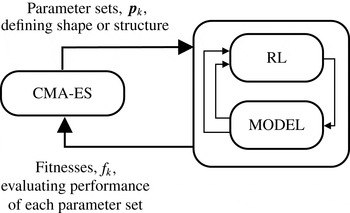
so computed is then returned to the optimizer, which uses it to select the best configurations and produce a new, more performant generation of school arrangements, until convergence to an optimal solution is achieved. This process is depicted in figure 4, while the definition of the cost function is given in the next paragraph.
Schematic of CMA-ES optimizer coupled with reinforcement learning (RL) and the low-order model. The CMA-ES dispatches
 $k=1,\ldots ,p$
parameter sets
 $\boldsymbol{p}_{k}$
defining the school configuration. The reinforcement learning framework allows agents to learn to swim in the formation characterized by
 $\boldsymbol{p}_{k}$
. In return, the CMA-ES receives a fitness
 $f_{k}$
that captures the effectiveness of collective swimming relative to each school
 $\boldsymbol{p}_{k}$
.

Cost function. Here the cost function to be minimized implements a metric of swimming effort for the entire school. The effort of an individual swimmer relative to its nominal cruise effort, i.e. its additional circulation expenditure, is defined by
 $$\begin{eqnarray}{\rm\Delta}{\it\Gamma}_{n}^{e}=\frac{1}{{\rm\Delta}T_{\mathit{eval}}}\int _{t}^{t+{\rm\Delta}T_{\mathit{eval}}}(\underbrace{|{\it\Gamma}_{n}^{l}-{\it\Gamma}_{n}^{r}|}_{\text{turning effort}}+\underbrace{{\it\Gamma}_{n}^{l}+{\it\Gamma}_{n}^{r}}_{\text{forward effort}}-2{\it\Gamma}^{0})\,\text{d}t,\end{eqnarray}$$
where
 ${\it\Gamma}^{0}$
is the nominal strength of each vortex. Hence, the cost function for the entire collection of swimmers is defined as
 $f=1/(N{\it\Gamma}^{0})\sum _{n=1}^{N}{\rm\Delta}{\it\Gamma}_{n}^{e}$
. The change in circulation can be related to the production of vorticity involved in accelerations or turning manoeuvres of the swimmers and, therefore, to the swimming effort. We also note for future reference that
 $f=0$
corresponds to cruise swimming of isolated dipoles.
3. Results
3.1. Learning process for an individual dipole swimmer
Despite the formalism, the working principles of reinforcement learning are rather simple. We illustrate them here with the aid of a simple but representative problem, before proceeding further.
We consider a dipole whose goal is to follow a prescribed trajectory. The trajectory is represented as a target point
 $\boldsymbol{x}^{t}$
that moves by alternating straight runs and random turns of fixed radius
 ${\it\rho}^{T}$
. The dipole is aware at all times of its own bearing
 ${\it\alpha}$
and position
 $\boldsymbol{x}$
as well as of the target position
 $\boldsymbol{x}^{t}$
. At regular intervals
 ${\it\delta}t$
, the agent is faced with the problem of choosing whether to turn left or right, accelerate, slow down or keep straight in order to accurately follow the target point. The dipole has not been instructed how to act given its relative position to the target, i.e. no a priori local rules are enforced. Instead, at every time step the swimmer estimates its relative distance
 $d$
and orientation
 ${\it\theta}$
with respect to
 $\boldsymbol{x}^{t}$
, as illustrated in figure 2(d). This is equivalent to determining the state
 $s$
, i.e. the agent’s current situation. Since the intelligence or behaviour of the swimmer is encoded as a multidimensional table or matrix, the continuous values of
 $d$
and
 ${\it\theta}$
are discretized into a number of integer values, as described in § 2.4. Once the state matrix entry is determined, the agent can consult the expected rewards stored in the matrix associated with taking each of the five aforementioned actions
 $a$
. These values
 $Q(s,a)$
are constantly updated by the dipole and represent its past experience; initially they are all set to zero. At this point the agent chooses with probability
 $1-{\it\epsilon}$
the best action, i.e. the one with the largest
 $Q(s,a)$
value, and after pursuing it the new distances
 $(d^{\prime },{\it\theta}^{\prime })$
from the target are estimated, defining the new state
 $s^{\prime }$
. Moreover, based on
 $d^{\prime }$
, the reward
 $r$
is assigned to the dipole. The policy is then improved by discounting the old estimate of the expected reward
 $Q(s,a)$
and complementing it with the new information
 $r$
according to the update rule described in § 2.4. This process is repeated indefinitely until convergence to an optimal behavioural policy.
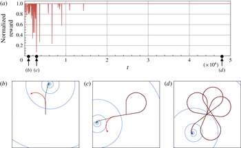
The evolution of the swimmer’s reward over time is shown in figure 5(a), and examples of the agent trajectories during the learning process are given in figure 5(b–d). The process of improving the policy can be seen in figure 5(a), where, after an initial transient, the agent progressively learns how to maximize its numerical reward by accurately following
 $\boldsymbol{x}^{t}$
. In figure 5(b), the swimmer fails rather quickly, as demonstrated by its path diverging from the target path at the first turn. Subsequently, in figure 5(c), the swimmer follows adequately for a longer time before failing, and in figure 5(d) the swimmer learns a policy that allows it to follow a pseudo-random path indefinitely.
A single agent learns to optimally follow a moving target point
 $\boldsymbol{x}^{t}$
. Shown in (a) is the time evolution of the agent’s reward normalized by its maximum attainable value, based on the reward definition given in § 2.4. Panels (b–d) correspond, respectively, to non-adaptive, intermediate-adaptive and well-adaptive learning stages. The starting times for panels (b–d) are marked on the
 $x$
-axis of (a). Black dashed and solid red lines correspond, respectively, to the trajectories of the agent (green triangle) and the target point (red dot). Instantaneous streamlines (blue lines) are displayed for reference. Simulations are run in the domain
 $[0,1]\times [0,1]$
with
 $\ell =3\times 10^{-3}$
,
 $v^{0}=5\ell$
,
 $v^{A}=0.1v^{0}$
,
 ${\it\rho}^{T}=10\ell$
,
 ${\it\delta}t=0.1$
,
 ${\it\varphi}=0.01$
,
 ${\it\gamma}=0.98$
and
 ${\it\epsilon}=0.01$
. The notation is defined in § 2 and appendix A.

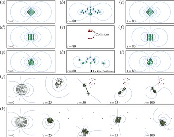
Swimming configurations for 16 dipole swimmers at specified times: (a,d,g) initial/desired configurations; (b,e,h) non-adaptive configurations; (c,f,i) adaptive (with policy learned from reinforcement learning) configurations. Red dipole swimmers have experienced a collision (after which they no longer move). Instantaneous streamlines (blue lines) are displayed for reference. Dipole swimmers are initialized on a diamond lattice in (a–c), a square lattice in (d–f) and randomly in a circular region of radius of
 $17.5\ell$
in (g–i). In all initial configurations, a minimum interdipole spacing of
 $10\ell$
is enforced. Also shown are the time evolutions of a school of 100 agents obeying (j) ‘dynamically parallel group’ and (k) ‘highly parallel group’ models (Couzin et al.
Reference Couzin, Krause, James, Ruxton and Franks2002) enhanced with hydrodynamic interactions. Simulations are run in the domain
 $[0,1]\times [0,1]$
with
 $\ell =5\times 10^{-4}$
,
 $v^{0}=5\ell$
,
 $v^{A}=0.1v^{0}$
,
 ${\it\rho}^{T}=10\ell$
,
 ${\it\delta}t=0.1$
,
 ${\it\varphi}=0.01$
,
 ${\it\gamma}=0.98$
and
 ${\it\epsilon}=0.01$
. The notation is defined in § 2 and appendix A.

3.2. Classical agent-based models versus learning agents in the presence of hydrodynamics
We first show that prescribed schooling patterns, including the diamonds and squares which have been proposed as favourable schooling patterns (Weihs Reference Weihs1973), are not robustly maintained without an adaptive dynamic response of the swimmers to the flow field. In figure 6 we display the results of 16 swimming agents attempting to school in several formations initialized (at
 $t=0$
) as shown in figure 6(a,d,g). These initial patterns are characterized by diamond-like, square-like and random arrangements. With a prespecified forward swimming gait, the relative locations of swimmers will result in varying hydrodynamic loads, thus implying a dynamic rearrangement of the swimmers. Indeed, when the agents are assigned a specified swimming configuration, the simulated swimmers diverge from their relative positions and are prone to collisions with their neighbours due to flow-mediated interactions, which is consistent with the findings of Tchieu et al. (Reference Tchieu, Kanso and Newton2012). As shown in figure 6(b) at
 $t=80$
, no collisions occur in the diamond-like configuration, but the swimmers are strained apart substantially. In figure 6(e) it can be seen that initializing with the square arrangement causes all agents to collide, while figure 6(h) shows that random configurations lead simultaneously to straining and collision effects. A qualitative hydrodynamic explanation for the disruption of square-like and diamond-like formations is provided in § 3.4 and figure 10. From figure 6(c,f,i) we see that schooling patterns can be maintained by swimmers through an adaptive modification of their swimming gaits that accounts for hydrodynamic interactions using a reinforcement learning algorithm. Therefore, through reinforcement learning the agents learn to adjust their swimming gaits to compensate for the varying hydrodynamic loads typical of a liquid environment. This can be related to the noisy environments and the corresponding response of swimmers in natural schooling systems.
We note that while the stability of diamond and square configurations has also been investigated by Tsang & Kanso (Reference Tsang and Kanso2013), our approach is fundamentally different. In fact, Tsang & Kanso (Reference Tsang and Kanso2013) considered infinite, doubly periodic lattices of dipoles characterized by a single gait. The dipoles are then arranged so that the resulting flow field passively stabilizes the lattice, removing altogether the need to respond to varying loads by adapting swimming gaits, and the associated energetic costs. Here, the assumption of infinite schools is discarded in favour of a more realistic description. As a consequence, passive stabilization due to a stationary global flow field is no longer an option, hence the introduction of varying gaits and adaptive decision-making. Therefore, our approach complements the results of Tsang & Kanso (Reference Tsang and Kanso2013), allowing us to study the hydrodynamic and energetic features associated with arbitrarily shaped, finite-size schools.
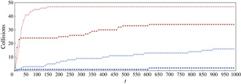
Comparison of the quantitative response of the Aoki–Couzin model with and without hydrodynamic interactions in terms of the number of agent collisions over time. A collision is detected whenever the distance between two agents is less than
 $2\ell$
. Red and blue correspond, respectively, to the ‘dynamically parallel group’ and ‘highly parallel group’ behavioural rules (Couzin et al.
Reference Couzin, Krause, James, Ruxton and Franks2002). Blank and solid circles refer, respectively, to simulations with and without hydrodynamics.

We also investigated the dynamics of the Aoki–Couzin behavioural model (Aoki Reference Aoki1982; Couzin et al. Reference Couzin, Krause, James, Ruxton and Franks2002) in the presence of hydrodynamic interactions (§ 2.3). This model relies on a priori handcrafted local interaction rules among agents and does not explicitly account for the flow environment during the decision-making process. The time evolutions of a school of 100 agents obeying ‘dynamically parallel group’ and ‘highly parallel group’ behavioural rules (Couzin et al. Reference Couzin, Krause, James, Ruxton and Franks2002) are shown in figure 6(j,k). We find that the swimmers experience substantial straining and collisions, due to the hydrodynamic coupling. This behaviour is a drastic departure from the schooling patterns observed when employing the original models (Couzin et al. Reference Couzin, Krause, James, Ruxton and Franks2002). Indeed, the number of collisions increases by 40 % and 700 % in, respectively, the ‘dynamically parallel group’ and ‘highly parallel group’ models in the presence of hydrodynamics (figure 7). These findings emphasize the role of the environment, especially in a hydrodynamic setting in which all agents are doubly connected through the flow. The fact that the nonlinear response of the hydrodynamic system cannot be anticipated makes the definition of interaction rules by hand cumbersome, tedious and, ultimately, not robust.
Agent-based models with a priori specified rules, such as the ones considered herein, are characterized by a large parameter space (size of each zone, attraction and repulsion weights, time step etc.), and their results are known to be sensitive to these settings. In this study we have not explored the full parameter space and so cannot rule out the possibility that particular parameter combinations may allow dipole swimmers to maintain structured arrangements or exhibit robust schooling dynamics. Nevertheless, the present investigation raises two key issues. First, the introduction of the flow environment modifies the dynamics associated with classical agent-based model settings. This implies that to reproduce the behaviour observed for a given instance of the Aoki–Couzin model, a new set of parameters has to be discovered. Since zone sizes and attractive and repulsive forces have a well-defined ‘social’ meaning, the presence of the fluid affects these quantities and alters the nature of social interactions. Therefore, the characterization of social traits cannot be prescinded from accounting for the environment. Second, the sensitivity of classical models to parameter settings supports the need for rigorous, automatic procedures for identifying local rules in the context of collective behaviour. Indeed, we have been unable to handcraft or derive through a direct optimization process any parameter set that would enable dipole swimmers to maintain a structured schooling formation, whereas this was readily achieved through the reinforcement learning framework. We reiterate that this finding does not represent a mathematical proof that handcrafted a priori models do not lead robustly to schooling, but it strongly highlights the need for computational methods that can guide the systematic exploration of the models’ parameter space.
3.3. Optimal internal structure of a school of dipole swimmers
Since it has been suggested that diamond lattices embedded in an infinite school are energetically favourable (Weihs Reference Weihs1973; Tsang & Kanso Reference Tsang and Kanso2013), we first characterize in terms of collective effort only the internal structure of schooling formations, disregarding edge effects related to the finite size of the school. The swimming effort of an individual is quantified by the variation of its dipole strength from a nominal value,
 ${\rm\Delta}{\it\Gamma}_{n}^{e}$
(see § 2.5). This effort changes during swimming, according to the reinforcement learning algorithm, to overcome hydrodynamic noise. We therefore optimize the bulk school structure so as to minimize the cost function
 $f$
defined as the linear sum of the efforts of all the swimmers in the group (§ 2.5), with
 $f=0$
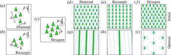
corresponding to cruise swimming of isolated swimmers. We consider three different parameterizations for generalized internal structure: (a) diamond, (b) rectangle and (c) hexagon configurations, as depicted in figure 8(a–c). The parameter
 ${\it\beta}$
characterizes the angle between the swimming direction and the axis defining the lattice structure (see the insets of figure 8
a–c). The hexagon formations constitute a subset of diamond formations, with the additional restriction that swimmers should be equidistant to their nearest neighbours. To minimize edge effects, we generate a circular shape and fill it with a lattice of
 $N\approx 200$
agents. Collective effort is evaluated only for the interior agents, and our criteria selects for the 50 agents closest to the centre of the school.
The starting configurations are shown in figure 8(d–f), while the corresponding optimal solutions are displayed in figure 8(g–i). The swimmers form striated patterns and get closely packed with one another in their travelling direction while separating as far as possible (given the bounds of the optimization search space) in the orthogonal direction. The packing in the direction of travel is limited by the capacity of the agents to stay in formation due to the strong flow-mediated interactions.
For the hexagon case (equidistant neighbours), from a starting configuration that is slightly detrimental to the school (
 $f_{1}=0.001$
), the optimizer finds a configuration that offers no added benefit to the collective, as the fitness of the case shown in figure 8(i) is
 $f_{\mathit{best}}\approx 0$
. We conclude that the constraint of equidistant swimmers does not allow the agents to pack in the direction of travel and thus is not favourable to reducing circulation expenditure.
The three different parameterizations for the internal structure of the school: we choose to investigate (a) diamond configurations parameterized by
 $\boldsymbol{p}=\{b,h,{\it\beta}\}$
, (b) rectangular configurations parameterized by
 $\boldsymbol{p}=\{b,h,{\it\beta}\}$
and (c) hexagon configurations parameterized by
 $\boldsymbol{p}=\{b,{\it\beta}\}$
. In (c), all agents are equidistant to their nearest neighbours. The angle
 ${\it\beta}$
represents the difference in direction of travel with respect to the axis defining the structure. Panels (d–f) show the initial guesses, where the fitnesses
 $f\approx 0$
, and panels (g–i) show the best optimized solutions for the parameters of the internal structure defined according to (a–c). The population size is
 $p=100$
. Streamlines are shown in blue. The optimal parameters are (g)
 $\boldsymbol{p}_{\mathit{best}}=\{49.70\ell ,2.55\ell ,0.02\}$
, (h)
 $\boldsymbol{p}_{\mathit{best}}=\{45.90\ell ,5.20\ell ,-0.03\}$
and (i)
 $\boldsymbol{p}_{\mathit{best}}=\{37.25\ell ,0.52\}$
, corresponding to the fitnesses
 $f_{\mathit{best}}=-0.175,-0.184$
and 0, respectively. Swimmers tend to form striated patterns in diamond and rectangular configurations; in the case where dipole swimmers are required to be equidistant from one another, there is no apparent hydrodynamic benefit from staying in the collective. Simulations are run in a
 $[0,1]\times [0,1]$
box with
 $\ell =5\times 10^{-4}$
(or
 $\ell =1\times 10^{-4}$
),
 $v^{0}=5\ell$
,
 ${\it\rho}^{T}=10\ell$
,
 ${\it\delta}t=0.1$
,
 ${\it\varphi}=0.01$
,
 ${\it\gamma}=0.98$
and
 ${\it\epsilon}=0.01$
. The notation is defined in § 2 and appendix A. We note that the model relies on the assumption that swimmers are separated more than one characteristic length
 $\ell$
from one another (Tchieu et al.
Reference Tchieu, Kanso and Newton2012). This condition is met here with the minimum distance of
 $2.55\ell$
for (g), corresponding to the spacing
 $b$
in our parameterization. This implies that swimmers could pack even tighter, but such a scenario is found to be suboptimal.

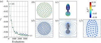
(a) Evolution of the cost function
 $f$
versus the number of cost function evaluations. The population size per generation is
 $p=100$
; blue and green lines correspond, respectively, to the best solution in the current generation and the best solution ever. Also shown are the school formations corresponding to (b) the starting search point (
 $\boldsymbol{p}_{1}=\{3,1,1,1.57\}$
,
 $f_{1}=-0.005$
) and (c) the best point (
 $\boldsymbol{p}_{\mathit{best}}=\{1.35,0.5,1.98,2.42\}$
,
 $f_{\mathit{best}}=-0.067$
). The additional circulation change is computed for each swimmer and coloured accordingly. Simulations are run in the domain
 $[0,1]\times [0,1]$
with
 $\ell =5\times 10^{-4}$
,
 $v^{0}=5\ell$
,
 ${\it\rho}^{T}=10\ell$
,
 ${\it\delta}t=0.1$
,
 ${\it\varphi}=0.01$
,
 ${\it\gamma}=0.98$
and
 ${\it\epsilon}=0.01$
. All configurations correspond to a simulation time of
 $t=100$
. The notation is as defined in § 2 and appendix A. Panel (d) shows streamlines of the starting search point and panel (e) the best solution configuration. Given in panel (f) is a detailed view of the dashed box in (e), with the dipole swimmers represented as black dots. As can be seen from (f), it is advantageous for the dipole swimmers to line up in striated patterns to aid in creating a favourable flow in the direction of travel. Indeed, the higher streamline density in this direction is the footprint of a stronger longitudinal velocity field. We note that the dipole model relies on the assumption that swimmers are separated more than one characteristic length
 $\ell$
from one another (Tchieu et al.
Reference Tchieu, Kanso and Newton2012). This condition is met here with a minimum distance of
 $1.35\ell$
(first entry of the parameter vector
 $\boldsymbol{p}_{\mathit{best}}$
). This implies that swimmers could pack even tighter, but such a scenario is found to be suboptimal.

The results reported in this section may be viewed in the light of recent experiments that systematically investigated the thrust, power and efficiency performance of two side-by-side (Dewey et al.
Reference Dewey, Quinn, Boschitsch and Smits2014) and in-line pitching airfoils (Boschitsch, Dewey & Smits Reference Boschitsch, Dewey and Smits2014). In the side-by-side case (Dewey et al.
Reference Dewey, Quinn, Boschitsch and Smits2014), it is found that the performances of individual airfoils are always anticorrelated, except for perfectly in-phase or out-of-phase actuation (which may not be realistic or robust in a schooling system). This arrangement entails an overall constant system efficiency and the generation of a net torque, which needs to be compensated for in stable schooling arrays. In the context of our study, these results suggest no foreseeable benefits associated with parallel swimming dipoles. Indeed, the striated patterns identified tend to minimize anticorrelation effects, by stretching lateral spacings as much as possible, effectively decoupling parallel dipoles. The case of in-line pitching airfoils is more complex. For small spacings
 $s/\ell <0.5$
(where
 $s$
is the linear coordinate in the direction of travel and
 $\ell$
is the airfoil chord), the performances of the leading and trailing airfoils are anticorrelated. For larger spacings, on the other hand, only the trailing body is affected and the vortex shedding from the leading airfoil plays a prominent role in the observed dynamics. Extrapolating to multiple airfoils, we might expect small spacings to be suboptimal. In fact, owing to the strong anticorrelation, every airfoil would experience both enhancing and disruptive effects. A larger spacing would instead allow, under the appropriate phase lag, all airfoils to benefit from flow coupling. The dipole model does not account explicitly for vortex shedding. As a consequence, there is no phase lag or cutoff separation distance that controls the interactions of the leading and trailing dipoles. Nevertheless, the optimization process discards configurations characterized by small spacing, since the strong anticorrelated dipole interaction poses control and learning problems and increases the swimming effort. Dipoles settle for larger spacing (
 $s/\ell \geqslant 2.55$
in figure 8,
 $s/\ell \geqslant 1.35$
in figure 9) to weaken anticorrelation effects, allowing for better stability and reduced effort, consistent with the above observations. We conclude that our findings, within the limits of our modelling approach, qualitatively capture the salient features associated with two-body swimming interactions (Boschitsch et al.
Reference Boschitsch, Dewey and Smits2014; Dewey et al.
Reference Dewey, Quinn, Boschitsch and Smits2014).
3.4. Optimal shape of a school of dipole swimmers
We proceed by optimizing for the collective swimming effort
 $f$
of the school configuration as a whole, where both internal structure and edge effects compete simultaneously. We initialize a school formation by arranging
 $N=100$
swimmers in a prescribed shape so as to maximize the distance from each other as well as from the shape boundary (appendix A). The schooling arrangement is specified by four parameters
 $\boldsymbol{p}=\{k_{1},k_{2},{\it\phi}_{1},d_{\mathit{avg}}\}$
, where
 $k_{1}$
,
 $k_{2}$
and
 ${\it\phi}_{1}$
characterize its shape and
 $d_{\mathit{avg}}$
determines its area,
 $A=N\cdot d_{\mathit{avg}}^{2}$
. Again the parameters corresponding to the optimal schooling arrangement are identified through the CMA-ES algorithm (§ 2.5) by minimizing
 $f$
, with
 $f=0$
corresponding to cruise swimming of isolated swimmers.
The course of the stochastic optimization is shown in figure 9(a). The schooling arrangement evolves from the initial circular shape in figure 9(b) to the optimal ‘hourglass’ solution of figure 9(c), reminiscent of shapes observed in nature for medium-sized schools (Misund, Aglen & Fronaes Reference Misund, Aglen and Fronaes1995; Parrish, Viscido & Grünbaum Reference Parrish, Viscido and Grünbaum2002). The ‘hourglass’ shape is associated with an
 ${\sim}80\,\%$
area contraction and with a 10-fold reduction in collective effort. The colour coding in figure 9(b,c) signifies the average swimming effort required by the dipoles to maintain their position in the school and illustrates how the circulation strength decreases for all swimmers, due to the more favourable arrangement.
The streamlines of the collective flow fields are illustrated in figure 9(d–f). The swimmers in the ‘hourglass’ school are found to align in striated patterns (figure 9
f), consistent with the findings of figure 8, and to synchronize to induce a stronger global dipolar field (figure 9
e), which is associated with a higher streamline density in the direction of travel and implies a stronger forward velocity. This formation allows swimmers to maintain their forward speed with a reduced individual effort (smaller circulation strength). Furthermore, dipoles in the centre of the necking region (figure 9
c,e) get the benefit of drafting from the swimmers in the front while at the same time being pushed by the swimmers in the rear. In summary, packing to a smaller area while elongating the school shape favours striated swimming patterns (figure 9
c,f), so that swimmers benefit from flow-mediated interactions. We note that the optimal swimming pattern exhibits a swimming effort which outperforms that of the Aoki–Couzin models by 190 % (
 $f_{\mathit{a\,priori\,models}}\simeq 0.06$
).
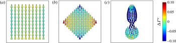
Moreover, specified square-like and diamond-like formations are also shown to be detrimental in terms of collective and individual effort (figure 10); nevertheless, their analysis is revealing of the hydrodynamic mechanisms at play in the ‘hourglass’ optimal solution. Indeed, although the fitness of the entire school is
 $f=0.004$
for both formations in figure 10(a,b), swimmers exposed on the left and right edges of the diamond formation suffer from high circulation expenditures, whereas those in the square formation generally do not. In the square formation, swimmers line up near the left and right edges of the school to help create greater net flow in the direction of travel. Conversely, swimmers at the front or rear of the diamond school benefit from schooling, whereas those in the square formation do not because of the counterflow produced from their immediate left and right neighbours. The optimal school shape solution of figure 10(c) takes advantage of these two effects: the ‘hourglass’ shape allows agents to line up near the boundary of the school and elongates in the travelling direction to reduce the counterflow from agents on the right and left edges.
Comparison between (a) the square formation (
 $f=0.004$
), (b) the diamond formation (
 $f=0.004$
) and (c) the optimal solution (
 $f_{\mathit{best}}=-0.067$
). The additional circulation change is computed for each swimmer and coloured accordingly. Simulations are run in the domain
 $[0,1]\times [0,1]$
with
 $\ell =5\times 10^{-4}$
,
 $v^{0}=5\ell$
,
 ${\it\rho}^{T}=10\ell$
,
 ${\it\delta}t=0.1$
,
 ${\it\varphi}=0.01$
,
 ${\it\gamma}=0.98$
and
 ${\it\epsilon}=0.01$
. The notation is as defined in § 2 and appendix A.

4. Discussion
We present a novel approach to studying schooling that involves coupling reinforcement learning and stochastic optimization with swimming agents (Tchieu et al. Reference Tchieu, Kanso and Newton2012) that explicitly account for hydrodynamic interactions. Swimmers are modelled as self-propelled finite-width dipoles and have the capability to adjust their speed and orientation to cope with varying hydrodynamic loads. The dipoles represent the far-field vortex wake of self-propelled natural swimmers, so that agents impart long-range velocity fields on all other agents via their dipolar strengths. These nonlinear hydrodynamic interactions critically affect schooling dynamics and individual swimming patterns. We show that classical agent models, which rely on a priori specified social rules, are not robust in the presence of hydrodynamics. In order to compensate for the hydrodynamics and to allow for schooling in the present agent-based model, we reverse-engineer the rules that are followed by the swimmers. This reverse engineering is achieved through a reinforcement learning algorithm that creates mappings between the dynamic environment of the agents and their actions so as to maximize a numerical reward. Our approach differs from the widely used handcrafted a priori behavioural rules, and allows us to examine how hydrodynamics affects swimmers’ decision-making in schooling. We find that adaptive swimming policies are crucial for maintaining schooling formations.
We evaluate the effectiveness of various formation patterns through an evolution strategy algorithm that identifies optimal schooling shapes and swimmer arrangements. We find that schools exhibiting minimal collective effort are ‘hourglass’-shaped and elongated in the swimming direction. Elongated shapes allow for drafting and pushing of swimmers arranged in internal striated patterns. Such internal striated patterns are found to be optimal independently of the overall shape of the school, which is qualitatively consistent with experimental observations (Misund et al. Reference Misund, Aglen and Fronaes1995; Parrish et al. Reference Parrish, Viscido and Grünbaum2002; Boschitsch et al. Reference Boschitsch, Dewey and Smits2014; Dewey et al. Reference Dewey, Quinn, Boschitsch and Smits2014).
Moreover, it is found that a tight packing of swimmers inside the school allows them to exploit flow-mediated interactions in terms of collective effort by enhancing the global dipolar field. At the same time, there is a limit to the amount of packing, as it becomes increasingly difficult for the swimmers to stay in formation due to stronger flow-mediated effects and increased probability of collisions. Such flow-mediated interactions can help to explain how certain fish travel in dense, elongated packs when migrating and foraging.
We remark that the present reverse-engineering approach to automatically identify interaction rules relative to a goal can be readily generalized to other forms of collective behaviour, from car traffic to social aggregations. In the context of schooling, future work is concerned with extending the use of these learning and optimization techniques to two- and three-dimensional viscous flows of multiple swimmers at intermediate Reynolds numbers (Gazzola, Hejazialhosseini & Koumoutsakos Reference Gazzola, Hejazialhosseini and Koumoutsakos2014). Reverse-engineering techniques, such as the ones proposed herein, can then be used to identify the various evolutionary traits that may have led to fish schooling.
Appendix A
A.1. Learning optimal behaviour in a fluid-mediated environment
A.1.1. Time integration and handling of collisions
The set of ODEs given in (2.2a,b
) is numerically integrated using the forward Euler method so as to retain flexibility in the decision selection process of the reinforcement learning algorithm. Since the equations become stiff as swimmers approach one another, the time step
 $\text{d}t$
is computed according to the minimum distance
 $d_{\mathit{min}}$
between all dipole swimmers present in the environment. We bound
 $\text{d}t$
with
 $\text{d}t=\text{d}t_{\mathit{max}}$
if
 $d_{\mathit{min}}\geqslant 2\ell$
and
 $\text{d}t=\text{d}t_{\mathit{min}}=5e^{-4}$
if
 $d_{\mathit{min}}\leqslant \ell /2$
. We require
 $\text{d}t_{\mathit{max}}$
to be dependent on the nominal velocity
 $v^{0}$
such that
 $\text{d}t_{\mathit{max}}=(5\ell C)/v^{0}$
. For the simulations here,
 $C=0.005$
.
Dipoles tend to collide if they are in close proximity with one another (Tchieu et al.
Reference Tchieu, Kanso and Newton2012). In a collision of two dipoles, both dipoles stop and annihilate their respective circulation strengths. We deal with this phenomenon by labelling colliding dipoles as ‘dead’ if
 $\text{d}t=\text{d}t_{\mathit{min}}$
. The dipoles’ circulations are artificially set to zero; hence dead dipoles no longer influence the other swimmers in the flow.
A.1.2. Error analysis of non-adaptive and adaptive schools of dipole swimmers
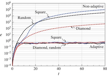
As observed in figure 6 of the main text and figure 11 here, in the presence of hydrodynamic interaction a given schooling arrangement is not maintained robustly without an adaptive dynamic response to the flow. We quantitatively demonstrate that schooling patterns can be maintained by swimmers through reinforcement learning. This is illustrated in figure 11, in which the errors (average distances to the target points,
 $e=\sum _{n}^{N}d_{n}/\ell$
) of the simulations in figure 6 are compared.
Time evolution of the sum of all errors between all agents and their respective assigned target points. The non-adaptive school simulations (dotted lines) of diamond (red), square (blue) and random (black) formations correspond to figure 6(b,e,h), respectively. The adaptive school simulations (bottom set of solid lines) of diamond (red), square (blue), and random (black) formations correspond to figure 6(c,f,i), respectively. The error is defined as
 $e=\sum _{n}^{N}d_{n}/\ell$
, i.e. the average distance to the target points.

A.2. Optimal schooling formations
We seek optimal schooling configurations by combining reinforcement learning with an evolutionary strategy. The algorithm of choice is the covariance matrix adaptation evolutionary strategy (CMA-ES) in its multihost, rank-
 ${\it\mu}$
and weighted recombination form (Hansen et al.
Reference Hansen, Muller and Koumoutsakos2003; Gazzola, Vasilyev & Koumoutsakos Reference Gazzola, Vasilyev and Koumoutsakos2011b
). The robustness of the CMA-ES is mainly controlled by the population size
 $p$
(Hansen et al.
Reference Hansen, Muller and Koumoutsakos2003). In this work, as a tradeoff between robustness and fast convergence, we set
 $p=100$
for all optimization computations. Bounds of the search space are enforced during the sampling through a rejection algorithm.
In this strategy, the CMA-ES determines the optimal configuration based on the metric of swimming effectiveness
 $f$
, while reinforcement learning determines the optimal policy for an agent to follow its target point under any configuration requested by the CMA-ES. Therefore, every cost function evaluation entails the CMA-ES dispatching a parameter set defining the geometry of the school, and then a reinforcement learning training period (
 ${\rm\Delta}T_{\mathit{training}}=10\,000$
) that allows the dipoles to learn how to swim in the given arrangement, followed by an evaluation interval (
 ${\rm\Delta}T_{\mathit{eval}}=100$
) in which the school effectiveness is measured and returned to the CMA-ES.
A.2.1. CMA-ES settings and parameterization for the optimization of school shape
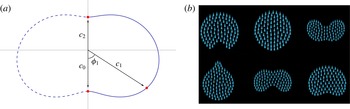
We evaluate how the overall school shape affects collective effort and optimize its effectiveness in terms of (2.7). To do so, we create a school by designing a general external shape and arranging the swimmers inside the boundary by placing them maximally distant from one another and the boundary. The shape of the school is dictated by a cubic spline-based parameterization introduced in Rossinelli, Chatagny & Koumoutsakos (Reference Rossinelli, Chatagny and Koumoutsakos2011). According to this parameterization, the external school shape is represented as
 $c=S({\it\phi})$
, where
 $c$
is the radial distance from the origin in the polar plane,
 ${\it\phi}\in [0,{\rm\pi}]$
is the angle and
 $S$
is the piecewise polynomial of the cubic spline. The spline control points (red dots in figure 12), expressed in polar coordinates, are
 $(c_{0},0)$
,
 $(c_{1},{\it\phi}_{1})$
and
 $(c_{2},0)$
, with the radii defined as
 $c_{1}=k_{1}\cdot c_{0}$
and
 $c_{2}=k_{2}\cdot b_{0}$
where
 $k_{1}$
and
 $k_{2}$
are constants. The school shape is completed by reflecting the obtained spline profile. Unlike Rossinelli et al. (Reference Rossinelli, Chatagny and Koumoutsakos2011), the area of the school shape
 $A(S)$
, and therefore
 $c_{0}$
, is controlled via an extra parameter, namely the average distance
 $d_{\mathit{avg}}$
between swimmers, such that
 $b_{0}:A(S)=N\cdot d_{\mathit{avg}}^{2}$
, where
 $N$
is the number of dipoles. Therefore, the shape of the school depends on the four parameters
 $\boldsymbol{p}=\{d_{\mathit{avg}},k_{1},k_{2},{\it\phi}_{1}\}$
. These free parameters are varied within the search space
 $[1,5]\times [0.1,2]\times [0.1,2]\times [{\rm\pi}/6,5{\rm\pi}/6]\in \mathbb{R}^{4}$
during the optimization.
Parameterization of the shape of the school and a representative subset of candidate solutions. The parameterization generates the solid line (blue) and is reflected to create the symmetric complement (dashed line). The control points are depicted as red dots.

A.2.2. CMA-ES settings for the optimization of the internal lattice structure of a school
The free parameters
 $h,b$
and
 ${\it\beta}$
for the diamond, rectangular and hexagonal search space (see figure 8
a–c) are varied in the ranges
 $[0,50\ell ]\times [0,50\ell ]\times [0,{\rm\pi}/2]\in \mathbb{R}^{3}$
,
 $[0,50\ell ]\times [0,50\ell ]\times [0,{\rm\pi}/2]\in \mathbb{R}^{3}$
and
 $[0,50\ell ]\times [0,{\rm\pi}/6]\in \mathbb{R}^{2}$
, respectively, during the optimization.