

Introduction
Anthropogenic activities, particularly the emission of greenhouse gases, have significantly increased the average global surface temperature (Harley et al., Reference Harley, Anderson, Demes, Jorve, Kordas and Coyle2012). Between 2011 and 2020, global mean surface temperatures were 1.1°C above 1850–1900 levels (IPCC, Reference Lee and Romero2023). This warming trend has not only altered precipitation patterns but has also resulted in notable shifts in ecosystems and species distribution ranges, and the timing of seasonal events (Büntgen et al., Reference Büntgen, Piermattei, Krusic, Esper, Sparks and Crivellaro2022; Esperon-Rodriguez et al., Reference Esperon-Rodriguez, Tjoelker, Lenoir, Baumgartner, Beaumont and Nipperess2022; Stemkovski et al., Reference Stemkovski, Bell, Ellwood, Inouye, Kobori and Lee2023). These changes form part of the multifaceted array of stressors induced by climate change, which involves alterations in temperature, heightened atmospheric CO2 levels, and more frequent and intense occurrences of droughts and extreme water flow events. The vulnerability of ecosystems and their inhabitants to climate change varies globally, with sub-Saharan Africa being disproportionately affected (Kompas et al., Reference Kompas, Pham and Che2018; Sintayehu, Reference Sintayehu2018; Affoh et al., Reference Affoh, Zheng, Dangui and Dissani2022; IPCC, Reference Lee and Romero2023).
Freshwater ecosystems are among the most threatened ecosystems and vulnerable to climate change (Collen et al., Reference Collen, Whitton, Dyer, Baillie, Cumberlidge and Darwall2014; Hannah, Reference Hannah2021; Singh et al., Reference Singh, Singh, Singh, Mishra, Thokchom, Qiu, Singh and Iyer2021; Vári et al., Reference Vári, Podschun, Erős, Hein, Pataki and Iojă2022; Sayer et al., Reference Sayer, Fernando, Jimenez, Macfarlane, Rapacciuolo and Böhm2025). They cover < 0.8% of the Earth’s surface and serve as habitats for c. 10% of all known vertebrate species and 2% of all known invertebrate species. Freshwater ecosystems deliver vital services to both people and ecosystems (Desta et al., Reference Desta, Lemma and Fetene2012). Globally, primary freshwater crabs are a species-rich assemblage of macro-invertebrates characterized by high levels of diversity and endemism (Cumberlidge & Daniels, Reference Cumberlidge and Daniels2022). Freshwater crabs undergo direct development, lacking a dispersive larval stage, and complete their entire life cycle in freshwater (Cumberlidge et al., Reference Cumberlidge, Peter, Yeo, Magalhães, Campos and Alvarez2009). They are crucial to freshwater systems as they play a significant role in nutrient cycling and maintaining ecosystem dynamics (Yeo et al., Reference Yeo, Ng, Cumberlidge, Magalhães, Daniels, Campos, Balian, Lévequè, Segers and Martens2008; Cumberlidge et al., Reference Cumberlidge, Peter, Yeo, Magalhães, Campos and Alvarez2009). A comprehensive global review of the threats and conservation status of primary freshwater crabs indicated that approximately one-sixth of all species are at risk of extinction (Cumberlidge et al., Reference Cumberlidge, Peter, Yeo, Magalhães, Campos and Alvarez2009).
South Africa’s freshwater ecosystems face significant direct threats from climate change and climate-related factors that will affect freshwater species populations (Mitchell, Reference Mitchell2013; Job et al., Reference Job, Skowno and Currie2025; van Deventer et al., Reference Van Deventer and Nel2025). Projections indicate that rainfall patterns will shift, with some regions experiencing increased precipitation and others facing declines, along with heightened severity of extreme events (IPCC, 2017; Davis-Reddy & Vincent, Reference Davis-Reddy and Vincent2017). These changes are expected to exacerbate flooding, fragment habitats, change water flow regimes and facilitate the spread of invasive freshwater species (IPCC, 2017). To aid our understanding of the future impact of climate change on southern African freshwater crabs, we use species distribution models (Guisan et al., Reference Guisan, Thuiller and Zimmermann2017; Zhang et al., Reference Zhang, Xu, Capinha, Weterings and Gao2019; Yousefi et al., Reference Yousefi, Jouladeh-Roudbar and Kafash2020; Jinga & Manyangadze, Reference Jinga and Manyangadze2024). These models have been used to forecast species distributions and identify climatic refugia (Ashrafzadeh et al., Reference Ashrafzadeh, Naghipour, Haidarian, Kusza and Pilliod2019; Sheykhi Ilanloo et al., Reference Sheykhi Ilanloo, Khani, Kafash, Valizadegan, Ashrafi and Loercher2021; Sierra-Morales et al., Reference Sierra-Morales, Rojas-Soto, Ríos-Muñoz, Ochoa-Ochoa, Flores-Rodríguez and Almazán-Núñez2021; Vaissi, Reference Vaissi2021), and to examine changes in species distribution, richness and composition as a result of climate change-induced alterations (Kwon et al., Reference Kwon, Bae, Hwang, Kim and Park2015; Zhang et al., Reference Zhang, Xu, Capinha, Weterings and Gao2019; Prieto-Torres et al., Reference Prieto-Torres, Lira-Noriega and Navarro-Sigüenza2020; Yousefi et al., Reference Yousefi, Jouladeh-Roudbar and Kafash2020). Additionally, species distribution models have proven useful in refining distributions and identifying high-priority areas for conservation (Cuesta et al., Reference Cuesta, Peralvo, Merino-Viteri, Bustamante, Baquero and Freile2017; Moradi et al., Reference Moradi, Ilanloo, Kafash and Yousefi2019; Hameed et al., Reference Hameed, Din, Ali, Kabir, Younas and Rehman2020; Ramírez-Albores et al., Reference Ramírez-Albores, Prieto-Torres, Gordillo-Martínez, Sánchez-Ramos and Navarro-Sigüenza2021; Kafash et al., Reference Kafash, Ashrafi and Yousefi2022).
We hypothesize, given the predicted impact of climate change, that South African freshwater crab (Potamonautes) distributions and suitable habitat will change in response to a changing climate, with some species undergoing range contractions and others range expansion. To investigate these predicted changes, we use ecological niche modelling to identify potential unexplored habitats for 17 Potamonautes freshwater crab species. Additionally, we aim to assess the future effectiveness of current protected areas in South Africa in safeguarding Potamonautes species by evaluating their projected distributions, current IUCN Red List status and potential future conservation status. Noticeably, none of the current freshwater conservation management plans in South Africa were specifically developed to include freshwater crabs or any co-occurring freshwater species. We expect that not all species will have similar responses to climate change and that the current protected area network may not protect all species sufficiently.
Methods
Occurrence data
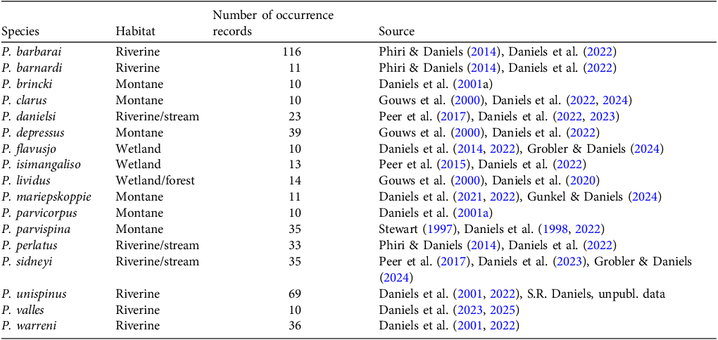
Occurrence data for 17 Potamonautes freshwater crab species were collected from previous studies and curated through the Red Listing process for the species; they include specimen records, unpublished data and iNaturalist observations that were verified by author SRD and used in Daniels et al. (Reference Daniels, Barnes, Peer, Egan, Taylor, Taylor and Van Der Colff2022) (Table 1, Fig. 1). This included species for which ≥10 records are known, and all are categorized on the IUCN Red List as Least Concern. Three additional, recently described, point-endemic species (P. mhlope, P. ngoyensis and P. ntendekaensis) are categorized as Vulnerable but there are insufficient records for these three species to model their projected future distribution under climatic models. In data validation and curation we only included records ≥ 1 km apart, as the climatic variables employed have a spatial resolution of 1 km. The spatial data were obtained on 20 September 2024 from the South African Red List (D. van der Colff, unpubl. data).
The 17 Potamonautes species for which we modelled present and future distribution, with number of occurrence records and data sources.

Table 1 Long description
A table with 17 rows and 4 columns. The columns are labeled Species, Habitat, Number of occurrence records, and Source. The table lists different Potamonautes species, their habitats, the number of occurrence records for each species, and the sources of the data. Each row provides specific details for a species, including whether it is riverine, montane, or wetland, and the corresponding number of records. The sources include various studies and publications.
Climatic variables
We used all 19 bioclimatic variables from WorldClim2 (Fick & Hijmans, Reference Fick and Hijmans2017), at a resolution of 30 arc-seconds (c. 1 km2), selecting only those with low collinearity (i.e. with variance inflation factor < 5), to model freshwater crab species distribution under present and future climatic conditions (Supplementary Table 1). To consider uncertainty in climate model projections, we used two general circulation models: CMCC-ESM2 and GISS-E2-1G (Sanderson et al., Reference Sanderson, Knutti and Caldwell2015) for 2081–2100 under the Coupled Model Intercomparison Project Phase 6 (CMIP6) modelling framework. These models were chosen for their general effectiveness and ease of use (Sanderson et al., Reference Sanderson, Knutti and Caldwell2015). The 2081–2100 time frame was selected to align with the United Nations Framework Convention on Climate Change Paris Agreement’s (2015) long-term mitigation goals, which extend to the end of the century and beyond.
Climatic niche comparison
The potential distributions of all 17 Potamonautes species were extrapolated statistically. Climatic data were extracted for the locality of each record using the Raster package (Hijmans, Reference Hijmans2022) in R 4.4.2 (R Core Team, 2025), with duplicate or nearby localities that shared the same raster cell removed using the spThin package in R (Aiello-Lammens et al., Reference Aiello-Lammens, Boria, Radosavljevic, Vilela and Anderson2015). All variables were standardized in MaxEnt 3.4.4 (Phillips et al., Reference Phillips, Anderson, Dudík, Schapire and Blair2017) and the bioclimatic variables for each population were subjected to a principal component analysis, using the R function pcrcomp. A permutational multivariate analysis of variance with 9,999 permutations was used to examine differences in climate between the locations of the species’ populations, using the R package vegan (Oksanen et al., Reference Oksanen, Simpson, Blanchet, Kindt, Legendre and Minchin2022).
Climatic niche modelling
Information obtained from the climatic niche comparison was used to visualize the ecological niche of the 17 Potamonautes species (Fig. 1). Correlated variables (with a Pearson’s correlation coefficient > 0.7) for the 19 bioclimatic variables were calculated, and assessed using the R package CorrPlot (Wei & Simko, Reference Wei and Simko2021). Additionally, the R package usdm (Naimi et al., Reference Naimi, Hamm, Groen, Skidmore and Toxopeus2014) was used to conduct a variance inflation factor analysis for the independent variables using a threshold of five, with the remaining limiting climatic variables used to generate the models. A custom R script was used to specify a fixed distance radius of 200 km based on the occurrence records for model building to correct the models for overprediction, and to produce minimum convex polygons of the distribution for each taxon. The R package ENMeval 2.0 (Kass et al., Reference Kass, Muscarella, Galante, Bohl, Pinilla-Buitrago and Boria2021) was used to determine the optimum feature class and regularization multiplier for model construction and to convert the continuous probability surfaces to binary models representing either suitable or unsuitable climatic conditions based on the maximum test specificity and sensitivity thresholds.
Summary of data preparation for species habitat suitability maps of Potamonautes species in South Africa: (a) preparing occurrence records of the 17 species by collating and validating records, (b) generating niche models to examine the species’ environmental tolerances, and using MaxEnt modelling to generate species distribution models based on environmental variables, (c) using the species habitat suitability models to model species distribution under two future climate scenarios, (d) intersecting maps of present species ranges with the protected area network, and (e) intersecting future species ranges under two climate scenarios with the protected area network. (Readers of the printed journal are referred to the online article for colour versions of the figures.)

Species distribution modelling
The niche modelling results were used to develop maximum entropy (MaxEnt) models (Phillips et al., Reference Phillips, Anderson, Dudík, Schapire and Blair2017) to predict the current and future distribution of the 17 Potamonautes species. Models were calibrated using the compiled occurrence data (Table 1, Fig. 1). The area under the receiver operating characteristic curve (AUC) was used to evaluate the predictive performance of the models. Values range from 0 to 1, with a value of 0.5 indicating that the performance of the model is not better than random, and values close to 1.0 indicating good model performance.
Protected area coverage
To determine the representation of present and future suitable habitat for the 17 Potamonautes species in the South African protected area network, the species distribution models were overlaid on the protected areas layer. The models were converted to binary suitable–unsuitable maps through use of the 10 percentile training presence logistic threshold (Vale et al., Reference Vale, Souza, Alves and Crouzeilles2018). Then, the area of current and future suitable habitats within protected areas was calculated for each species using the raster package in R (Hijmans, Reference Hijmans2017). Protected area layers were obtained from SANBI (2026).
Bioclimatic variable assessment
To determine the importance of each bioclimatic variable for the 17 Potamonautes species, suitable habitat modelling was derived by scaling the mean contribution of each bioclimatic variable based on species representation, with a penalty applied to variables used by < 3 species (Yousefi et al., Reference Yousefi, Naderloo and Keikhosravi2022). The score has the range 0–100, with higher scores indicating a higher level of importance for that variable in the species distribution models.
 $\eqalign {Adjusted\;composite\;score & = Mean\;contribution \cr & \times \left( {{{Number\;of\;species} \over {Max.\;species}}} \right) \cr & \times Penalty\;factor}$
Mean contribution is the average contribution of a specific bioclimatic variable across all species that show some response to it; it quantifies how influential that variable is in determining a species’ suitable habitat, with a higher mean contribution suggesting the variable plays a greater role in the ecological or biological processes under study. The mean contribution is based on the mean contribution of each bioclimatic variable based on species representation, with a penalty applied to variables used by < 3 species. Number of species is the number of species that use the given bioclimatic variable; it provides insight into how relevant the variable is for the species in the dataset. Max. species is the maximum number of species that use any single bioclimatic variable within the dataset; it is crucial for normalization, as it allows the adjusted composite score to account for the relative importance of each variable in relation to the most widely used variable. Penalty factor is a corrective factor (0.5) applied to account for scenarios where a bioclimatic variable is used by fewer species than a predefined threshold (< 3 species in this case); if the number of species is below this threshold, it may indicate the variable is less relevant in ecological modelling, and it reduces the adjusted composite score proportionally, thereby emphasizing the importance of variables that are applicable to a wider range of species.
Results
Climate change models
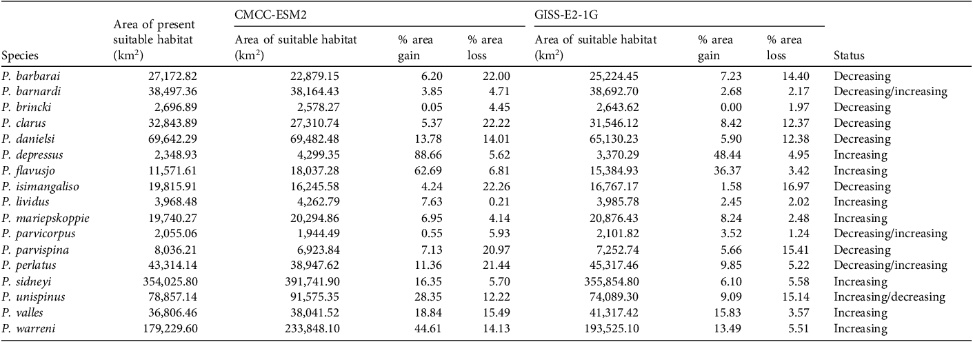
Our findings indicate that each species is predicted to experience both gains and losses in suitable habitat under the different general circulation models (Figs 2–3). For illustration, we selected two freshwater crab species. For P. isimangaliso we observed a reduction in suitable habitat and in protected area coverage under future climatic scenarios (Fig. 2) and, conversely, we observed habitat gain for P. flavusjo (Fig. 3). Projections for all species are presented in Supplementary Figs 1–4. However, some species have greater habitat losses than gains, resulting in a net loss of suitable area, and others will gain more than they lose, leading to an overall net increase in suitable habitat. Six species (P. barbarai, P. brincki, P. clarus, P. danielsi, P. isimangaliso, P. parvispina), including at least three mountain dwelling species (P. brincki, P. clarus, P. parvispina), are predicted to experience a net loss of suitable area under both the CMCC-ESM2 and GISS-E2-1G models. Seven species (P. depressus, P. flavusjo, P. lividus, P. mariepskoppie, P. sidneyi, P. valles, P. warreni) are predicted to experience a net gain of suitable area under both general circulation models. Four, mainly riverine species (P. barnardi, P. parvicorpus P. perlatus, P. unispinus), are predicted to experience either a decrease or increase in suitable habitat depending on the general circulation model (Table 2).
Potamonautes isimangaliso, showing (a) the approximate area of its present distribution, (b) its predicted future distribution under climatic scenarios CMCC-ESM2 CMIP6 and GISS-E2-1G CMIP6, and predicted future areas of persistence, loss and expansion under (c) CMCC-ESM2 CMIP6 and (d) GISS-E2-1G CMIP6.

Fig. 2 Long description
Panel A: A map of South Africa highlighting the present distribution area of Potamonautes isimangaliso. Panel B: A map showing the predicted future distribution of Potamonautes isimangaliso under two climate scenarios, CMCC-ESM2 CMIP6 and GISS-E2-1G CMIP6, with areas of future distribution marked in different colors. Panel C: A map illustrating the predicted future areas of persistence, loss, and expansion of Potamonautes isimangaliso under the CMCC-ESM2 CMIP6 scenario. Panel D: A map showing the predicted future areas of persistence, loss, and expansion of Potamonautes isimangaliso under the GISS-E2-1G CMIP6 scenario.
Potamonautes flavusjo, showing (a) the approximate area of its present distribution, (b) its predicted future distribution under climatic scenarios CMCC-ESM2 CMIP6 and GISS-E2-1G CMIP6, and predicted future areas of persistence, loss and expansion under (c) CMCC-ESM2 CMIP6 and (d) GISS-E2-1G CMIP6.

Species distribution modelling results for all 17 Potamonautes species for present and future climate scenarios (CMCC-ESM2 CMIP6 and GISS-E2-1G CMIP6).

Table 2 Long description
The table presents data on the area of suitable habitat for 17 Potamonautes species under two climate models, CMCC-ESM2 and GISS-E2-1G. It includes columns for the area of present suitable habitat, area of suitable habitat under each model, percentage area gain, percentage area loss, and the status of each species. Row 1: P. barbarai, 27,172.82, 22,879.15, 6.20, 22.00, 25,224.45, 7.23, 14.40, Decreasing. Row 2: P. barnardi, 38,497.36, 38,164.43, 3.85, 4.71, 38,692.70, 2.68, 2.17, Decreasing/increasing. Row 3: P. brincki, 2696.89, 2578.27, 0.05, 4.45, 2643.62, 0.00, 1.97, Decreasing. Row 4: P. clarus, 32,843.89, 27,310.74, 5.37, 22.22, 31,546.12, 8.42, 12.37, Decreasing. Row 5: P. danielsi, 69,642.29, 69,482.48, 13.78, 14.01, 65,130.23, 5.90, 12.38, Decreasing. Row 6: P. depressus, 2348.93, 4299.35, 88.66, 5.62, 3370.29, 48.44, 4.95, Increasing. Row 7: P. flavusjo, 11,571.61, 18,037.28, 62.69, 6.81, 15,384.93, 36.37, 3.42, Increasing. Row 8: P. isimangaliso, 19,815.91, 16,245.58, 4.24, 22.26, 16,767.17, 1.58, 16.97, Decreasing. Row 9: P. lividus, 3968.48, 4262.79, 7.63, 0.21, 3985.78, 2.45, 2.02, Increasing. Row 10: P. mariepskoppie, 19,740.27, 20,294.86, 6.95, 4.14, 20,876.43, 8.24, 2.48, Increasing. Row 11: P. parvicorpus, 2055.06, 1944.49, 0.55, 5.93, 2101.82, 3.52, 1.24, Decreasing/increasing. Row 12: P. parvispina, 8036.21, 6923.84, 7.13, 20.97, 7252.74, 5.66, 15.41, Decreasing. Row 13: P. perlatus, 43,314.14, 38,947.62, 11.36, 21.44, 45,317.46, 9.85, 5.22, Decreasing/increasing. Row 14: P. sidneyi, 354,025.80, 391,741.90, 16.35, 5.70, 355,854.60, 6.10, 5.58, Increasing. Row 15: P. unispinus, 78,857.14, 91,575.35, 28.35, 12.22, 74,089.30, 9.09, 15.14, Increasing/decreasing. Row 16: P. valles, 36,806.46, 38,041.52, 18.84, 15.49, 41,317.42, 15.83, 3.57, Increasing. Row 17: P. warreni, 179,229.60, 233,848.10, 44.61, 14.13, 193,525.10, 13.49, 5.51, Increasing.
Protected area coverage under present and future climates
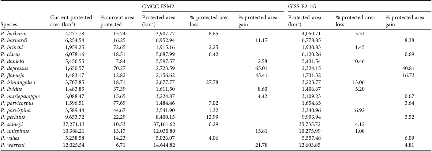
An average of 27.95% (6776.67 km2) of present suitable habitat is protected for all species. Depending on the climate change scenario (CMCC-ESM2 or GISS-E2-1G), some species are projected to be more at risk than others of losing currently protected area. The five species that are projected to lose the most suitable, protected area under the CMCC-ESM2 scenario are P. isimangaliso, P. perlatus, P. barbarai, P. parvicorpus and P. clarus. The five species that are projected to lose the most suitable, protected area under the GISS-E2-1G scenario are P. isimangaliso, P. parvispina, P. barbarai, P. lividus and P. sidneyi. The five species that are projected to gain the most suitable, protected area under the CMCC-ESM2 model are P. depressus, P. flavusjo, P. warreni, P. unispinus and P. barnardi. The five species that are projected to gain the most suitable, protected area under the GISS-E2-1G model are P. depressus, P. flavusjo, P. barnardi, P. valles and P. warreni (Table 3).
Area of protected suitable habitat (km2) for the 17 Potamonautes species under current climate and future climate scenarios (CMCC-ESM2 CMIP6 and GISS-E2-1G CMIP6).

Table 3 Long description
A table comparing protected areas for various species under different climate scenarios. The table has 17 rows and 12 columns. Column headers are Species, Current protected area (km2), % current area protected, Protected area (km2) under CMCC-ESM2, % protected area loss under CMCC-ESM2, % protected area gain under CMCC-ESM2, Protected area (km2) under GISS-E2-1G, % protected area loss under GISS-E2-1G, and % protected area gain under GISS-E2-1G. Row labels are species names. Row 1: P. barbarai, 4277.78, 15.74, 3907.77, 8.65, 6778.85, 4050.71, 5.31, 8.38. Row 2: P. barnardi, 6254.54, 16.25, 6952.94, 11.17, 6778.85, 4050.71, 5.31, 8.38. Row 3: P. brincki, 1959.25, 72.65, 1915.16, 2.25, 1930.83, 1406.67, 1.45, 6.12. Row 4: P. clarus, 6078.16, 18.51, 5687.99, 6.42, 6120.26, 5431.54, 0.46, 0.69. Row 5: P. danielsi, 5456.55, 7.84, 5597.57, 2.58, 5431.54, 0.46, 0.69. Row 6: P. depressus, 1650.57, 70.27, 2723.59, 65.01, 2324.15, 1673.12, 40.81, 16.73. Row 7: P. flavusjo, 1483.17, 12.82, 2156.62, 45.41, 1731.32, 3223.77, 13.06, 16.73. Row 8: P. isimangaliso, 3707.85, 18.71, 2677.77, 27.78, 3223.77, 13.06, 1406.67, 5.20. Row 9: P. lividus, 1483.85, 37.39, 1611.50, 8.60, 1406.67, 5.20, 3109.23, 4.42. Row 10: P. mariepskoppie, 3088.47, 15.65, 3224.87, 4.42, 3109.23, 4.42, 3109.23, 4.42. Row 11: P. parvicorpus, 1596.51, 77.69, 1484.46, 7.02, 1654.65, 3.64, 3340.96, 6.92. Row 12: P. parvispina, 3589.44, 44.67, 3541.90, 1.32, 3340.96, 6.92, 9993.94, 3.52. Row 13: P. perlatus, 9653.72, 22.29, 8400.15, 12.99, 9993.94, 3.52, 9993.94, 3.52. Row 14: P. sidneyi, 37271.13, 10.53, 37161.62, 0.29, 35735.72, 4.12, 5557.48, 6.09. Row 15: P. unispinus, 10388.21, 13.17, 12030.80, 15.81, 10275.99, 1.08, 12603.85, 4.81. Row 16: P. valles, 5238.51, 14.23, 5026.07, 4.06, 5557.48, 6.09, 12603.85, 4.81. Row 17: P. warreni, 12025.54, 6.71, 14644.82, 21.78, 12603.85, 4.81.
Variable importance for freshwater crabs
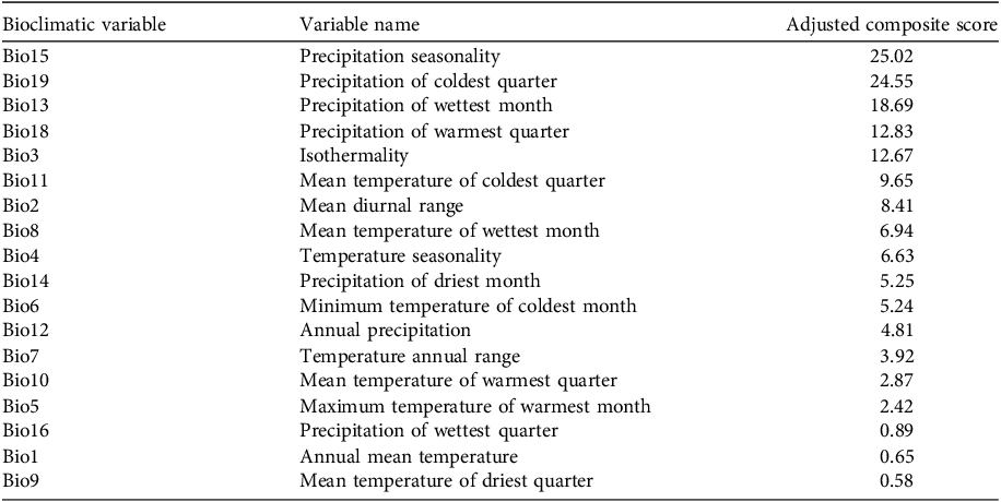
Estimating variable importance with the adjusted composite score indicates that precipitation plays an important role in shaping species’ suitable habitat, especially when precipitation has a seasonal aspect. The most important variables are precipitation seasonality (adjusted composite score 25.02), precipitation of the coldest quarter (24.55) and precipitation of the wettest month (18.69; Table 4).
Adjusted composite score for each bioclimatic variable, ordered from high to low. Higher scores indicate greater importance in the species distribution modelling. Bio 17 contributed little to the species distribution model and was excluded.

Table 4 Long description
The table presents bioclimatic variables, their variable names, and adjusted composite scores. It has three columns: Bioclimatic variable, Variable name, and Adjusted composite score. The table lists 19 rows of data. Row 1: Bio15, Precipitation seasonality, 25.02. Row 2: Bio19, Precipitation of coldest quarter, 24.55. Row 3: Bio13, Precipitation of wettest month, 18.69. Row 4: Bio18, Precipitation of warmest quarter, 12.83. Row 5: Bio3, Isothermality, 12.67. Row 6: Bio11, Mean temperature of coldest quarter, 9.65. Row 7: Bio2, Mean diurnal range, 8.41. Row 8: Bio8, Mean temperature of wettest month, 6.94. Row 9: Bio4, Temperature seasonality, 6.63. Row 10: Bio14, Precipitation of driest month, 5.25. Row 11: Bio6, Minimum temperature of coldest month, 5.24. Row 12: Bio12, Annual precipitation, 4.81. Row 13: Bio7, Temperature annual range, 3.92. Row 14: Bio10, Mean temperature of warmest quarter, 2.87. Row 15: Bio5, Maximum temperature of warmest month, 2.42. Row 16: Bio16, Precipitation of wettest quarter, 0.89. Row 17: Bio1, Annual mean temperature, 0.65. Row 18: Bio9, Mean temperature of driest quarter, 0.58.
Discussion
Our hypothesis that the future distributions of freshwater crabs will be affected by climate change was corroborated. The species distribution models indicate that predicted climate change could drive substantial shifts in habitat suitability, with some species predicted to gain habitat and others to lose considerable areas of habitat. Other studies, such as of the Eurasian freshwater crab genus Potamon (Muths et al., Reference Muths, Chambert, Schmidt, Miller, Hossack and Jol2017; Wen et al., Reference Wen, Wu, Cheng, Chang, Yang and Xia2017; Kafash et al., Reference Kafash, Ashrafi, Ohler, Yousefi, Malakoutikhah and Koehler2018; Yousefi et al., Reference Yousefi, Naderloo and Keikhosravi2022) have also demonstrated that species responses to climate change can vary even among closely related taxa. Additionally, we found that some species are projected to experience a reduction in protected habitat, and others may benefit from increases, although patterns vary. Precipitation variables, principally precipitation seasonality, precipitation of the coldest quarter and precipitation of the wettest month, have the greatest effects on future species distributions. Similarly, precipitation has also been demonstrated to be important in the distribution of other aquatic taxa such as amphibians and fishes (Courtois et al., Reference Courtois, Michel, Martinez, Dewynter, Ficotola and Fouquet2016; Clavergo et al., Reference Clavero, Calzada, Esquivias, Verissimo, Hermoso and Qninb2018; Kajee et al., Reference Kajee, Henry, Dallas, Griffiths, Peff and Van Der Colff.2023).
Despite its utility, the MaxEnt modelling approach has known limitations, particularly its sensitivity to sample bias and overfitting, especially when applied to small or biased datasets (Phillips et al., Reference Phillips, Anderson, Dudík, Schapire and Blair2017). An example of this limitation is illustrated by P. sidneyi. The distribution map (Supplementary Fig. 3) suggests that P. sidneyi has a predominantly eastern distribution, but it occurs over a broader area, including near Upington in the Northern Cape Province. This record was included in the modelling dataset, yet the predominance of data points in the eastern regions caused the model to exclude the Northern Cape, leading to an incomplete prediction of distribution. There are also other inherent limitations in ecological modelling. These challenges highlight the complexities of using species distribution models in ecological research and the need for careful consideration of methodological limitations.
Using two CMIP6 climate models (CMCC-ESM2 and GISS-E2-1G), we found that climate change is likely to drive species-specific shifts in habitat suitability. Although some species are projected to experience habitat expansion, others face substantial reductions in both suitable habitat and protected area coverage, suggesting heightened vulnerability to climate change. For P. isimangaliso these projected declines indicate the potential need to reassess its IUCN Red List status, as the species may face an elevated risk of extinction under future climate conditions. Given the considerable contraction in habitat, the species will probably need to be recategorized as Vulnerable, based on a highly restricted range. Precipitation-related variables were the primary predictors of Potamonautes distributions, and this reliance on precipitation-driven environments, combined with limited dispersal abilities, underscores the sensitivity of freshwater crabs to changes in seasonal water availability. These findings highlight potential disruptions to ecological stability as these patterns shift.
Analysis of protected areas indicates that different global circulation models may project different outcomes for individual Potamonautes species. Despite these differences, both scenarios consistently project habitat losses for P. barbarai and P. isimangaliso, with P. isimangaliso being particularly vulnerable because of its below-average protected area coverage (< 27.95%) and the highest projected loss of protected habitat (27.78% under CMCC-ESM2 and 13.06% under GISS-E2-1G). Coupled with a marked reduction in overall suitable habitat (Table 2), P. isimangaliso appears to be the South African freshwater crab species most at risk under future climate change.
Conversely, several species are expected to experience gains in protected habitat, potentially benefiting from climate-induced range shifts. Potamonautes depressus and P. flavusjo appear to be the least vulnerable species under future climate conditions, with protected habitat increases of 65.01% and 45.41%, respectively, under CMCC-ESM2 and 40.81% and 16.73%, respectively, under GISS-E2-1G. These projections suggest that climate-driven range shifts into the existing protected area network may help buffer these species against adverse climate impacts.
Species projected to lose suitable habitat have three potential responses: adaptation to new climatic conditions, movement to higher elevations where conditions are more favourable, or potential extinction (Yousefi et al., Reference Yousefi, Jouladeh-Roudbar and Kafash2020). Of the six species facing habitat loss, three are mountain dwellers (P. brincki, P. clarus, P. parvispina) and could ultimately reach an elevation threshold beyond which suitable habitat is unavailable, restricting their capacity to adapt (Elsen & Tingley, Reference Elsen and Tingley2015; Freeman et al., Reference Freeman, Song, Feeley and Zhu2021). Similarly, riverine species such as P. barbarai and P. danielsi may face comparable constraints as their viable habitats diminish as a consequence of rise in sea levels, and the intrusion of sea water into freshwater habitats.
Potamonautes isimangaliso appears to be particularly vulnerable to climate change as it is the only semi-terrestrial burrowing species expected to lose substantial suitable habitat under both global circulation model scenarios. It is a narrow endemic that inhabits highly fragmented ephemeral pans in coastal north-eastern KwaZulu-Natal (Fig. 2). The limited population connectivity of the species potentially limits recolonization events, although the dispersal capacity of the species is unknown. Unlike riverine species, this semi-terrestrial burrowing crab is unlikely to have the physiological capabilities to shift to higher elevations through stream usage. Additionally, CMIP6 projections for South Africa indicate declining precipitation alongside more extreme weather events, including intense rainfall and flooding, which could further fragment habitats by reducing the ephemeral water bodies that support P. isimangaliso (Almazroui et al., Reference Almazroui, Saeed, Saeed, Nazrul Islam, Ismail and Klutse2020; Karypidou et al., Reference Karypidou, Katragkou and Sobolowski2022; Bobde et al., Reference Bobde, Akinsanola, Folorunsho, Adebiyi and Adeyeri2024). The peripheral populations of P. isimangaliso outside the iSimangaliso Wetland Park are particularly vulnerable to localized extinctions as a result of encroaching human settlements. The projected increases in both suitable habitat and protected area coverage for P. depressus, P. flavusjo, and P. warreni suggest resilience to climate change. Semi-terrestrial species such as P. flavusjo may benefit from fragmented habitats and variable rainfall, as increased flooding events offer occasional dispersal opportunities across isolated areas (Grobler & Daniels, Reference Grobler and Daniels2024).
In summary, our findings highlight the need for conservation strategies tailored to each species’ expected unique response to climate change, emphasizing the importance of habitat connectivity and protected areas in supporting resilience (Muths et al., Reference Muths, Chambert, Schmidt, Miller, Hossack and Jol2017; Wen et al., Reference Wen, Wu, Cheng, Chang, Yang and Xia2017; Hannah, Reference Hannah2021; Yousefi et al., Reference Yousefi, Naderloo and Keikhosravi2022). Although protected areas serve as essential tools for global biodiversity conservation (Geldmann et al., Reference Geldmann, Barnes, Coad, Craigie, Hockings and Burgess2013; Gray et al., Reference Gray, Hill, Newbold, Hudson, Börger and Contu2016), they have been established based on present-day biodiversity distributions. Climate change poses a challenge to their effectiveness by altering species distributions (Johnston et al., Reference Johnston, Ausden, Dodd, Bradbury, Chamberlain and Jiguet2013; Hoffmann et al., Reference Hoffmann, Irl and Beierkuhnlein2019; Hannah, Reference Hannah2021). In this context, species distribution models are valuable for evaluating the effectiveness of protected areas in conserving biodiversity under changing environmental conditions (Berteaux et al., Reference Berteaux, Ricard, St-Laurent, Casajus, Perie and Beauregard2018; Hoveka et al., Reference Hoveka, Van Der Bank and Davies2020; Petersen et al., Reference Petersen, Savini, Gray, Baker-Whatton, Bis and Chutipong2021).
The adjusted composite score emphasizes the critical role of precipitation, and especially precipitation seasonality, in predicting freshwater crab species distributions, both current and future, as also found elsewhere (Yousefi et al., Reference Yousefi, Naderloo and Keikhosravi2022). Most freshwater crabs have limited dispersal abilities, relying on access to water for oxygen absorption and nitrogen excretion. Consequently, their movement is restricted to short land bridges in high-humidity regions or to rainy seasons in areas with marked seasonality.
Globally, at least one-sixth of freshwater decapods are threatened, but 28% of species are threatened in the Afrotopical region (Cumberlidge et al., Reference Cumberlidge, Peter, Yeo, Magalhães, Campos and Alvarez2009). A recent study suggested that 25% of the global freshwater fauna are threatened with extinction (Sayer et al., Reference Sayer, Fernando, Jimenez, Macfarlane, Rapacciuolo and Böhm2025). Conservation efforts for freshwater crabs will need to prioritize habitat connectivity and the identification of potential climate refugia, to support species persistence. Our study provides the first exploration of these interactions and insights to guide management and policy decisions for Potamonautes species at risk. We recommend the development of an integrated conservation management plan that includes additional aquatic groups, with their distributions also modelled under future climatic scenarios, and of monitoring programmes for threatened freshwater macro-invertebrates (although appropriate funding in developing countries such as South Africa is a major challenge).
Supplementary material
The supplementary material for this article is available at doi.org/10.1017/S0030605326103123.
Author contributions
Analyses: PCJG; writing, analyses, editing: DvdC; revision: NC; conception, data, writing, editing: SRD.
Acknowledgements
Author PCJG thanks the National Research Foundation for a Scholarship to undertake his MSc. We thank Stellenbosch University for logistical support.
Conflicts of interests
None.
Ethical standards
This research abided by the Oryx guidelines on ethical standards.
Data availability
Available from author PCJG upon reasonable request.




 Open access

