1. INTRODUCTION
For many time series, in particular for economic data, the question of whether the series is stationary or becomes stationary when taking first-order differences is a delicate problem. Fixed-sample tests have been extensively studied in the statistics and econometrics literature, and this topic is still an active area of research. Most proposed unit root tests are parametric approaches based on the least squares estimator in an autoregressive (AR) model. Under the random walk hypothesis nonstandard limiting distributions appear. Classic and more recent references are Dickey and Fuller (1979), Rao (1978, 1980), Evans and Savin (1981), Chan and Wei (1987, 1988), Phillips (1987), Phillips and Perron (1988), Stock (1994a), Saikkonen and Lütkepohl (2002), and Lanne and Saikkonen (2003). Nonparametric tests have been studied by Kwiatkowski, Phillips, Schmidt, and Shin (1992), Bierens (1997), Breitung (2002), and Giraitis, Kokoszka, Leipus, and Teyssiere (2003). The KPSS test, proposed in the first paper and also studied in detail in the latter two papers, avoids a detailed specification of the process. It can be easily used for testing both the null hypothesis of stationarity against the unit root alternative and vice versa, and, as shown by simulations, it is considerably more robust in terms of type I error than most parametrically motivated tests. Thus we use that statistic as a starting point to develop detection procedures that can be used to detect a change from I(0) (covering stationarity) to I(1) (covering random walks) and vice versa. Similar detection procedures related to the Dickey–Fuller statistic, which is often more powerful but can be affected by severe size distortion, are studied by the author in detail in a separate paper (Steland, 2007).
As an example of a simple change-point model (regime switching model) capturing this feature consider

with mean-zero error terms {εn} and a change-point parameter ϑ ∈ (0,1). Until the change the in-control model of an I(1) process holds. This model is a special case of an I(1)-to-I(0) change-point model studied in this paper. For φn = φ ∈ [−1,1] Lai and Siegmund (1983) studied fixed accuracy estimation of an AR parameter assuming independent and identically distributed (i.i.d.) error terms by sampling until the Fisher information exceeds a constant. Allowing for dependent errors, we consider a different setup and study truncated stopping times of the type SN = min{1 ≤ n ≤ N : TN,n < c} for some control statistic, TN,n, and a control limit (critical value) c, where monitoring stops latest at the Nth observation. That maximum sample size, N, plays the role of a time horizon where a decision is made in any case; if no signal is given, the in-control model (null hypothesis) is accepted as a plausible model; otherwise one stops concluding that a change occurred and further measures may be in order. We stop latest at N because often the assumption implicit in many classic monitoring procedures with random sample size, namely, that a process can and should be monitored forever, is unrealistic, and approaches allowing one to specify a time horizon may be more appropriate in many cases. For example, consider financial portfolios. Continuous or pseudo-continuous (daily) trading is often not feasible because of cost constraints and because identification of mid- and long-term investment chances requires time- and cost-intensive analyses on a quarterly to yearly basis. Between these analyses one should apply monitoring rules with time horizon to trigger additional updates, risk hedges, or other measures. Having approximations to the distributions of the control statistic and the monitoring rule (stopping time) for large N is therefore of interest, thus motivating the assumption that N → ∞ for asymptotic studies.
To allow the design of procedures satisfying arbitrary constraints, e.g., prespecified type I error, average run length (ARL), or median run length, we establish limiting laws that are functionals of Brownian motion or the Ornstein–Uhlenbeck process. Besides the important change-point models mentioned previously, we consider pure random walks, stationary processes, local trend-stationary processes, and the local-to-unity model, where a sequence of models is considered that converges to a random walk, as the maximum sample size, N, tends to ∞.
Let us briefly comment on other related work. The nonparametric detection of a change in the mean of a stationary time series based on kernel-weighted averages and the problem of optimal kernel choice have been studied by Steland (2004a, 2005a). For the related problem of detecting a change in the mean of a random walk see Steland (2005b). A posteriori methods, where observations after the change are also available, have been studied by Ferger (1993, 1995), Hušková (1999), and Hušková and Slabý (2001). For an approach based on jump-preserving statistics aiming at detecting large shifts quickly see Pawlak, Rafajłowicz, and Steland (2004b) and Steland (2005c). The problem of detecting changes in a linear model has been studied recently by Horváth, Hušková, Kokoszka, and Steinebach (2004) using cumulative sums (CUSUMs) of residuals.
Retrospective change-point detection allowing for time series data has been studied quite extensively by many authors. Krämer and Ploberger (1992) study partial sums of ordinary least squares (OLS) regression residuals to detect structural changes. Bai (1994) established weak convergence of the sequential empirical process of ARMA(p,q) residuals and constructed a CUSUM-type statistic to detect a change in the distribution of the innovations. Noting that, e.g., maximum likelihood (ML) estimates usually can be written as arithmetic means of stationary martingale differences, Lee, Ha, Na, and Na (2003) studied a CUSUM procedure to detect changes in parametric time series models. For work on structural breaks and changes in the trend function in integrated variables, we refer to Nyblom (1989), Perron (1991), Vogelsang (1997), Hansen and Johansen (1999), and Bai, Lumsdaine, and Stock (1998). For further references to the extensive literature about these issues we refer to the references given in these papers.
The paper is organized as follows. In Section 2 we explain the proposed monitoring procedure and basic assumptions. Functional central limit theorems (FCLTs) under general conditions are given in Section 3. Change-point problems for a change from I(0) to I(1) and vice versa are discussed in Section 4. Section 5 provides Monte Carlo results to assess the accuracy and performance of the considered stopping times, demonstrating that the procedure works very reliably and often can detect stationarity earlier than a fixed-sample test and also that using a weighting scheme improves the detection of a change point.
2. PRELIMINARIES, METHOD, AND ASSUMPTIONS
We will use the following nonparametric definitions of the notions I(0) and I(1). A time series {Yn} is called I(0), denoted by Yn ∼ I(0), if

holds for some constant 0 < σ < ∞. Here and throughout the paper [lfloor ]x[rfloor ] denotes the floor function, B(s), s ∈ [0,1], denotes Brownian motion, and ⇒ stands for weak convergence in the space D[0,1] of all right-continuous functions with left-hand limits equipped with the Skorohod topology given by the Skorohod metric d. For that approach to weak convergence we refer to Billingsley (1968) and Prigent (2003). In terms of mixing and moment conditions, a sufficient condition for (1) is, e.g., that {Yn} is a stationary α-mixing sequence with E|Y1|2+δ < ∞ and [sum ]kα(k)2/(2+δ) < ∞ for some δ > 0 where α(k) are the mixing coefficients (e.g., Herrndorf, 1985). Some of our limit theorems assume (1) under additional weak regularity conditions. We will formulate these conditions where needed.
The sequence {Yn} is integrated of order 1, denoted by Yn ∼ I(1), if

as N → ∞, and the differences, ΔYn = Yn − Yn−1, form an I(0) series. Note that our definition of I(0) does not necessarily imply stationarity and allows for a certain degree of dependence. The I(1) property is also quite general, covering classic random walks

with mean-zero i.i.d. innovations {ut} but, e.g., also allowing for random walks with dependent innovations ut satisfying a FCLT of the type (1). However, long memory processes in the sense that

are not allowed.
In the literature the I(0) property often means that the time series is a linear process,

, where {Zn} is a weak white noise sequence and the parameter sequence {ψj} is absolutely summable with [sum ]jψj ≠ 0. However, our definitions have been used by many other researchers, e.g., Stock (1994b), and are appropriate to describe the classes of time series that can be distinguished by the methods studied in this paper.
Let us now assume that the time series observations

, arrive sequentially at ordered time points t1,…,tN. To simplify presentation we assume

, but more general time designs can be handled as in Steland (2005b). It is known that a robust nonparametric unit root test is given by considering the ratio of the dispersion of the cumulated observations and the dispersion of the observations, cf. Kwiatkowski et al. (1992) or Breitung (2002). Having in mind change-point models where the time series changes its I(0) respectively I(1) property at some unknown time point, we introduce appropriate kernel weights to avoid past observations dominating the statistic. We first introduce a sequential kernel-weighted variance-ratio process that is appropriate for detecting I(0) processes and will then describe a modification to detect I(1). Define
1In a previous version of this paper we scaled numerator and denominator by powers of N−1 instead of [lfloor ]Ns[rfloor ]−1. Simulations indicate that both versions have very similar power properties. Scaling with [lfloor ]Ns[rfloor ]−1 has the advantage that the values of the process needed to calculate the stopping time do not depend on the maximum sample size N but requires putting UN(s) = 0 for s ∈ [0,1/N).

Here Kh(·) = K(·/h)/h, where K is a Lipschitz continuous density function with mean 0 and finite variance and h = hN > 0 is a sequence of bandwidth parameters satisfying

as N → ∞. The definition of the kernel weights, Kh(i − [lfloor ]Ns[rfloor ]), requires only a kernel function K defined on (−∞,0]. Thus, we can and will assume that K is symmetric around 0; otherwise put K(z) = K(−z), z > 0, if K is only defined for z ≤ 0. Clearly, UN depends on the bandwidth parameter h. If K has support [−1,1], UN is a function of the current and the most recent h observations. However, our results allow for kernels with unbounded support, e.g., the Gaussian kernel. To apply the procedure, one chooses the time horizon N and the bandwidth h, puts ζ = N/h, and uses the asymptotic distributional results given in the subsequent sections as approximations.
Although this is technically not required, one usually employs kernels K(z) that are decreasing in |z| and satisfy lim|z|→∞ K(z) = 0, to ensure that past partial sums have smaller weights than more recent ones. The technical role of the denominator is to estimate a nuisance parameter summarizing the influence of the dependence structure of the time series on the asymptotic distribution of the numerator of UN if {Yn} is I(1).
If {Yn} is I(0), the numerator of UN has a different convergence rate, and one should also modify the denominator of UN. Following Kwiatkowski et al. (1992) and others, let

where

is the process version of the Newey–West heteroskedasticity and autocorrelation consistent (HAC) estimator. The term w(k,m) is a weighting function. One may use the Bartlett window, w(k,m) = 1 − k/m, as in Newey and West (1987), which guarantees nonnegativity of sNm2(s). For consistency the rate m = o(N1/2) suffices under general conditions; see Andrews (1991), where various choices of the weighting function also are discussed. As shown in Giraitis et al. (2003), for Bartlett weights the rate m = o(N) suffices under certain conditions.
Sequential I(0) detection. Assume that the time series is I(1) before the change point and I(0) after the change. Noting that large values of UN(s) provide evidence for the unit root hypothesis whereas small values indicate I(0), we propose the stopping time

with the convention minØ = N, for some critical value (control limit) c. Here k denotes the start of monitoring. As supported by our simulations, one should choose k > 1 sufficiently large to avoid the procedure starting with only a few observations. Thus, it is reasonable to assume that

although some of our theoretical results do not require that condition. The related fixed-sample test rejects the null hypothesis H0 that {Yn} is an I(1) process in favor of the alternative Ha that the time series is I(0) if RN < N. The associated type I error rate is P0(RN < N), where P0 indicates that the probability is calculated assuming H0, i.e., Yn ∼ I(1). We propose selecting c as follows. First fix size α ∈ (0,1). Then choose c such that the associated fixed-sample test has type I error rate α, i.e., P0(RN < N) = α. Our asymptotic results can be used to obtain large-sample approximations for c.
Noting that many classes of stationary time series considered in practice satisfy the I(0) property (1), the proposed detection rule can be used to detect stationarity if the application suggests considering the class of stationary I(0) time series.
Sequential I(1) (unit root) detection. Assume that the time series starts as a (subset of a) stationary I(0) process that ensures that the Newey–West estimator is consistent (for conditions see Theorem 3.2(ii)) and changes its behavior to an I(1) process at a change point (structural break). To detect the change one may use the stopping time

for some critical value c. The associated fixed-sample test rejects the null hypothesis H0 : I(0)-stationarity in favor of Ha : I(1)-unit root if

. Again, one may choose the control limit c to ensure that the type I error

attains a nominal value α. Note that now P0 indicates that the probability has to be calculated assuming that Yn ∼ I(0).
3. ASYMPTOTIC RESULTS FOR I(0) AND I(1) PROCESSES
In this section we provide the asymptotic distribution theory of the processes UN and

and the related stopping times RN and

by establishing FCLTs under various basic distributional assumptions of interest. In particular, these results can be used to obtain approximate critical values by simulating from the limiting law and also justify simulating the procedures using normally distributed error terms.
3.1. Asymptotics for I(1) Processes
The following result provides the asymptotic distribution of UN under the random walk hypothesis that the time series {Yn} is I(1). The result in Breitung (2002, Prop. 3, p. 349) is obtained as a special case by letting Kh(·) = 1 and s = 1. In general, the asymptotic distribution is a functional of the Brownian motion, the kernel K, and the parameter ζ = limN→∞ N/hN.
THEOREM 3.1. Assume that {Yn} is I(1) in the sense of (2); then

in D[κ,1], as N → ∞ with N/h → ζ. The process

has continuous sample paths with probability 1.
Proof. Clearly, we have

Because K is Lipschitz continuous and N/h → ζ, a more involved argument using the Skorohod–Dudley–Wichura theorem shows that

can be approximated by a continuous functional of N−1/2Y[lfloor ]Ns[rfloor ] and therefore

as N → ∞. However, to conclude weak convergence of X2N(s)/X1N(s) we need joint weak convergence of the pair (X1N(s),X2N(s)) in the space (D[κ,1])2. By the Skorohod–Dudley–Wichura theorem we may assume that the convergence of X1N(s) and X2N(s) is in the supnorm. First, note that the finite-dimensional distributions of λ1X1N + λ2X2N converge to the corresponding finite-dimensional distributions of λ1X1 + λ2X2, as N → ∞, for any scalars

. Further, clearly the sequence {(X1N(s),X2N(s)) : s ∈ [κ,1]}, N ≥ 1, is tight, because both coordinate processes are tight. We obtain joint weak convergence (X1N,X2N) ⇒ (X1,X2), N → ∞, as elements of the function space [D([κ,1])]2. Now we can apply the continuous mapping theorem (CMT) to obtain X2N/X1N ⇒ X2/X1, N → ∞. Because K is Lipschitz continuous and integration is continuous, numerator and denominator are continuous functions of s, with probability 1. Hence

has continuous sample paths with probability 1. █
Remark 3.1. Observe that the theorem can be slightly extended to yield

, as N → ∞, in D[0,1], if

is defined for s ∈ (0,1] by the right side of (6) and

. Nevertheless, in Theorem 3.1, and also in what follows, for UN(s),

, RN, and

we consider weak convergence in the space D[κ,1], which suffices for our purposes.
In practical applications the time series is sometimes first demeaned or detrended. This alters the asymptotic distribution as follows.
Remark 3.2. Suppose the procedure is applied to the residuals instead of the original observations. For applications the most important cases are that the sample Y1,…,YN is centered at its mean or detrended. In the former case Yi is replaced by

whereas in the latter one uses

where

and

are the OLS estimators from a regression of Yi on the regressors (1,i). Then the Brownian motion B in the formula for

has to be replaced by the tied-down Brownian motion (Brownian bridge) Bμ(s) = B(s) − sB(1) when demeaning and

when detrending.
COROLLARY 3.1. Under the conditions of Theorem 3.1,

Proof. Note that

By the CMT

N → ∞, which implies that for all

and all continuity points c > 0 of the distribution function of V(x) we have

It remains to check whether V(x) may have atoms. Because

with probability 1, we may work in the separable Banach space (C[0,1],∥·∥∞) and can apply Lifshits (1982, Thm. 2), which asserts that the distribution of V(x) can have an atom only at the point

equals 0 on (−∞,γx), and is absolutely continuous with respect to Lebesgue measure on [γx,∞). Hence all c > 0 are continuity points of V(x). █
3.2. Asymptotics for I(0) Processes
For weakly stationary I(0) time series {Yn} satisfying a certain condition on the fourth-order moments, the variance-ratio process UN(s) still has a nondegenerate limiting distribution if scaled with N. However, the limit depends on a nuisance parameter summarizing the dependence structure. We consider both mean-zero I(0) processes and I(0) processes that are disturbed by a local deterministic alternative.
For the process

using a Newey–West type estimator to eliminate the nuisance parameter from the limit distribution, we use a weak mixing condition. The first result considers stationary I(0) processes. The limit given in Kwiatkowski et al. (1992, formula 14) is obtained as a special case if Kh(·) = 1, ζ = 1, and s = 1.
THEOREM 3.2.
(i) Assume that {Yn} is a weakly stationary mean-zero I(0) process such that {Yn2} is weakly stationary,

Then

in D[κ,1], as N → ∞. The process

has continuous sample paths with probability 1.
(ii) Assume that {Yn} is a strictly stationary α-mixing I(0) process such that EY14ν < ∞ and

for some ν > 1. Then, if m/N1/2 = o(1),

in D[κ,1], as N → ∞.
Proof. By assumption

, as N → ∞, where

. By the weak law of large numbers (Brockwell and Davis, 1991, Thm. 7.1.1), (7) implies that for fixed s ∈ [κ,1]

as N → ∞, where

means that the convergence holds in probability and in quadratic mean, i.e., in the L2-space. The limit is a.s. constant in s. Further,

if N → ∞. Billingsley (1968, Thm. 4.4) now implies weak convergence of the pair (VN1,VN2), and an application of the CMT yields

, as N → ∞. Because K is Lipschitz continuous, the process

has continuous sample paths with probability 1. To show (ii) the proof is modified as follows. By Andrews (1991, Lem. 1) the mixing condition (8) ensures his Assumption A. Hence, if m/N1/2 = o(1),

, as N → ∞, which implies weak convergence to the nonstochastic function sσ2, s ∈ [κ,1]. █
Remark 3.3. Statement (i) implies that the UN statistic is consistent against stationary alternatives.
Remark 3.4. Consistency of sNm2 for Bartlett weights has also been shown under the weaker condition m/N = o(1) provided that [sum ]j|γj| < ∞, γj = Cov(Y1,Y1+j), and

where

is the fourth-order cumulant (Giraitis et al., 2003, Thm. 3.1). This condition holds, e.g., for linear processes with absolutely summable coefficients.
Remark 3.5. In the case where the time series is demeaned or detrended first, again the Brownian motion in the representation of

has to be replaced by the tied-down Brownian motion Bμ or the process Bt.
Again, we have the following corollary for the related stopping time.
COROLLARY 3.2. Under the conditions of Theorem 3.2 we have

This is proved in the same way as Corollary 3.1.
So far we have considered mean-zero time series. The following theorem provides sufficient conditions for a well-defined limit for an I(0) series with a (local) nonparametric trend.
THEOREM 3.3. Suppose that {Yn} satisfies

, h > 0, where {un} satisfies the conditions of Theorem 3.2(i) with the Yn replaced by un's and {mN,n} is an array of nonnegative constants with mN,n ≤ M for all N,n, such that
(i)

, as N → ∞, for some 0 < σ < ∞;
(ii)

, as N → ∞
for some deterministic drift μ(s) ∈ D[0,1], which is continuous at 0. Then

as N → ∞. If μ ∈ C[0,1], then

has continuous sample paths with probability 1.
Proof. Using Jacod and Shiryaev (2003, chap. VI, Prop. 1.22, p. 329) conditions (i) and (ii) yield

, in D[0,1], as N → ∞. The proof follows by a simple modification of the proof of the previous theorem by noting that for the denominator we have

as N → ∞, because mN,i ≤ M for all i and N for some constant M > 0 implies N−1 [sum ]imN,i2 ≤ M/N1/2 [sum ]i(mN,i/N1/2) = o(1). █
We illustrate conditions (i) and (ii) by a local change-point model, where starting at a change point [lfloor ]Nϑ[rfloor ] the mean is no longer 0 but is positive and induced by a nonnegative function

. In particular, (truncated) linear trends as m0(x) = ax if x ∈ [0,1] and m0(x) = 0 otherwise for some a > 0 are allowed.
Example 3.1
Assume that YN,n = mN,n + un with

Here we assume that the function

satisfies m(s) = 0 for s < 0, is right-continuous, is nonnegative with bounded variation, and has at most finitely many jumps. Further, m0 is assumed to be Lipschitz continuous and bounded between the jumps and is integrable, i.e.,

. Finally, we assume that there is some t* > 0 with m0(t) > 0 for t ∈ (0,t*). It is easy to see that conditions (i) and (ii) of Theorem 3.3 are satisfied. Using Niederreiter (1992), the limiting mean function is given by

and one obtains

as N → ∞.
Remark 3.6. By making use of the Karhunen–Loève representation

where {Zn} are i.i.d. N(0,1) random variables (cf. Itô and Nisio, 1968), we also represented the limiting distributions as simple rational functions of infinite quadratic forms of the type

Following a referee, we omit these results here, because we did not use them for our simulations.
3.3. Asymptotics for Local-to-Unity Processes
Let us now consider the asymptotic behavior of UN under a model that is nearly I(1). More precisely, we consider a sequence of models that converges to an I(1) model yielding what is called local-to-unity asymptotics. The local-to-unity model assumes that we are given an array

satisfying

where

and {un} is an I(0) process. Thus, {YN,n} converges to a random walk, as N → ∞. Note that both positive and negative values for a are allowed. Under the local-to-unity model an Ornstein–Uhlenbeck process appears in the limit process instead of the Brownian motion. It has been proposed in the literature to use estimates for a and to use the corresponding asymptotic distributions under the local-to-unity asymptotics as approximations. The analyses of Stock and Watson (1998, Table 7) for the U.S. annual series of the gross domestic product (GDP), consumption, and investment imply estimates for a in the region between −15 and −3.
The following theorem contains Breitung (2002, Prop. 4, p. 350) as a special case.
THEOREM 3.4. Assume that the local-to-unity model (9) holds. Then

in D[κ,1], as N → ∞, where

is an Ornstein–Uhlenbeck process. Further,

Remark 3.7. The stochastic integral appearing here is of the type

, F(s,r) nonstochastic, strictly monotone in r, and bounded with bounded variation. It is a special case of the Itô integral. However, because the Stieltjes integral

exists, I(s) can also be defined by the integration by parts formula

where F(s,r−) = limx↑r F(s, r). For this approach see Shorack and Wellner (1986, p. 127) or Gill (1989, p. 110).
Proof. Put

, and

, s ∈ [0,1]. By assumption SN(s) ⇒ σB(s) in D[0,1], as N → ∞. We may assume σ = 1. Note that N−1/2YN,[lfloor ]Ns[rfloor ] can be written as a stochastic Stieltjes integral, namely,

where the integrand,

, is a step function in r. The fact that log[(1 + a/N)[lfloor ]Ns[rfloor ]−[lfloor ]Nr[rfloor ]/ea(s−r)] = a(s − r) + o(1) uniformly in

implies that eN(r;s) converges uniformly in

to e(r;s) = ea(s−r). In particular, there is some constant C such that |eN(r;s)| ≤ C for all

. Further, because for a < 0 and fixed s ∈ [0,1], the variation ∫|deN(·;s)| of eN(r;s) as a function of r ∈ [0,s] is given by

It follows that sups∈[0,1] ∫| deN(·;s)| < ∞. To estimate

we use the decomposition

Of course,

as N → ∞; see, e.g., Shorack and Wellner (1986, p. 130). Integration by parts yields

These estimates imply

as N → ∞. We obtain

in D[κ,1], as N → ∞, and, using the same arguments as in the proof of Theorem 3.1,

in D[κ,1], as N → ∞. Noting that VN1 and VN2 are functionals of N−1/2YN,[lfloor ]Ns[rfloor ] up to negligible terms, we obtain (VN1,VN2) ⇒ (V1,V2), as N → ∞. Hence the CMT yields the assertion. █
4. CHANGE-POINT MODELS
The question arises as to how the sequential processes and stopping times considered previously behave under a change-point model where after a certain fraction of the data the time series changes. In this section we consider both change-point models, a change from I(0) to I(1) and a change from I(1) to I(0). To design a monitoring procedure (stopping rule) having well-defined properties under the null hypothesis of no change, the results from the previous section about the asymptotic distribution of UN(s) (under an I(1) process) and [lfloor ]Ns[rfloor ]UN(s) or

(under an I(0) process) apply. In particular, for the I(0)-to-I(1) change-point model monitoring can be based on the stopping time

calculated from the process

, which has the well-defined limit

for I(0) processes, i.e., under the null hypothesis of no change. To design a stopping rule for an I(1)-to-I(0) change-point model one would rely on the stopping time RN and its asymptotic distribution, which is a functional of

, the well-defined limit of UN(s) for I(1) processes.
We will now study the asymptotic laws under the general case of a change, i.e., under the alternative hypothesis that a change point exists. For both change-point models the integrated subseries of the time series Y1,…,YN determines the proper scaling, because in both models UN(s) has a well-defined limit, whereas [lfloor ]Ns[rfloor ]UN(s) is degenerated. In this sense, the change-point problems are qualitatively different, and the situation is not symmetric. The I(1)-to-I(0) is smoother in the sense that the same process can be considered to study the behavior under the no-change hypothesis and the alternative of a change point, whereas for the I(0)-to-I(1) problem the scaling has to be changed.
4.1. A Change from I(0) to I(1)
Let us assume that the time series is a mean-zero fourth-order I(0) process satisfying condition (7) at the beginning but becomes a random walk, i.e., on I(1) process, starting at the time point [lfloor ]Nϑ[rfloor ], where ϑ ∈ (0,1). We consider the following change-point model. Let {un : n ≥ 0} be a mean-zero weakly stationary I(0) time series such that all moments of order 4 exist and are stationary and condition (7) is satisfied when the Yn are replaced by un's. Further assume that

Then, Y1,…,Y[lfloor ]Nϑ[rfloor ]−1 ∼ I(0) and Y[lfloor ]Nϑ[rfloor ],…,YN ∼ I(1); i.e., at the change point [lfloor ]Nϑ[rfloor ] the time series changes from stationarity to an I(1) series.
LEMMA 4.1. Under the change-point model (10) we have

in D[0,1].
Proof. Define

Then, WN ∈ D[0,1] for each

. By construction of WN, we have WN ⇒ σB, N → ∞, in D[0,1], if (10) holds. By the Dudley–Skorohod–Wichura representation theorem in general metric spaces, there exists a probability space with equivalent versions

and

such that

, for N → ∞. Because

, we even have

, N → ∞. Thus, we may assume

and

Note that for ϑ ≤ s ≤ 1 we have

which should be close to

, whereas for 0 ≤ s < ϑ the second and third terms vanish. Indeed, if we define the D[0,1]-valued process

and observe that AN(s) ⇒ A(s;ϑ), as N → ∞, where

we obtain the estimate

as N → ∞. Whereas the first three terms are obvious, let us consider the last one. According to (10) we have

because E|u1|4 < ∞ by assumption. Therefore,

By Markov's inequality we can conclude that for any ε > 0

Now Serfling (1980, Thm. 1.3.4) yields

as N → ∞. The convergence

as N → ∞, implies convergence in the metric d, which in turn implies weak convergence of the original versions; see, e.g., Billingsley (1968, Thm. 4.3) or van der Vaart (1998, Thm. 18.10). █
THEOREM 4.1. Assume that the I(0)-to-I(1) change-point model (10) holds. Then for UN as defined in (3) we have

as N → ∞, yielding

as N → ∞.
Proof. An easy application of Lemma 4.1 yields for the numerator of UN

in D[κ,1], as N → ∞. Because for s ≥ ϑ

as N → ∞, and, by stationarity of Y1,…,Y[lfloor ]Nϑ[rfloor ]−1,

if s < ϑ, for the denominator of UN we obtain

in D[κ,1], as N → ∞. Note that the denominator is positive with probability 1. Using the arguments given in detail in the proof of Theorem 3.1 and applying the CMT yields the assertions. █
4.2. A Change from I(1) to I(0)
Now assume that the first part of the time series is a random walk, i.e., I(1), and changes to an I(0) process at the change point [lfloor ]Nϑ[rfloor ] for some fixed constant ϑ ∈ (0,1), i.e.,

Here η > 0 is a scale parameter, which is briefly discussed at the end of this section, and {un} is a weakly stationary mean-zero I(0) time series satisfying condition (7). Model (11) implies that the variance function is linear with positive slope before the change and constant after the change.
LEMMA 4.2. Assume that the change-point model (11) holds. Then we have

Proof. Noting that N−1/2Y[lfloor ]Nt[rfloor ] ⇒ σB(t) if t < ϑ,

if ϑ ≤ s ≤ 1, and

if ϑ ≤ s ≤ 1, the lemma is shown analogously to Lemma 4.1, if we define the D[0,1]-valued process

and note that

. Note that this limit process does not depend on η. █
THEOREM 4.2. Under the I(1)-to-I(0) change-point model (11) we have

as N → ∞, yielding

as N → ∞.
Proof. The theorem is proved using the same approach as in Theorem 4.1. We indicate the differences. First note that by Lemma 4.2

as N → ∞. To handle the denominator of UN observe that

For s ≥ ϑ we obtain

yielding

, as N → ∞. █
Remark 4.1. Note that

does not depend on η. Hence, the detection procedure given by RN is asymptotically robust with respect to changes of the variance.
5. SIMULATIONS
We perform Monte Carlo simulations to investigate the actual finite-sample performances of the proposed monitoring procedure. We first consider the statistical properties of the procedures if the time series is either I(0) or I(1). In a second step we study the performance under change-point models. All simulations are based on 50,000 repetitions.
5.1. Models without Change Point (Either I(0) or I(1))
The first model we use for the simulations is as in Stock (1994a), an AR(1) process with MA(1) errors,

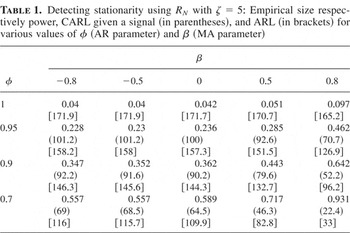
where φ and β are parameters and {en} i.i.d. N(0,1) innovations. The parameter values were chosen to be φ = 1, 0.95, 0.9, 0.7 and β = −0.8, −0.5, 0, 0.5, 0.8. We investigate the following quantities: First, size and power of the test that rejects H0 if the monitoring procedure gives a signal. Second, the average run length (ARL) defined as E(RN) and

, respectively, i.e., the average number of observations until we get a signal. Additionally, we provide the conditional ARL (CARL) given that the procedure gives a signal defined as, e.g., E(RN|RN < N). That quantity informs us how fast the procedure reacts if it reacts at all. We use a maximum sample size of N = 250. The bandwidth was chosen as h = 50. Simulated asymptotic critical values were used with ζ = N/h = 5 to attain a nominal rejection probability of 5%. The Gaussian and Epanechnikov kernels were investigated, which attach smaller weights to past summands than to more current ones. We found by simulations not reported here that the start of monitoring, k, should be proportional to h, and k = 1.5h yields a reasonable rule of thumb for ζ = 5.
Table 1 presents our results for the proposed procedure RN to detect stationarity, using the Epanechnikov kernel for weighting. Here H0 : I(1)-unit root is given by φ = 1. The results are generally supportive of the theory developed in the paper. We do not report the results for the Gaussian kernel, because they were quite similar. The first three rows present the actual sizes for different values of β. It can be seen that there is only a slight size distortion, similar to the results for the KPSS fixed-sample test. The remaining rows provide power estimates, CARLs, and ARLs. Overall, it appears that the monitoring approach provides a powerful method to detect stationarity quickly, as can be seen from the CARL values in parentheses. In many cases stationarity can be detected very early, and it is not necessary to wait until the time horizon N.
Detecting stationarity using RN with ζ = 5: Empirical size respectively power, CARL given a signal (in parentheses), and ARL (in brackets) for various values of φ (AR parameter) and β (MA parameter)

We next consider the properties of the procedure

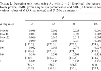
to detect a unit root. Here H0 : I(0)-stationarity corresponds to |φ| < 1 in our simulation model. For the Newey–West estimator we have to choose the lag truncation parameter m. We considered the following choices of m as a function of the (current) sample size: m3 = [lfloor ]0.75n1/3 + 0.5[rfloor ], m4 = [lfloor ]4(n/100)1/4 + 0.5[rfloor ], and m12 = [lfloor ]12(n/100)1/4 + 0.5[rfloor ] with n = [lfloor ]Nκ[rfloor ],…,RN ≤ N denoting the time point where the estimator has to be calculated. The rules m4 and m12 have also been used by Kwiatkowski et al. (1992); for m3 see Stock and Watson (2003, eqn. 13.17). For φ = 0 and β = −0.8, −0.5, 0, 0.5 we simulated the type I error for all choices of m. As can be seen from the top rows of Table 2, the difference seems negligible. For the remaining cases given by φ = 0.2, 0.6, 0.9, 1 we used m4. The last three rows of the table provide the performance to detect the unit root given by φ = 1. Overall, the empirical rejection rates and ARL/CARL values indicate that for moderate positive autocorrelation (0 ≤ φ ≤ 0.6) the procedure has moderate size distortion. But, as expected, for φ close to 1 the procedure overreacts. The power is uniformly high for all values of β studied here.
Detecting unit roots using with ζ = 5: Empirical size respectively power, CARL given a signal (in parentheses), and ARL (in brackets), for various values of φ (AR parameter) and β (MA parameter)

5.2. Change-Point Models
We also investigated the performance of the detection methods RN and

in change-point models. It is of particular interest to study the influence of the bandwidth h on the performance. To evaluate the rule RN (detection of stationarity), we used the following specification of the change-point model given in the introduction:

with N = 250. The {εt} are i.i.d. N(0,1)-innovations. The change-point parameter ϑ is chosen as ϑ = 0.1, 0.5, 0.75, and the bandwidth as h = 125, 50, 25.
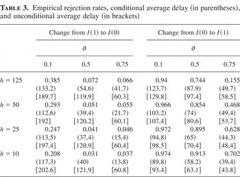
Table 3 reports power, the average delay, defined as E max(RN − [lfloor ]Nϑ[rfloor ],0), and the conditional average delay given the method provides a signal, defined as E(RN|RN < N) − [lfloor ]Nϑ[rfloor ], which informs us how quickly the procedure reacts if it reacts at all. It can be seen that there is only a negligible effect of the bandwidth h on the average delay, but a remarkable positive effect on the conditional average delay and the statistical power to reject the unit root hypothesis. Comparing h = 125 with h = 50 for ϑ = 0.1 and ϑ = 0.5 indicates that large bandwidths provide high overall power but the signal often comes late. To detect the change early smaller bandwidths seem to be better. Comparing with h = 10 shows that CARL increases again. It seems that for the setting studied here values between 25 and 50 provide reasonable results.
Empirical rejection rates, conditional average delay (in parentheses), and unconditional average delay (in brackets)

To investigate the detection rule

(detection of a unit root), we used the same change-point model as before but with φn = 0.6 if n < [lfloor ]Nϑ[rfloor ] and φn = 1 if n ≥ [lfloor ]Nϑ[rfloor ]. This means that before the change the process is AR(1) with autoregressive parameter 0.6 and after the change we are given a pure random walk. The parameter ϑ was chosen as before, and h = 125, 50, 25, 10. As can be seen from the right-hand side of Table 3, the detection performance is excellent in terms of power, average delay, and conditional average delay. Results for h = 5 were almost identical to h = 10 and are therefore omitted. Overall, small bandwidths increase the power substantially and yield smaller delays.
5.3. An Example
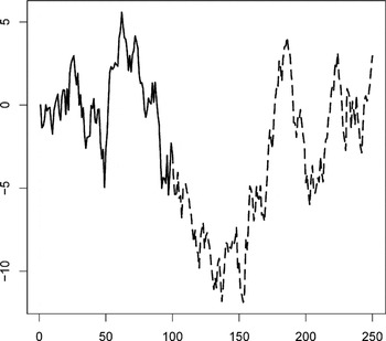
Figure 1 illustrates the detection performance of the proposed procedure for a time series of length 250 that has a change point. The first 100 observations follow an AR(1) with coefficient φ = 0.8. After the change point given by ϑ = 0.4, the series is a random walk (φ = 1). We applied the procedure

using the Epanechnikov kernel, bandwidth h = 25, the lag selection rule m4, and an asymptotic 5% control limit using ζ = 10. The change is detected at observation 167.

A time series with a change point at observation 100 where the AR coefficient changes from 0.8 to 1. The change is detected at observation 161.
6. SOFTWARE
User-friendly and platform independent JAVA software implementing the proposed methods, particularly providing asymptotic control limits, and example data sets can be downloaded from the author's Web page.
7. CONCLUSIONS
Monitoring rules to detect stationarity and unit roots quickly based on a kernel-weighted process related to the KPSS statistics are studied. Limiting distributions under various distributional assumptions including local-to-unity and change-point models are established. Simulations indicate that the procedures share the moderate size distortion of the KPSS test, but due to its weighting scheme controlled by a bandwidth parameter h the reaction performance is substantially improved. Both changes from I(0) to I(1) and changes from I(1) to I(0) can be detected very early in many cases, if h is chosen appropriately.