2.1. The structure design and working principle

The schematic of VSTCA, which integrates a tensegrity-based joint with MACCEPA, is shown in Figure 1. This joint consists of a fixed part, a follower member, two axial elastic elements, and four radial elastic elements. The materials of these elastic elements are selectable from elastic thread (e.g., fishing line), linear spring, artificial muscle, or shape memory alloy. By individually tensioning each element, an antagonistic tension network is formed, creating a floating connection between the fixed part and the follower member. The MACCEPA structure is assembled from steering motor A, steering motor B, strings, springs, the fixed part, and the follower member. Steering motor A drives the joint’s rotation, while steering motor B adjusts the pre-tension in the spring, providing precise control over the rotational stiffness of VSTCA. The rotation axis of the tensegrity-based joint is aligned with that of the MACCEPA structure.

Figure 1.

The sketch of VSTCA.

The VSTCA is fundamentally a tensegrity structure based on a prestressed elastic system in a rotational singular configuration [Reference Azadi, Behzadipour and Faulkner35]. The internal forces in this configuration are fully dedicated to generating rotational stiffness. By actively adjusting the spring pre-tension force via steering motor B, the mechanism’s stiffness can be tuned both effectively and simply. Under these conditions, the adjustable range of the active stiffness depends solely on the mechanism’s strength and dimensions. On the other hand, as the VSTCA rotates, positional changes alter the internal forces in the elastic elements of the tension network, thereby affecting the joint’s passive stiffness. The coupling between active and passive stiffness influences the overall controllability of the joint stiffness. A detailed stiffness analysis for VSTCA is provided in Section 2.2.

2.2. Stiffness analysis of VSTCA

Figure 2 illustrates the connection of the elastic component in the VSTCA. The coordinate system Oxyz is established, with the origin O located a distance h from the base of the follower member. For a tensegrity-based joint, the axial elastic elements l ₁ and l ₂ are anchored at points A ₁ B ₁ and A ₂ B ₂, respectively. Meanwhile, the radial elastic elements l ₃∼l ₆ are attached at points C ₁ D ₁, C ₂ D ₁, C ₃ D ₂, and C ₄ D ₂, respectively. c denotes the circumradius of points C ₁∼C ₄, while γ represents the acute angle formed between these points and the y-axis. The elastic coefficient of l ₁∼l ₆ is represented by k ₁. The left end E of the MACCEPA structure is fixed to the fixed part, and the right end J is secured to the follower member. Points E, D ₁, and D ₂ are collinear. Links EF and IJ serve as the arms of steering motors A and B, with lengths L _A and L _B, respectively. Point G represents a fixed hole on the follower member. The distance from point J to the line A ₁ A ₂ (namely GJ) is L _J . A spring with elastic coefficient k ₂ is attached to points F and G via a string at both ends.

Figure 2.

Schematic of the elastic element connections.

Figure 3.

Three variants of the MACCEPA structure. (Top: initial state, bottom: motion state).

The MACCEPA structure features several variants designed for different application scenarios, as shown in Figure 3. We refer to these structures in Figure 3 as Variant 1, Variant 2, and Variant 3, respectively. In Variant 1 (also shown in Figure 2), the spring is positioned between points F and G, offering a space-saving design ideal for multi-joint systems. Variant 2 places the spring between points G and I. Variant 3 is a passive variable stiffness structure, where the arm EF rotates to pre-tension the spring. The rotational stiffness of link IJ, which rotates under external force, is determined by the rotation angle of arm EF. Q. Zhong et al. utilized this variant to regulate the stiffness of a robotic tuna’s tail fin [Reference Zhong, Zhu, Fish, Kerr, Downs, Bart-Smith and Quinn36]. These three variants will be used in Sections 2.2 and 3. Despite the structural differences, all variants follow the same analytical methods and operate based on the same variable stiffness principle. The working principle of the MACCEPA structure is analyzed using Variant 1 as a representative case.

Initially, steering motor B rotates by an angle $\beta$ , producing a pre-tension force p in the spring. When the mechanism moves, that is, when steering motor A rotates by a certain angle, the internal force of the spring is:

(1) \begin{align} F&=k_{2}\biggl[\sqrt{L_{\mathrm{A}}^{2}+\left(H_{0}+H\right)^{2}-2L_{\mathrm{A}}\left(H_{0}+H\right)\cos \alpha }-\left(H_{0}+H-L_{\mathrm{A}}\right)\nonumber\\ &\quad+\sqrt{L_{J}^{2}+L_{\mathrm{B}}^{2}-2L_{J}L_{\mathrm{B}}\cos \beta }-\left(L_{J}-L_{\mathrm{B}}\right)\biggr]\end{align}

where H is the axial separation between A ₁ and B ₁ along the z-axis and H ₀ is the perpendicular distance from the line segment D ₁ D ₂ to the fixed part, as shown in Figure 2. Thus, the sum of H and H ₀ equals the distance between points E and G, as shown in Figure 3. α denotes the angle between link EF and the follower member. α decreases with increasing k ₂.

The mechanism’s rotational stiffness K _M is derived through the law of sines.

(2) \begin{equation} K_{M}=\partial T/\partial \alpha =\partial \left[FL_{\mathrm{A}}\left(H_{0}+H\right)\sin \alpha /\sqrt{L_{\mathrm{A}}^{2}+\left(H_{0}+H\right)^{2}-2L_{\mathrm{A}}\left(H_{0}+H\right)\cos \alpha }\right]/\partial \alpha \end{equation}

where T is the torque applied at point G of the follower member.

In practical, α is a small angle (generally less than 15 $^{\circ}$ ) for two reasons. First, VSTCA joints are usually used in multiples to construct robotic arms or bio-inspired structures. As a result, the rotation angle required from an individual joint is reduced, leading to a smaller α. Second, when the external load and joint stiffness are properly matched – meaning high stiffness for large loads or low stiffness for small loads – α tends to remain small. Therefore, the expression for K _M simplifies to the following equation.

(3) \begin{equation} K_{M}=\frac{L_{\mathrm{A}}\left(H_{0}+H\right)}{H_{0}+H-L_{\mathrm{A}}}\cdot k\left[\sqrt{L_{J}^{2}+L_{\mathrm{B}}^{2}-2L_{J}L_{\mathrm{B}}\cos \beta }-\left(L_{J}-L_{\mathrm{B}}\right)\right]=\mu p \end{equation}

where μ represents the stiffness amplification factor, which depends solely on the mechanism’s parameters, and p is the pre-tension force in the spring. This implies that when α is small, the rotational stiffness is approximately linear with respect to the pre-tension force. Furthermore, the rotational stiffness is independent of the rotation angle.

Next, the stiffness of VSTCA is analyzed. Based on the positions of the elastic components, vector expressions for both the axial and radial elastic elements are obtained.

(4) \begin{equation}l_i=RA_i-B_i (i = 1, 2), l_i=RD_j-C_k (i = 3 ~ 6, j = 1, 1, 2, 2, k = 1 ~ 4)\end{equation}

where R denotes the rotation matrix describing the movement of the follower member relative to the fixed part. The vectors A _i , B _i , D _j , and C _k extend from point O to points A _i , B _i , D _j , and C _k , respectively. Thus, the Jacobian matrix J is

(5) \begin{equation} \boldsymbol{J}=\left[\begin{array}{c@{\quad}c@{\quad}c@{\quad}c@{\quad}c@{\quad}c} \boldsymbol{l}_{n\mathit{1}} & \boldsymbol{l}_{n\mathit{2}} & \boldsymbol{l}_{n\mathit{3}} & \boldsymbol{l}_{n\mathit{4}} & \boldsymbol{l}_{n\mathit{5}} & \boldsymbol{l}_{n\mathit{6}}\\ \boldsymbol{R}\boldsymbol{A}_{1}\times \boldsymbol{l}_{n\mathit{1}} & \boldsymbol{R}\boldsymbol{A}_{2}\times \boldsymbol{l}_{n\mathit{2}} & \boldsymbol{R}\boldsymbol{D}_{1}\times \boldsymbol{l}_{n\mathit{3}} & \boldsymbol{R}\boldsymbol{D}_{1}\times \boldsymbol{l}_{n\mathit{4}} & \boldsymbol{R}\boldsymbol{D}_{2}\times \boldsymbol{l}_{n\mathit{5}} & \boldsymbol{R}\boldsymbol{D}_{2}\times \boldsymbol{l}_{n\mathit{6}} \end{array}\right]_{6\times 6} \end{equation}

where l _ni represents the unit vector of l _i .

The Jacobian matrix enables derivation of the VSTCA stiffness matrix K according to the stiffness theory for parallel mechanisms [Reference Azadi, Behzadipour and Faulkner35,Reference Chakarov37].

(6) \begin{equation} \boldsymbol{K}=\frac{\partial \boldsymbol{F}}{\partial \boldsymbol{x}}=\frac{\partial \boldsymbol{J}^{\mathrm{T}}\boldsymbol{f}}{\partial \boldsymbol{x}}=\boldsymbol{J}^{\mathrm{T}}\boldsymbol{k}_{\mathit{s}}\boldsymbol{J}+\frac{\partial \boldsymbol{J}^{\mathrm{T}}}{\partial \boldsymbol{x}}\boldsymbol{f}=\boldsymbol{K}_{\mathrm{E}}+\boldsymbol{K}_{\mathrm{G}} \end{equation}

where F and f represent the external load vector applied to the structure and the pretension force vector of the elastic elements, respectively. k _s is a diagonal matrix of the elastic elements’ material stiffness, and x is the generalized coordinate. The stiffness matrix K consists of two components: the material stiffness or passive stiffness K _E, corresponding to the joint’s stiffness in its initial prestress-free state; and the antagonistic stiffness or active stiffness K _G, arising from the repositioning ( $\partial \boldsymbol{J}^{\mathrm{T}}/\partial \boldsymbol{x}$ ) and the internal forces of elastic elements.

Since the VSTCA primarily operates within the y-O-z plane, the stiffness matrix reduces to a 3 × 3 planar stiffness matrix. When the joint is in its neutral position, where $\phi$ = 0, K is given by:

(7) \begin{equation} \boldsymbol{K}=\left[\begin{array}{c@{\quad}c} \boldsymbol{K}_{Tran} & \boldsymbol{K}_{CP}^{T}\\ \boldsymbol{K}_{CP} & \boldsymbol{K}_{Rot} \end{array}\right]=\left[\begin{array}{c@{\quad}c@{\quad}c} K_{y} & 0 & K_{y\varphi }\\ 0 & K_{z} & 0\\ K_{y\varphi } & 0 & K_{\varphi } \end{array}\right] \end{equation}

where K _Tran , K _Rot , and K _CP are the translational stiffness, rotational stiffness, and translational-rotational coupling stiffness of VSTCA, respectively. K _y , K _z , and K $_\phi$ denote the translational stiffness in the y-direction, z-direction, and rotational stiffness around the $\phi$ -axis, respectively. K _yφ denotes the coupling stiffness between the y-direction and the $\phi$ -axis. The expressions of K _y , K _z , and K $_\phi$ are provided in Eqs. (8)–(11).

(8) \begin{equation} K_{y}=4k_{1}c^{2}\cos ^{2}\beta /{\mathit{l}_{\mathit{e}}}^{2}+2\tau _{a}/H+4\tau _{\mathit{r}}\left({\mathit{l}_{e}}^{2}-c^{2}\cos ^{2}\beta \right)/{\mathit{l}_{e}}^{3}\\[-12pt] \end{equation}

(9) \begin{equation} K_{z}=k_{1}\left(2+4H_{0}^{2}/{l_{e}}^{2}\right)+\mathit{k}_{2}+4\tau _{r}\left({l_{e}}^{2}-H_{0}^{2}\right)/{l_{e}}^{3}\\[-12pt] \end{equation}

(10) \begin{equation} K_{y\varphi }=4k_{1}c^{2}\cos ^{2}\beta \left(H+H_{0}-h\right)/{l_{e}}^{2}-2\tau _{a}\mathit{h}/\mathit{H}+4\tau _{\mathit{r}}\left({\mathit{l}_{e}}^{2}-c^{2}\cos ^{2}\beta \right)\left(H+H_{0}-h\right)/{\mathit{l}_{e}}^{3}\\[-12pt] \end{equation}

(11) \begin{equation} K_{\varphi }=K_{y}\left(\mathit{h}-\mathit{H}-H_{0}\right)^{2}+2\tau _{a}H_{0}+K_{M}\\[-12pt] \end{equation}

where l _e refers to the length of the radial elastic element. $l_{e}=\sqrt{c^{2}+d^{2}+{H_{0}}^{2}-2cd\sin ^{2}\mathit{\gamma }}$ . τ _r and τ _a are the prestress of the radial and axial elastic elements. The terms related to k in these equations correspond to the material stiffness, while the remaining terms represent the antagonistic stiffness.

To decouple the stiffness in the y-, z-, and $\phi$ -directions, the coupling stiffness term K _yφ must be set to zero. Consequently, the following condition is obtained.

(12) \begin{equation} h=H+H_{0}-2\left(H+H_{0}\right)\tau _{a}/K_{y} \end{equation}

When k ₁ is a large value, the last term in Eq. (12) becomes negligible, resulting in h=H+H ₀. In this case, point O becomes the decoupling center for the three degrees of freedom, effectively serving as the virtual rotation center of the VSTCA. This configuration is justified because, for the VSTCA to function as a rotational joint, translational motion in the y- and z-directions must be constrained. A large k ₁ ensures high stiffness in both the y- and z-directions.

When h = H + H ₀, the first term in K $_\phi$ is zero, the second term represents the antagonistic stiffness associated with prestress, and the third term corresponds to the rotational stiffness generated by the MACCEPA (see Eq. (3)). Simultaneous activation of the second and third terms would introduce interference in active stiffness regulation. Moreover, employing antagonistic stiffness for stiffness adjustment in the VSTCA faces two challenges: the difficulty in precisely controlling internal forces and the limited range and controllability of stiffness adjustment. Therefore, during joint assembly, τ _a should be minimized to approach zero, deactivating the second term. Under these conditions, K $_\phi$ = K _M, meaning that MACCEPA fully assumes the function of active stiffness regulation for the VSTCA. The internal forces serve two primary roles: (1) maintaining structural stability and (2) enhancing translational stiffness via Eqs. (8) and (9), effectively approximating rigid constraints.

In practical applications, maintaining a perfectly stable virtual rotation axis is challenging. Since k ₁ cannot be infinitely large, the VSTCA will experience slight translational displacement, resulting in a deviation of the center of rotation. B. Chen et al. evaluated a compliant joint’s equivalence to a rigid joint using a dimensionless axis drift metric [Reference Chen, Jiang, Liu and Lu33]. Their research confirmed that the tensegrity-based joint maintains good equivalence within ≤5% dimensionless shaft drift.

When the joint is not in its neutral position (φ ≠ 0), substituting the condition h = H+H ₀ into Eq. (6) yields the relationship between K $_\phi$ and $\phi$ .

(13) \begin{equation} K_{\varphi }\left(\varphi \right)=2k_{1}\left(\mathit{h}\mathit{H}_{0}\sin \varphi /H\right)^{2} \end{equation}

Figure 4 illustrates how K $_\phi$ varies with the pre-tension angle $\beta$ and the rotation angle $\phi$ of the joint. The structural parameters are as follows: a = 50 mm, c = 46.5 mm, d = 35 mm, L _A = L _B = 20 mm, L _J = 67 mm, H = 61 mm, H ₀ = 3 mm, γ = 65 $^{\circ}$ , k ₁ = 6670 N/m, and k ₂ = 667 N/m. Figure 4(a) presents the exact stiffness calculations based on Eq. (2) for α = 5 $^{\circ}$ , 10 $^{\circ}$ , and 15 $^{\circ}$ , as well as the approximate stiffness calculation from Eq. (3) for α = 5 $^{\circ}$ . The four curves demonstrate a strong level of consistency. By redesigning the structural parameters, the mechanism can achieve a broader range of stiffness variation. As shown in Figure 4(b), K $_\phi$ increases with the joint rotation angle but remains consistently within a small range, rendering its influence negligible. For multi-joint robots, the rotation angle of each joint would be reduced. For instance, a tail-beat amplitude of 0.23 body lengths can be achieved in a four-joint robotic fish with merely 3.2 $^{\circ}$ of rotation per joint. Under such conditions, joint stiffness remains within 0–2 × 10⁻³ N·m/rad, exerting negligible impact on the overall stiffness. Consequently, the tensegrity-based joint exhibits kinematic equivalence to a conventional rotational pair throughout its entire range of motion.

Figure 4.

Stiffness variation in response to changes in (a) the rotation angle of steering motor B and (b) the rotation angle of the joint.

2.3. Experiment platform

The design drawing and physical model of a single-joint VSTCA are shown in Figure 5. The physical model is mounted on a 400 mm (L) × 200 mm (W) × 10 mm (T) acrylic sheet, which is fixed onto an aluminum extrusion frame measuring 400 mm (L) × 200 mm (W) × 550 mm (H). Both steering motors utilize RGD01L models powered by 7.4 V lithium batteries. Key specifications at 7.4 V include a maximum rotation angle of 180 $^{\circ}$ , a torque output of 15 kg·cm, and an operating speed of 0.1 s/60 $^{\circ}$ . The fixed part and follower member are fabricated by 3D printing with photosensitive resin, while the elastic elements and strings are secured with metal fasteners. The VSTCA designed for the experiments exhibits a joint motion range of ±25 $^{\circ}$ with a stiffness adjustment range of 0–0.63 N·m/rad. The stiffness adjustment range can be tuned for specific requirements by modifying structural dimensions, spring stiffness, and pre-tension force.

Figure 5.

The design drawing (a) and physical model (b) of a single-joint VSTCA.

Compared to Figure 1, the primary modification in Figure 5 is the adoption of Variant 2 of the MACCEPA, which allows for easier monitoring of spring length changes using an MV-UG050GM/C industrial camera (100 fps frame rate, 800 × 600 resolution) mounted 0.5 m above the mechanism. The measurement system employs monocular vision technology to capture the motion sequences, with the camera’s optical axis aligned orthogonally to the image plane. Through image processing, marker points on a calibration ruler are extracted to obtain pixel coordinates, thereby establishing a pixel-to-length conversion ratio. This approach effectively simplifies the camera calibration process. By detecting the pixel coordinates of the spring’s endpoints and applying the calibrated conversion ratio, the physical length change of the spring is computationally determined. The instantaneous central axis of the follower member can also be recognized by finding the points A ₁ and B ₁ shown in Figure 2, enabling the measurement of the joint rotation angle.

2.4. Experimental validation

To investigate the impact of the angle $\beta$ on joint stiffness, a controlled experiment was conducted with $\beta$ set to 15 $^{\circ}$ , 45 $^{\circ}$ , and 75 $^{\circ}$ . The camera captured the motion of the VSTCA driven by steering motor A. From the recorded image sequences, data on spring length and joint rotation angle (denoted as θ _J ) were extracted, allowing for the calculation of the angle α, torque T, and stiffness K (see Figure 6). In this experiment, the maximum rotation angle of steering motor A (denoted as θ _A ) is set to 30 $^{\circ}$ . Phase lag in stiffness modulation becomes pronounced beyond 3 Hz driving frequency, as quantified in preliminary trials. Hence, the driving frequency of steering motor A was set to 1 Hz. The spring’s elastic coefficient k was 590 N/m, and the length ratio λ = L _A/h was 4 (with the definitions of L _A and h provided in Section 2.1). Figure 6(a) shows that, when θ _A holds constant, θ _J increases slightly as $\beta$ increases, gradually approaching θ _A . At the same time, the angle α (the difference between θ _A and θ _J ) decreases with increasing $\beta$ , tending toward zero. For $\beta$ values of 15 $^{\circ}$ , 45 $^{\circ}$ , and 75 $^{\circ}$ , the maximum values of θ _J are 20.3 $^{\circ}$ , 22.8 $^{\circ}$ , and 24.7 $^{\circ}$ , respectively, while the corresponding maximum values of α are 9.7 $^{\circ}$ , 7.2 $^{\circ}$ , and 5.3 $^{\circ}$ . In general, α is negatively correlated with the load on the follower member and positively correlated with the spring’s pre-tension (i.e., the angle $\beta$ ). As illustrated in Figure 6(c), the experimentally measured stiffness values fluctuate slightly around the theoretical predictions derived from Eq. (2), with little variation as θ _A changes. When $\beta$ increases from 15 $^{\circ}$ to 75 $^{\circ}$ , the stiffness increases by approximately 8.6 times. 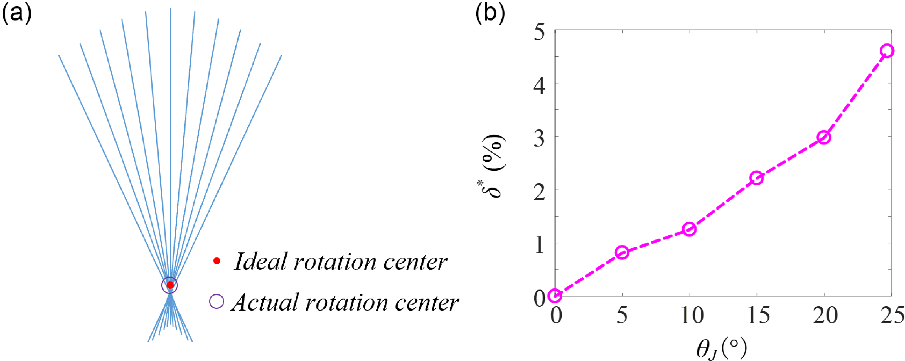Theoretically, if $\beta$ is further increased to 150 $^{\circ}$ , the stiffness is expected to rise by about 15.7 times, demonstrating the VSTCA’s ability to achieve a wide range of stiffness adjustment. This experiment and the corresponding calculations omit the small rotational stiffness generated when the tensegrity-based joint is not in its neutral position. As a result, the actual rotational stiffness is likely slightly higher than the theoretical value. However, this does not affect the overall conclusions. During the VSTCA’s rotation, the maximum non-dimensional axial drift was measured at 4.7%, satisfying the joint equivalence requirement and highlighting the joint’s low axial drift characteristic.

Figure 6.

The variations of (a) the joint rotation angle θ_J and the angle α, (b) torque T acting on the joint, and (c) the joint’s rotational stiffness K, with different driving angles θ_A of steering motor A.

Figure 7(a) depicts the instantaneous central axis locations of the follower member during the experiment for θ _J = 25 $^{\circ}$ to help observe the variation in the joint rotation center. Figure 7(b) plots the computed dimensionless shaft drift δ ^* of the structure for different θ _J , revealing a rise to a maximum of 4.7% with increasing the follower member’s rotation angle. This low shaft drift characteristic demonstrates compliance with the joint equivalence requirement.

Figure 7.

The joint rotation center variation (a) and its dimensionless axis drifts (b).

To examine the variation in joint stiffness across a wide range of angle α, the follower member was fixed with a holder, effectively simplifying the VSTCA into a basic MACCEPA mechanism, where θ _A = α. This means that the characteristics among joint torque, stiffness, and deflection angle are investigated under static conditions. Additionally, to explore the impact of the length ratio λ on the mechanism’s stiffness, a controlled experiment was conducted with λ set to 1.5, 2, 3, and 4. The different holes in the overhanging arm of the follower member (as shown in Figure 5) define the distance between the fixed part and the follower member, thereby determining the value of h. In this experiment, the spring’s elastic coefficient was 220 N/m, and the maximum α was set to 60 $^{\circ}$ . Figure 8 illustrates the variation of torque and stiffness with α at different length ratios, where ‘ER’ denotes experimental results and ‘TV’ represents theoretical values. The experimental data closely match the theoretical predictions. For λ = 1.5, stiffness decreases sharply with increasing α, showing a 76% reduction as α progresses from 0 $^{\circ}$ to 60 $^{\circ}$ . When λ = 2, stiffness first remains nearly constant for α between 0 $^{\circ}$ and 15 $^{\circ}$ , followed by a marked 41% decrease beyond that threshold. For λ = 3 and 4, stiffness initially increases and then decreases with α, but the overall variation is considerably smaller than in the cases of λ = 1.5 or 2. Among all cases, the smallest stiffness fluctuation occurs at λ = 3. These results suggest that both excessively small and large length ratios lead to greater stiffness fluctuations. Theoretically, there exists an optimal ratio at which stiffness remains relatively stable when α is small.

Figure 8.

Torque and stiffness variations with respect to the angle α for different λ ratios.

Figure 9.

Serial mechanism configuration. (a) Design drawing, (b) Physical model, (c) Locomotion performance.

Experimental studies on the single-joint VSTCA confirmed its capacity for wide-range stiffness modulation, as well as the decoupling of rotation angle from rotational stiffness. The next step involves extending the actuator to multi-joint mechanisms, further enhancing its potential for diverse applications.

3.1. Serial mechanism configuration

The multi-joint serial mechanism is modularly constructed based on the VSTCA described in Section 2. Figure 9 presents both the design drawing and physical model of the four-joint serial mechanism. To achieve a more compact configuration, Variant 1 of the MACCEPA is employed for variable stiffness control. Each joint is equipped with two steering motors: one to control the joint’s rotation angle (referred to as the active drive servo) and the other to regulate its rotational stiffness (referred to as the pre-tensioning servo). Rubber rollers are mounted beneath each joint, allowing the mechanism to propel forward through friction. This configuration differs from the multi-joint swimming platform developed by M. Ziegler et al. [Reference Ziegler, Hoffmann, Carbajal and Pfeifer24] in two key aspects: the use of tensegrity-based joints and the ability of each joint to drive actively. By coordinating the rotation angles of these servos, the mechanism is capable of generating oscillatory motion and selectively distributing stiffness along the structure.

Figure 10.

Wire-driven mechanism configuration. (a) Design drawing. (b) Wire-driven principle.

The pre-tensioning servo’s rotation angle is set to 10 $^{\circ}$ , 20 $^{\circ}$ , 30 $^{\circ}$ , and 40 $^{\circ}$ to showcase the variations of the mechanism stiffness. The maximum rotation angle of the active drive servo θ _A is set to 30 $^{\circ}$ , 45 $^{\circ}$ , and 60 $^{\circ}$ . Aside from phase differences, all four active drive servos share identical parameter settings, resulting in a near-sinusoidal oscillatory motion. Figure 9(c) shows how the mechanism’s average forward speed varies with different combinations of drive angle θ _A and pre-tensioning angle $\beta$ . When θ _A is 30 $^{\circ}$ or 45 $^{\circ}$ , the forward speed increases as $\beta$ grows, reaching up to a 73% improvement. The peak forward speed observed is approximately 31 mm/s, indicating that greater stiffness enhances. However, when $\beta$ is held constant and θ _A is varied, the speed increase becomes less pronounced at higher θ _A . This is likely due to larger lateral oscillations diminishing the forward component of motion. At θ _A = 60 $^{\circ}$ , the forward speed first increases and then decreases with increasing $\beta$ , suggesting that at high oscillation amplitudes, the interaction between lateral displacement and stiffness introduces a more complex influence on propulsion performance.

In this experiment, the dimensionless axial drifts of the joints increase with larger active drive angles. At θ _A values of 45 $^{\circ}$ and 60 $^{\circ}$ , the drift partially exceeds the 5% design tolerance. A more effective approach would be to increase the number of serial joints, thereby reducing the required active drive angle per joint and better preserving the functional equivalence to rigid joints. To minimize structural and control complexity, only four joints were used in this study, with a primary focus on qualitative analysis. As such, the joint equivalency requirement was not strictly enforced.

This variable-stiffness, multi-joint oscillatory propulsion mechanism demonstrates strong potential for applications in areas such as pipeline inspection and bio-inspired underwater propulsion (e.g., robotic snakes or anguilliform robotic fish). Optimizing the stiffness distribution along serial joints can further enhance its propulsion performance.

3.2. Wire-driven mechanism configuration

The wire-driven mechanism configuration is illustrated in Figure 10(a). This design features a fish-inspired serial tensegrity-based structure with variable stiffness implemented at the terminal joint. The mechanism comprises four tensegrity-based joints: the first three joints replicate the fish body and enable controlled bending through an active drive servo, while the final joint, equipped with an online variable stiffness mechanism based on Variant 3 of the MACCEPA, mimics the caudal fin with adjustable rotational stiffness. To enhance compactness and facilitate integration within the internal cavity of a robotic fish’s head, the pre-tensioning servo, spring, and active drive servo are all placed at the front of the mechanism.

The bending process of the wire-driven mechanism is depicted in Figure 10(b). Wires are routed along both sides of the mechanism, connecting the arm of the active drive servo to excitation points. The driving torque generated by the servo is transmitted through the wire to these excitation points, driving rotational displacement in each joint to produce controlled bending deformation of the mechanism. Assuming identical rotation angles at all joints, the wire length variations on both sides between adjacent joints are described mathematically by:

(14) \begin{equation} \left\{\begin{array}{l} {\unicode[Arial]{x0394}} \mathit{w}_{l}=-d\sin \left({\Phi} /2N\right)-2\mathit{h}\sin ^{2}\left({\Phi} /4N\right)\\[6pt] {\Phi} \mathit{w}_{r}=d\sin \left({\Phi} /2N\right)-2\mathit{h}\sin ^{2}\left({\Phi} /4N\right) \end{array}\right. \end{equation}

where Δw _l and Δw _r denote the wire length variation of the left side and right side, respectively. N represents the number of joints in the mechanism. h indicates the gap between adjacent joints. d is the width of bilateral wires.

Given the small magnitude of Φ/4N, the quadratic term in Eq. (14) is neglected. The total change in the wire is controlled by the rotation of the servo arm, which is expressed as the following equation.

(15) \begin{equation} {\unicode[Arial]{x0394}} \mathit{w}_{l}=-{\unicode[Arial]{x0394}} \mathit{w}_{r}=-D\alpha /N \end{equation}

where D and α represent the length and the rotation angle of the servo arm, respectively. Therefore, the relationship between the servo’s rotation angle α and the bending angle of the end joint Φ is governed by Eq. (16).

(16) \begin{equation} {\Phi} =2N\cdot \arcsin \left(D\alpha /2Nd\right) \end{equation}

The variable stiffness principle has been detailed in Section 2.1. When applied to carangiform or thunniform robotic fish, hydrodynamic forces generated during body undulation induce a relative angle $\beta$ between the caudal fin and fish body, as shown in Figure 3. The rotational stiffness of the end joint is determined by the rotation angle α of the pre-tensioning servo and the elastic coefficient k of the spring. Figure 11 presents the bending states of the mechanism when the active drive servo rotates by 15 $^{\circ}$ , 30 $^{\circ}$ , and 45 $^{\circ}$ . Figure 12 gives simulation and experimental results for the three bending states. As the rotation angle of the active drive servo increases, the mechanism’s bending deformation correspondingly intensifies. The corresponding theoretical end angles calculated from Eq. (16) are 20.3 $^{\circ}$ , 40.6 $^{\circ}$ , and 61.1 $^{\circ}$ , while the experimental measurements are 23 $^{\circ}$ , 41.5 $^{\circ}$ , and 59 $^{\circ}$ , respectively. This demonstrates a good agreement between simulation and experimental results. Since the experiment was conducted in air without any external load, the end joint moved in unison with the third joint, resulting in no relative angle between them.

Figure 11.

Bending states of the mechanism at different active driving angles: (a) 15^°, (b) 30 ^°, (c) 45^°.

Figure 12.

Simulation and experimental results for the three bending are states shown in Figure 11.

3.3. Direct-drive mechanism configuration

The direct-drive mechanism is illustrated in Figure 13(a). Inside the mechanism is a VSTCA. To conserve space, the mechanism utilizes Variant 1 of the MACCEPA (see Figure 1). Externally, the mechanism consists of four serially connected tensegrity-based joints, which are linked to the internal structure via a spar that moves freely through a central hole in the follower member of the fourth joint. The active drive servo rotates the internal mechanism’s follower member, directly driving the spar to bend the external joints. The design imposes limits on the maximum rotation angle of each external joint. Without these constraints, the entire mechanism would primarily rotate around the fixed part of the first joint. Unlike the wire-driven mechanism described in Section 3.2, where all joints rotate simultaneously by the same angle, the joints in this mechanism bend sequentially.

Figure 13.

The direct-drive mechanism configuration. (a) Design drawing, (b) Motion trajectory of the spar end, (c) Bending state of the mechanism.

The specific bending pattern is achieved by coupling the active drive servo’s rotation angle with the maximum allowable rotation angles of the external joints, as illustrated in Figure 13(b). In this figure, O ₁, O ₂, O ₃, and O ₄ are the rotation centers for the first to fourth external joints, respectively. r ₁, r ₂, r ₃, and r ₄ denote the distances from the mechanism’s endpoint to the rotation centers of these joints, while θ ₁, θ ₂, θ ₃, and θ ₄ represent the maximum allowable rotation angles of each corresponding joint. The endpoint’s trajectory is composed of four distinct circular arcs. The first arc is centered at O ₁ with a radius r ₁ and angle θ ₁, and subsequent arcs follow the same pattern. Although the overall trajectory is not a perfect circular arc, it closely approximates one. When all the external joints reach their maximum rotation angles, the geometric relationships determine the active drive servo’s rotation angle.

Figure 13(c) shows the bending states of the mechanism. It clearly demonstrates that the axial bending of each joint closely aligns with the polyline O ₁ O ₂ O ₃ O ₄ shown in Figure 13(b), fulfilling the intended design objective. This mechanism, based on the principle of internal single-joint actuation with external multi-joint passive response, not only effectively integrates tensegrity-based joints with the MACCEPA structure but also enables the generation of specific motion trajectories with smooth and compliant motion characteristics. This design shows promising potential for applications in fields such as variable stiffness robotic arms and bio-inspired robotic fish. In the latter case, the spar functions as the spine, the internal variable stiffness module simulates the fish’s natural stiffness adjustment, and the four serially connected external tensegrity-based joints mimic the segmented structure of the fish body.