1 Introduction
This paper is the second in a two-part series investigating the combinatorics and geometry underlying Wilson loop diagrams in SYM
 $N=4$
theory. This series lays out several results about the relationship between Wilson loop diagrams and the positroid cells that give a CW complex structure to the positive Grassmannian. This paper is concerned with identifying which positroid cells correspond to which Wilson loop diagrams, and how this translates to a geometric tiling of a subspace of the positive Grassmannians.
In contrast, the first paper in this series focuses on combinatorial and matroidal properties of the Wilson loop diagrams. The main focus of that paper is on enumerating the positroid cells that are associated to Wilson loop diagrams with a fixed number of vertices and propagators, as well as counting the number of Wilson loop diagrams that map to the same positroid. The results of the first paper are not a prerequisite for this paper.
In recent years, there has been significant interest in understanding the geometry and combinatorics underlying the field theory SYM
 $N=4$
[Reference Agarwala and Marin-Amat8, Reference Arkani-Hamed and Trnka13, Reference Eden, Heslop and Mason20, Reference Galashin and Lam21, Reference Karp, Williams and Zhang25]. This started with the observation that BCFW diagrams, which represent the on shell interactions of this theory, correspond to plabic graphs [Reference Arkani-Hamed, Bourjaily, Cachazo, Goncharov, Postnikov and Trnka10]. Plabic graphs were introduced by Postnikov in [Reference Postnikov30, Section 11], and provide one of the many equivalent ways to classify the positroid cells of the positive real Grassmannian
 $\mathbb {G}_{\mathbb {R}, \geq 0}(k,n)$
. This led to the representation of the on shell integrals associated to this theory in terms of a geometric space (the Amplituhedron) embedded in
 $\mathbb {G}_{\mathbb {R}, \geq 0}(k,n)$
[Reference Arkani-Hamed and Trnka12, Reference Arkani-Hamed and Trnka13]. Moreover, integrands associated to the BCFW diagrams define a volume form on the Amplituhedron. This gives a novel and elegant interpretation of scattering amplitudes for this theory, as well as a means of greatly simplifying the calculations involved in traditional Feynman diagram approaches. Since then, there has been significant work devoted to understanding the volume form and its physical implications [Reference Arkani-Hamed, Thomas and Trnka11, Reference Galashin and Lam21].
Meanwhile, a different body of work has studied SYM
 $N=4$
theory from the point of view of Feynman integrals in twistor space [Reference Adamo, Bullimore, Mason and Skinner1, Reference Adamo and Mason3, Reference Boels, Mason and Skinner14, Reference Bullimore, Mason and Skinner16]. These integrals are calculated via holomorphic Wilson loops. As with the Amplituhedron, each Wilson loop represents the sum of a family of
 $N^kMHV$
Feynman diagrams. Each of the Feynman integrands in this sum associates a volume form to a convex space, parallel to the Amplituhedron [Reference Cachazo, Svrcek and Witten17, Reference Hodges24]. However, the geometric objects decomposing the Wilson loops are different from the geometric object decomposing the Amplituhedron.
Wilson loop diagrams, as we will study them, are objects given by a perturbative expansion of the holomorphic Wilson loop in twistor space. Classically, the interactions of the theory were studied as maximal helicity violating (MHV) diagrams, next-to-MHV diagrams, and so on (
 $N^kMHV$
diagrams) in momentum space. Adamo and Mason, in [Reference Adamo and Mason2], gave an elegant formulation for the
 $N^kMHV$
diagrams in twistor space. The Wilson loop diagram perspective of this paper is dual to this twistor representation of
 $N^kMHV$
diagrams. The objects are closely related and carry the same information. We choose to emphasize the dual perspective by our focus on the Wilson loop diagrams.
In [Reference Agarwala and Marin-Amat8], Agarwala and Marin-Amat uncovered a connection between the Wilson loop diagrams and positroids, defined as matroids that can be realized as an element of
 $\mathbb {G}_{\mathbb {R}, \geq 0}(k,n)$
. Other work has shown a connection between the volume filled by Wilson loop diagrams and the Amplituhedron [Reference Agarwala and Fryer5, Reference Eden, Heslop and Mason20]. Specifically, Marcott showed that the space parametrized by the Wilson loop diagrams is exactly the correct positroid cell in
 $\mathbb {G}_{\mathbb {R}, \geq 0}(k,n)$
, up to a set of measure zero [Reference Marcott27].
In the above work and elsewhere, it is clear that while the space parametrized by the Wilson loop diagrams is related to the Amplituhedron, they are not the same space, nor is a direct connection between the geometry of the Amplituhedron and the geometry of the Wilson loop diagrams known. For instance, it is conjectured that the Amplituhedron is orientable, whereas Agarwala and Marcott showed in [Reference Agarwala and Marcott7] that the space parametrized by the Wilson loop diagrams as a subspace of
 $\mathbb {G}_{\mathbb {R}, \geq 0}(k, n+1)$
can be seen as a nonorientable vector bundle over some submanifold of
 $\mathbb {G}_{\mathbb {R}, \geq 0}(k,n)$
. Furthermore, the cells associated to the Wilson loop diagrams are different from the cells associated to BCFW diagrams, which can be seen by comparing the results of [Reference Agarwala and Fryer5] and [Reference Karp, Williams and Zhang25]. Furthermore, the spaces in the two situations have different dimensions, as we will discuss further below, and examples show [Reference Heslop and Stewart23] that they do not relate by a coordinate projection or boundary map or other straightforward function. Nonetheless, from their common physical origin, it is believed that once the integrals over these spaces are taken, the results will parametrize related spaces [Reference Agarwala and Marin-Amat8, Reference Eden, Heslop and Mason20].
The Amplituhedron and the Wilson loop diagrams describe the scattering amplitudes from the same physical theory, but the Amplituhedron only captures the on shell portion, whereas the Wilson loop diagrams capture arbitrary kinematics. Both are related to positroids, and in this way, they have similar combinatorics, but these combinatorial objects manifest themselves differently in the two cases. For instance, square moves and merge-expand moves on the plabic graph give different graphical representations, hence parametrizations, of the same positroid cell in the Amplituhedron case. On the other hand, as we show in our companion paper [Reference Agarwala, Fryer and Yeats6], retriangulations of polygon dissections associated to Wilson loop diagrams give all the Wilson loop diagrams associated to the same positroid cell. Each distinct Wilson loop diagram associated to the same positroid cell gives a different parametrization [Reference Marcott27]. The deeper combinatorial and geometric connection between the Amplituhedron and the Wilson loop diagrams, which physics tells us should exist, remains to be uncovered in future work.
This paper continues the program of establishing concrete connections between the combinatorics of the Wilson loop diagram as determined by the physics, and the combinatorics of the associated positroid cell as identified in [Reference Agarwala and Marin-Amat8]. In this paper, we give an algorithm to read the Grassmann necklace, one of the standard combinatorial characterizations of the positroid cell, directly off the Wilson loop diagram. We also show that the positroid cells associated to Wilson loop diagrams are all
 $3k$
-dimensional, where k is the number of propagators in the diagram; by contrast, the BCFW cells are all
 $4k$
-dimensional [Reference Arkani-Hamed and Trnka13]. In [Reference Agarwala and Marcott7], the authors noted that the Wilson loop diagrams only correspond to positroid cells when the gauge vector is ignored. Including the gauge vector defines a
 $4k$
-dimensional subspace of
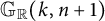 $\mathbb {G}_{\mathbb {R}}(k,n+1)$
.
As described above, each integrand associated to a Wilson loop diagram gives the volume of a convex polytope. However, each individual tree-level integral has singularities. These singularities are of two types: physical and spurious. The physical singularities come from special kinematical points, and we will not consider them in this paper. The spurious singularities come from zeros of the denominator of the integral, and hence are accessible to our combinatorial techniques. SYM
 $N=4$
is a finite theory, so we only expect to see the physical singularities in the overall amplitude. Consequently, the spurious singularities are artifacts of how the integrals are represented and must cancel in the calculation of a tree-level scattering amplitude, although the details of how the cancellations come about remain unclear. The cancellation has been conjectured in general [Reference Hodges24] and verified explicitly in a few cases [Reference Agarwala and Fryer5, Reference Heslop and Stewart23], but it is hard to prove in general due to the fact that the relationship between Wilson loop diagrams and
 $3k$
-dimensional positroid cells of
 $\mathbb {G}_{\mathbb {R}, \geq 0}(k,n)$
is neither one-to-one nor onto [Reference Agarwala, Fryer and Yeats6].
In this paper, we give a geometric characterization of the factors appearing in the denominator of these Wilson loop diagram integrals in terms of the Grassmann necklace of the associated positroid. Specifically, we show that the set of irreducible factors in the denominator, as defined by the physics [Reference Heslop and Stewart23], are exactly the irreducible factors of the minors defined by the Grassmann necklace evaluated on a physically significant realization of the associated positroid cell. In other words, the singularities arising from tree-level particle interactions in SYM
 $N=4$
theory do not just come from the Feynman rules describing the theory: they can also be seen directly from the associated geometry, given the physically correct representation. We hope these results will pave the way for a general study of these poles in future.
1.1 Roadmap
In Section 2, we summarize the required background for Wilson loop diagrams (Section 2.1), the theory of positroids in
 $\mathbb {G}_{\mathbb {R}, \geq 0}(k,n)$
and their characterization in terms of Grassmann necklaces and Le diagrams (Section 2.2), and the link between Wilson loop diagrams and positroids (Section 2.3).
In Section 3, we state an algorithm for constructing the Grassmann necklace of the positroid associated to a Wilson loop diagram (Algorithm 3.5) and prove its correctness (Theorems 3.14 and 3.15). While it was already possible to construct the Grassmann necklace of a Wilson loop diagram via existing bijections between some of the various combinatorial objects that index the positroid cells, this process was convoluted and involved multiple steps; our algorithm allows us to track directly how each propagator in the Wilson loop diagram contributes to each term in the Grassmann necklace. This makes it much easier to track how properties move through the bijection, as we do throughout the latter sections. Furthermore, the above algorithm allows us to better understand the positroids associated to Wilson loop diagrams. In particular, Corollary 3.16 shows that these positroids have no coloops, and gives an exact characterization of their loops. Many of the technical lemmas required to prove Theorems 3.14 and 3.15 continue to be important in subsequent sections. In particular, we have Lemma 3.3, which identifies certain configurations of propagators that must appear in any admissible Wilson loop diagram, and Lemma 3.12, which shows that the pattern of values that a propagator contributes to each term of the Grassmann necklace is both simple and predictable.
In Section 4, we examine the dimension of positroids associated to Wilson loop diagrams, and show that the dimension is always equal to three times the number of propagators in the diagram (Theorem 4.12). While this has been proved by Marcott in [Reference Marcott27] using matroidal arguments, our proof is constructive and explicitly relates the position of the plusses in the Le diagram to the propagators in the Wilson loop diagram. This proof and the methods used therein show how the positroid cell associated to a Wilson loop diagram changes as one adds propagators in specific positions. This is a significant step toward understanding the broader question about how adding propagators to a Wilson loop diagram changes the associated geometry.
Finally, in Section 5, we characterize the denominator of the integrand of a Wilson loop diagram in terms of its associated matrix and Grassmann necklace. We show that given the representation of the positroid cell associated to an admissible Wilson loop diagram, the irreducible factors of the denominator are exactly the set of irreducible factors of the minors of said representation given by the Grassmann necklace. This characterization is given explicitly by Algorithm 5.1 and Theorem 5.4.
2 Background
2.1 Wilson loop diagrams
Definition 2.1 A Wilson loop diagram
 $W = (\mathcal {P},V)$
consists of a cyclically ordered set V with one distinguished element (giving a compatible linear ordering on V with the distinguished element as the first element), and a set
 $\mathcal {P}$
of unordered pairs of elements of V. The elements of V are the vertices of W, and elements of
 $\mathcal {P}$
are the propagators of W.
A Wilson loop diagram is depicted as a circle, with the vertices V arranged along the edge of the circle and listed counterclockwise in their cyclic order. The arc between two consecutive vertices is referred to as an edge of the diagram, and the ith edge of W is the edge from vertex i to its successor. Each propagator
 $(i,j) \in \mathcal {P}$
is denoted by a wavy line joining edge i and edge j inside the circle.
Let
 $[n]$
denote the set of integers
 $\{1,\dots ,n\}$
with the obvious cyclic and linear orders.
Note that the propagators in a Wilson loop diagram are undirected, that is,
 $\mathcal {P}$
defines a symmetric binary relation on V. However, in some of the latter arguments, we need to impose a direction on a propagator
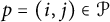
 $p = (i,j)$
, for example, in order to consider the region “inside” or “outside” of p. In this case, we write
 $(p,<_i)$
to indicate that p is directed from edge i to edge j, and
 $(p,<_j)$
for the opposite direction.
We take the convention that all vertices should always be interpreted in terms of the cyclic order on V. So, for any
 $i\in V$
, we will use
 $i+1$
to denote the successor of i in the cyclic order on V. In particular, if
 $V = [n]$
, then all vertices are interpreted modulo n and
 $(n,n+3)$
, for example, means the propagator connecting edges
 $3$
and n.
On both of the last two points, we differ from the standard convention in the physics literature, where propagators are written as ordered pairs
 $(i,j)$
with
 $1 \leq i<j \leq n$
. Furthermore, note that in this paper, we allow for the propagator set
 $\mathcal {P}$
to be empty. This is for mathematical convenience, even though these diagrams do not correspond to tree-level scattering amplitudes. In addition, because
 $\mathcal {P}$
is defined to be a set of pairs, parallel propagators (propagators starting and ending on the same pair of edges) are already excluded from this formulation, but nothing of physical importance is lost as the admissibility restriction(Definition 2.4) would have excluded them on physical grounds.
Definition 2.2 Let
 $W = (\mathcal {P}, V)$
be a Wilson loop diagram.
-
(1) For
 $p = (i,j) \in \mathcal {P}$
, let
$V(p) = \{i, i+1, j, j+1\}$
denote the set of vertices supporting p. For a set of propagators
$P \subseteq \mathcal {P}$
, define to be the vertex support of P.
$$ \begin{align*}V(P) = \bigcup_{p \in P} V(p)\end{align*} $$
-
(2) For
$U \subseteq V$
, the set of propagators supported on U is denoted by Note that a propagator in
$$ \begin{align*}\text{Prop}(U) = \{ p \in \mathcal{P}\ |\ V(p) \cap U \neq \emptyset \}.\end{align*} $$
$\text {Prop}(U)$
does not necessarily have its entire support contained in U.
-
(3) Vertices of W that do not support any propagators are called nonsupporting.





We will see in latter sections that all four vertices supporting a propagator are important in understanding the contribution of that propagator to the objects represented by the diagram. This motivates the following definition of a subdiagram, which can consist of any subset Q of the propagators and any subset U of the vertices of W, but U must contain the support of Q.
Definition 2.3 Let
 $W = (\mathcal {P}, V)$
be a Wilson loop diagram. Then,
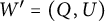 $W' = (Q,U)$
is a subdiagram of W if
 $Q \subseteq \mathcal {P}$
and
 $V(Q) \subseteq U \subseteq V$
.
With these definitions in hand, we can impose some conditions on the density and behavior of the propagators of Wilson loop diagrams.
Definition 2.4 A Wilson loop diagram
 $W = (\mathcal {P}, V)$
is called admissible if the following conditions hold.
-
(1)
$|V| \geq |\mathcal {P}| + 4$
. -
(2) For each nonempty subset of propagators,
$Q \subseteq \mathcal {P}$
, we have
$|V(Q)|\geq |Q| + 3$
. -
(3) There are no crossing propagators. That is, there does not exist
${\{(i,j),(k,l)\} \subseteq \mathcal {P}}$
such that
$i < k < j < l$
.
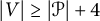




The first condition bounds the total number of propagators in the diagram, whereas the second limits how densely propagators can be fitted into any part of the diagram. The third condition simply requires that propagators are noncrossing.
All three of these conditions arise from the physical interpretation of Wilson loop diagrams. The first condition comes from the fact that these diagrams represent
 $N^k$
MHV interactions, where
 $k +4 <n$
; see, for instance, the explanation in the introduction of [Reference Adamo and Mason2]. The second condition can be derived from the integrals associated to the diagrams (as in [Reference Agarwala and Marin-Amat8, Theorem 1.13]). Note that the second condition prohibits propagators that connect two adjacent edges. In our definition,
 $\mathcal {P}$
is a set, so we may not have two propagators starting and ending on the same pair of edges, but we have lost nothing of physical value by not allowing multiple propagators ending on the same pair of edges, because these would also fail the second condition. The third condition comes from the fact that these Wilson loop diagrams are a representation of planar Feynman diagrams of
 $N=4$
SYM theory. For a description of the relationship between planar Feynman diagram and planar Wilson loops, see the discussion in [Reference Lipstein and Mason26, Section 3].
Note that a subdiagram
 $(Q,U)$
of an admissible Wilson loop diagram need not be admissible itself. It inherits conditions 2 and 3 automatically, but we could have
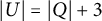 $|U| = |Q| + 3$
. If a Wilson loop diagram satisfies conditions 2 and 3 of Definition 2.4, we call it weakly admissible.
These diagrams correspond to (tree-level) amplitudes of SYM
 $N=4$
theory in twistor space. As such, a diagram associates a real value to n particles, one for each vertex. Each particle is represented as a section of a
 $|\mathcal {P}|$
-vector bundle over twistor space, projected onto a real subspace in a process called bosonization [Reference Eden, Heslop and Mason20, Section 2]. In other words, each Wilson loop diagram defines a functional on external particles. This is represented as an integral
 $I(W)$
, which is the equivalent of a Feynman integral in this setting. This integral is built from two main components: an interaction matrix
 $C(W)$
, and a volume form
 $\Omega (W)$
. These are described next.
A
 $|\mathcal {P}| \times n$
matrix
 $C(W)$
represents the (tree-level) particle interactions. Each row of
 $C(W)$
corresponds to an internal propagator, and each column to an external particle (i.e., a vertex). The matrix
 $C(W)$
is defined as follows:
 $$ \begin{align} C(W)_{p,q} = \begin{cases} x_{p,q} & \text{ if } q \in V(p) \\ 0 & \text{ if } q \not \in V(p) \end{cases} \;. \end{align} $$
The entries
 $x_{p,q}$
are nonzero real variables. Thus, the zero entries in row p correspond to the external particles that the propagator p does not interact with. See Example 2.1 for an example of a diagram W and its associated matrix.
The matrix
 $C(W)$
defines a positroid cell associated to W in the positive Grassmannian
 $\mathbb {G}_{\mathbb {R}, \geq 0}(n, |\mathcal {P}|)$
, which we denote by
 $\Sigma (W)$
[Reference Agarwala and Marin-Amat8, Theorem 3.41]. Marcott [Reference Marcott27, Theorem 8.4] showed that the matrix
 $C(W)$
parametrizes a space whose closure is exactly the closure of
 $\Sigma (W)$
. That is, the space defined by
 $C(W)$
and the cell
 $\Sigma (W)$
agree up to a set of measure
 $0$
. Most of the work in this paper and in the previous paper in the series [Reference Agarwala, Fryer and Yeats6] focuses on characterizing the positroid cell associated to each Wilson loop diagram W.
Note that because there is no ordering on the propagators of W,
 $C(W)$
is only defined up to rearrangement of the rows. When needed, we will impose various different orders on these rows to suit the task at hand. The choice of ordering does not affect
 $\Sigma (W)$
.
One may also interpret the functional
 $I(W)$
as associating a volume to each cell
 $\Sigma (W)$
[Reference Agarwala and Marin-Amat8, Reference Eden, Heslop and Mason20, Reference Heslop and Stewart23], where the volume is determined by the external particles involved. Specifically, the integrand is written in terms of the elements of
 $C(W)$
as
 $$ \begin{align} \Omega(W) = \frac{\prod_{r=1}^{|\mathcal{P}|} \prod_{v \in V(p_r)} \text{d}x_{p_r}}{R(W)} \;, \end{align} $$
multiplied by a
 $\delta $
function that evaluates the matrix
 $C(W)$
on the external particles. The denominator
 $R(W)$
is given in Definition 2.5 below.
The differential form
 $\Omega (W)$
is playing a similar role to that of volume forms in the Amplituhedron literature. For the purposes of this paper, we restrict our attention to
 $\Omega (W)$
only, and ignore the
 $\delta $
function in the integrand of
 $I(W)$
. The interested reader is referred to [Reference Adamo and Mason3, Reference Heslop and Stewart23, Reference Lipstein and Mason26] for more information about the integrand of
 $I(W)$
.
For a fixed number of propagators and particles, the tree-level amplitude of the Wilson loop diagrams is computed as the sum of the
 $I(W)$
for all W of the correct size. By [Reference Adamo, Bullimore, Mason and Skinner1, Reference Arkani-Hamed and Trnka13, Reference Britto, Cachazo, Feng and Witten15], this sum is finite for all sets of external particles, i.e.,
 $$ \begin{align*} \mathcal{A}_{k, n}^{tree} = \sum_{\substack{W = (\mathcal{P}, [n]), \\ |\mathcal{P}| = k}} I(W) <\infty. \end{align*} $$
This would certainly hold if the singularities in the integrands
 $\Omega (W)$
cancel out in the sum. The singularities coming from the zeros of
 $R(W)$
are the spurious poles of the theory, as mentioned in the introduction. The physical theory tells us that the spurious poles should cancel. Specifically, it is conjectured that these poles cancel on the boundaries of the positroid cells
 $\Sigma (W)$
, analogous to the analysis in [Reference Arkani-Hamed and Trnka13]. This has been checked for particular classes of examples (e.g., [Reference Agarwala and Fryer5, Reference Eden, Heslop and Mason20, Reference Heslop and Stewart23]) but has not been proved in general.
With this motivation in mind, in Section 5 of this paper, we study the denominator
 $R(W)$
of
 $\Omega (W)$
. The definition of
 $R(W)$
is as follows.
Definition 2.5 Let
 $W = (\mathcal {P},V)$
be an admissible Wilson loop diagram, and fix an edge e. Let
 $\{p_1 \ldots p_r\}$
be the propagators with one end lying on edge e under a counterclockwise ordering. Define the polynomial
 $$ \begin{align*} R_e = x_{p_1,e+1} \prod_{j= 1}^{r-1} \left((x_{p_j,e} x_{p_{j+1},e+1} - x_{p_{j+1},e} x_{p_{j},e+1} ) \right) x_{p_r,e}\;\end{align*} $$
to be the component of
 $R(W)$
associated to edge e. Note that if
 $r = 1$
(i.e., there is exactly one propagator lying on edge e), then this expression simplifies to
 $R_e = x_{p,e} x_{p,e+1}$
. If
 $r=0$
, set
 $R_e = 1$
. The denominator
 $R(W)$
is defined to be the product of all of the
 $R_e$
, i.e.,
 $$ \begin{align*}R(W) = \prod_{e \in V} R_e.\end{align*} $$
This formulation for the denominator comes from the physics literature; see equation (2) in [Reference Heslop and Stewart23]. In Section 5, we give a geometric meaning to the factors
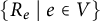 $\{R_e\ |\ e \in V\}$
of
 $R(W)$
. Specifically, given a Grassmann necklace representation of the positroid cell
 $\Sigma (W)$
(see Definition 2.6 and Algorithm 3.5), the
 $R_e$
are exactly the irreducible factors of the minors of
 $C(W)$
defined by the Grassmann necklace. In particular, the question of which minors of
 $C(W)$
contribute to
 $R(W)$
is geometrically determined.
We end this section by computing
 $C(W)$
and
 $R(W)$
for a particular Wilson loop diagram W.
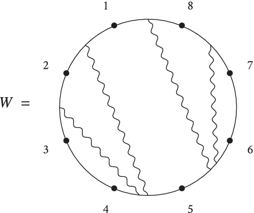
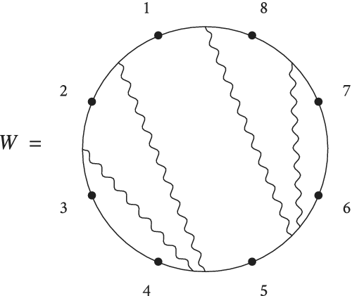
Example 2.1 Consider the admissible Wilson loop diagram
 $$ \begin{align*}W = \big(\{(1,4), (2,4), (5,7), (5,8)\},[8]\big),\end{align*} $$
from Figure 1. Ordering the propagators as listed above, we obtain the associated matrix
 $$ \begin{align*} C(W) = \left( \begin{array}{cccccccc} x_{1,1} & x_{1,2} & 0 & x_{1,4} & x_{1,5} & 0 & 0 & 0 \\ 0 & x_{2,2} & x_{2,3} & x_{2,4} & x_{2,5} & 0 & 0 & 0 \\ 0 & 0 & 0 & 0 & x_{3,5} & x_{3,6} & x_{3,7} & x_{3,8} \\ x_{4,1} & 0 & 0 & 0 & x_{4,5} & x_{4,6} & 0 & x_{4,8} \\ \end{array} \right) \;.\end{align*} $$
The Wilson loop diagram
 $W = \big (\{(1,4), (2,4), (5,7), (5,8)\},[8]\big )$
, which has four propagators and eight vertices.
To calculate
 $R(W)$
, we first compute the polynomials associated to each edge of W:
 $$ \begin{align*} &R_1 = x_{1,1} x_{1, 2}\quad R_2 = x_{2,2} x_{2,3} \quad R_4 = x_{2,5} (x_{2,4}x_{1,5} - x_{2,5}x_{1,4})x_{1,4} \\ &\qquad\qquad R_5 = x_{4,6} (x_{4,5}x_{3,6} - x_{3,5}x_{4,6})x_{3,5} \quad R_7 = x_{3,7} x_{3,8} \quad R_8 = x_{4,8} x_{4,1} \;.\end{align*} $$
All other
 $R_e$
are
 $1$
. Finally, the integrand associated to this Wilson loop diagram (recall equation (2.2)) is
 $$ \begin{align*} &\Omega(W) = \\& \!\frac{\text{d}x_{1,1}\text{d}x_{1,2}\text{d}x_{1,4}\text{d}x_{1,5}\text{d}x_{2,2}\text{d}x_{2,3}\text{d}x_{2,4}\text{d}x_{2,5}\text{d}x_{3,5}\text{d}x_{3,6}\text{d}x_{3,7}\text{d}x_{3,8}\text{d}x_{4,5}\text{d}x_{4,6}\text{d}x_{4,8}\text{d}x_{4,1}}{x_{1,1} x_{1, 2}x_{2,2} x_{2,3}x_{2,5} (x_{2,4}x_{1,5}\!-\!x_{2,5}x_{1,4})x_{1,4}x_{4,6} (x_{4,5}x_{3,6}\!-\!x_{3,5}x_{4,6})x_{3,5}x_{3,7} x_{3,8}x_{4,8} x_{4,1}}. \end{align*} $$
In order to compute the contribution of this diagram to the tree-level scattering amplitude, one needs only to localize the differential form
 $\Omega (W)$
with respect to a delta function that evaluates the matrix
 $C(W)$
at the external momenta.
A reader interested in studying these integrals further is invited to read [Reference Agarwala and Fryer5, Reference Eden, Heslop and Mason20, Reference Heslop and Stewart23] in order to understand the connection to the scattering amplitude of
 $N=4$
SYM theory, the cancellation of spurious poles of specific instances of these integrals as well as explicit amplitude calculations.
2.2 Positroids, Grassmann necklaces, and Le diagrams
We summarize here only the portion of positroid theory that we require in this paper; the interested reader is referred to [Reference Postnikov30, Sections 6 and 16] for more details.
Let
 $\binom {[n]}{k}$
denote the set of all k-subsets of
 $[n]$
.
For our purposes, a positroid isFootnote
1
a matroid M (with ground set
 $[n]$
and set of bases
 $\mathcal {B} \subseteq \binom {[n]}{k}$
) which can be represented by an element of the positive Grassmannian
 $\mathbb {G}_{\mathbb {R}, \geq 0}(k,n)$
. In other words, there exists a full-rank
 $k\times n$
real matrix whose
 $k\times k$
minors are all nonnegative and such that the minor comprised of the columns indexed by elements of J is positive if and only if
 $J \in \mathcal {B}$
.
Postnikov showed in [Reference Postnikov30] that the positroids of
 $\mathbb {G}_{\mathbb {R}, \geq 0}(k,n)$
are indexed by many different collections of objects, each with their own advantages and disadvantages. The two most suited to our purposes are Grassmann necklaces [Reference Postnikov30, Section 16] and Le diagrams [Reference Postnikov30, Section 6], which we discuss. In order to do so, we first need some preliminary definitions.
For each
 $j \in [n]$
, we can define a total order
 $<_j$
on the interval
 $[n]$
by
 $$ \begin{align*} j <_j j+1 <_j \dots <_j n <_j 1 \dots <_j j-1\;.\end{align*} $$
This in turn induces a total order on
 $\binom {[n]}{k}$
, namely the lexicographic order with respect to
 $<_j$
. It also induces a separate partial order
 $\preccurlyeq _{j}$
on
 $\binom {[n]}{k}$
(the Gale order [Reference Gale22]), which is defined as follows: for
 $$ \begin{align*}A = \{a_1 <_j a_2 <_j \dots <_j a_k\} \text{ and } B = \{b_1 <_j b_2 <_j \dots <_j b_k\} \in \binom{[n]}{k},\end{align*} $$
we define
 $$ \begin{align*}A \preccurlyeq_{j} B \text{ if and only if } a_r \leq_j b_r \text{ for all }1 \leq r \leq k.\end{align*} $$
For example, in
 $\binom {[6]}{3}$
, we have
 $\{2,5,6\}\preccurlyeq _{2} \{2,6,1\}$
, but
 $\{2,5,6\}\not \preccurlyeq _{2}\{3,4,6\}$
.
Definition 2.6 A Grassmann necklace of type
 $(k,n)$
is a sequence
 $(I_1, \dots , I_n)$
of n sets
 $I_i \in \binom {[n]}{k}$
such that for each
 $i \in [n]$
, the following statements are true.
-
• If
$i \in I_i$
, then
$I_{i+1} = \big (I_i \backslash \{i\}\big ) \cup \{j\}$
for some
$j \in [n]$
. -
• If
$i \not \in I_i$
, then
$I_{i+1} = I_i$
.




By convention, we set
 $I_{n+1} = I_1$
.
By [Reference Postnikov30, Theorem 17.1], the Grassmann necklaces of type
 $(k,n)$
are in 1–1 correspondence with the positroid cells in
 $\mathbb {G}_{\mathbb {R}, \geq 0}(k,n)$
. Each term
 $I_i$
is simply the minimal (with respect to the
 $<_i$
-lex order) basis of the positroid. A characterization of all bases of the positroid in terms of the Grassmann necklace and the Gale order was given by Oh in [Reference Parke and Taylor29, Theorem 8]: if
 $(I_1, \dots , I_n)$
is the Grassmann necklace associated to a positroid
 $M = ([n],\mathcal {B})$
, then the bases of M are exactly
 $$ \begin{align} \mathcal{B} = \left\{J \in \binom{[n]}{k}\ \Big|\ I_i \preccurlyeq_{i} J \ \ \forall i \in [n]\right\}. \end{align} $$
Thus, the Grassmann necklace is well suited to testing whether a given k-set is a basis for M, and for generating a list of all bases of M.
Definition 2.7 A Le diagram is a Young diagram in which every square contains either a
 $+$
or a
 $0$
, subject to the rule that if a square contains a
 $0$
, then either all squares to its left (in the same row) must also contain a
 $0$
, or all squares above it (in the same column) must also contain a
 $0$
, or both.
By [Reference Postnikov30, Theorem 6.5], the set of all Le diagrams that fit within a
 $k\times (n-k)$
rectangle is in 1–1 correspondence with the positroid cells of
 $\mathbb {G}_{\mathbb {R}, \geq 0}(k,n)$
. Le diagrams are particularly useful for comparing dimensions of positroids, because the dimension of a positroid is equal to the number of
 $+$
squares in its Le diagram [Reference Postnikov30, Theorem 6.5].
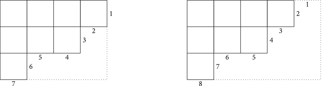
The rows and columns of a Le diagram are labeled as follows: given a Le diagram fitting inside a
 $k\times (n-k)$
box, arrange the numbers
 $1,2, \dots , n$
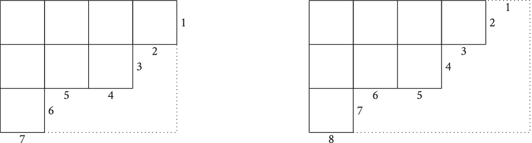
along its southeast border, starting from the top-right corner. See Figure 2 for examples.
Row and column numbering for a Young diagram with
 $k = 3$
,
 $n = 7$
(left), and
 $k = 3$
,
 $n = 8$
(right). The top-left box has coordinates
 $(1,7)$
in the left diagram, and
 $(2,8)$
in the right diagram.
Specifying a k-subset
 $J \subseteq [n]$
therefore uniquely determines the shape of the Le diagram, by taking the elements of J to be the row indices of the diagram.
An algorithm for constructing the Le diagram associated to a Grassmann necklace was given by Agarwala and Fryer in [Reference Agarwala and Fryer4]. Because we will make use of this algorithm in Section 4, we summarize the process here.
Algorithm 2.2 [Reference Agarwala and Fryer4, Algorithm 2]
Let (I 1, …, I n ) be a Grassmann necklace of type (k, n). Within a k × (n − k) square, draw the Young diagram whose rows are labeled by I 1 (as per the convention above).
For each i, 2 ≤ i ≤ n, perform the following steps.
-
• Write
where the inequalities denote the <1 order (subscripts suppressed for clarity).
$$ \begin{align*}I_1 \setminus I_i = \{a_1> a_2 > \dots > a_r\}, \ \ \ I_i \setminus I_1 = \{b_1 < b_2 < \dots < b_r\},\end{align*} $$
-
• For 1 ≤ j ≤ r, place a + in square (a j , b j ) of the diagram. (We will refer to this + as being in the a j → b j position.)

After performing the above, for 2 ≤ i ≤ n, place a 0 in any remaining unfilled boxes.
An algorithm for constructing the Grassmann necklace of a Le diagram also exists; this was given by Oh in [Reference Parke and Taylor29, Section 4]. A method for using the Le diagram to test whether a given k-subset is a basis for the corresponding positroid or not was given by Casteels in [Reference Casteels18].
2.3 Wilson loop diagrams as positroids
Let
 $W = (\mathcal {P},[n])$
be an admissible Wilson loop diagram with k propagators, and
 $C(W)$
the associated matrix defined in equation (2.1). Let
 $M(W)$
be the matroid realized by
 $C(W)$
, i.e., the matroid with ground set
 $[n]$
whose independent sets are exactly those sets
 $V \subseteq [n]$
such that the columns of
 $C(W)$
indexed by V are linearly independent.
In [Reference Agarwala and Marin-Amat8], Agarwala and Marin-Amat showed that
 $M(W)$
can also be read directly from the Wilson loop diagram itself.
Theorem 2.3 [Reference Agarwala and Marin-Amat8, Theorem 3.6]
The independent sets of the matroid
 $M(W)$
associated to an admissible Wilson loop diagram
 $W = (\mathcal {P},[n])$
and realized by
 $C(W)$
are exactly those subsets
 $V \subseteq [n]$
such that there is no subset
 $U \subseteq V$
satisfying
 $|\text {Prop}(U)| < |U|$
.
In other words, the independent sets of
 $M(W)$
correspond to sets of vertices in W in which no subset supports fewer propagators than the vertices it contains.
One useful corollary of this, which we will want to keep in mind later, is the following.
Corollary 2.4 Let
 $W = (\mathcal {P},[n])$
be an admissible Wilson loop diagram, and let
 $M(W)$
be its associated matroid. A subset
 $J \subseteq [n]$
is an independent set of
 $M(W)$
if and only if there exists an injective set map
 $f : J \rightarrow \mathcal {P}$
with the property that for each
 $j\in J$
, we have
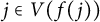 $j \in V(f(j))$
.
Proof This follows as a corollary of the previous theorem by induction in one direction and the pigeonhole principle in the other direction.
Alternatively, we can simply think about the condition of linear independence in the matrix
 $C(W)$
, and so the corollary can also be proved directly by linear algebra and the definition of
 $C(W)$
as follows.
Because the nonzero entries of
 $C(W)$
are independent indeterminates, J is an independent set if and only if there is some choice of
 $|J|$
nonzero entries of
 $C(W)$
, one in each row associated to an element of J and each in different columns. Each entry in
 $C(W)$
identifies a propagator by the row of the entry and a vertex by the column of the entry. The entry is nonzero if and only if the propagator is supported on that vertex. Consequently, take a choice of
 $|J|$
nonzero entries of
 $C(W)$
, one in each row associated to an element of J and each in different columns. Such a choice is equivalent to an assignment of the propagators of J to supporting vertices, so that no two are assigned to the same vertex. Such an assignment of the propagators of J to supporting vertices is exactly a map f as described in the statement, hence proving the result.▪
In particular, this corollary says that a subset J of
 $[n]$
is a basis of
 $M(W)$
if and only if there is a set bijection between J and
 $\mathcal {P}$
with the property that for each
 $j\in J$
, the propagator associated to j under the bijection is supported on vertex j.
By relating the behavior of the propagators in W to the matroidal properties of
 $M(W)$
, Agarwala and Marin-Amat also showed that
 $M(W)$
is a positroid whenever W is admissible [Reference Agarwala and Marin-Amat8, Corollary 3.39].
However, to go from the Wilson loop diagram W to the positroid cell, one had to go through the matroid explicitly realized via
 $C(W)$
, then make a list of all its nonzero
 $k\times k$
minors and extract the Le diagram or Grassmann necklace via the methods described in Section 2.2. In [Reference Agarwala and Fryer5, Section 4], Agarwala and Fryer applied this process in the smallest nontrivial case: admissible Wilson loop diagrams with two propagators on six vertices. Even in this simple case, we see that the mapping from admissible Wilson loop diagrams to positroid cells is neither one-to-one nor onto, and the process described above makes it almost impossible to track the relationship between the original Wilson loop diagram and the resulting positroid.
Our first goal is therefore to find a better method of obtaining the positroid associated to a given Wilson loop diagram; this is the focus of the next section.
Remark 2.5 While this paper primarily approaches proofs from a combinatorial point of view, readers with a background in matroid theory are encouraged to keep the matroidal viewpoint in mind throughout; we expect that the two approaches will be complementary and will build upon each other. See the first paper in this series [Reference Agarwala, Fryer and Yeats6, Section 3] for some related results concerning the positroids of Wilson loop diagrams obtained by viewing them primarily as matroids.
3 Wilson loop diagrams and their Grassmann necklaces
In this section, we will give an algorithm (Algorithm 3.5) to go directly from a Wilson loop diagram to the Grassmann necklace of its positroid.
This is a useful result in and of itself, as it greatly simplifies the process of identifying the positroid associated to a given Wilson loop diagram. We also use it to characterize loops and coloops in the positroid associated to a Wilson loop diagram (Corollary 3.16). The characterization of the coloops, in particular, was not at all clear from the definition of Wilson loop diagrams but is an easy corollary of the algorithm.
Furthermore, the algorithm allows us to see how the Le diagram associated to a Wilson loop diagram changes as one adds propagators in certain positions (Theorem 4.12). Indeed, the techniques we develop in this section to verify that our algorithm produces the correct Grassmann necklace will also be used repeatedly in latter sections to calculate the dimension of the associated positroid cell (Section 4) and to study the structure of the poles of the associated integrand
 $\Omega (W)$
(Section 5).
One of the key insights is that each element of the Grassmann necklace can be viewed as a function from the propagators of the diagram to the vertices in the Grassmann necklace element. This is captured in Definition 3.3, and used throughout the paper.
The flavor of the calculations is similar to [Reference Chavez and Gotti19], as in both our paper and theirs,Footnote 2 the bijections are very explicit with a similar iterative flavor using Le diagrams and Grassmann necklaces related to another class of objects, for us Wilson loop diagrams and for them unit interval orders. For them, as us, the Le diagrams are particularly useful for understanding the dimensions of positroid cells, because the dimension becomes the count of the number of plusses. The ubiquitous Catalan numbers arise for them, as for us in [Reference Agarwala, Fryer and Yeats6]. The specific subclasses of positroids we work with are, however, different. This basic methodology of gaining insight from bijections is very common in combinatorics.
Throughout this section,
 $W = (\mathcal {P},[n])$
is an admissible Wilson loop diagram with k propagators.
3.1 Propagator configurations in admissible Wilson loop diagrams
Before we can describe the algorithm for extracting the Grassmann necklace of
 $M(W)$
from the Wilson loop diagram W, we require some initial results about the behavior of propagators in admissible Wilson loop diagrams.
Definition 3.1 Let
 $W = (\mathcal {P}, [n])$
be a weakly admissible Wilson loop diagram, with
 $p \in \mathcal {P}$
supported on edges i and j. Write
 $(p, <_i)$
to represent the same propagator directed from i to j. Then, the sets of propagators inside and outside
 $(p,<_i)$
are defined to be
 $$ \begin{gather*}\mathcal{P}_{in}(p,<_i) = \{ (k,l) \in \mathcal{P} \ |\ i \leq_i k <_i l \leq_i j \}, \\ \mathcal{P}_{out}(p,<_i) = \mathcal{P}\setminus \mathcal{P}_{in}(p,<_i), \end{gather*} $$
respectively.
Note that we have
 $p\in \mathcal {P}_{in}(p, <_i)$
, and so
 $\mathcal {P}_{in}(p, <_i) = \mathcal {P}_{out}(p, <_j)\cup \{p\}$
.
Example 3.1 Let W be the Wilson loop diagram from Figure 1, reproduced here for convenience.

Let p be the propagator
 $p = (1, 4)$
. Then,
 $(p,<_4)$
indicates that we are viewing p as being directed from 4 to 1, and we have
 $$ \begin{gather*}\mathcal{P}_{in}(p, <_4) = \{(1,4), (5, 8), (5, 7) \};\\ \mathcal{P}_{out}(p, <_4) = \{(2,4) \}. \end{gather*} $$
Definition 3.2 Let
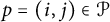 $p = (i,j) \in \mathcal {P}$
be a propagator in W. Define the length of p to be
 $$ \begin{align*}\ell(p) \ =\ \min\big\{|[i+1,j]|,|[j+1,i]|\big\}.\end{align*} $$
In other words,
 $\ell (p)$
is the size of the smaller of the sets of vertices on either side of the propagator p.
Remark 3.2 The following observations about configurations of propagators of short length in a weakly admissibly Wilson loop diagram W are easily verified.
-
(1) If
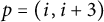
$p = (i,i+3)$
is a propagator of length 3, then the middle vertex
$i+2$
supports at most one propagator. -
(2) If every vertex in W supports at least one propagator, then W admits at least one propagator of length 2. By the same reasoning, if
$p=(i,j)$
is a propagator of W and every vertex in the interval
$[i,j]$
supports at least one propagator, then there is at least one propagator of length
$2$
in
$\mathcal {P}_{in}(p, <_i)$
.


The following lemma establishes certain configurations of propagators that must exist in any admissible diagram with no nonsupporting vertices. We make use of this result in several induction proofs below.
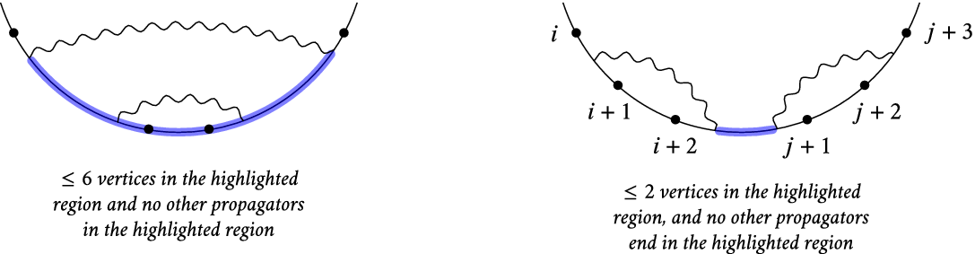
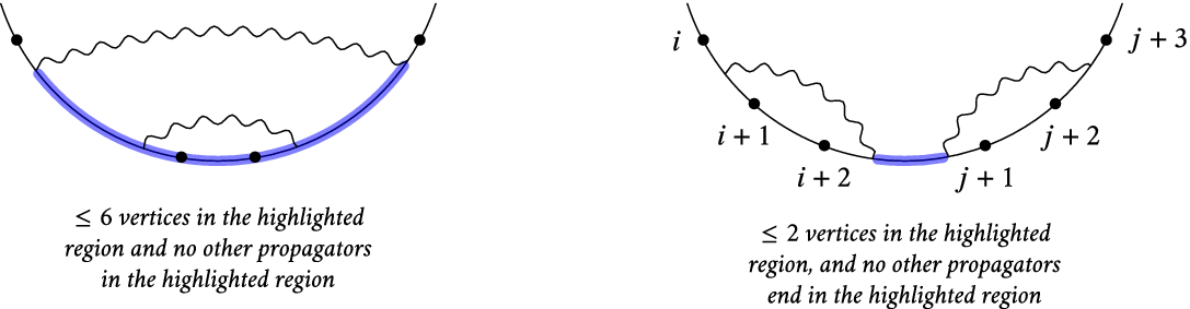
Lemma 3.3 Let W be a weakly admissible Wilson loop diagram with at least five vertices and in which each vertex supports at least one propagator. Then, at least one of the following two conditions holds.
-
(1) The diagram W has a propagator of length at most 6 with a propagator of length 2 on one side of it and nothing else on that side.
-
(2) There exists a pair of propagators of length
$2$
with the property that the first propagator is
$(i, i+2)$
, the second is
$(j, j+2)$
, no other propagator has an end between vertices
$i+2$
and
$j+1$
, and
$j\in \{i+2, i+3, i+4\}$
.



See Figure 3 for an illustration of the two configurations.
The two configurations described in Lemma 3.3; every weakly admissible Wilson loop diagram with no nonsupporting vertices admits at least one example of at least one of these configurations.
Proof Suppose first that W has a propagator of length
 $3$
, say
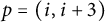 $p=(i, i+3)$
. By Remark 3.2 and the fact that every vertex of W supports at least one propagator, we have that
 $i+2$
supports exactly one propagator, and this propagator must have length 2 by noncrossingness. This gives us an instance of configuration 1 from the statement.
Now, suppose W has no propagators of length
 $3$
.
We will inductively construct sequences of propagators
 $(p_r)$
and
 $(q_r)$
, with
 $\ell (p_r) = 2$
for each r and such that either of the following are true:
-
• the propagator
$p_r$
forms part of configuration 1 or 2 from the statement, at which point the induction terminates, or
-
• there is a propagator
$q_r$
satisfying
$\ell (q_r) \geq 4$
, and
$\{p_1, \ldots , p_r, q_1, \ldots , q_{r-1}\}$
are all on the same side of
$q_r$
.




We can choose the orientation of
 $q_r$
, so that the previous
 $p_i$
and
 $q_i$
are all on the outside of
 $q_r$
, and restrict our attention to the subdiagram
 $(\mathcal {P}_{in}(q_r),[n])$
. By the finiteness of W, this must eventually terminate in one of the desired configurations.
Start by choosing a propagator
 $p_1 = (j_1,j_1+2)$
of length 2 in W (which exists by Remark 3.2). If it is part of one of the configurations we are looking for, we are done, so suppose otherwise.
From our existing assumptions, we know the following facts:
 $p_1$
is not in configuration 2, there are no propagators of length
 $3$
, and every vertex supports at least one propagator. Therefore, there must be a propagator of length at least 4 with one end on edge
 $j_1$
or on edge
 $j_1-1$
or on edge
 $j_1-2$
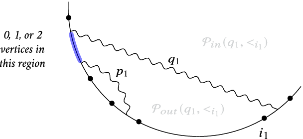
. Let
 $q_1 = (i_1, k_1)$
be this propagator, oriented such that
 $p_1 \in \mathcal {P}_{out}(q_1,<_{i_1})$
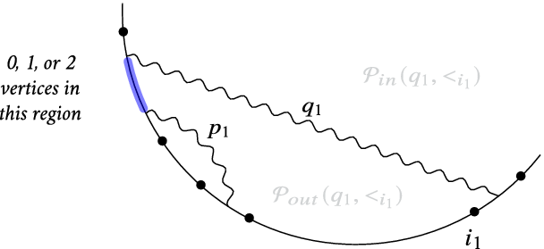
; see Figure 4. This completes the base case.
The base case of the induction in Lemma 3.3.
Now, suppose
 $q_{r} = (i_r, k_r)$
exists by the induction hypothesis and is oriented
 $(q_r, <_{i_r})$
, so that the previous
 $p_i$
and
 $q_i$
are on the outside. For the rest of this proof, we assume this orientation and drop the
 $<_{i_r}$
from the notation.
Let
 $W_r := (\mathcal {P}_{in}(q_r),[n])$
be the subdiagram of W consisting of those propagators inside
 $q_r$
(including
 $q_r$
itself); in particular,
 $W_r$
contains none of the previous
 $p_i$
or
 $q_i$
. By the original hypotheses on W, every vertex in
 $[i_r,k_{r+1}]$
(of which there are at least 4, because
 $\ell (q_r) \geq 4$
) must support at least one propagator. Therefore,
 $W_r$
admits at least one propagator of length 2 (by Remark 3.2) and no propagators of length
 $3$
(by our assumption on W).
Let
 $p_{r+1} = (j_{r+1}, j_{r+1}+2)$
be a propagator of length 2 in
 $W_r$
. If it forms part of configuration 1 or 2, we are done, so assume otherwise.
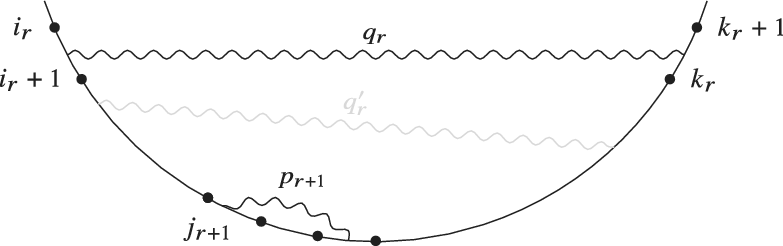
Note that we could replace
 $q_r$
by another propagator
 $q^{\prime }_{r}$
in
 $W_r = (\mathcal {P}_{in}(q_r), [n])$
, as long as
 $p_{r+1}$
and
 $q_r$
are on opposite sides of
 $q_r^{\prime }$
. Such a new
 $q^{\prime }_{r}$
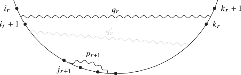
would still satisfy all of the induction hypotheses. (See Figure 5.) Therefore, without loss of generality, we may assume that
 $\mathcal {P}_{in}(q_r)$
does not contain any propagators (other than
 $q_r$
itself) which satisfy the induction hypotheses, i.e., we assume that there are no other propagators with
 $p_{r+1}$
on one side and
 $q_r$
on the other.
We can replace
 $q_r$
with
 $q^{\prime }_r$
as long as
 $q_r$
and
 $p_{r+1}$
are on opposite sides of
 $q^{\prime }_r$
.
There are two cases to consider.
The first case is that
 $i_r \leq j_{r+1} \leq i_r+2$
and
 $k_r-2 \leq j_{r+1}+2 \leq k_{r}$
(so
 $p_{r+1}$
has one end before
 $i_{r} + 3$
and the other after
 $k_{r} - 2$
, i.e., there are at most two vertices between an endpoint of
 $p_{r+1}$
and an endpoint of
 $q_r$
). Because
 $p_{r+1}$
has length 2, it must be that
 $(i_r+3)+1 \geq k_r-2$
, and so
 $q_r$
has length at most 6. By the minimality assumption on
 $q_r$
, no propagator in
 $W_r$
has
 $q_r$
on one side and
 $p_{r+1}$
on the other side. Therefore, any propagator in
 $W_r$
other than
 $q_r$
and
 $p_{r+1}$
must be of the form
 $(i,j)$
with
 $i_r\leq i < j\leq i_r+2$
or
 $k_r-2 \leq i < j\leq k_r$
. Both of these require that
 $(i,j)$
has length 2, and so we have configuration 2 which we have already assumed does not occur. Consequently,
 $W_r$
contains only the two propagators
 $q_r$
and
 $p_{r+1}$
, yielding configuration 1 from the lemma statement and again contradicting our assumption. Therefore, this first case cannot occur.
The second case is that there are at least three vertices between one endpoint of
 $p_{r+1}$
and the nearest endpoint of
 $q_r$
. In other words, at least one of the following four statements are true:
-
•
$i_r+3 \leq j_{r+1}\leq k_r-3$
(one endpoint of
$p_{r+1}$
has at least three vertices between it and the nearest endpoint of
$q_r$
), or -
•
$i_r+3 \leq j_{r+1}+2\leq k_r-3$
(the other endpoint of
$p_{r+1}$
has at least three vertices between it and the nearest endpoint of
$q_r$
), or -
•
$i_r = j_{r+1}$
(
$p_{r+1}$
and
$q_r$
both have an end on edge
$i_r$
), or -
•
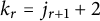
$k_r = j_{r+1} +2$
(
$p_{r+1}$
and
$q_r$
both have an end on edge
$k_r$
).








In other words, at least one end of
 $p_{r+1}$
is supported entirely by vertices in the interval
 $[i_r+3,k_r+2]$
(the first two bullet points) or both ends lie in
 $[i_r, i_r+3]$
(third point) or both ends lie in
 $[k_r-2, k_r+1]$
(fourth point). These situations all behave similarly, and by symmetry, it suffices to only consider the second and third possibilities.
We have
 $j_{r+1}+4 \leq k_r-1$
in both of these cases. In the situation of the second bullet point, this follows directly from the inequality, whereas in the third case, it follows from the fact that
 $\ell (p_{r+1}) = 2$
and
 $\ell (q_r) \geq 4$
. Therefore, the vertex
 $j_{r+1}+4$
is in the interval
 $[i_r, k_r+1]$
but does not support either
 $q_r$
or
 $p_{r+1}$
, and must therefore support some other propagator t. Because
 $p_{r+1}$
is not part of configuration 2 and
 $W_r$
has no propagators of length 3, it follows that
 $\ell (t) \geq 4$
. If
 $q_r$
and
 $p_{r+1}$
were on different sides of t, this would contradict the minimality of
 $q_r$
. Therefore, we can orient t, so that all previous
 $q_i$
and
 $p_i$
belong to
 $\mathcal {P}_{out}(t)$
, and set
 $q_{r+1} = t$
to continue the induction.
The overall result follows by induction.▪
Remark 3.4 In the case that all vertices of an admissible Wilson loop diagram W support at least two propagators, Lemma 3.3 substantially simplifies. By Remark 3.2, W has no propagators of length
 $3$
. Configuration 1 necessarily entails vertices with support
 $1$
as does configuration 2 unless
 $j=i+2$
. So in the case that W has all vertices with support at least 2, W must contain a pair of propagators of length
 $2$
with the property that the first propagator is
 $(i, i+2)$
, the second is
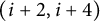 $(i+2, i+4)$
, and no other propagator ends on the edge
 $i+2$
.
3.2 From Wilson loop diagrams to Grassmann necklaces
In this section, we give an algorithm for passing directly from a Wilson loop diagram to its Grassmann necklace. This not only greatly simplifies the previously known process to obtain a positroid cell from a Wilson loop diagram, but also allows us to relate the behavior of the positroid
 $M(W)$
directly to the configuration of propagators in W. In Section 5, we use these results to show that the denominator
 $R(W)$
of the integrand associated to a Wilson loop diagram can be written in terms of the Grassmann necklace of said diagram.
The fact that Algorithm 3.5 does construct the required Grassmann necklace is proved in Theorems 3.14 and 3.15. A worked example of Algorithm 3.5 is given in Example 3.7.
Algorithm 3.5 Let W = (P, [n]) be an admissible Wilson loop diagram. In order to construct the set I i W for i ∈ [n], perform the following steps.
-
(1) Fix a vertex i ∈ [n], the starting vertex. Set j:= i and I i W = ∅.
-
(2) While P≠∅, perform the following steps.
-
(a) Step j for starting vertex i: If Prop(j) = ∅, do nothing. Else, let p ∈Prop(j) be the clockwise-most propagator supported on j. Write I i W = I i W ∪{j}, and delete propagator p from the diagram.
-
(b) Increment j by 1 and repeat from (a).
-
Informally, one starts at i and moves counterclockwise around the vertices of W, at each step removing the clockwise-most propagator supported on that vertex (if it exists). The set
 $I_i^W$
lists the vertices at which a propagator was deleted.
If the algorithm assigns vertex j to propagator p from starting vertex i, we say that p contributes j to
 $I_i^W$
. Notationally, we represent this by allowing the
 $I_i^W$
symbol to represent a function as well as a set, as shown in the below definition.
Definition 3.3 Let
 $W = (\mathcal {P}, [n])$
be an admissible Wilson loop diagram. For each
 $i \in [n]$
, define a function
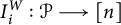 $I_i^W : \mathcal {P} \longrightarrow [n]$
by
 $$ \begin{align*}I_i^W(p) := \text{the vertex label that}\ p\ \text{contributes to}\ I_i\ \text{in Algorithm~3.5,}\end{align*} $$
for each
 $p \in \mathcal {P}$
.
For both
 $I_i^W$
, the set and the function, when the diagram W is clear from context, we drop the superscript and simply write
 $I_i$
.
Remark 3.6 Given
 $W=(\mathcal {P}, [n])$
and
 $i\in [n]$
, the order in which the propagators contribute to the algorithm during the construction of
 $I_i$
defines an order on
 $\mathcal {P}$
.
Because each propagator is removed by the algorithm after it contributes, each propagator contributes exactly once to
 $I_i$
, making the above ordering well defined. Note that different
 $I_*$
impose different orderings on the propagators. Furthermore, we will see below that this ordering respects the ordering of vertices in
 $I_i$
, i.e., if
 $p_j$
occurs before
 $p_l$
in the ordering imposed by
 $I_i$
, then we also have
 $I_i(p_j) <_i I_i(p_l)$
. This will follow directly from Corollary 3.11.
Example 3.7 Consider the admissible Wilson loop diagram:

To construct
 $I_1$
, we start at vertex 1, so we set
 $i=1$
and
 $I_1 = \emptyset $
.
-
• Begin at
$j = 1$
. Because
$\text {Prop}(1) = \{q,r\}$
and r is the clockwise-most of these propagators, r contributes at this step. We let
$I_1 = \{1\}$
and remove propagator r from the diagram. -
• Set
$j = 2$
.
$\text {Prop}(2) = \{p,q\}$
, with q being the clockwise-most of these propagators, so q contributes at this step. We now have
$I_1 = \{1,2\}$
, and propagator q is removed. -
• Set
$j = 3$
.
$\text {Prop}(3) = \{p\}$
, so we have
$I_1 = \{1,2,3\}$
, and we remove propagator p. The only remaining propagator in the diagram is s. -
• Set
$j = 4$
. Because p and q were removed in earlier steps, we now have
$\text {Prop}(4) = \emptyset $
. -
• Set
$j = 5$
.
$\text {Prop}(5) = \{s\}$
, and we have
$I_1 = \{1,2,3,5\}$
.










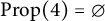



There are no propagators left in the diagram, so the algorithm terminates, and we have
 ${I_1 = \{1,2,3,5\}}$
, which we write more compactly as
 $1235$
.
 $I_1$
viewed as a function is given by
 $$ \begin{align*}I_1: \mathcal{P} \longrightarrow [n] : \quad I_1(r) = 1,\quad I_1(q) = 2, \quad I_1(p) = 3, \quad I_1(s) = 5.\end{align*} $$
Applying the algorithm for all eight starting vertices, we obtain the sets
 $$ \begin{align*}1235, 2356, 3456, 4567, 5671, 6712, 7812, 8123.\end{align*} $$
The reader can easily verify that this sequence of k-sets satisfies the definition of a Grassmann necklace, and can (with significantly more work) also verify that this Grassmann necklace defines the positroid
 $M(W)$
associated to the Wilson loop diagram W above. We will prove this in general shortly.
Remark 3.8 Suppose that we have
 $I_i(p) = a$
for some propagator p and vertex a. Then, p must be the clockwise-most propagator supported on a that has not yet contributed to
 $I_i$
when the algorithm reaches vertex a. In particular, any propagator supported on a that appears later in the ordering given by
 $I_i$
must be inside
 $(p, <_{a-1})$
.
Remark 3.9 The following observation about the local behavior of the algorithm will be very useful in many of the arguments below.
Suppose we are going through the algorithm to construct
 $I_i^W$
for some i, and we are currently at step j of the loop. Consider the diagram
 $W'$
formed by removing from W all propagators that have already contributed to
 $I_i^W$
. (This replicates the behavior of the algorithm, which removes each propagator once it contributes to
 $I_i^W$
.) Now, suppose, for some other diagram V on the same vertex set, we are constructing
 $I_m^V$
for some m, and we are at step j of the loop, for the same j as above. Again, obtain
 $V'$
from V by removing all propagators assigned so far.
With this setup, if we can find a vertex
 $\ell $
occurring after both i and m such that the configuration of propagators ending in the interval
 $[j-1, \ell +1]$
is identical in both
 $W'$
and
 $V'$
, then the vertices contributed to
 $I_i^W$
and
 $I_m^V$
are the same from step j to step
 $\ell $
(inclusive). See Figure 6 for an illustration of this.
 $W'$
and
 $V'$
are locally the same between j and
 $l+1$
, so we will have
 $I_i^W\cap [j,l] = I_m^V\cap [j,l]$
even though
 $p \neq s$
and
 $q \neq t$
. Note that propagators such as r which have both ends inside the region of interest must be identical in both diagrams.

Furthermore, if the propagators of
 $W'$
and
 $V'$
ending in the interval
 $[j-1, \ell +1]$
are also identically labeled, then
 $I_i^W$
and
 $I_m^V$
are the same as functions when restricted to those propagators.
With that in mind, we are ready to begin proving properties of the algorithm. We first show that the algorithm for
 $I_i$
can never reach the final vertex in a propagator’s support (in the
 $<_i$
order) without having already assigned that propagator; in particular, this guarantees that the construction of
 $I_i$
always terminates in fewer than n steps.
Lemma 3.10 Let W be an admissible Wilson loop diagram containing at least one propagator. For any
 $i \in [n]$
and for any
 $p \in \mathcal {P}$
,
 $I_i(p)$
is not maximal (with respect to
 $<_i$
) among the vertices that support p.
Proof Suppose, by way of contradiction, that we have
 $i \in [n]$
and
 $p \in \mathcal {P}$
such that
 $I_i(p)$
is
 $<_i$
-maximal in
 $V(p)$
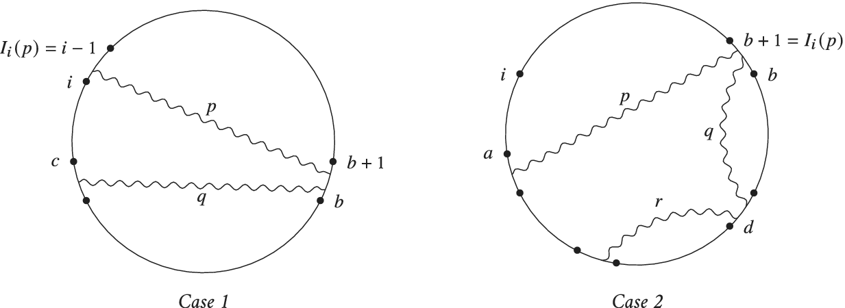
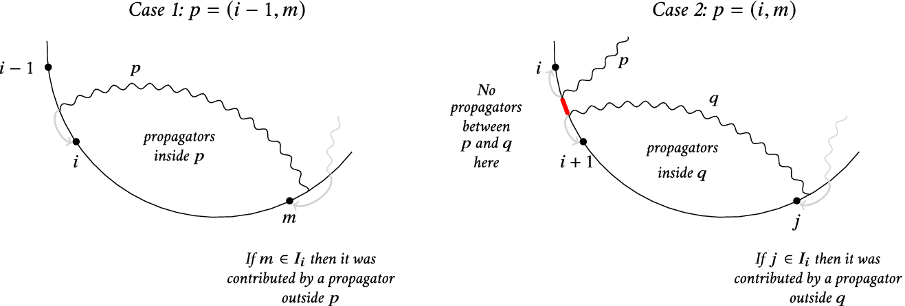
. There are two possibilities, which are illustrated in Figure 7: either
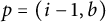 $p = (i-1,b)$
for some b (so i and
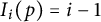 $I_i(p) = i-1$
are the two ends of a single edge), or
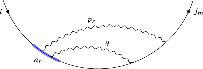
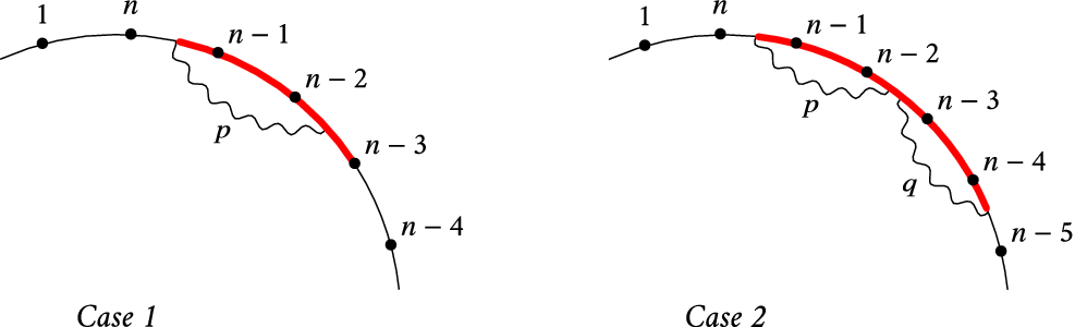
 $p = (a,b)$
with
 $i\leq _i a <_i b$
and
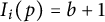 $I_i(p) = b+1$
.
The two types of configuration that would (in theory) allow the propagator p to contribute its
 $<_i$
-maximal support vertex to
 $I_i$
.
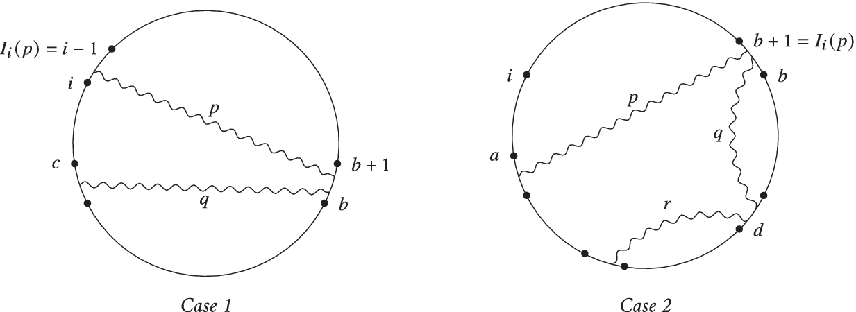
When the first possibility occurs, observe that we must have another propagator
 $q = (c,b)$
with
 $c<_i b$
and
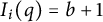 $I_i(q) = b+1$
, because otherwise
 $I_i$
would assign p to
 $b+1$
. Now, q also contributes the
 $<_i$
-maximal vertex in its support to
 $I_i$
and is an instance of the second possibility. Therefore, it suffices to show that no admissible Wilson loop diagram admits the configuration illustrated in Case 2 of Figure 7.
So let
 $p = (a,b)$
with
 $a<_ib$
and
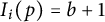 $I_i(p) = b+1$
, and choose p such that
 $\big |[a+1,b]\big |$
is minimal among propagators of W which contribute their last vertex and are in Case 2.
Because
 $I_i(p) \neq b$
, there must exist a propagator q inside
 $(p,<_i)$
with
 $I_i(q) = b$
. The propagator q cannot end on the edge
 $b-1$
, as this would contradict the minimality of p, so we have
 $q = (d,b)$
with
 $a <_i d <_i b$
, and
 $I_i(q) = b$
.
In order for q to remain unassigned until the algorithm reaches vertex b, there must be another propagator r with an end on edge d and
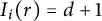 $I_i(r) = d+1$
; the only way this can occur is if r is outside
 $(q,<_i)$
but inside
 $(p,<_i)$
. But now, r contributes its fourth vertex to
 $I_i$
, again contradicting the minimality of p.▪
Corollary 3.11 If W is an admissible Wilson loop diagram with k propagators and n vertices, then Algorithm 3.5 assigns exactly k distinct vertices to each
 $I_i$
in at most n steps.
Proof Fix
 $i \in [n]$
. It follows from the proof of Lemma 3.10 that in applying Algorithm 3.5 to construct the set
 $I_i$
, the algorithm can never reach the fourth vertex of a propagator’s support (ordered with respect to
 $<_i$
) without having already assigned that propagator. Therefore, if the algorithm starts at vertex i, all propagators must have been eliminated by the time it gets to vertex
 $i-1$
, ensuring that the algorithm is completed in at most one full circumnavigation of the diagram and that
 $I_i$
contains exactly k distinct elements.▪
We now reverse our perspective and ask: given a propagator p and a vertex i in the support of p, for which set of starting vertices does the algorithm assign p to i?
Specifically, for each i in the support of p, we define the set
 $$ \begin{align*}J_p^{W}(i) = \{m \in [n] \ | \ I^{W}_m(p) = i \},\end{align*} $$
i.e., the set of starting vertices m such that
 $I_m^{W}$
assigns p to i.
The following lemma establishes that these sets behave in a simple and predictable manner, a fact which we will repeatedly use in subsequent proofs.
Lemma 3.12 Let
 $W = (\mathcal {P},[n])$
be an admissible Wilson loop diagram. For every
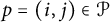 $p = (i,j) \in \mathcal {P}$
, the sets
 $J_p^{W}(i)$
,
 $J_p^{W}(i+1)$
,
 $J_p^{W}(j)$
, and
 $J_p^{W}(j+1)$
are each nonempty cyclic intervals which partition
 $[n]$
and occur in the given cyclic order.
Remark 3.13 Before the proof, let us observe that one of the main ways that the above lemma will be used is in observations like the following. Suppose
 $p=(i,j)$
is a propagator and
 $I_{j+1}(p) = j+1$
. Consider
 $I_{j+2}(p)$
. Because
 $j+1$
is the last vertex in the
 $j+2$
order, p cannot contribute
 $j+1$
to
 $I_{j+2}$
, so the fact that the intervals in the statement of the lemma are nonempty and occur in their cyclic order implies that
 $I_{j+2}(p)=i$
. More generally, we know that whenever a propagator stops contributing a particular vertex, its next contribution must be its cyclically next vertex. This simple observation is surprisingly useful, to the point that the details which appear in the proof of Lemma 3.12 are never needed again. The mere fact of nonempty intervals in the correct order suffices.
Now, we proceed to the proof of Lemma 3.12.
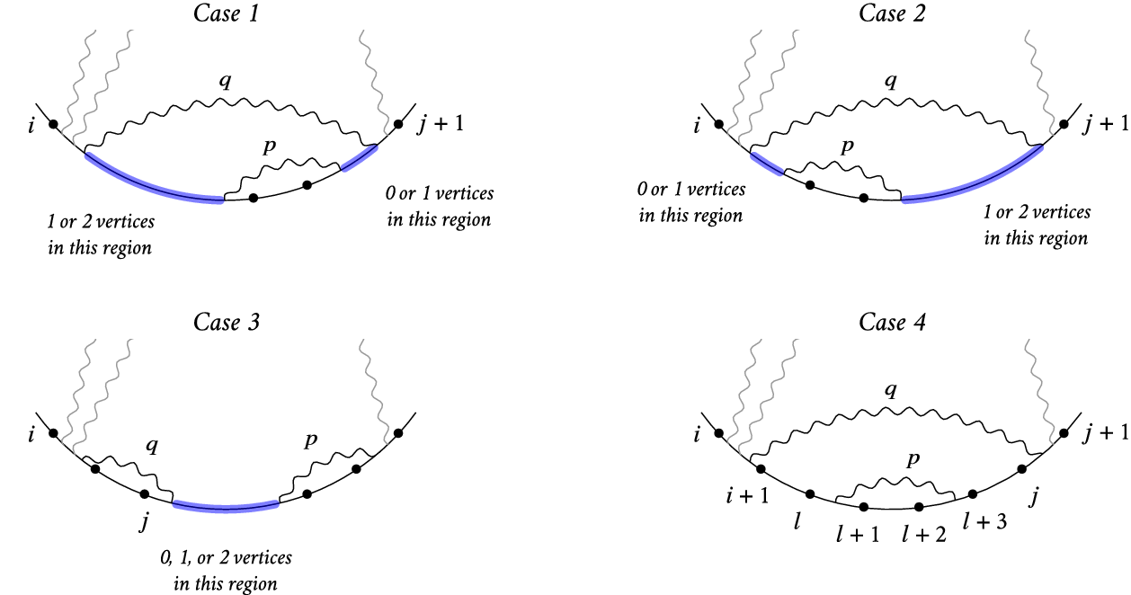
Proof We will prove the result by induction on the number of propagators. If W has one propagator, then the result is immediate. Now, suppose W has more than one propagator. Because nonsupporting vertices have no effect on Algorithm 3.5, it suffices to prove the result for W (possibly weakly admissible) with no nonsupporting vertices. Then, by Lemma 3.3, W has at least one of the four situations illustrated in Figure 8.
Four cases for admissible Wilson loop diagrams with no nonsupporting vertices. The gray half-propagators illustrate where propagators may occur, but are not required to exist.
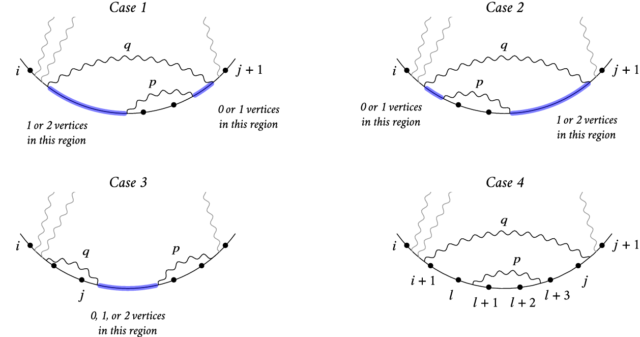
In each of the four cases, when we remove the propagator labeled p, we obtain a diagram which satisfies the statement of the theorem by the induction hypothesis, and contains a propagator
 ${q = (i,j)}$
with no other propagators inside it (with respect to the
 $<_i$
orientation). Note that this region may or may not contain nonsupporting vertices, which we will call
 $l, l+1, \ldots $
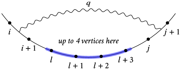
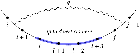
as necessary. Let V be the diagram obtained by removing the propagator p from W (Figure 9). The diagram V is guaranteed to be admissible, because it was formed by removing a propagator from a diagram that was at least weakly admissible.
Diagram V is W with p removed; there are no propagators inside
 $q = (i,j)$
, though there may be up to 4 non-supporting vertices labeled
 $l, l+1, \ldots , l+3$
.
Consider Case 4 of Figure 8 first, as it is the easiest. In this case, the vertices
 ${\{l,l+1,l+2,l+3\}}$
which support p in W are nonsupporting in V, so for every propagator r in V (including q), we have
 $J_r^{V} = J_r^{W}$
; these are nonempty cyclic intervals in the correct order by the induction hypothesis. Furthermore, it is clear from Figure 8 that
 $J_p^{W}(l+a) = \{l+a\}$
for
 $a\in \{1,2,3\}$
and
 $J_p^{W}(l) = [n] \backslash \{l+1, l+2, l+3\}$
. The result therefore holds in this case.
Now, we proceed to consider the first three cases of Figure 8. We first describe
 $J_q^{V}(*)$
, which can be handled identically for all three cases.
In V, there are no propagators inside q by construction, so we see from Figure 9 that
 $$ \begin{align*}l, l+1, \ldots ,j \in J^{V}_q(j) \text{ (if}\ l\ \text{exists)}\ \text{and}\ j+1 \in J^{V}_q(j+1).\end{align*} $$
Note that
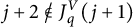 $j+2 \not \in J^{V}_q(j+1)$
by Lemma 3.10, so
 $J^{V}_q(j+1) = \{j+1\}$
, and by the induction hypothesis, we must have
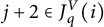 $j+2 \in J^{V}_q(i)$
. Thus, there exist vertices
 $d,e \in [j+2,i+1]$
with
 $d <e$
, such that
 $$ \begin{align} J^{V}_q(i) = [j+2,d-1], \ J^{V}_q(i+1) = [d,e-1], \ J^{V}_q(j) = [e,j], \ J^{V}_q(j+1) = \{j+1\}, \end{align} $$
and all intervals are nonempty.
We now consider what happens as we move from V to each of the three remaining cases for W. We need to consider both
 $J^{W}_p$
and
 $J^{W}_r$
for
 $r \neq p$
, because the addition of p can have a knock-on effect on latter steps in the algorithm.
Cases 1 and 2: These cases behave very similarly except when j or
 $j+1$
are not in the support of p, which can occur in Case 2 only; see below. Consequently, we handle the majority of the proof for these two cases simultaneously. Write
 $p=(m,m+2)$
where
 $m\in \{i, i+1, l\}$
. Let
 $1\leq a\leq 3$
be the number of nonsupporting vertices inside q in V (note that there is at least 1); so these vertices are
 $l, \ldots , l+a-1$
. Note that these vertices are nonsupporting in V but are all in the support of p in W.
We first calculate
 $I^{W}_w$
for a starting vertex
 ${w \in [n]\backslash \{l, l+1, \ldots ,j,j+1\}}$
. Note that p has no effect on other propagators for starting vertices in this range (because p will be the final propagator encountered by the algorithm), so if
 $r \neq p$
, then
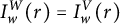 $I_w^W(r) = I_w^V(r)$
. Meanwhile, the value of
 $I^{W}_w(p)$
depends on which step in the algorithm the propagator q contributes a vertex in the diagram V, i.e., on the value of
 $I^{V}_w(q)$
. Thus, if
 $w\in J_q^{V}(i)$
, then
 $$ \begin{align*} I_w^{W}(r) = \begin{cases} \max\{i+1, m\} & \text{if } r=p \\ I_{w}^{V}(r) & \text{if } r\neq p\;, \end{cases} \end{align*} $$
whereas if
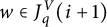 $w\in J_q^{V}(i+1)$
or
 $w\in J_q^{V}(j)$
, then
 $$ \begin{align*} I_w^{W}(r) = \begin{cases} l & \text{if } r=p \\ I_{w}^{V}(r) & \text{if } r\neq p \;. \end{cases} \end{align*} $$
We also need to understand
 $I^{W}_w$
for
 $w \in \{l,l+1,\ldots ,j,j+1\}$
. For the majority of these vertices, we use the following observation: if p is the first propagator to be assigned a value by
 $I_w^{W}$
, then the remainder of
 $I_w^{W}$
proceeds identically to the assignments of
 $I^{V}_{w+1}$
(recall Remark 3.9). Thus, we have, for any
 $0\leq b <a$
,
 $$ \begin{align*} I_{l+b}^{W}(r) = \begin{cases} l+b & \text{if } r=p\\ I_{l+b+1}^{V}(r) & \text{if } r\neq p\;. \end{cases} \end{align*} $$
Similarly, if j is in the support of p, then we have
 $$ \begin{align*} I_j^{W}(r) = \begin{cases} j & \text{if}\ r=p\ \text{and}\ j\ \text{is in the support of}\ p\\ I_{j+1}^{V}(r) & \text{if}\ r\neq p\ \text{and}\ j\ \text{is in the support of}\ p \;. \end{cases} \end{align*} $$
If j is not in the support of p, then we must be in Case 2 of Figure 8 with two vertices in the right-hand region. In this case, if we start the algorithm at j, we need to know whether there will be any unassigned propagators other than p when we reach vertex i, so as to know what p contributes.
Consider the Wilson loop diagram X formed from V by replacing the propagator
 $q = (i,j)$
with
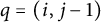 $q = (i, j-1)$
. The diagram X is still admissible, because we have not decreased the support of any set of propagators. It follows from the position of q in X that
 $I_j^X(q) = j$
, and from Lemma 3.10 that
 $I_{j+1}^X(q) \neq j$
. By the induction hypothesis, we must therefore have
 $I_{j+1}^X(q) = i$
. In particular, this means that if we start at
 $j+1$
and assign propagators to vertices according to the algorithm, when we reach vertex i in X, all propagators other than q must have been assigned.
Therefore, if we start at j in W, we first assign q to j, then proceed to assign as in X starting at
 $j+1$
, and hence when we get to i, the only remaining unassigned propagator is p. We obtain
 $$ \begin{align*} I_j^{W}(r) = \begin{cases} m & \text{if}\ r =p\ \text{and}\ j\ \text{is not in the support of}\ p \\ I_{j}^{V}(r) & \text{if}\ r\neq p\ \text{and}\ j\ \text{is not in the support of}\ p\; .\end{cases} \end{align*} $$
This completes the analysis of
 $I_j^W$
. Finally, we consider what happens when we start the algorithm at vertex
 $j+1$
. If
 $j+1$
is in the support of p, then we can argue as above to get
 $$ \begin{align*} I_{j+1}^{W}(r) = \begin{cases} j+1 & \text{if}\ r=p\ \text{and}\ j+1\ \text{is in the support of}\ p\\ I_{j+2}^{V}(r) & \text{if}\ r\neq p\ \text{and}\ j+1\ \text{is in the support of}\ p\;. \end{cases} \end{align*} $$
Now, suppose
 $j+1$
is not in the support of p. If we start at
 $j+1$
, we need to know whether there are any unassigned propagators supported on edge i when we reach vertex i. We already know that
 $J_q^{V}(j+1) = \{j+1\}$
; in particular, this means that q contributes i in
 $I_{j+2}^{V}$
, by the induction hypothesis applied to V. However, the construction of
 $I^{V}_{j+1}$
first assigns q to
 $j+1$
and proceeds identically to
 $I^{V}_{j+2}$
. In particular, if i was assigned in
 $I^{V}_{j+1}$
, then it would not be available to assign to q in
 $I^{V}_{j+2}$
, as all other propagators supported at i in V come before q.
Therefore, p is the only potentially unassigned propagator on edge i when we reach vertex i in the algorithm for
 $I_{j+1}^W$
, and
 $$ \begin{align*} I_{j+1}^{W}(r) = \begin{cases} m & \text{if}\ r=p\ \text{and}\ j+1\ \text{is not in the support of}\ p\\ I_{j+1}^{V}(r) & \text{if}\ r\neq p\ \text{and}\ j+1\ \text{is not in the support of}\ p \;. \end{cases} \end{align*} $$
We can now describe the intervals
 $J^{W}_r(*)$
for Cases 1 and 2 of Figure 8. For
 $r \neq p$
, the intervals are clearly still cyclic and appear in the correct order, and we can assemble the intervals for the
 $J_p^{W}(*)$
as follows. Recall that
 $p = (m,m+2)$
,
 $1 \leq a \leq 3$
, is the number of nonsupporting vertices inside q in V, and these nonsupporting vertices are denoted
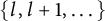 $\{l,l+1, \dots \}$
.
-
• If
$m=l$
, then either
$a=2$
(so
$l+1=m+1$
,
$j=m+2$
, and
$j+1=m+3$
) or
$a=3$
(so
$l+1=m+1$
,
$l+2=m+2$
,
$j=m+3$
, and
$j+1$
is not in the support of p). In both cases, which are nonempty and otherwise as required.
$$ \begin{gather*} J^{W}_p(m) = [m+4, m], \qquad J^{W}_p(m+1) = \{m+1\}, \\ J^{W}_p(m+2) = \{m+2\}, \qquad J^{W}_p(m+3) = \{m+3\}, \end{gather*} $$
-
• If
$m=i+1$
, then checking each of the three different possibilities for a, we likewise get which are nonempty and otherwise as required. Recall that d was defined in equation (3.1).
$$ \begin{gather*} J^{W}_p(m) = [m+4, d-1], \qquad J^{W}_p(m+1) = [d, m+1], \\ J^{W}_p(m+2) = \{m+2\}, \qquad J^{W}_p(m+3) = \{m+3\}, \end{gather*} $$
-
• If
$m=i$
, then
$a=1$
or
$a=2$
; in the former case,
$l=m+2$
,
$j=m+3$
, and
$j+1$
are not in the support of p, so while in the latter,
$$ \begin{gather*} J^{W}_p(m) = \{m+4\}, \qquad J^{W}_p(m+1) = [m+5, d-1], \\ J^{W}_p(m+2) = [d, m+2], \qquad J^{W}_p(m+3) = \{m+3\}, \end{gather*} $$
$l=m+2$
,
$l+1=m+3$
, j, and
$j+1$
are not in the support of p, so which are again as required.
$$ \begin{gather*} J^{W}_p(m) = [m+4, j+1], \qquad J^{W}_p(m+1) = [j+2, d-1], \\ J^{W}_p(m+2) = [d, m+2], \qquad J^{W}_p(m+3) = \{m+3\}, \end{gather*} $$













Case 3: In this case, there are no nonsupporting vertices
 $l, l+1, \ldots $
inside q. Again, write
 ${p=(m, m+2)}$
, where
 $m\in \{j, j+1, j+2\}$
. We proceed as in the previous cases, by computing
 $I^{W}_w$
for vertices w in roughly increasing order of difficulty.
For
 $w \in [n]\backslash \{j+1,m,m+1,m+2,m+3\}$
, if
 $w\in J_q^{V}(i)$
or
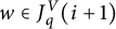 $w\in J_q^{V}(i+1)$
, then
 $$ \begin{align*} I_w^{W}(r) = \begin{cases} m & \text{if } r=p \\ I_{w}^{V}(r) & \text{if } r\neq p \;, \end{cases} \end{align*} $$
whereas if
 $w\in J_q^{V}(j)$
, then
 $$ \begin{align*} I_w^{W}(r) = \begin{cases} \max\{m, j+1\} & \text{if } r=p \\ I_{w}^{V}(r) & \text{if } r\neq p \end{cases} \;. \end{align*} $$
Finally, for
 $j+1$
and the vertices in the support of p, we have
 $$ \begin{align*} I_{j+1}^{W}(r) &= \begin{cases} j+1 & \text{if } r=q\\ j+2 & \text{if } r=p\\ I_{j+3}^{V}(r) & \text{if } r\neq p,q \;, \end{cases} \\ I_m^{W}(r) &= \begin{cases} m & \text{if}\ r=p\ \text{and}\ q\ \text{not supported on}\ m\\ m+1 & \text{if}\ r=p\ \text{and}\ q\ \text{supported on}\ m\\ I_{m}^{V}(r) & \text{if } r\neq p \;, \end{cases} \\ I_{m+1}^{W}(r) & = \begin{cases} m+1 & \text{if}\ r=p\ \text{and}\ q\ \text{not supported on}\ m+1 \\ m+2 & \text{if}\ r=p\ \text{and}\ q\ \text{supported on}\ m+1 \\ I_{m+1}^{V}(r) & \text{if } r\neq p,q \;, \end{cases}\\ I_{m+2}^{W}(r) & = \begin{cases} m+2 & \text{if } r=p \\ I_{m+3}^{V}(r) & \text{if } r\neq p \;, \end{cases}\\ I_{m+3}^{W}(r) & = \begin{cases} m+3 & \text{if } r=p \\ I_{m+4}^{V}(r) & \text{if } r\neq p \;. \end{cases} \end{align*} $$
Note that
 $I_{m+2}^{V}(r) = I_{m+3}^{V}(r)$
for all propagators r in V, and that if
 $j+1\not \in \{m, m+1, m+2, m+3\}$
, then
 $j+2$
and
 $j+3$
are nonsupporting vertices in V, so in that case,
 $I_{j+2}^{V}(r) = I_{j+3}^{V}(r) = I_{j+4}^{V}(r)$
for r in V.
Therefore, once again, we can see that the
 $J_r^{W}(*)$
are cyclic for all
 $r\neq p$
in W. Assembling the intervals for p, we have the following statements.
-
• If
$m=j$
, then Recall that e was defined in equation (3.1).
$$ \begin{gather*}J_p^{W}(m) = [m+4,e-1], \qquad J_p^{W}(m+1) = [e,m], \\ J_p^{W}(m+2) = [m+1,m+2], \qquad J_p^{W}(m+3) = \{m+3\}\;.\end{gather*} $$
-
• If
$m=j+1$
, then
$$ \begin{gather*}J_p^{W}(m) = [m+4,m-1], \qquad J_p^{W}(m+1) = [m,m+1], \\ J_p^{W}(m+2) = \{m+2\}, \qquad J_p^{W}(m+3) = \{m+3\}\;.\end{gather*} $$
-
• If
$m=j+2$
, then
$$ \begin{gather*}J_p^{W}(m) = [m+4,m], \qquad J_p^{W}(m+1) = \{m+1\}, \\ J_p^{W}(m+2) = \{m+2\}, \qquad J_p^{W}(m+3) = \{m+3\}\;.\end{gather*} $$




The result now follows by induction.▪
We are now ready to prove that Algorithm 3.5 gives the Grassmann necklace of the positroid associated to W. We do this in two parts: Theorem 3.14 verifies that the sets
 $(I_1,\dots ,I_n)$
obtained from the algorithm do form a Grassmann necklace, and Theorem 3.15 proves that this Grassmann necklace defines the positroid
 $M(W)$
.
Theorem 3.14 The sequence of k-subsets
 $(I_1,\dots ,I_n)$
obtained by applying Algorithm 3.5 to all vertices of an admissible diagram W is a Grassmann necklace.
Proof For each
 $i \in [n]$
, let
 $I_i$
be the set of vertices assigned to the propagators of W by Algorithm 3.5 with starting vertex i. By Lemma 3.11, we know that
 $|I_i| = k$
for each
 $i \in [n]$
. We prove that
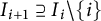 $I_{i+1} \supseteq I_i \backslash \{i\}$
for all
 $i \in [n]$
; this is equivalent to the definition of Grassmann necklace given in Definition 2.6.
Fix n, and suppose, by way of contradiction, that there exists an admissible diagram for which there exists an i with
 $m\in I_i\setminus \{i\}$
and
 $m \not \in I_{i+1}$
. Let W be such a counterexample with the minimal number of propagators.
If
 $i \not \in I_i$
, then there are no propagators supported on i at all. In this case, it is clear that applying Algorithm 3.5 at vertex i and vertex
 $i+1$
produces exactly the same result, i.e.,
 $I_{i+1} = I_i$
, contradicting that W is a counterexample.
Now, suppose that
 $i \in I_i$
. Let p be the propagator which contributes i to
 $I_i$
, that is,
 $I^W_i(p) = i$
; thus, one end of p must lie on either edge
 $i-1$
or edge i. In both cases, let b denote the edge supporting the other end of p, i.e.,
 $p = (i, b)$
or
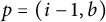 $p = (i-1, b)$
.
Case I: Suppose p has one end on edge
 $i-1$
. By Remark 3.9, the construction of
 $I_i^W$
and
 $I_{i+1}^W$
is locally the same (indeed, locally identical in this case) from vertex
 $i+1$
to
 $b-1$
, so we have
 $I_{i+1}^W \cap [i+1,b-1] = I_{i}^W \cap [i+1,b-1]$
. Note that if
 $b = i+1$
, then this interval is empty, and the equality remains true.
By Lemma 3.12, it must happen that we have
 $I_{i+1}^W(p) = b$
, as otherwise b would never be contributed by p. Consequently, when the construction of
 $I_{i+1}^W$
reaches vertex b, there cannot be any remaining unassigned propagators that are supported on b and clockwise of p (Remark 3.8). It follows that the same must be true when
 $I_i^W$
reaches vertex b, because
 $I_i^W$
and
 $I_{i+1}^W$
behave identically on the interval
 $[i+1,b-1]$
as noted in the previous paragraph.
The previous two paragraphs also imply that
 $m \geq _i b+1$
, because
 $I_{i+1}^W \cap [i+1,b-1] = I_{i}^W \cap [i+1,b-1]$
and
 $b \in I_{i+1}^W$
.
Now, let
 $W' = (\mathcal {P}_{out}(p,<_i), [n])$
, i.e., the diagram obtained from W by removing both p and all propagators inside p. The diagram
 $W'$
has strictly fewer propagators than W did.
Observe that
 $I_i^W$
and
 $I_b^{W'}$
are locally the same from vertex b onward, because by the above observations, the propagators removed from W to create
 $W'$
are exactly those that come first in the ordering defined by
 $I_i^W$
. Similarly,
 $I_{i+1}^W$
and
 $I_{b+1}^{W'}$
are locally the same from
 $b+1$
onward. By Remark 3.9, this yields the equalities
 $$ \begin{align*} I_i^{W} \cap [b,i-1] & = I_b^{W'}, \\ I_{i+1}^{W} \cap [b+1,i-1] & = I_{b+1}^{W'}. \end{align*} $$
Because we have already noted that
 $m \geq _i b+1$
, this implies that
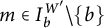 $m\in I_b^{W'}\setminus \{b\}$
and
 $m\not \in I_{b+1}^{W'}$
. This contradicts the minimality of W.
Case II: Suppose p has one end on edge i. Note that by assumption we have
 $I_i(p) = i$
; this means that p must be the clockwise-most propagator lying on edge i, and hence we must have
 $I_{i+1}(p) = i+1$
as well. Observe also that
 $m\geq _i i+2$
, because
 $i+1\in I_{i+1}$
.
Let
 $W'$
be the diagram obtained from W by removing the propagator p. We have
 $$ \begin{align*} I_i^{W} \backslash \{i\} & = I_{i+1}^{W'} \;, \\ I_{i+1}^{W} \backslash \{i+1\} & = I_{i+2}^{W'}\;, \end{align*} $$
because in both cases, the algorithm in
 $W'$
proceeds identically to that in W after assigning p. Because
 $m \neq i+1$
, we have
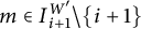 $m\in I_{i+1}^{W'}\setminus \{i+1\}$
, but
 $m\not \in I_{i+2}^{W'}$
, contradicting the minimality of W. This completes the proof.▪
Thus, we have shown that Algorithm 3.5 does produce a Grassmann necklace. Next, we check that it produces the correct one, i.e., the Grassmann necklace that defines
 $M(W)$
.
Theorem 3.15 The Grassmann necklace
 $(I_1 \ldots I_n)$
from Theorem 3.14 is the Grassmann necklace of the positroid
 $M(W)$
.
Proof We have shown in the previous theorem that
 $(I_1,\dots ,I_n)$
is a Grassmann necklace; it remains to check that this Grassmann necklace corresponds to the positroid
 $M(W)$
. Recall from the discussion following Definition 2.6, and equation (2.3) in particular, that it suffices to show the following points.
-
• For each
$i \in [n]$
,
$I_i$
is a basis for
$M(W)$
. -
• If J is lexicographically smaller than
$I_i$
with respect to
$<_i$
(for any
$i \in [n]$
), then J is not a basis for
$M(W)$
.


The first point follows immediately. The algorithm assigns each propagator to a vertex in the support of that propagator, so
 $I_i$
is a basis for
 $M(W)$
by Corollary 2.4.
Now, fix
 $i \in [n]$
, and write
 $I_i = \{a_1 <_i a_2 <_i \dots <_i a_k\}$
. Label the propagators of W according to the ordering imposed by
 $I_i$
, so that
 $I_i(p_{r}) = a_{r}$
for
 $1 \leq r \leq k$
. Define
 $\mathcal {P}_r: = \{p_1,p_2,\dots ,p_r\}$
for each
 $r\geq 0$
, with
 $\mathcal {P}_0 = \emptyset $
.
Let
 $J = \{j_1 <_i j_2<_i \dots <_i j_k\}$
be a k-set, and suppose that
 $J<_i I_i$
in the
 $<_i$
-lexicographic order. Let m be the minimal index such that
 $j_m <_i a_m$
, i.e., the first entry at which J and
 $I_i$
differ. We will show that J must be a dependent set.
If
 $\text {Prop}(j_m) = \emptyset $
, then J is automatically dependent, because the corresponding column of
 $C(W)$
contains only zeros, so suppose henceforth that
 $\text {Prop}(j_m) \neq \emptyset $
.
In order to exhibit a dependent subset of vertices in J, we first define a sequence of sets of propagators by
 $$ \begin{align*}Q_0 = \text{Prop}(j_m), \qquad Q_{l+1} = \text{Prop}(I_i(Q_l))\quad \forall l \geq 0.\end{align*} $$
It is easily verified that this is an increasing chain of sets. Indeed, if
 $q \in Q_l$
, then
 $I_i(q) \in I_i(Q_l)$
, and because
 $I_i(q)$
is one of the vertices that supports q, we must have
 $q \in \text {Prop}(I_i(Q_l)) = Q_{l+1}$
. Because
 $\mathcal {P}$
is finite, the sequence stabilizes in finitely many steps. Let
 $Q := \bigcup _{l \geq 0} Q_l$
be this set of propagators.
We will show that
 $Q \subseteq \mathcal {P}_{m-1}$
, which will imply the theorem by the following argument. If
 $Q \subseteq \mathcal {P}_{m-1}$
, then we have
 $I_i(Q)\subseteq J$
, and hence
 $I_i(Q) \cup \{j_m\} \subseteq J$
as well. Because
 $I_i(Q) \cup \{j_m\}$
only supports the propagators in Q but has
 $|Q|+1$
vertices, it is a dependent set in
 $M(W)$
. Thus, J is also a dependent set, and the Grassmann necklace
 $(I_1,\dots ,I_n)$
constructed from W does indeed define the positroid
 $M(W)$
.
All that remains is to prove
 $Q\subseteq \mathcal {P}_{m-1}$
, which we do by inductively proving
 $Q_l \subseteq \mathcal {P}_{m-1}$
for all
 $l \geq 0$
. The base case
 $Q_0 \subseteq \mathcal {P}_{m-1}$
is immediate; because
 $j_m \not \in I_i$
by construction, there cannot be any unassigned propagators supported on
 $j_m$
when the algorithm reaches that vertex, i.e.,
 ${\text {Prop}(j_m) \subseteq \mathcal {P}_{m-1}}$
.
Now, assume that
 $Q_0,\dots ,Q_{l-1} \subseteq \mathcal {P}_{m-1}$
, and consider
 $Q_{l}$
. If
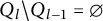 $Q_{l} \setminus Q_{l-1} = \emptyset $
, then we are done, with
 $Q = Q_l$
. Otherwise, let
 $q \in Q_{l} \setminus Q_{l-1}$
. By construction, there is some propagator
 $p_r \in Q_{l-1}$
such that
 $p_r$
and q are both supported on
 $I_i(p_r) = a_r$
. If q is clockwise of
 $p_r$
on vertex
 $a_r$
, then we immediately have
 $q \in \mathcal {P}_{m-1}$
by Remark 3.8. It remains to consider the case that q is counterclockwise of
 $p_r$
at
 $a_r$
.
Note that we cannot have
 $a_r+ 1 = j_m$
when q is counterclockwise of
 $p_r$
, because
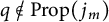 $q \not \in \text {Prop}(j_m)$
by assumption. If the other end of
 $p_r$
(i.e., the end not supported on
 $a_r$
) lies on an edge between
 $a_r$
and
 $j_m$
, then because q is inside
 $p_r$
with respect to
 $<_{a_r-1}$
, we must have
 $V(q) \subseteq [a_r-1,j_m]$
, and hence
 $q \in \mathcal {P}_{m-1}$
by Lemma 3.10; this is illustrated in Figure 10. In particular, if
 $l=1$
, then
 $p_r \in Q_{0} = \text {Prop}(j_m)$
, and we must be in this case.
If q is counterclockwise of
 $p_r$
and the other end of
 $p_r$
lies on an edge between
 $a_r$
and
 $j_m$
, then
 $V(q) \subseteq [a_{r-1},j_m]$
. The vertex
 $a_r$
lies somewhere within the (blue) highlighted region.

If not, then there must be some propagator
 $p_s \in Q_{l-2}$
such that
 $p_r$
and
 $p_s$
are both supported on
 $I_i(p_s) := a_s$
; see Figure 11. Because
 $p_r$
is clockwise of q, and q cannot be supported on
 $I_i(p_s)$
because
 $q \not \in Q_{l-1}$
, it follows that
 $I_i(p_s) <_i I_i(p_r)$
. Therefore, q is inside
 $p_s$
with respect to
 $<_{a_s - 1}$
as well.
If the other end of
 $p_r$
does not lie on an edge between
 $a_r$
and
 $j_m$
, then we must have a propagator
 $p_s \in Q_{l-2}$
in one of the depicted configurations. The (blue) highlighted regions indicate the approximate position of a vertex whose precise position is unknown. Cutoff propagators indicate that the location of the propagator’s other end is unknown; in particular, no meaning should be ascribed to the angle at which these propagators are drawn.

Now, repeat the argument above with
 $p_s$
in place of
 $p_r$
. If the other end of
 $p_s$
lands on an edge between q and
 $j_m$
, then we have
 $q \in \mathcal {P}_{m-1}$
as above; if not, then there exists some
 $p_t \in Q_{l-3}$
with
 $p_s$
supported on
 $I_i(p_t)$
and q on the inside of
 $p_t$
in the
 $a_t-1$
order. Therefore,
 $I_i(p_t) <_i I_i(p_r)$
. Because there are finitely many steps this process can take before reaching
 $Q_0$
, and any
 $p_* \in Q_0 = \text {Prop}(j_m)$
has
 $j_m$
in its support by definition, this argument eventually terminates with the construction of a propagator constraining the positioning of q as required. This completes the induction step, and hence the proof.▪
We have now shown that Algorithm 3.5 associates the correct Grassmann necklace to a Wilson loop diagram. Therefore, we refer to Algorithm 3.5 as the Grassmann necklace algorithm. We close this section with a simple observation about the Grassmann necklaces of positroids associated to Wilson loop diagrams.
In an arbitrary Grassmann necklace, it is possible for an index i to appear in no terms of the Grassmann necklace (a loop) or in all terms of the necklace (a coloop). Using Theorems 3.14 and 3.15, a characterization of the loops and coloops of the Grassmann necklace associated to a Wilson loop diagram follows easily.
Corollary 3.16 Grassmann necklaces coming from admissible Wilson loop diagrams have no coloops. A vertex j is a loop if and only if j supports no propagators.
Proof For any
 $i \in [n]$
,
 $i-1$
is maximal with respect to the
 $<_{i}$
order, and so by Lemma 3.10, there can be no propagator p with
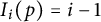 $I_{i}(p) = i-1$
. Thus.
 $i-1 \not \in I_{i}$
, so
 $i-1$
is not a coloop. Because this holds for any
 $i \in [n]$
, the Grassmann necklace admits no coloops.
If
 $j \in [n]$
is a loop, then, in particular, we have
 $j \not \in I_j$
, which can only happen if there are no propagators supported on vertex j. Conversely, if j supports no propagators, then Algorithm 3.5 never assigns a propagator to j and hence
 $j \not \in I_i$
for all
 $i \in [n]$
.▪
4 Dimension of the Wilson loop cells
In continuing to characterize the positroid cells associated to Wilson loop diagrams, our next goal is to show that the dimension of the positroid cell defined by a Wilson loop diagram
 $(\mathcal {P}, [n])$
is
 $3|\mathcal {P}|$
. This is achieved in Theorem 4.12.
Note that the positroid cells associated to the Amplituhedron are of dimension
 $4|\mathcal {P}|$
. In [Reference Agarwala and Marcott7, Section 2], Agarwala and Marcott associated a Deodhar componentFootnote
3
to each Wilson loop diagram, and showed that the dimension of this Deodhar component is the sum of
 $|\mathcal {P}|$
and the dimension of the associated positroid cell. Combining this with Theorem 4.12, we see that the Deodhar component associated to a Wilson loop diagram is
 $4|\mathcal {P}|$
-dimensional, showing that the geometry underlying the Wilson loop diagrams is consistent with the geometry underlying the Amplituhedron. It is worth noting that the Amplituhedron is defined by a projection of a set of
 $4|\mathcal {P}|$
-dimensional positroid cells (i.e., subspaces of
 $\mathbb {G}_{\mathbb {R}, \geq 0}(k,n)$
), while the corresponding
 $4|\mathcal {P}|$
-dimensional cells of the Wilson loop diagram lie in
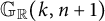 $\mathbb {G}_{\mathbb {R}}(k,n+1)$
. While it is conjectured that the geometry of the Amplituhedron is related to the geometry of the Wilson loop diagrams, in part due to their common physical origin, the
 $3 |\mathcal {P}|$
-dimensional positroid cells defined by the Wilson loop diagrams do not seem to bear any geometric relationship to the
 $4|\mathcal {P}|$
-dimensional positroid cells parametrized by the Amplituhedron.
Marcott in [Reference Marcott27, Theorem 8.4] also gave a proof of the
 $3|\mathcal {P}|$
-dimensionality of
 $M(W)$
, which is much more geometric. However, it is not easy to track the effect of a particular propagator in that proof. By contrast, our approach is much more constructive, and elucidates how each additional propagator contributes to the dimension. By combining Algorithms 3.5 and 2.2 (converting from Wilson loop diagram to Grassmann necklace, and Grassmann necklace to Le diagram, respectively), we explicitly describe the effect of adding another propagator to a Wilson loop diagram in terms of the plusses of the associated Le diagrams. Recall that the dimension of a positroid cell is equal to the number of plusses in its associated Le diagram [Reference Postnikov30, Theorem 6.5]. Thus, understanding the effect of adding another propagator is sufficient to give a recursive proof of the
 $3|\mathcal {P}|$
-dimensionality of the cells.
In order to prove our main theorem of this section, we first require several lemmas.
We begin by relating nonsupporting vertices to columns of zeros in the Le diagram (Lemma 4.1) and verifying that performing dihedral transformations on a Wilson loop diagram does not change the dimension of the associated Le diagram (Lemma 4.2). This allows us to restrict our attention to a particular subset of admissible Wilson loop diagrams (Lemma 4.3) whose Grassmann necklaces can be more easily described.
Lemma 4.1 Let W be an admissible Wilson loop diagram with k propagators, and with a vertex i that supports no propagators. Let V be W with vertex i removed. Then, the Le diagram of W is obtained from the Le diagram of V by inserting an extra column containing all
 $0$
s in position i (i.e., such that the new column has the label i).
Proof By Algorithm 3.5, the Grassmann necklace of W is obtained from the Grassmann necklace of V by duplicating the ith element of the Grassmann necklace of V, and incrementing all indices greater than i by
 $1$
in each Grassmann necklace element. Formally,
 $$ \begin{align*} I_j^{W} = \begin{cases} \{\ell \in I_j^{V} : \ell < i\} \cup \{\ell+1 \in I_j^{V} : \ell \geq i\} & \text{if}\ j\leq i \\ \{\ell \in I_{j-1}^{V} : \ell < i\} \cup \{\ell+1 \in I_{j-1}^{V} : \ell \geq i\} & \text{if}\ j> i. \end{cases} \end{align*} $$
By Corollary 3.16, we know that
 $i \not \in I_1^W$
, and so i must label a horizontal edge on the boundary of the Le diagram of W, i.e., it must be a column label. The shapes of the Le diagram of V and W are the same except for the insertion of this column, because
 $I_1$
is the same for V and W except for the incrementation of the indices greater than or equal to i in the transition from the necklace for V to the necklace for W.▪
Lemma 4.2 If two Wilson loop diagrams differ by a dihedral transformation, then their Le diagrams have same number of plusses.
Proof Recall that the number of plusses in a Le diagram is given by the dimension of the corresponding positroid. By [Reference Postnikov30, Proposition 17.10], the dimension of a positroid M is
 $k(n-k) - A(\pi _M)$
, where
 $A(\pi _M)$
denotes the number of alignments of the decorated permutation
 $\pi _M$
of M. The alignments of a decorated permutation are defined in terms of its chord diagram representation, where an alignment is any pair of noncrossing chords that share the same orientation. See [Reference Postnikov30, Figure 17.1] and the preceding discussion for definitions and more details.
With the help of Algorithm 3.5, it is now easy to trace the effect of a dihedral transformation on a Wilson loop diagram through its Grassmann necklace to its decorated permutation to its chord diagram, and see that dihedral transformations of a Wilson loop diagram W correspond to dihedral transformations of the chord diagram representation of
 $\pi _{M(W)}$
.
Because the number of alignments in a chord diagram is clearly preserved under dihedral transformations, the result follows.▪
Lemma 4.3 Let W be an admissible Wilson loop diagram with
 $k \geq 1$
propagators. Then, there is some dihedral transformation of W such that the resulting diagram
 $W'$
has a propagator p with the following properties.
-
• The propagator
$p = (i, n-1)$
for some i, and p has no propagators inside it with respect to the
$<_i$
ordering. -
• Either the edge i in
$W'$
only supports p, or the edge i in
$W'$
supports exactly one other propagator
$q = (j,i)$
, with no other propagators inside q in the
$<_j$
ordering.
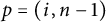


Note that because the first condition tells us that p has nothing inside it, if q exists in the second condition, then
 $j<_ji<_jn-1$
.
Proof Remove all vertices of W which do not support any propagators to get a weakly admissible Wilson loop diagram V. Lemma 3.3 applied to V gives a length 2 propagator p in V for which either no other propagator is supported on one of the supporting edges of p or there is a second length 2 propagator which is the only other propagator supported on one of the supporting edges of p. (Figure 8 shows the possible configurations arising from Lemma 3.3, and the reader can easily check that, in each case, p must be in one of the two situations described above.)
We can now make a dihedral transformation of V to obtain a diagram satisfying the statement of the lemma with p and q both of length 2. Restoring the vertices which do not support any propagators, we obtain a dihedral transformation
 $W'$
of W as desired (with potentially longer lengths for p and q).▪
Combining Lemmas 4.1–4.3, it therefore suffices to study the Le diagrams of weakly admissible Wilson loop diagrams with no nonsupporting vertices and admitting one of the configurations described in Lemma 4.3, with propagators
 $p = (n-3, n-1)$
and
 $q= (n-5, n-3)$
(if q exists) both of length 2. See Figure 12 for an illustration of the two possibilities.
The two cases for W and p following Lemma 4.3. No other propagators can end in the bolded (red) sections. Other segments may have additional propagators ending in them.

With the above restrictions in place, the next few lemmas describe how the Grassmann necklaces (Lemma 4.4) and the Le diagrams (Lemmas 4.6 to Lemma 4.11) change upon the removal of p from the Wilson loop diagram. This gives us the inductive lever we need to prove the main theorem (Theorem 4.12).
Lemma 4.4 Let W be an admissible Wilson loop diagram with
 $k\geq 1$
propagators, and suppose W admits one of the configurations described in Lemma 4.3, with p and q (if q exists) both of length 2. Let V be W with p removed. We can express
 $I_*^W$
in terms of
 $I_*^V$
as indicated below. If
 $k \in \{1, n-1, n-2, n\}$
,
 $$ \begin{align*} I_1^{W} & = I_1^{V} \cup \{n-3\}, \\ I_n^{W} & = I_1^{V} \cup \{n\}, \\ I_{n-1}^{W} & = I_n^{V} \cup \{n-1\}, \\ I_{n-2}^{W} & = \begin{cases} I_{n-2}^{V}\cup \{n-2\} & \text{if}\ n-2\not\in I_{n-2}^{V} \\ I_{n-2}^{V}\cup \{n-1\} & \text{if}\ n-2\in I_{n-2}^{V}, n-1\not\in I_{n-2}^{V} \\ (I_{n}^{V} \setminus \{n-5\})\cup \{n-1,n-2\} & \text{if}\ n-1, n-2\in I_{n-2}^{V} \end{cases} \;. \end{align*} $$
For all other k, i.e.,
 $1<k<n-2$
,
 $$ \begin{align*} I_{k}^{W} & = \begin{cases} I_k^{V}\cup \{n-3\} & \qquad \qquad \qquad \qquad \text{if}\ n-3 \not\in I_k^{V}\\ I_k^{V}\cup\{n-2\} & \qquad \qquad \qquad \qquad \text{if}\ n-3\in I_k^{V} \;. \end{cases} \end{align*} $$
Proof The two possible cases for W are illustrated in Figure 12.
We begin with
 $I_1$
, and first observe that by Remark 3.13, we must have
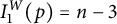 $I_1^W(p) = n-3$
. Because p is the final propagator to be assigned by
 $I_1^W$
, it follows that
 $I_1^W$
and
 $I_1^V$
behaved identically on all earlier propagators (recall Remark 3.9 about locally identical propagator configurations), which implies, in particular, that
 $n-3 \not \in I_1^V$
. Thus,
 $I_1^W = I_1^V\cup \{n-3\}$
.
We note for future reference that the arguments of the previous two paragraphs also imply that
 $n-2$
,
 $n-1$
, and n are not in
 $I_1^V$
.
Next, consider
 $I_n^{W}$
. From Figure 12, we see that in both cases, we have
 $I_n^{W}(p) = n$
. Thus, from vertex 1 onward, the unassigned propagators are exactly those that appear in V. Therefore, the algorithm continues as in
 $I_1^{V}$
, i.e., we have
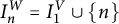 $I_n^{W} = I_1^{V} \cup \{n\}$
. By a similar argument, we must have
 $I_{n-1}^{W} = I_n^{V} \cup \{n-1\}$
.
Now, consider
 $I_{n-2}^{W}$
. If
 $n-2\not \in I_{n-2}^{V}$
, then the vertex
 $n-2$
is nonsupporting (see also Corollary 3.16). Thus, we are in Case 1, with
 ${I_{n-2}^W(p) = n-2}$
, and this assignment of p does not affect the rest of the construction of
 $I_{n-2}^{V}$
, so we obtain
 ${I_{n-2}^{W} = I_{n-2}^{V}\cup \{n-2\}}$
as above.
On the other hand, if
 $n-2\in I_{n-2}^{V}$
, then we must be in Case 2 of Figure 12, and we must have
 ${I_{n-2}^V(q) = I_{n-2}^W(q) = n-2}$
, because q is always the clockwise-most propagator supported on vertex
 $n-2$
. If
 $n-1 \not \in I_{n-2}^{V}$
, then
 $I_{n-2}^W(p) = n-1$
, and the algorithm proceeds identically to
 $I_{n-2}^{V}$
for the remainder of its steps; thus,
 $I_{n-2}^{W} = I_{n-2}^{V}\cup \{n-1\}$
in this case.
Finally, if
 $n-2$
and
 $ n-1$
are in
 $I_{n-2}^{V}$
, then
 $I_{n-2}^W(q) = n-2$
and
 $I_{n-2}^W(p) = n-1$
as above, but some other propagator must have contributed
 $n-1$
to
 $I_{n-2}^{V}$
, so we cannot use the same argument as above. When, in the algorithm, the construction of
 $I_{n-2}^W$
reaches vertex n, only the propagators p and q have contributed; thus, we proceed as in the construction of
 $I_n^{V}$
but without propagator q by Remark 3.9. By Lemma 3.12, we know that
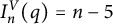 $I_n^V(q) = n-5$
, and from Remark 3.8, we see that the only way this could occur is if q was the last to contribute to
 $I_{n-2}^V$
. Therefore,
 $I_{n-2}^{W} = (I_{n}^{V} \setminus \{n-5\}) \cup \{n-1, n-2\}$
in this case. This completes all cases for
 $I_{n-2}^{W}$
.
The arguments for
 $I_k^{W}$
(
 $1< k < n-2$
) proceed analogously to those of
 $I_{n-2}^{W}$
, with one simplification: we cannot have both
 $n-3$
and
 $n-2$
in
 $I_k^{V}$
, because q is the only propagator that could be assigned to either of them, and it cannot be assigned to both.
This covers all cases and hence completes the proof.▪
The next several lemmas assume V and W to be as above. These lemmas discuss how the shape of the Le diagram changes from V to W and how the plusses in V shift to become plusses in W. In particular, the Le diagram for W has an extra row, labeled by
 $n-3$
, with three columns (see Figure 13 and Lemma 4.6). This last row contains three (new) plusses. All other plusses in the Le diagram of V shift in a predictable manner to become plusses in the Le diagram of W; this is described in Lemma 4.7 to Theorem 4.12.
Le diagrams for V (left) and W (right).

Remark 4.5 To avoid wordiness, we will refer to the row indexed by i in the Le diagram as row i or the i row, and similarly for columns. Note that the i row in this sense is not the ith row, because the indexing for Le diagrams does not label the rows sequentially starting at
 $1$
, and so to avoid confusion, we will not refer to the ith row.
We proceed to address the cases laid out in Lemma 4.4, getting the shape of the Le diagram of W from the relation
 $I_1^W= I_1^V \cup \{n-3\}$
.
Lemma 4.6 Let V and W be as in Lemma 4.4. The shape of the Le diagram of V can be built from left to right of the following blocks: a rectangle which is three columns wide, one more column of the same height, and a partition shape with at most as many rows as the rectangle. The shape of the Le diagram of W can be built from left to right of the following blocks: a rectangle with three columns and one more row than the first rectangle of V, and the same partition shape as in V.
Proof See Figure 13 for an illustration of the shapes described in the statement of the lemma.
Recall that
 $I_1$
determines the shape of the Le diagram. Specifically, the elements of
 $I_1$
label the rows of the diagram, working from top right to bottom left. By the arguments in Lemma 4.4, we know that none of n,
 $n-1$
,
 $n-2$
, and
 $n-3$
are in
 $I_1^{V}$
. These are the leftmost four columns of the diagram for V. From Lemma 4.4, we know that
 $I_1^{W} = I_1^{V}\cup \{n-3\}$
. Therefore, the right-hand boundary of the shape of V is the same as the right-hand boundary of the shape of W except that W has one additional row of three boxes, while V has an additional column in the
 $n-3$
position; that is, an extra column fourth from the left.▪
As illustrated in Figure 13, the pieces of the Le diagrams of V and W will be called
 $\mathcal {A}$
and
 $\mathcal {B}$
, respectively, in what follows. Explicitly,
 $\mathcal {B}$
is the set of columns with labels
 $v < n-3$
, and
 $\mathcal {A}$
is the set of columns labeled by n,
 $n-1$
, and
 $n-2$
in V. In W, we see that
 $\mathcal {A}$
consists of these same three columns, but does not include the last row. Over the course of the next few lemmas, we will prove that the plusses in the
 $\mathcal {B}$
parts of each diagram are identical, and that the relationship between the plusses in the two
 $\mathcal {A}$
regions can be described explicitly.
We do this by applying Algorithm 2.2, which constructs the Le diagram associated to the Grassmann necklaces of V and W. As described in Section 2.2, if Algorithm 2.2 places a
 $+$
in the box with row index i and column index j, we say that this plus is in the
 $i \rightarrow j$
position, and refer to it as the plus defined by “the (hook) path from i to j.” Note that the collection of paths contributed by a single Grassmann necklace term must be noncrossing. This follows immediately from the Le condition.
Lemma 4.7 Let V and W be as in Lemma 4.4. Then,
 $I_n^W$
yields an
 $(n-3)\rightarrow n$
plus, and
 $I_{n-1}^W$
yields an
 $(n-3)\rightarrow (n-1)$
plus along with any plusses yielded by
 $I_n^V$
.
Proof By Lemma 4.4, we have
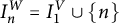 $I_n^{W}= I_1^{V} \cup \{n\}$
and
 $I_1^{W} = I_1^{V} \cup \{n-3\}$
. Thus,
 $$ \begin{align*}I_1^{W} \setminus I_n^{W} = \{n-3\}, \qquad \qquad I_n^{W} \setminus I_1^{W} = \{n\},\end{align*} $$
and so by Algorithm 2.2, we have a plus in the
 $(n-3) \rightarrow n$
position, i.e., in the leftmost box of the bottom row.
Furthermore, by Lemma 4.4, we have
 $I_{n-1}^{W} = I_n^{V} \cup \{n-1\}$
. Recall from the proof of Lemma 4.4 that none of
 $n-3,\;n-2,\;n-1$
, or n are in
 $I_1^V$
; therefore,
 $$ \begin{align*} I_1^W\setminus I_{n-1}^W = (I_1^V \setminus I_n^V) \cup\{n-3\}, \end{align*} $$
and
 $n-3$
is maximal in this set. Similarly,
 $$ \begin{align*}I_{n-1}^W \setminus I_1^W = (I_n^V \setminus I_1^V) \cup \{n-1\}. \end{align*} $$
Moreover,
 $(I_n^V \setminus I_1^V) \cup \{n-1\}\subseteq \{n-1,n\}$
from the definition of Grassmann necklace, and so, in particular,
 $n-1$
is minimal in this set. Thus, Algorithm 2.2 yields a plus in the
 $(n-3) \rightarrow (n-1)$
position (i.e., the second box in the bottom row of the Le diagram of W) along with any plusses yielded by
 $I_n^V$
.▪
We next consider the plusses contributed to the Le diagram of W by
 $I_{n-2}^W$
. Lemma 4.4 lists three possibilities for
 $I_{n-2}^W$
, but the following observation shows that we need to only consider two of these cases.
Remark 4.8 Consider the case when
 $n-2 \in I_{n-2}^V$
but
 $n-1 \not \in I_{n-2}^V$
. This case can only occur if our W is in Case 2 of Figure 12 and
 $n-1$
supports no propagators other than p. In this situation, apply the dihedral transformation that reflects W along the line perpendicular to the
 $(n-2)$
th edge, so that p is unchanged, but
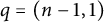 $q = (n-1,1)$
in the new diagram. The new diagram is an example of Case 1, i.e., it satisfies
 $n-2 \not \in I_{n-2}^V$
. Therefore, we do not need to separately consider the case where
 $n-2\in I_{n-2}^V$
but
 $n-1\not \in I_{n-2}^V$
, as it will be subsumed into Case 1 in the main theorem.
We can now describe the plusses contributed by
 $I_{n-2}^W$
in the remaining two cases: when
 $n-2 \not \in I_{n-2}^V$
, and when both
 $n-2$
and
 $n-1$
are not in
 $I_{n-2}^V$
.
Lemma 4.9 Let V and W be as in Lemma 4.4, and suppose that
 $n-2 \not \in I_{n-2}^{V}$
. Then,
 $I_{n-2}^{W}$
contributes all of the same plusses as
 $I_{n-1}^{V}$
(which is the same as
 $I_{n-2}^{V}$
) along with a new
 ${(n-3)\rightarrow (n-2)}$
plus.
Proof If
 $n-2\not \in I_{n-2}^{V}$
, then
 $I_{n-1}^{V}=I_{n-2}^{V}$
by definition, and by Lemma 4.4, we have the equality
 ${I_{n-2}^{W} = I_{n-1}^{V} \cup \{n-2\}}$
. Note that
 $n-3\not \in I_{n-2}^{V}$
by Lemma 3.10. Therefore, the plusses contributed by
 $I_{n-2}^{W}$
are exactly the plusses from
 $I_{n-1}^{V}$
along with the
 $(n-3)\rightarrow (n-2)$
plus. This gives the statement of the lemma.▪
Next, we need an observation about how the Grassmann necklace for V changes over the indices near n under the hypotheses that
 $n-2, n-1\in I_{n-2}^V$
.
Specifically, with V and W as in Lemma 4.4 and with
 $n-2, n-1\in I_{n-2}^V$
(so we are necessarily in Case 2 and
 $n-1$
supports at least one additional propagator), we have
 $$ \begin{align} I_{n-3}^{V} \xrightarrow[\substack{n-3\text{ out}\\n-2\text{ in}}]{} I_{n-2}^{V} \xrightarrow[\substack{n-2\text{ out}\\n-5\text{ in}}]{} I_{n-1}^{V} \xrightarrow[\substack{n-1\text{ out}\\ u \text{ in}}]{} I_{n}^{V} \xrightarrow[\substack{n \text{ out}\\v \text{ in}}]{} I_1^{V} \;, \end{align} $$
where u and v are two vertices. We will derive some properties of u and v below.
The first two transitions follow by the cyclic intervals property highlighted in Remark 3.13 along with the fact that
 $n-3$
is a supporting vertex in V. The third transition follows from the definition of Grassmann necklaces and the fact that
 $n-1\in I_{n-2}^V$
by hypothesis, whereas the final transition follows from the fact that
 $n-1$
supports an additional propagator, so we are guaranteed
 $n \in I_n^V$
.
Note that neither u nor v can be
 $n-1$
,
 $n-2$
, or
 $n-3$
, because as noted in Lemma 4.4, these elements do not belong to
 $I_1^V$
and
 $I_n^V = (I_1^V\setminus \{v\}) \cup \{n\}$
. However, u could be n.
Furthermore, u cannot be
 $n-4$
, for the following reason. By Remark 3.13, we know that
 ${I_{n-1}^W(q) = n-5}$
, leaving no propagators supported on
 $n-4$
for
 $I_{n-1}^W$
to assign. Thus,
 $n-4 \not \in I_{n-1}^W$
. Because
 ${I_{n-1}^W = I_n^V\cup \{n-1\}}$
by Lemma 4.4, we cannot have
 $n-4$
in
 $I_n^V$
either.
However, it is important to observe that v could be
 $n-4$
, as we see in the next result.
Lemma 4.10 Let V and W be as in Lemma 4.4, and suppose that
 $n-2,n-1 \in I_{n-2}^{V}$
. Let c be the largest element of
 $I_1^V$
. Then, the following statements are true.
-
(1) If
$n-4\in I_1^V\setminus I_n^V$
, then
$c=n-4$
. Otherwise,
$c=n-5$
otherwise. If
$c = n-4$
, then we have
$v = n-4$
in equation (4.1). -
(2) The function
$I_{n-3}^W$
contributes the same plusses as
$I_{n-3}^V$
, except that the plus in column
$n-3$
(which necessarily exists) is shifted one square left into column
$n-2$
. -
(3) In the Le diagram of V,
$I_{n-2}^{V}$
contributes a
$(c)\rightarrow (n-2)$
plus, and no other term in the Grassmann necklace of V gives a plus in this column. All other plusses from
$I_{n-2}^{V}$
were already contributed by
$I_{n-3}^V$
. -
(4) The function
$I_{n-2}^W$
contributes an
$(n-3) \rightarrow (n-2)$
plus, a
$(c) \rightarrow (n-1)$
plus, and one other plus. If
$c = n-5$
, then this third plus is the one contributed by
$I_n^V$
, whereas if
$c = n-4$
, then the third plus is
$(n-5) \rightarrow n$
. -
(5) If
$c = n-4$
, then
$I_{n-1}^V$
contributes an
$(n-4) \rightarrow (n-1)$
plus; all other plusses contributed by
$I_{n-1}^V$
were already contributed by
$I_{n-3}^V$
, regardless of the value of c. -
(6) The Grassmann necklace of V contributes a
$(c)\rightarrow (n-1)$
plus if and only if
$c = n-4$
. No term in the Grassmann necklace of V contributes an
$(n-5) \rightarrow n$
plus.
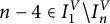















Proof
-
(1) As in Lemma 4.4, we have that none of
$n,\; n-1, \; n-2$
, and
$n-3$
are in
$I_1^V$
, which implies the first part of the claim. The second part is a consequence of the discussion following equation (4.1), which shows that
$n-4 \not \in I_n^V$
. -
(2) By Lemma 4.4, we have that
$I_{n-3}^W = I_{n-3}^V \cup \{n-2\}$
, so
$I_{1}^W \setminus I_{n-3}^W = I_1^V \setminus I_{n-3}^V$
and
$I_{n-3}^W \setminus I_1^W$
is obtained from
$I_{n-3}^V \setminus I_{1}^V$
by replacing the
$n-3$
with
$n-2$
. -
(3) From equation (4.1), the pair of sets
$(I_{n-2}^V\setminus I_1^V, I_1^V\setminus I_{n-2}^V)$
is either
$(\{n-2, n-1, n\}, \{n-5, u, v\})$
(if
$n \in I_{n-2}^V$
) or
$(\{n-2, n-1\}, \{n-5, v\})$
(if
$n \not \in I_{n-2}^V$
, i.e.,
$u = n$
).Recall that we cannot have
$u = n-4$
(because
$n-4 \notin I_n^V$
), so either
$u = n$
or
$u < n-5$
, and either way
$n-2$
is minimal in
$I_{n-2}^V\setminus I_1^V$
and c is maximal in
$I_1^V \setminus I_{n-2}^V$
, yielding a
$(c) \rightarrow (n-2)$
plus.Because
$I_{n-2}^V$
is the only term in the Grassmann necklace for V that contains
$n-2$
, no other term can contribute a plus in column
$n-2$
. In addition, because
$I_{n-2}^V$
only differs from
$I_{n-3}^V$
in that the
$n-3$
was replaced by an
$n-2$
, all other plusses must agree with those contributed by
$I_{n-3}^V$
. -
(4) By Lemma 4.4, we have
$I_1^W = I_1^V\cup \{n-3\}$
and
$I_{n-2}^W = (I_n^V \setminus \{n-5\}) \cup \{n-1,n-2\}$
. By equation (4.1), we have
$n-5 \in I_1^V$
, and by the following discussion, we have that none of
$n-1,\;n-2$
, and
$n-3$
are not in either
$I_n^V$
or
$I_1^V$
. It follows that the symmetric difference of
$I_1^W$
and
$I_{n-2}^W$
is As per the discussion following equation (4.1) above, we must also have
$$ \begin{gather*} I_1^W \setminus I_{n-2}^W = (I_1^V\setminus I_n^V) \cup \{n-3, n-5\}, \\ I_{n-2}^W \setminus I_1^W = (I_n^V\setminus I_1^V) \cup \{n-1, n-2\}. \end{gather*} $$
$I_n^V\setminus I_1^V = \{n\}$
and
${I_1^V\setminus I_n^V = \{v\}}$
. If
$c = n-5$
, then the path
$v \rightarrow n$
from
$I_n^V$
does not intersect with the paths from
$\{n-3, n-5\}$
to
$\{n-2, n-1\}$
, and we obtain the plusses as stated.
Now, suppose
$c = v= n-4$
; in this case,
$I_{n-2}^W$
contributes plusses defined by the noncrossing paths starting from
$\{n-3, n-4, n-5\}$
and ending at
$\{n, n-1, n-2\}$
, namely the plusses in positions
$(n-3)\rightarrow (n-2)$
,
$(n-4)\rightarrow (n-1)$
, and
$(n-5)\rightarrow (n)$
. -
(5) Combining equation (4.1) with point 3 of this proof, the pair
$(I_{n-1}^V \setminus I_1^V, I_1^V \setminus I_{n-1}^V)$
is either
$(\{n-1, n\}, \{u, v\})$
or
$(\{n-1\}, \{v\})$
. Per point 1, we have
$c = n-4$
if and only if
$v = n -4$
, in which case we get an
$(n-4) \rightarrow (n-1)$
plus and the
$u \rightarrow n$
plus (if it exists) has already been contributed by
$I_{n-2}^V$
and
$I_{n-3}^V$
. If
$c = n-5$
, then
$v < n-5$
, and we are in the same situation as
$I_{n-2}^V$
. -
(6) A Grassmann necklace term
$I_i^V$
can only contribute a path beginning at c when
$c \not \in I_i^V$
. Furthermore, because c will always be maximal in
$I_1^V\setminus I_i^V$
by point 1, a path from c must end at the minimal element of
$I_i^V \setminus I_1^V$
. From equation (4.1), the only way we can have
$c \not \in I_i^V$
and
$n-1$
minimal in
$I_i^V \setminus I_1^V$
is if
$c = n-4$
and
$i = n-1$
.Similarly, the only terms that can contribute an
$(n-5) \rightarrow n$
plus are those with
$n-5 \in I_i^V$
, i.e., when
$i \in \{n-2,n-3,n-4\}$
. However,
$n-5$
is always the largest or second-largest element in
$I_1\setminus I_i^V$
, whereas if
$n \in I_i^V \setminus I_1^V$
for
$i \in \{n-2,n-3,n-4\}$
, then
$|I_i^V \setminus I_1^V| \geq 3$
, and so n cannot be the smallest or second-smallest in this set. Thus, there can be no path
$(n-5) \rightarrow n$
.▪




















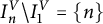
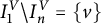

























Lemma 4.11 Let V and W be as in Lemma 4.4, and suppose that if
 $n-2\in I_{n-2}^{V}$
, then
 $n-1\in I_{n-2}^{V}$
also. Then, for each k in the range
 $1<k<n-2$
,
 $I_k^{W}$
contributes the same plusses as
 $I_{k}^{V}$
, except that if
 $I_{k}^{V}$
contributed a plus in the
 $n-3$
column of the Le diagram of V, then this plus is shifted one square left in the Le diagram of W.
Proof Recall that
 $I_1^W = I_1^V\cup \{n-3\}$
and that
 $n-2$
,
 $n-1$
, and n are not in
 $I_1^W$
.
If
 $n-3\not \in I_{k}^{V}$
, then by Lemma 4.4, we have
 $I_{k}^{W} = I_k^{V}\cup \{n-3\}$
. Because
 $n-3$
is the largest element of
 $I_1^{W}$
, this transformation leaves the disjoint paths unchanged, and so the plusses carry over from V to W directly.
If
 $n-3\in I_{k}^{V}$
, then
 $I_k^V$
must contribute a plus in column
 $n-3$
of the Le diagram of V, and by Lemma 4.4, we have
 $I_{k}^{W} = I_k^{V}\cup \{n-2\}$
. If
 $n-2$
supports no propagators in V, then certainly, no plusses appear in column
 $n-2$
of the Le diagram of V. If
 ${n-2}$
supports at least one propagator in V, then
 $n-2 \in I_{n-2}^V$
and so by hypothesis
 $n-1 \in I_{n-2}^V$
as well. By Lemma 4.10 item 3, the only necklace element of V containing
 $n-2$
is
 $I_{n-2}^{V}$
, and further with item 4, the plusses in column
 $n-2$
from
 $I_{n-2}^V$
and
 $I_{n-2}^W$
are different.
Because
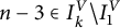 $n-3 \in I_k^V \setminus I_1^V$
, we must have a path in the Le diagram of V from some vertical edge i to the bottom edge
 $n-3$
. In the Le diagram of W, the index
 $n-3$
labels a vertical edge with no path from
 $I_k^W$
starting at it (because
 $n-3$
belongs to both
 $I_1^W$
and
 $I_k^W$
), and there must be a path leading to
 $n-2$
, because
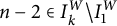 $n-2 \in I_k^W \setminus I_1^W$
. By the previous paragraph, no other path from
 $I_k^V$
could end at
 $n-2$
, and because the paths cannot cross, we conclude that the
 $i\rightarrow (n-3)$
path in the Le diagram of V must become an
 $i\rightarrow (n-2)$
path in the Le diagram of W. All other paths are unchanged.▪
We are now ready to prove the main result of this section, showing that the dimension of the positroid cell associated to each Wilson loop diagram is
 $3|\mathcal {P}|$
.
Theorem 4.12 Let
 $W = (\mathcal {P}, [n])$
be an admissible Wilson loop diagram. The number of plusses in the Le diagram of W is three times the number of propagators.
Proof The proof is by induction on the number of propagators.
First note that a Wilson loop diagram W with one propagator supported on vertices
 $$ \begin{align*}{i<i+1<j<j+1}\end{align*} $$
has a Le diagram consisting of a single row with
 $n-i$
boxes. The columns are labeled from left to right by
 $n, \ldots , i+1$
. By Algorithm 2.2, there are plusses in the
 $i+1$
, j, and
 $j+1$
positions.
Now, consider Wilson loop diagrams with
 $k>1$
propagators. By Lemma 4.1, it suffices to prove the result for weakly admissible Wilson loop diagrams with k propagators and no non-supporting vertices. By Lemma 4.2, it suffices to prove the result for at least one Wilson loop diagram from each dihedral orbit. In particular, we can restrict our attention to diagrams W which have a propagator p with the properties in Lemma 4.3.
Thus, W has one of the two configurations depicted in Figure 12, and by Remark 4.8, we can further assume that if
 $n-2 \in I_{n-2}^V$
, then
 $n-1 \in I_{n-1}^V$
as well. Let V be W with p removed.
From Lemma 4.6, we know how the shapes of the Le diagrams of V and W are related; let
 $\mathcal {A}$
and
 $\mathcal {B}$
be as described in that lemma and subsequent discussion.
Lemmas 4.7, 4.9, and 4.10 tell us that the three boxes of the bottom row of the Le diagram of W each have a plus, i.e., there are plusses in the positions
 $(n-3) \rightarrow (n-2)$
,
 $(n-3) \rightarrow (n-1)$
, and
 $(n-3) \rightarrow n$
. We will view these as the three “new” plusses required by the induction step and use Lemmas 4.7 through 4.11 to construct a pairing between the plusses of the Le diagram of V and the plusses of the Le diagram of W that are not in the bottom row. See Figure 14.
The Le diagrams for V and W in the setting of Theorem 4.12. The shaded regions indicate where the plusses match up perfectly from V to W, the bold (red) plusses exist if and only if
 $n-2 \in I_{n-2}^V$
, and the (blue) plusses in the bottom row of the Le diagrams of W diagrams are the three new plusses coming from the induction step.

The pairing is defined as follows:
-
• The plusses in the
$\mathcal {B}$
region of both Le diagrams are identical, so each plus in this region is paired with itself. -
• Every square containing a plus in the leftmost two columns (columns n and
$(n-1)$
) of
$\mathcal {A}$
for V also contains a plus in W, so these plusses are also paired with themselves. -
• The plusses in column
$n-3$
for V are paired with the corresponding plusses in column
$n-2$
for W. -
• If there is a plus in column
$n-2$
of
$\mathcal {A}$
in V, then Lemma 4.10 applies, so there is exactly one such plus in this column. If
$n-4 \not \in I_1^V$
, then pair this plus with the
$({n-5})\rightarrow (n-1)$
plus in W, whereas if
$n-4 \in I_1^V$
, then pair it with the
$({n-5}) \rightarrow n$
plus in W.





The first two points follow from Lemmas 4.7 through 4.10. The third point follows from Lemma 4.11, which tells us that column
 $n-3$
of V is identical to column
 $n-2$
of W (excluding the last row).
Finally, if
 $n-2 \not \in I_{n-2}^V$
, by Lemma 4.9, there are no plusses in column
 $n-2$
of the diagram of V, and all plusses have been accounted for. On the other hand, if
 $n-2 \in I_{n-2}^V$
, then we are in the setting of Lemma 4.10, and there is exactly one plus in column
 $n-2$
of the diagram of V. This plus is paired with the one plus in W yet unaccounted for, namely the one in position
 $(n-5) \rightarrow n$
or
 $(n-5) \rightarrow (n-1)$
, as described in points 4 and 6 of that lemma.
Therefore, the Le diagram of W contains
 $3(k-1)$
plusses in bijection with the plusses from the Le diagram of V and 3 new plusses in the bottom row, yielding
 $3k$
in total. Applying induction completes the proof.▪
5 Poles of Wilson loop integrals
Recall from Section 2.1 that each Wilson loop diagram defines a functional
 $I(W)$
, which associates a volume to the positroid cell
 $\Sigma (W)$
. In this section, we investigate the poles of the integrand of
 $I(W)$
.
Because SYM
 $N=4$
is a finite theory [Reference Alday and Maldacena9, Reference Positroids28], the scattering amplitudes (and thus the holomorphic Wilson loops
 $\,\mathfrak {W}_{k,n}$
) are finite. That is, for a fixed set of external particles
 $\mathcal {Z}$
, we must have
 $$ \begin{align*} \sum_{W \text{ s.t. } |\mathcal{P}| = k} I(W)(\mathcal{Z}) <\infty \;.\end{align*} $$
This holds if all poles of the integrands cancel. As a step toward this, in this section, we prove some results about the structure of the denominator
 $R(W)$
of the integrand, as defined in Definition 2.5.
The results of Section 3 allow us to relate the configuration of propagators in a Wilson loop diagram W to minors of
 $C(W)$
that contribute to
 $R(W)$
. The main result of this section is Theorem 5.4, which expresses the denominator
 $R(W)$
in terms of the Grassmann necklace of W. This simplifies the computation of
 $R(W)$
and allows us to directly relate the poles of the integrand to the combinatorics of the diagram.
For the duration of this section, fix an arbitrary ordering on the propagators of W. This imposes an ordering on the rows of
 $C(W)$
.
We first give an algorithm which extracts the required minors of
 $C(W)$
from the Grassmann necklace.
Algorithm 5.1 Let W = (P, [n]) be a Wilson loop diagram and C(W) be its associated matrix.
-
• For each i ∈ [n], we construct a factor r i as follows:
-
– Let
$S_i = \{p \in \mathcal{P} \ | \ I_{i-1}(p) \neq I_i(p)\}$
. (By convention, set I
0 = I
n
.) -
– Let r i be the determinant of the |S i |×|S i | minor of C(W) with rows indexed by S i and columns indexed by I i (S i ). If S i = ∅, set r i = 1.
-
-
• Define
$R = \prod_{i=1}^n r_i$
.


Each
 $r_i$
is the determinant of a minor determined by certain propagators of W. In particular, if a propagator p contributes one value to the ith element of the Grassmann necklace and a different value to the
 $(i-1)$
th element, then p is one of the propagators contributing to the minor. Specifically, the row associated to p and the column associated to the value that p contributes to the ith Grassmann Necklace element appear in the minor. Because each
 $r_i$
is simply the determinant of a particular submatrix of
 $C(W)$
and an ordering on the propagators has been fixed, the sign of each
 $r_i$
is well defined.
We also introduce the notation
 $\Delta _{I_i}$
to represent the determinant of the
 $k\times k$
minor of
 $C(W)$
with columns indexed by
 $I_i$
. Note that one summand of this determinant is given by
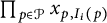 $\prod _{p \in \mathcal {P}}x_{p, I_i(p)}$
; the other summands are (up to sign) given by other bijections between the propagator set
 $\mathcal {P}$
and the vertex set
 $I_i$
.
Below, we show that the polynomial R associated to W by Algorithm 5.1 is equal to the denominator
 $R(W)$
from Definition 2.5, and that the ideal generated by R is the radical of the ideal generated by the product
 $\prod _{i=1}^n \Delta _{I_i}$
. First, however, we give a worked example of Algorithm 5.1.
Example 5.2 Consider the Wilson loop diagram in Figure 15. Assigning propagators p, q, r to rows
 $1,2,3$
, respectively, we obtain the matrix
 $$ \begin{align*} C(W) = \begin{bmatrix} a & b & 0 & 0 & 0 & c & d \\ e & f & 0 & 0 & g & h & 0 \\ i & j & 0 & k & l & 0 & 0 \end{bmatrix}. \end{align*} $$
The Grassmann necklace of this diagram is
 $$ \begin{align*}\Big(I_1 = \{1,2,4\},\ I_2 = \{2,4,5\},\ I_3 = \{4,5,6\},\ I_4=\{4,5,6\},\\ I_5=\{5,6,7\},\ I_6 = \{6,7,1\},\ I_7=\{7,1,2\}\Big). \end{align*} $$
Figure 15 indicates which vertex is contributed to
 $I_i$
by each propagator, for each
 $i \in [1,7]$
.
Example Wilson loop diagram for illustrating Algorithm 5.1 and bijections between propagators and vertices for each Grassmann necklace element.

From
 $I_1$
to
 $I_2$
, the propagators p and q change which vertices they contribute to; specifically, we have
 $I_1(p) = 1$
and
 $I_1(q)= 2$
, while
 $I_2(p) = 2$
and
 $I_2(q)= 5$
. On the other hand, r contributes 4 to both
 $I_1$
and
 $I_2$
. We therefore have
 $S_2 = \{p,q\}$
. The associated minors
 $\Delta _{I_2}$
and
 $r_2$
are therefore
 $$ \begin{align*} \Delta_{I_2}=\det\begin{bmatrix} b & 0 & 0 \\ f & 0 & g \\ j & k & l \end{bmatrix} = kgb, \qquad r_2 = \det\begin{bmatrix} b & 0 \\ f & g \end{bmatrix} = gb. \end{align*} $$
Continuing likewise, we get
 $r_3 = c$
,
 $r_4=1$
(because
 $I_4 = I_3$
),
 $r_5 = lhd$
, and
 $r_6 = i$
.
At
 $I_7$
, we see for the first time an irreducible quadratic factor. We have
 $S_7 = \{q,s\}$
with
 ${I_7(S_7) = \{ 1,2\}}$
,
 $\Delta _{I_7} = d(ej-fi)$
, and
 $r_7 = ej-fi$
.
The irreducible quadratic factor corresponds to the fact that q and s share an edge and contribute both endpoints of that edge to
 $I_7$
; see Proposition 5.3 below.
Finally, we have
 $r_1 = (af-be)k$
. Putting the previous calculations together, we obtain
 $$ \begin{align*} R = (af-be)kgbclhdi(ej-fi) \;, \end{align*} $$
which is square-free and contains all factors of
 $\prod _{i=1}^{n}\Delta _{I_i}$
. If one were to construct the denominator
 $R(W)$
associated to this Wilson loop diagram as per Definition 2.5, we would find that we have
 $R(W) = R$
.
We are now ready to begin proving the main result of this section. We begin with a proposition stating several facts about
 $\Delta _{I_i}$
and their relationship to
 $r_i$
.
Proposition 5.3 With notation as in Algorithm 5.1, the following statements hold.
-
(1) Each
$\Delta _{I_i}$
is homogeneous, as is each
$r_i$
. -
(2) Each
$\Delta _{I_i}$
splits into linear and quadratic factors. All linear factors of
$\Delta _{I_i}$
are single variables, and all irreducible quadratic factors are
$2\times 2$
determinants of single variables. -
(3) Quadratic factors in
$\Delta _{I_i}$
arise precisely when propagators p and q are supported on a common edge a with
$I_i(p)=a$
and
$I_i(q)=a+1$
. -
(4) The factor
$r_i$
divides
$\Delta _{I_i}$
. -
(5) The ideal generated by R is the radical of the ideal generated by
$\prod _{i=1}^{n}\Delta _{I_i}$
.


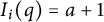


Proof
-
(1) The nonzero entries of
$C(W)$
are independent indeterminates, and so every
$i\times i$
minor of
$C(W)$
is either
$0$
or homogeneous of degree i. Thus, each
$\Delta _{I_i}$
and each
$r_i$
are homogeneous. -
(2) Viewing the determinant as a sum over permutations, and combining this with Corollary 2.4, we see that
$\Delta _{I_i}$
is a sum over bijections between
$I_i$
and
$\mathcal {P}$
. The nonzero terms in this sum are precisely those bijections such that each propagator is associated to one of its supporting vertices in
$I_i$
, because only those locations in
$C(W)$
are nonzero. Because the nonzero entries of
$C(W)$
are independent, there can be no cancellation between terms in this expansion.Suppose
$\Delta _{I_i}$
has an irreducible factor f. Let
$\mathcal {P}'$
be the set of propagators which contribute a variable to f, and let J be the set of vertices which contribute a variable to f.The first claim is that the minor of
$C(W)$
associated to
$\mathcal {P}'$
and J is precisely f.Proof of claim: By the structure of determinants, we know that
$\Delta _{I_i} = fg$
, where g involves only variables associated to propagators not in
$\mathcal {P}'$
and associated to vertices not in J.Expanding out
$fg$
yields a signed sum of monomials. Because there is no cancellation between terms, this means that the full expansion over permutations of
$\Delta _{I_i}$
contains no other nonzero terms and hence no other variables. Therefore,
$\Delta _{I_i}$
is equal to the determinant of the matrix obtained by taking the submatrix of
$C(W)$
with columns indexed by
$I_i$
and setting any variables not appearing in
$\Delta _{I_i}$
to
$0$
. This new matrix is, up to permutations of rows and columns, a block matrix with one block for
$\mathcal {P}'$
and J and the other block for the complements. Thus, its determinant, and hence also
$\Delta _{I_i}$
, is the product of the minors for these two blocks. By considering which variables appear, these two factors must also be f and g, and so, in particular, f is the minor of
$C(W)$
associated to
$\mathcal {P}'$
and J. This proves the claim.A consequence of this claim is that every linear factor of
$\Delta _{I_i}$
is a
$1\times 1$
minor of
$C(W)$
, hence is a single variable, and every irreducible quadratic factor of
$\Delta _{I_i}$
is a
$2\times 2$
minor of
$C(W)$
, hence is a
$2\times 2$
determinant of single variables.All that remains is to prove that
$\Delta _{I_i}$
has no irreducible factors of degree 3 or more. Suppose, by way of contradiction, that f is a factor of
$\Delta _{I_i}$
of degree
$\geq 3$
. Without loss of generality,Footnote
4
we may assume
$i\in I_i$
and that i contributes to f. Finally, we can suppose that W is minimal with respect to the number of propagators among diagrams with an irreducible factor of degree
$\geq $
3.Let p be the propagator such that
$I_i(p) = i$
. There are two cases to consider: when p is supported on the edge
$i-1$
or the edge i. These are illustrated in Figure 16.Figure 16:The two cases in the proof that no factors of
$\Delta _{I_i}$
have degree 3 or more.Case 1: Suppose
$p = (i-1, m)$
. Then, p has one end on the
$(i-1)$
th edge, and
$I_{i+1}(p) = m$
by Remark 3.13.Let
$T = \mathcal {P}_{in}(p)$
be the set of propagators inside p in the
$<_i$
order. By Remark 3.9,
$I_i$
and
$I_{i+1}$
can only differ once p contributes to
$I_{i+1}$
, so
$I_i(q) = I_{i+1}(q)$
for each
$q \in T \backslash \{p\}$
. Thus, every propagator inside p contributes before m, and if a propagator contributes m in
$I_i$
, then it must lie outside p.If neither m nor
$m+1$
appears in
$I_i$
, then by Corollary 3.16, we have
$V(p) \cap I_i = \{i\}$
, and so the row of p in the matrix of
$\Delta _{I_i}$
has only one nonzero entry; hence
$\Delta _{I_i}$
has a linear factor contributed by p and i, which is a contradiction to the fact that i contributes to f. So we must have at least one of m and
$m+1$
in
$I_i$
. However, all propagators in T contribute to
$I_{i}$
strictly before m by the previous paragraph so, after permuting rows and columns as needed, the matrix giving
$\Delta _{I_i}$
has the form where A is the
$$ \begin{align*} \begin{bmatrix} A & B \\ 0 & C\end{bmatrix} \;, \end{align*} $$
$|T|\times |T|$
matrix indexed by the propagators in T and the vertices in
$I_i(T)$
. No other propagators can be supported on these vertices, because all other propagators are outside p, and p is the first propagator supported at i; this explains the zero block. Therefore,
$\Delta _{I_i} = \pm \det A \det C$
, and both factors are nontrivial, because at least one of m and
$m+1$
appears in
$I_i$
.
Because
$p\in \mathcal {P}_{in}(p)$
, we have
$f|\det A$
, and if we remove a propagator outside p that contributes either m or
$m+1$
, we get a diagram
$W'$
with fewer propagators for which
$\det A | \Delta _{I^{W'}_i}$
still holds, hence
$f|\Delta _{I^{W'}_i}$
. This contradicts the minimality of our choices.Case 2: Suppose
$p = (i, m)$
, i.e., p has an end on the ith edge. If no other propagators are supported on the vertex i, then the corresponding column of
$C(W)$
has only one nonzero entry in it, and so
$\Delta _{I_i}$
has a linear factor contributed by p and i; as above, this is a contradiction. Because p is the first propagator in the ordering imposed by
$I_i$
, it is the clockwise-most propagator supported on i (by Remark 3.8). Because there are multiple propagators supported on i, there must be a q ending on edge i, such that
$I_i(q) = i+1$
, that is, second clockwise-most propagators supported by i (see Figure 16). Write
$q = (i, j)$
for the support of q. The situation for q is very similar to Case 1: in particular, we have
$I_{i+1}(q) = j$
by Lemma 3.12, and so if
$j\in I_i$
, then the propagator which contributes j is outside q.Similarly to Case 1, let
$T = \mathcal {P}_{in}(q) \cup \{p\}$
in the
$<_i$
order. All propagators in T contribute to
$I_i$
strictly before j, and no other propagators are supported on vertices strictly before j. Thus, after permuting rows and columns as needed, the matrix giving
$\Delta _{I_i}$
has the form where A is the submatrix indexed by the propagators in T and the vertices in
$$ \begin{align*} \begin{bmatrix} A & B \\ 0 & C\end{bmatrix} \;, \end{align*} $$
$I_i(T)$
. Again, there are two cases to consider. If some vertex j or larger (with respect to
$<_i$
) belongs to
$I_i$
, then B and C are at least one column wide, and so the block form of the matrix gives a nontrivial factorization of
$\Delta _{I_i}=\pm \det A\det C$
. This yields a contradiction as in Case 1:
$f|\det A$
and removing a propagator not in T gives a smaller diagram with a factor of degree
$\geq $
3, which contradicts our minimality assumption.
On the other hand, if no vertex
$\geq _i j$
is in
$I_i$
, then we have
$\Delta _{I_i} = \det A$
. Looking in more detail into A, note that the only vertices that support both p and q and also belong to
$I_i$
are i and
$i+1$
. Hence,
$$ \begin{align*} A = \begin{bmatrix} D & 0 \\ E & F\end{bmatrix}\; , \end{align*} $$
where D is the
$2\times 2$
matrix indexed by the propagators p and q and the vertices i and
$i+1$
. Thus, p and i contribute to a quadratic factor of
$\Delta _{I_i}$
, once again contradicting our assumptions.All cases have now been covered, and so
$\Delta _{I_i}$
has only irreducible factors of degree
$2$
or less. -
(3) Suppose propagators p and q are supported on a common edge a, with
$I_i(p)=a$
and
${I_i(q)=a+1}$
. Let
$x_{p,a},x_{p,a+1},x_{q,a},x_{q,a+1}$
be the associated variables in
$C(W)$
. For any fixed bijection
$\sigma $
from
$\mathcal {P}\setminus \{p,q\}$
to
$I_i \setminus \{a,a+1\}$
for which each propagator is supported on its image under the bijection, we can extend
$\sigma $
to a bijection from propagators to
$I_i$
in two ways: either
$p\mapsto a$
and
$q\mapsto a+1$
or
$p\mapsto a+1$
and
$q\mapsto a$
. The sum of the contributions of all these bijections to
$\Delta _{I_i}$
is therefore the product of
$(x_{p,a}x_{q,a+1}-x_{p,a+1}x_{q,a})$
with the minor coming from
$\mathcal {P}\setminus \{p, q\}$
and
$I_i \setminus \{a,a+1\}$
. Because there is no cancellation of terms in the expansion of
$\Delta _{I_i}$
, if any other terms appear, then they will cause a factor which is not in the form described at the beginning of the proof of part (2). Therefore, no such terms exist, and
$(x_{p,a}x_{q,a+1}-x_{p,a+1}x_{q,a})$
is a factor of
$\Delta _{I_i}$
.Now, let f be a quadratic factor of
$\Delta _{I_i}$
. By part (2), we know that f is a
$2\times 2$
minor coming from two propagators, call them p and q, and two vertices, call them a and b, and assume that
$a <_i b$
. It remains to show that
$b = a+1$
. From this, we can conclude that p and q each have one end on edge a.As in the proof of part (2), make a new admissible diagram by removing the propagators which come before those contributing to f in the order imposed by
$I_i$
. Without loss of generality, we may assume
$i=a$
. The cases in the proof of part (2) show how
$\Delta _{I_i}$
factors. In particular, the vertices supporting the other end of p either do not appear in
$I_i$
, or they contribute to a different factor of
$\Delta _{I_i}$
than p and a do. By assumption, b contributes to the same factor as a. Therefore,
$(a,b)$
is an edge defining an end of p, that is,
$b = a+1$
. -
(4) If
$S_i = \emptyset $
, then
$r_i = 1$
, and we immediately have
$r_i | \Delta _{I_i}$
; otherwise, let
$p\in S_i$
.Note that
$\Delta _{I_i}$
is homogeneous linear in the variables of the row corresponding to p. By part (2), either exactly one variable in the row corresponding to p appears in
$\Delta _{I_i}$
and this variable is a factor of
$\Delta _{I_i}$
, or exactly two variables from the row corresponding to p appear in
$\Delta _{I_i}$
and they appear as part of a quadratic factor. In the first case, let the variable be x. Then, x is a factor of
$\Delta _{I_i}$
. Therefore, x must appear in the row of p and column of
$I_i(p)$
, i.e.,
$x = x_{p, I_i(p)}$
. Thus, x also appears in
$r_i$
. Because the matrix for
$r_i$
is a minor of the matrix for
$\Delta _{I_i}$
, and every term in
$\Delta _{I_i}$
involves x, we also have that every term in
$r_i$
involves x, so x is a factor of both
$r_i$
and
$\Delta _{I_i}$
and is the only variable from this row in either polynomial.Now, suppose two variables from the row p appear in a quadratic factor f of
$\Delta _{I_i}$
. By part (3), there is another propagator q and an edge a such that f is the
$2\times 2$
minor coming from
$p, q$
and
$a, a+1$
. There are two situations which can occur, either
$I_i(p)=a$
and
$I_i(q)=a+1$
, or
$I_i(q)=a$
and
$I_i(p)=a+1$
. We show that in both cases, it follows that
$q \in S_i$
as well.In both cases, because we have
$I_{i-1}(p)\neq I_{i}(p)$
by assumption, it follows from Lemma 3.12 that
${I_{i-1}(p) <_{i-1} I_{i}(p)}$
, and no other vertex supporting p lies between
$I_{i-1}(p)$
and
$I_{i}(p)$
. If
$I_i(q)=a$
, then q lies clockwise of p and q contributes before p in
$I_i$
. This means that
$I_{i-1}(p)=a$
and so
$I_{i-1}(q)\neq a$
. Thus,
$q\in S_i$
and so f is a factor of
$r_i$
.Now, consider the case where
$I_i(q) = a+1$
, and suppose for contradiction that
$q \not \in S_i$
, i.e., that
$I_{i-1}(q) = a+1$
. Because
$I_{i-1}(p) \neq a$
, there must be some other propagator s with
$I_{i-1}(s) = a$
(else q contributes a to
$I_{i-1}$
). This propagator cannot lie on edge a, because Remark 3.13 would imply that
$I_i(s) \in \{a, a+1\}$
, contradicting the fact that
$I_i(p) = a$
and
$I_i(q) = a+1$
; thus s has an end on edge
$(a-1)$
and is inside p in the
$<_k$
order where
$p=(k,a)$
.Say
$s = (j,a-1)$
with
$i-1 \leq _{i-1} k+1 \leq _{i-1} j+1$
. But by Lemma 3.10, if
$I_{i-1}(s) = a$
, then a cannot be maximal in the support of s with respect to
$<_{i-1}$
; thus, we must have
$i-1 = j+1$
, and we are in the situation in Figure 17.Figure 17:In order to obtain
$I_{i-1}(s) = a$
, propagators s and p must each have an end on edge
$(i-2)$
.Because p changed its association from
$I_{i-1}$
to
$I_i$
, we have
$I_{i-1}(p) = i-1$
by Lemma 3.12. From Figure 17 and Remark 3.9, p contributes first to
$I_{i-1}$
and proceeds identically to
$I_i$
for all vertices inside p in the
$<_{i-1}$
ordering, implying that
$I_{i-1}(s) = I_i(s)$
. Because
$I_{i-1}(s) = a$
and
$I_i(s) \neq a$
, this is a contradiction.Thus,
$q\in S_i$
after all, and so f is a factor of
$r_i$
as required. -
(5) If W has zero propagators, then all
$I_i=\emptyset $
and both R and
$\prod _{i=1}^n \Delta _{I_i}$
are equal to
$1$
, so the result holds in this case. Now, assume W has at least one propagator.First, we show that every factor of
$\prod _{i=1}^n \Delta _{I_i}$
divides R. Take an irreducible factor f of
$\prod _{i=1}^n \Delta _{I_i}$
. There exists some i such that
$f|\Delta _{I_i}$
but
$f\!\!\nmid \!\! \Delta _{I_{i-1}}$
, because otherwise the variables corresponding to the propagators contributing to f which do not themselves appear in f could never appear, contradicting Lemma 3.12. If f is a linear factor, say from associating propagator p to vertex a, then
$I_{i}(p)=a$
and
$I_{i-1}(p)\neq a$
, so this factor appears in
$r_i$
. If f is a quadratic factor, say from associating propagators p and q to vertices a and
$a+1$
, respectively, then again we cannot have both
$I_{i-1}(p) = a$
and
$I_{i-1}(q) = a+1$
, else f divides
$\Delta _{i-1}$
. However, by the proof of part (4), if one of
$p,q$
belongs to
$S_i$
, then the other does as well. Thus, f divides
$r_i$
.Next, we need to show that R is square-free. Suppose
$f^2|R$
. If f is a linear factor, say from associating propagator p to vertex a, then there must be two distinct points in the Grassmann necklace algorithm where p changes from not being associated to vertex a to being associated to vertex a. This contradicts Lemma 3.12. Now, suppose f is a quadratic factor, say from propagators p and q supported on edge a with p clockwise to q on the edge. In this case, it is not possible for any
$I_i$
to associate p to
$a+1$
and q to a. Furthermore, we know by part (4) that p changes from not being associated to a to being associated to a if and only if q changes from not being associated to
$a+1$
to being associated to
$a+1$
. Thus,
$f^2|R$
implies that in the Grassmann necklace, p must change twice from not being associated to vertex a to being associated to vertex a. This is again a contradiction, and so R is square-free.From the arguments above, we have that
$R|\prod _{i=1}^n \Delta _{I_i}$
(from part (4)), R contains all factors of
$\prod _{i=1}^n \Delta _{I_i}$
, and R is square-free. Therefore, the ideal generated by R is the radical of the ideal generated by
$\prod _{i=1}^n \Delta _{I_i}$
.














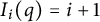








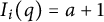



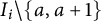




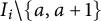




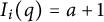

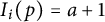





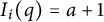






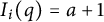


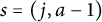












We are now ready to prove the main theorem of this section. We use the facts about
 $\Delta _{I_i}$
and R above to show that the denominator
 $R(W)$
of the integrand of
 $I(W)$
is given by Algorithm 5.1.
Theorem 5.4 Given any admissible Wilson loop diagram W, let
 $(I_1, \ldots I_n)$
be the associated Grassmann necklace. Then,
 $R(W)$
as defined in Definition 2.5 is equal to the R constructed by Algorithm 5.1. Furthermore, the ideal generated by
 $R(W)$
is the radical of the ideal generated by
 $\prod _{i=1}^n \Delta _{I_i}$
, where
 $\Delta _{I_i}$
is the determinant of the
 $k \times k$
minor indicated by
 $I_i$
.
Proof The equivalence of the ideal generated by R and the radical of the ideal generated by
 $\prod _{i=1}^n \Delta _{I_i}$
are due to Proposition 5.3. It remains to prove that
 $R(W)$
is the R of Algorithm 5.1.
To this end, first note that
 $R(W)$
and R both have total degree
 $4|\mathcal {P}|$
; the degree of
 $R(W)$
is immediate from the definition while that of R follows from Remark 3.13. By Proposition 5.3, every factor of R is either a quadratic factor coming from two propagators supported on a common edge or a single variable coming from a support vertex of a propagator not appearing in a quadratic factor. The factors of each
 $R_e$
making up
 $R(W)$
in the notation of Definition 2.5 are all of this form, and every such factor occurs. Hence, every factor of R divides
 $R(W)$
. Finally, because R is square-free, this implies that
 $R(W)$
is a scalar multiple of R.
Finally, we need to check the scalar. By Definition 2.5, each linear factor appears with coefficient
 $1$
, and each
 $2\times 2$
determinant factor appears with the same sign as the determinant of the corresponding minor in
 $C(W)$
. Therefore,
 $R=R(W)$
.
Thus, we have shown a deep relationship between the physically derived poles of the integrand
 $\Omega (W)$
and the geometry and combinatorics associated to the diagrams W. This is yet another piece of substantial evidence indicating that the positroid representation of Wilson loop diagrams is the correct geometric object to use when considering the Wilson loop amplitudes geometrically.