1. Introduction
The mathematical formulation for the self-induced motion of a thin vortex filament was given by Da Rios (Reference Da Rios1906) and rediscovered by others later (Arms & Hama Reference Arms and Hama1965; Ricca Reference Ricca1991). The dynamics of such a classical (Widnall Reference Widnall1972) or low-temperature quantum (Boffetta et al. Reference Boffetta, Celani, Dezzani, Laurie and Nazarenko2009) vortex filament are governed by the Biot–Savart law
 $$\begin{eqnarray}\boldsymbol{r}_{t}=\frac{{\it\kappa}}{4{\rm\pi}}\int _{\ell }\frac{(\boldsymbol{s}-\boldsymbol{r})\times \text{d}\boldsymbol{s}}{|\boldsymbol{s}-\boldsymbol{r}|^{3}},\end{eqnarray}$$
where curve
 $\boldsymbol{r}$
represents the spatial curve modelling the vortex filament at any time
 $t$
,
 $\boldsymbol{s}$
represents the variable of integration,
 ${\it\kappa}$
denotes the strength of the filament (circulation), and
 $\ell$
is the path along which the filament lies. This representation is non-local, meaning that distant parts of the filament can affect the behaviour of the filament at a specific point. Since this equation is non-local, it is difficult to solve for most vortex configurations. Still, a number of approximations of both analytical and numerical flavours have been discovered. The difficulty and usefulness of such approximation methods will depend strongly on the type of filament solution sought. Due to the mathematical and computational difficulties in studying (1.1), the local induction approximation (LIA) is sometimes used to replace the integral in (1.1) with a far simpler relation, namely
 $$\begin{eqnarray}\boldsymbol{r}_{t}=\frac{{\it\kappa}}{4{\rm\pi}}\ln (1/{\it\epsilon})\boldsymbol{t}\times \boldsymbol{n},\end{eqnarray}$$
where
 $\boldsymbol{t}$
is the tangent vector,
 $\boldsymbol{n}$
is the normal vector to
 $\boldsymbol{r}$
scaled with the scalar curvature. Here
 ${\it\epsilon}$
is a small distance parameter signifying that we have removed the logarithmic singularity and are approximating the region near this singularity. The right-hand side of (1.2) is the binormal vector (up to scaling). While (1.2) defines a nonlinear vector partial differential equation, its solution is still simpler than that of the non-local and singular equation (1.1). The LIA is useful when the vortex filaments are very thin, which is true for instance in the case of quantized vortex filaments in superfluid helium. For classical vortex filaments, the LIA has well-known limitations. Therefore, it is certainly desirable to be able to study solutions of (1.1) in the context of classical vortex filaments.
In the present paper, we shall be interested in a Cartesian representation of a thin helical vortex filament (since from the Cartesian representation the shape and motion of the filament will be easiest to visualize), so let us write
 $\boldsymbol{r}=(X,Y,Z)$
. Equation (1.1) gives the vector relation
 $$\begin{eqnarray}(X_{t},Y_{t},Z_{t})=\frac{{\it\kappa}}{4{\rm\pi}}\int \frac{(s_{1}-X,s_{2}-Y,s_{3}-Z)\times (\text{d}s_{1},\text{d}s_{2},\text{d}s_{3})}{\left[(s_{1}-X)^{2}+(s_{2}-Y)^{2}+(s_{3}-Z)^{2}\right]^{3/2}}.\end{eqnarray}$$
This gives the time evolution for each component of
 $\boldsymbol{r}$
. If we desire a solution curve
 $\boldsymbol{r}$
to the Biot–Savart law (1.1), we must be able to solve (1.3) for the position components. Depending on the type of solution sought, solving this system may vary from difficult to impossible.
To overcome the singularity inherent in (1.3), we shall apply the LIA near the singular point, while we keep the full Biot–Savart law outside of such a region. In other words, the time evolution of the solution curve
 $\boldsymbol{r}=(X,Y,Z)$
shall consist of one part giving a local effect very near each point on the curve (the LIA term) and one part giving the non-local effects (sufficiently removed from the point). This approximation should take the form of
 $$\begin{eqnarray}\boldsymbol{r}_{t}=-\frac{{\it\kappa}}{4{\rm\pi}}\ln ({\it\epsilon})\boldsymbol{t}\times \boldsymbol{n}+\frac{{\it\kappa}}{4{\rm\pi}}\int _{|\boldsymbol{s}-\boldsymbol{r}|>{\it\epsilon}}\frac{(s_{1}-X,s_{2}-Y,s_{3}-Z)\times (\text{d}s_{1},\text{d}s_{2},\text{d}s_{3})}{\left[(s_{1}-X)^{2}+(s_{2}-Y)^{2}+(s_{3}-Z)^{2}\right]^{3/2}}.\end{eqnarray}$$
This approximation method has been suggested and used in numerical studies of superfluid vortex filament dynamics (Schwarz Reference Schwarz1985), and the appeal of this method is that it permits one to directly compare the LIA solutions with the Biot–Savart solutions. In this way, one can determine the influence of non-locality on a vortex filament. This approach gives useful analytical information about the time evolution of helical vortex filaments under the Biot–Savart dynamics.
Regarding helical filaments, the ‘cut-off’ method based on the oscillating vortex ring has been employed to study helical vortex filaments (Widnall Reference Widnall1972). This method also approximates the inner region of the vortex cross-section. Under appropriate assumptions, the method reduces to the LIA. An analysis of the approach was conducted by Moore & Saffman (see Moore & Saffman Reference Moore and Saffman1972 and Saffman Reference Saffman1992). Using the cut-off method Ricca (Reference Ricca1994) obtained analytical results in the small-helix-diameter and large-torsion limit, and demonstrated that torsion strongly influences the motion of helical filaments. Results have been given in the small-pitch (large wavenumbers) and small-amplitude regime (Widnall Reference Widnall1972; Ricca Reference Ricca1994), while Ricca (Reference Ricca1994) also gives an analytic result for the infinite-torsion case, valid when the pitch is small (wavenumber is large). Additional studies on the cut-off method (Boersma & Wood Reference Boersma and Wood1999) have improved on the aforementioned analytical results. In addition to results for the Biot–Savart law, note that analytical results are common under the LIA (Zhou Reference Zhou1997), which is much simpler to solve in the helical case (Kida Reference Kida1981; Sonin Reference Sonin2012).
In the present paper, we study helical vortex filaments under Biot–Savart dynamics in the Cartesian frame. Doing so, we quickly recover the representations for the rotational and transverse velocity of the helical filament in terms of the wavenumber and radius of the helix. The benefit of considering the results in Cartesian form is that we immediately can visualize the structure of the filament, so we can use these velocities to give a closed-form position of the helical filament curve at an arbitrary time
 $t>0$
. As opposed to using the cut-off approximation in the way mentioned above, we simply replace the ‘inner’ dynamics in the Biot–Savart law directly with the LIA by using (1.4), while the non-local effects remain in integral form. Furthermore, by using the LIA for the local region, we can meaningfully compare the non-local formulation with existing results valid strictly under the LIA. In our study of helical filaments, we do not assume that the radius of the helical filament,
 $A$
, tends to zero. Therefore, torsion
 ${\it\tau}$
must be bounded like
 $0<{\it\tau}<2A^{-1}$
where
 $A$
is the amplitude of the helix. In § 2, we obtain the exact form of the transverse and rotational velocity for a helical filament in terms of both the local (LIA) contribution and an outer contribution due to the Biot–Savart dynamics. The latter contribution for each is given as a finite integral. In § 3, we give analytical approximations to these integrals, which in turn gives us approximations to the transverse and rotational velocities. Comments on results obtained via the cut-off method are made along the way. In § 4, we compare the exact solutions obtained in § 2 with both the LIA and the approximations of § 3. In § 5, we show that the ratio of translational and rotational velocity equals
 $A^{2}k$
in the large-
 $k$
limit. This means that the helical vortex reduces to a cylindrical vortex sheet in the
 $k\rightarrow \infty$
limit (i.e. in the limit where pitch becomes small), which is what we expect of any solution (the LIA trivially satisfies this requirement). Qualitative features of the solutions are discussed in § 6.
2. Time evolution of a helical filament
The helical filament corresponds to one possible parameterization of
 $\boldsymbol{r}$
. For simplicity, we align the filament along one axis (here we shall choose the
 $x$
-axis), so in Cartesian coordinates, we write
 $$\begin{eqnarray}\boldsymbol{r}(x,t)=(x+{\it\beta}t,A\cos (kx-{\it\omega}t+x_{0}),A\sin (kx-{\it\omega}t+x_{0})).\end{eqnarray}$$
The motion of this filament is governed by
 ${\it\beta}$
(which is the transverse velocity of a helical wave along the line filament corresponding to
 $A=0$
) and
 ${\it\omega}$
(which is the rotational velocity). Therefore, if we can determine
 ${\it\beta}$
and
 ${\it\omega}$
, we will know the position of the helical filament (2.1) for any value of time. For simplicity, we shall scale time by
 ${\it\kappa}/8{\rm\pi}$
to remove the corresponding factor of the integral (1.4). In this parameterization about the
 $x$
-axis, we should have
 $\boldsymbol{t}\times \boldsymbol{n}=|\boldsymbol{r}_{s}|^{-3}\boldsymbol{r}_{s}\times \boldsymbol{r}_{ss}$
for the helix (where
 $s$
denotes arclength,
 $x$
will be a parameterization of arclength).
Notice that, under the assumption of a helical filament (2.1), relevant quantities in (1.4) can be parameterized like
 $s_{1}=S$
,
 $s_{2}=A\cos (kS-{\it\omega}t+x_{0})$
, and
 $s_{3}=A\sin (kS-{\it\omega}t+x_{0})$
. We obtain from (1.4) the system
 $$\begin{eqnarray}\displaystyle {\it\beta}=-\frac{2\ln ({\it\epsilon})A^{2}k^{3}}{(1+A^{2}k^{2})^{3/2}}+2A^{2}k\int _{|S-x|>{\it\epsilon}}\frac{1-\cos (k[S-x])}{[(S-x)^{2}+2A^{2}(1-\cos (k[S-x]))]^{3/2}}\text{d}S, & & \displaystyle\end{eqnarray}$$
 $$\begin{eqnarray}\displaystyle & & \displaystyle A{\it\omega}\sin (kx-{\it\omega}t+x_{0})=-\frac{2\ln ({\it\epsilon})Ak^{2}}{(1+A^{2}k^{2})^{3/2}}\sin (kx-{\it\omega}t+x_{0})\nonumber\\ \displaystyle & & \displaystyle \quad +\,2A\!\int _{|S-x|>{\it\epsilon}}\frac{\sin (kS-{\it\omega}t+x_{0})-\sin (kx-{\it\omega}t+x_{0})-k(S-x)\cos (kS-{\it\omega}t+x_{0})}{[(S-x)^{2}+2A^{2}(1-\cos (k[S-x]))]^{3/2}}\text{d}S,\nonumber\\ \displaystyle & & \displaystyle\end{eqnarray}$$
 $$\begin{eqnarray}\displaystyle & & \displaystyle -A{\it\omega}\cos (kx-{\it\omega}t+x_{0})=\frac{2\ln ({\it\epsilon})Ak^{2}}{(1+A^{2}k^{2})^{3/2}}\cos (kx-{\it\omega}t+x_{0})\nonumber\\ \displaystyle & & \displaystyle \quad -\,2A\!\int _{|S-x|>{\it\epsilon}}\frac{\cos (kS-{\it\omega}t+x_{0})-\cos (kx-{\it\omega}t+x_{0})+k(s-x)\sin (kS-{\it\omega}t+x_{0})}{[(S-x)^{2}+2A^{2}(1-\cos (k[S-x]))]^{3/2}}\text{d}S.\nonumber\\ \displaystyle & & \displaystyle\end{eqnarray}$$
 ${\it\omega}$
which provides the rotational motion. In particular, we take i times equation (2.3) and subtract equation (2.4), from which we obtain
 $$\begin{eqnarray}\displaystyle {\it\omega}\,\text{e}^{\text{i}[kx-{\it\omega}t+x_{0}]}\! & = & \displaystyle \!-\frac{2\ln ({\it\epsilon})k^{2}}{(1+A^{2}k^{2})^{3/2}}\text{e}^{\text{i}[kx-{\it\omega}t+x_{0}]}\nonumber\\ \displaystyle & & \displaystyle +\,2\text{e}^{\text{i}[kx-{\it\omega}t+x_{0}]}\!\int _{|S-x|>{\it\epsilon}}\frac{(1-\text{i}k[S-x])\text{e}^{\text{i}k[S-x]}-1}{[(s-x)^{2}+2A^{2}(1-\cos (k[S-x]))]^{3/2}}\text{d}S.\qquad\end{eqnarray}$$
Simplifying this equation, and noting that the integral should have both a real and imaginary part, we obtain (putting
 ${\it\sigma}=S-x$
)
 $$\begin{eqnarray}\displaystyle {\it\omega} & = & \displaystyle -\frac{2\ln ({\it\epsilon})k^{2}}{(1+A^{2}k^{2})^{3/2}}+2\int _{|{\it\sigma}|>{\it\epsilon}}\frac{\cos (k{\it\sigma})-1+k{\it\sigma}\sin (k{\it\sigma})}{[{\it\sigma}^{2}+2A^{2}(1-\cos (k{\it\sigma}))]^{3/2}}\text{d}{\it\sigma}\nonumber\\ \displaystyle & & \displaystyle +\,2\text{i}\int _{|{\it\sigma}|>{\it\epsilon}}\frac{\sin (k{\it\sigma})-k{\it\sigma}\cos (k{\it\sigma})}{[{\it\sigma}^{2}+2A^{2}(1-\cos (k{\it\sigma}))]^{3/2}}\text{d}{\it\sigma}.\end{eqnarray}$$
Note that the integrand of the integral multiplying the i is an odd function, therefore the integral over
 $(-\infty ,{\it\epsilon})$
is the negative of the integral over
 $({\it\epsilon},\infty )$
, hence this integral is zero. This makes sense, as
 ${\it\omega}$
should be real-valued. On the other hand, the real part of the integral has an integrand which is an even function, so the total integral is just twice the integral over
 $({\it\epsilon},\infty )$
. We therefore obtain
 $$\begin{eqnarray}\displaystyle {\it\omega}=-\frac{2\ln ({\it\epsilon})k^{2}}{(1+A^{2}k^{2})^{3/2}}+4\int _{{\it\epsilon}}^{\infty }\frac{\cos (k{\it\sigma})-1+k{\it\sigma}\sin (k{\it\sigma})}{[{\it\sigma}^{2}+2A^{2}(1-\cos (k{\it\sigma}))]^{3/2}}\text{d}{\it\sigma}. & & \displaystyle\end{eqnarray}$$
In a similar manner, the translational velocity along the
 $x$
-axis is given by
 $$\begin{eqnarray}\displaystyle {\it\beta}=-\frac{2\ln ({\it\epsilon})A^{2}k^{3}}{(1+A^{2}k^{2})^{3/2}}+4A^{2}k\int _{{\it\epsilon}}^{\infty }\frac{1-\cos (k{\it\sigma})}{[{\it\sigma}^{2}+2A^{2}(1-\cos (k{\it\sigma}))]^{3/2}}\text{d}{\it\sigma}. & & \displaystyle\end{eqnarray}$$
With
 ${\it\omega}$
and
 ${\it\beta}$
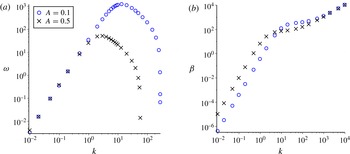
known, we can describe the motion of the helical vortex filament (2.1) exactly. In figure 1, we plot the rotational and translational velocity parameters for various values of the physical constants.
Numerical plots of (a) the rotational velocity,
 ${\it\omega}$
, and (b) transverse velocity,
 ${\it\beta}$
, of a helical vortex filament when non-local dynamics are accounted for. The results use the LIA near the logarithmic singularity, so these are the solutions (2.7) and (2.8), respectively. Note that we set
 ${\it\epsilon}=10^{-5}$
in all plots. The precise value of
 ${\it\epsilon}$
is not important, since a change in it results in a scaling of the plots, therefore the value of
 ${\it\epsilon}$
does not influence the qualitative features of the solutions.

The integral term in (2.7) is equivalent to equation (19) of Widnall (Reference Widnall1972), except that integral was approximated in a different way by using the cut-off approximation. In that method, a function of the same singular order is added and subtracted under the integral, in order to remove the logarithmic divergence. The remaining singularity is shifted to an auxiliary integral, which can itself be evaluated in terms of a cosine integral. The quantities were Fourier transformed in Widnall (Reference Widnall1972), which helps in computation of the integrals (see equation (36) of Widnall Reference Widnall1972). The resulting approximations were then solved numerically. While the approach of Widnall and that given here are similar (in the sense that both offer approximations for the velocities of the helical vortex filament), the approach here is connected nicely with the LIA, and hence is more useful for direct comparison with the LIA, which in turn allows one to ascertain the direct influence of the non-locality more easily.
We see that there exists a particular finite value of the wavenumber
 $k$
for which the rotational velocity of the filament is maximal. On the other hand, the behaviour of the translational velocity is a bit more complicated. For small
 $k$
,
 ${\it\beta}$
scales like
 ${\it\beta}\sim k^{2}$
, while for large
 $k$
, the integral term dominates, giving
 ${\it\beta}\sim k$
.
As a final remark in this section, let us note that the representation (2.1) is formulated in the external observer’s frame of reference. Here,
 ${\it\beta}$
has the interpretation of being the translation of the helix, while
 ${\it\omega}$
is the observed rotational velocity or frequency parameter. An intrinsic representation (the frame moving with the filament) of the helical filament would take the form
 $$\begin{eqnarray}\displaystyle \boldsymbol{r}=(X(t),A\cos (kX(t)-{\it\phi}t+x_{0}),A\sin \cos (kX(t)-{\it\phi}t+x_{0})), & & \displaystyle\end{eqnarray}$$
where
 $X(t)=x+{\it\beta}t$
(as we have in (2.1)) and
 ${\it\phi}$
is the rotational velocity or frequency parameter observed in the reference frame moving with the helical filament. One does not need separate derivations in order to recover the solution (2.9), since this representation is necessarily equivalent to that in the external observer’s frame, (2.1). Clearly, we must have
 $kx-{\it\omega}t=kX(t)-{\it\phi}t=kx+k{\it\beta}t-{\it\phi}t$
, and therefore
 ${\it\phi}={\it\omega}+k{\it\beta}$
. For the Biot–Savart law with regularization (1.4), we obtain the dispersion relation
 $$\begin{eqnarray}\displaystyle {\it\phi}=-\frac{2\ln ({\it\epsilon})k^{2}}{\sqrt{1+A^{2}k^{2}}}+4\int _{{\it\epsilon}}^{\infty }\frac{(A^{2}k^{2}-1)[1-\cos (k{\it\sigma})]+k{\it\sigma}\sin (k{\it\sigma})}{[{\it\sigma}^{2}+2A^{2}(1-\cos (k{\it\sigma}))]^{3/2}}\text{d}{\it\sigma}. & & \displaystyle\end{eqnarray}$$
This is what one would expect from the LIA results in Van Gorder (Reference Van Gorder2014b
). For very small
 $k$
, we should have
 ${\it\phi}\approx {\it\omega}$
and thus
 ${\it\phi}\sim k^{2}$
for small
 $k$
. On the other hand, for large
 $k$
, we should have
 ${\it\phi}\approx k{\it\beta}$
and hence
 ${\it\phi}\sim k^{2}$
in the large-
 $k$
limit. Since
 ${\it\phi}={\it\omega}+k{\it\beta}$
, we can infer the qualitative behaviour of
 ${\it\phi}$
with a change in
 $k$
from figure 1.
3. Approximating the relations for
 ${\it\omega}$
and
${\it\beta}$
in the case of small and intermediate wavenumbers


For
 ${\it\sigma}$
sufficiently far from
 ${\it\sigma}=0$
, reasonable approximations to the integrands in (2.7) and (2.8) are
 $$\begin{eqnarray}\displaystyle \frac{\cos (k{\it\sigma})-1+k{\it\sigma}\sin (k{\it\sigma})}{[{\it\sigma}^{2}+2A^{2}(1-\cos (k{\it\sigma}))]^{3/2}}\approx \frac{\cos (k{\it\sigma})-1+k{\it\sigma}\sin (k{\it\sigma})}{(1+A^{2}k^{2})^{3/2}{\it\sigma}^{3}} & & \displaystyle\end{eqnarray}$$
and
 $$\begin{eqnarray}\displaystyle \frac{1-\cos (k{\it\sigma})}{[{\it\sigma}^{2}+2A^{2}(1-\cos (k{\it\sigma}))]^{3/2}}\approx \frac{1-\cos (k{\it\sigma})}{(1+A^{2}k^{2})^{3/2}{\it\sigma}^{3}}, & & \displaystyle\end{eqnarray}$$
respectively. The first approximation, (3.1), is of the same flavour as that used in equation (3.21) in Ricca (Reference Ricca1994). These approximations are valid for small and intermediate values of the wavenumber
 $k$
, since this is when the decay of the integrals dominates the oscillations sufficiently fast. We shall say more on the large-
 $k$
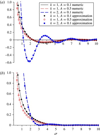
situation later. While it is possible to obtain more accurate approximations, these are accurate enough for our qualitative analysis. In figures 2(a) and 2(b), we give plots of the integrands (3.1) and (3.2) along with their approximations. The approximations are seen to be very accurate, provided that the helical filaments are of bounded variation (
 $Ak$
and
 $k$
sufficiently bounded). Even for the intermediate values used in the figures, the approximations are very accurate. Only when
 $A$
or
 $k$
become very large would we see any breakdown in the approximations. While the large-
 $A$
case is not particularly physical (since such solutions would be highly unstable, while we are considering solutions which persist in time, a priori, through the assumption (2.1)), it is possible to have large wavenumbers, and we discuss this case later.
Numerical plots and approximations to the integrand given in (a) (3.1) and (b) (3.2) for various values of the physical parameters. We set
 ${\it\epsilon}=10^{-5}$
in all plots. For small and intermediate values of
 $k$
and
 $A$
, the approximation to the integrand (3.1) is very accurate, and hence the approximating formula (3.7) for the integral term in (2.7) is accurate.

First, we have
 $$\begin{eqnarray}\displaystyle \int _{{\it\epsilon}}^{\infty }\frac{\cos (k{\it\sigma})-1+k{\it\sigma}\sin (k{\it\sigma})}{[{\it\sigma}^{2}+2A^{2}(1-\cos (k{\it\sigma}))]^{3/2}}\text{d}{\it\sigma}\! & {\approx} & \displaystyle \!\int _{{\it\epsilon}}^{\infty }\frac{\cos (k{\it\sigma})-1+k{\it\sigma}\sin (k{\it\sigma})}{(1+A^{2}k^{2})^{3/2}{\it\sigma}^{3}}\text{d}{\it\sigma}\nonumber\\ \displaystyle \! & = & \displaystyle \!\frac{\cos (k{\it\epsilon})-1+k{\it\epsilon}\sin (k{\it\epsilon})-k^{2}{\it\epsilon}^{2}\text{Ci}(k{\it\epsilon})}{2{\it\epsilon}^{2}(1+A^{2}k^{2})^{3/2}},\qquad\end{eqnarray}$$
where
 $\text{Ci}$
is the cosine integral
 $$\begin{eqnarray}\displaystyle \text{Ci}({\it\eta})=-\int _{{\it\eta}}^{\infty }\frac{\cos ({\it\sigma})}{{\it\sigma}}\text{d}{\it\sigma}. & & \displaystyle\end{eqnarray}$$
We find that
 $$\begin{eqnarray}\displaystyle \frac{\cos (k{\it\epsilon})-1+k{\it\epsilon}\sin (k{\it\epsilon})}{{\it\epsilon}^{2}}=\frac{k^{2}}{2}+O({\it\epsilon}^{2}) & & \displaystyle\end{eqnarray}$$
and
 $$\begin{eqnarray}\displaystyle \text{Ci}(k{\it\epsilon})={\it\gamma}+\ln (k)+\ln ({\it\epsilon})+O({\it\epsilon}^{2}). & & \displaystyle\end{eqnarray}$$
Therefore,
 $$\begin{eqnarray}\displaystyle & & \displaystyle \int _{{\it\epsilon}}^{\infty }\frac{\cos (k{\it\sigma})-1+k{\it\sigma}\sin (k{\it\sigma})}{[{\it\sigma}^{2}+2A^{2}(1-\cos (k{\it\sigma}))]^{3/2}}\text{d}{\it\sigma}\nonumber\\ \displaystyle & & \displaystyle \quad \approx -\frac{k^{2}}{2(1+A^{2}k^{2})^{3/2}}\left({\it\gamma}-\frac{1}{2}+\ln (k)+\ln ({\it\epsilon})\right)+O({\it\epsilon}^{2}).\end{eqnarray}$$
Here,
 ${\it\gamma}\approx 0.5772$
is the Euler–Mascheroni constant. We neglect terms of order
 ${\it\epsilon}^{2}$
and higher, since
 ${\it\epsilon}\ll 1$
. Returning to Ricca (Reference Ricca1994), this expression is similar to his equation (3.27) which was used when torsion tends to infinity. The difference is the dependence on the wavenumber, which is scaled out in Ricca (Reference Ricca1994). (More precisely, the results in Ricca Reference Ricca1994 involved scaling torsion,
 ${\it\tau}=k/(1+A^{2}k^{2})$
.) Keeping
 $k$
, we will be able to directly compare our results with the LIA. Ricca (Reference Ricca1994) obtained this integral in the limit
 ${\it\tau}\rightarrow \infty$
. For this to occur, the wavenumber must be large and
 $A$
must become small as
 $k$
becomes large. We do not consider this, since for finite
 $A$
the torsion will not be infinite. Rather, for finite
 $A>0$
, the torsion will attain a maximal value of
 ${\it\tau}=2A^{-1}$
at
 $k=A^{-1}$
. The
 ${\it\tau}\rightarrow \infty$
limit then corresponds to
 $A\rightarrow 0$
,
 $k\rightarrow \infty$
provided
 $Ak\rightarrow {\it\nu}$
, for
 ${\it\nu}<\infty$
. This is a very restrictive limit, since
 $A\rightarrow 0$
essentially gives us a line filament. What all of this means is that we should maintain the parameters
 $k$
and
 $A$
in our development, as opposed to scaling them out and taking any particular limit, in order to capture the behaviour of arbitrary helical filaments.
Regarding the second integral, we have
 $$\begin{eqnarray}\displaystyle \int _{{\it\epsilon}}^{\infty }\frac{1-\cos (k{\it\sigma})}{[{\it\sigma}^{2}+2A^{2}(1-\cos (k{\it\sigma}))]^{3/2}}\text{d}{\it\sigma}\! & {\approx} & \displaystyle \!\int _{{\it\epsilon}}^{\infty }\frac{1-\cos (k{\it\sigma})}{(1+A^{2}k^{2})^{3/2}{\it\sigma}^{3}}\text{d}{\it\sigma}\nonumber\\ \displaystyle \! & = & \displaystyle \!\frac{k{\it\epsilon}\sin (k{\it\epsilon})+1-\cos (k{\it\epsilon})}{2{\it\epsilon}^{2}}-\frac{k^{2}}{2}\text{Ci}(k{\it\epsilon}),\qquad\end{eqnarray}$$
and using
 $$\begin{eqnarray}\displaystyle \frac{k{\it\epsilon}\sin (k{\it\epsilon})+1-\cos (k{\it\epsilon})}{{\it\epsilon}^{2}}=\frac{3}{2}k^{2}+O({\it\epsilon}^{2}), & & \displaystyle\end{eqnarray}$$
we find
 $$\begin{eqnarray}\displaystyle & & \displaystyle \int _{{\it\epsilon}}^{\infty }\frac{1-\cos (k{\it\sigma})}{[{\it\sigma}^{2}+2A^{2}(1-\cos (k{\it\sigma}))]^{3/2}}\text{d}{\it\sigma}\nonumber\\ \displaystyle & & \displaystyle \quad \approx \frac{k^{2}}{2(1+A^{2}k^{2})^{3/2}}\left(\frac{3}{2}-{\it\gamma}-\ln (k)-\ln ({\it\epsilon})\right)+O({\it\epsilon}^{2}).\end{eqnarray}$$
Using the approximations (3.7) and (3.10) in (2.7) and (2.8), respectively, we have the approximations
 $$\begin{eqnarray}\displaystyle {\it\omega}_{\mathit{approx}}=-\frac{k^{2}(2{\it\gamma}-1+2\ln (k)+4\ln ({\it\epsilon}))}{(1+A^{2}k^{2})^{3/2}} & & \displaystyle\end{eqnarray}$$
and
 $$\begin{eqnarray}\displaystyle {\it\beta}_{\mathit{approx}}=\frac{A^{2}k^{3}(3-2{\it\gamma}-2\ln (k)-4\ln ({\it\epsilon}))}{(1+A^{2}k^{2})^{3/2}}. & & \displaystyle\end{eqnarray}$$
The curve describing the helical vortex filament, including non-local effects, is then given by the approximation
 $$\begin{eqnarray}\displaystyle \boldsymbol{r}(x,t) & {\approx} & \displaystyle \left\{x+\frac{A^{2}k^{3}(3-2{\it\gamma}-2\ln (k)-4\ln ({\it\epsilon}))}{(1+A^{2}k^{2})^{3/2}}t\right\}\boldsymbol{i}_{x}\nonumber\\ \displaystyle & & \displaystyle +\,A\cos \left(kx+\frac{k^{2}(2{\it\gamma}-1+2\ln (k)+4\ln ({\it\epsilon}))}{(1+A^{2}k^{2})^{3/2}}t+x_{0}\right)\boldsymbol{i}_{y}\nonumber\\ \displaystyle & & \displaystyle +\,A\sin \left(kx+\frac{k^{2}(2{\it\gamma}-1+2\ln (k)+4\ln ({\it\epsilon}))}{(1+A^{2}k^{2})^{3/2}}t+x_{0}\right)\boldsymbol{i}_{z}.\end{eqnarray}$$
If we are concerned with the representation (2.9) for the frame of reference translating with the filament, then
 ${\it\phi}_{\mathit{approx}}={\it\omega}_{\mathit{approx}}+k{\it\beta}_{\mathit{approx}}$
. Using the approximations (3.11), (3.12), we obtain
 $$\begin{eqnarray}\displaystyle {\it\phi}_{\mathit{approx}}=-\frac{(4\ln ({\it\epsilon})-3+2{\it\gamma}+2\ln (k))k^{2}}{\sqrt{1+A^{2}k^{2}}}-\frac{2k^{2}}{(1+A^{2}k^{2})^{3/2}}. & & \displaystyle\end{eqnarray}$$
The filament under representation (2.9) should then be approximated by
 $$\begin{eqnarray}\displaystyle & & \displaystyle \boldsymbol{r}(x,t)\approx X(t)\boldsymbol{i}_{x}\nonumber\\ \displaystyle & & \displaystyle \quad +\,A\cos \left(kX(t)+\left\{\frac{(4\ln ({\it\epsilon})-3+2{\it\gamma}+2\ln (k))k^{2}+2k^{2}(1+A^{2}k^{2})^{-1}}{\sqrt{1+A^{2}k^{2}}}\right\}t+x_{0}\right)\boldsymbol{i}_{y}\nonumber\\ \displaystyle & & \displaystyle \quad +\,A\sin \left(kX(t)+\left\{\frac{(4\ln ({\it\epsilon})-3+2{\it\gamma}+2\ln (k))k^{2}+2k^{2}(1+A^{2}k^{2})^{-1}}{\sqrt{1+A^{2}k^{2}}}\right\}t+x_{0}\right)\boldsymbol{i}_{z},\nonumber\\ \displaystyle & & \displaystyle\end{eqnarray}$$
where
 $$\begin{eqnarray}\displaystyle X(t)=x+\frac{A^{2}k^{3}(3-2{\it\gamma}-2\ln (k)-4\ln ({\it\epsilon}))}{(1+A^{2}k^{2})^{3/2}}t. & & \displaystyle\end{eqnarray}$$
4. Comparison with the core LIA and numerical approximations
If one were to strictly consider the LIA in the inner region, one would obtain (upon removing the integral terms from (2.2)–(2.4))
 $$\begin{eqnarray}\displaystyle {\it\omega}_{\mathit{LIA}}=-\frac{2\ln ({\it\epsilon})k^{2}}{(1+A^{2}k^{2})^{3/2}}>0\quad \text{and}\quad {\it\beta}_{\mathit{LIA}}=A^{2}k{\it\omega}_{\mathit{LIA}}=-\frac{2\ln ({\it\epsilon})A^{2}k^{3}}{(1+A^{2}k^{2})^{3/2}}>0. & & \displaystyle\end{eqnarray}$$
Under the LIA, the motion of a helical vortex filament then takes the form
 $$\begin{eqnarray}\displaystyle \boldsymbol{r}(x,t) & = & \displaystyle \left\{x-\frac{2\ln ({\it\epsilon})A^{2}k^{3}}{(1+A^{2}k^{2})^{3/2}}t\right\}\boldsymbol{i}_{x}+A\cos \left(kx+\frac{2\ln ({\it\epsilon})k^{2}}{(1+A^{2}k^{2})^{3/2}}t+x_{0}\right)\boldsymbol{i}_{y}\nonumber\\ \displaystyle & & \displaystyle +\;A\sin \left(kx+\frac{2\ln ({\it\epsilon})k^{2}}{(1+A^{2}k^{2})^{3/2}}t+x_{0}\right)\boldsymbol{i}_{z}.\end{eqnarray}$$
In terms of the parameters calculated through the LIA, we have that the approximations found for small and intermediate
 $k$
are
 $$\begin{eqnarray}\displaystyle {\it\omega}_{\mathit{approx}}=2{\it\omega}_{\mathit{LIA}}-\frac{k^{2}(2{\it\gamma}-1+2\ln (k))}{(1+A^{2}k^{2})^{3/2}} & & \displaystyle\end{eqnarray}$$
and
 $$\begin{eqnarray}\displaystyle {\it\beta}_{\mathit{approx}}=2{\it\beta}_{\mathit{LIA}}+\frac{A^{2}k^{3}(3-2{\it\gamma}-2\ln (k))}{(1+A^{2}k^{2})^{3/2}}. & & \displaystyle\end{eqnarray}$$
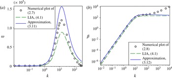
In figure 3, we plot these approximate solutions against both the inner LIA solutions and direct numerical integration of the integrals in (2.7), (2.8). For small and intermediate
 $k$
(
 $k$
of order unity or smaller), these approximations are in strong agreement with the numerical integrations. For larger
 $k$
, of order 10, the approximations tend to overestimate the numerical value of
 ${\it\beta}$
and
 ${\it\omega}$
slightly, whereas the inner LIA underestimates these values. The approximations are still more accurate than the inner LIA. For much larger
 $k$
, say of order
 $10^{2}$
and greater, both the approximation (3.11), (3.12) as well as the LIA lose their usefulness. This is due to the fact that the integral term has an integrand which rapidly oscillates for large
 $k$
.
Note that one could also approximate the outer region (which holds the non-locality) with another copy of the inner LIA, so that the total quantities are approximated by
 ${\it\beta}_{\ast }\approx 2{\it\beta}_{\mathit{LIA}}$
and
 ${\it\omega}_{\ast }\approx 2{\it\omega}_{\mathit{LIA}}$
. However, these approximations would overestimate
 ${\it\beta}$
and
 ${\it\omega}$
even more than
 ${\it\beta}_{\mathit{approx}}$
and
 ${\it\omega}_{\mathit{approx}}$
, particularly for intermediate or large values of
 $k$
. The qualitative behaviour of such an approximation would, of course, match that of the inner LIA alone.
Comparison of the numerical plots and approximate solutions for (a) the rotational velocity,
 ${\it\omega}$
, and (b) transverse velocity,
 ${\it\beta}$
, of a helical vortex filament when non-local dynamics are accounted for. The numerical results use the LIA near the logarithmic singularity, so these are the solutions (2.7) and (2.8), respectively. We set
 ${\it\epsilon}=10^{-5}$
in all plots. We also take
 $A=0.1$
. The analytical approximations obtained in (3.11), (3.12) are superior to the LIA (4.1) results when
 $k$
is either small or in the intermediate range. Once
 $k$
becomes large, both approximations lose accuracy. This is due to the fact that, for large
 $k$
, the integral terms in (2.7), (2.8) are rapidly oscillating. The approximations (3.11), (3.12) are useful when the decay in the integrals dominates the oscillations, which is not true for large
 $k$
. In the regime where the approximations are useful, note that the LIA underestimates both velocities, while the approximation (3.11), (3.12) overestimates the velocities.

From the plots, it is clear that there exists a critical value of the wavenumber for which the rotational velocity is maximal. In the approximation (3.11), (3.12), the LIA, and the numerical approximations, this value is nearly the same. Since the values are approximately the same, we use the LIA, finding that this critical wavenumber is given approximately by
 $k^{\ast }\approx \sqrt{2}A^{-1}$
. Note that this corresponds to the maximal value of torsion (since torsion
 ${\it\tau}$
is given by
 ${\it\tau}=k(1+A^{2}k^{2})^{-1}$
). So, the larger the torsion, the greater the rotational velocity. On the other hand, the plots indicate that the transverse velocity is always increasing, as mentioned when we considered the numerical results before.
In summary, the approximations (both LIA and those of (3.11), (3.12)) are accurate for small and intermediate
 $k$
(with the approximation (3.11), (3.12) being best), while there is a sharp breakdown in the approximations for larger
 $k$
in the case of transverse velocity (the approximations for the rotational velocity are always qualitatively correct). For both
 ${\it\omega}$
and
 ${\it\beta}$
, the breakdown for larger
 $k$
is due to the fact that the integrals oscillate rapidly. The primary qualitative difference is that the approximations fail to pick up the
 $O(k)$
growth in
 ${\it\beta}$
(although they nicely capture the
 $O(k^{2})$
for small
 $k$
). In the large-
 $k$
regime, this is in contrast to the LIA result, which suggests that the transverse velocity should tend to a constant value
 ${\it\beta}_{\mathit{LIA}}\rightarrow -(2\ln ({\it\epsilon})/A)$
as
 $k\rightarrow \infty$
. Since we keep
 $A>0$
, this value is always finite.
Let us revisit the frame of reference moving with the filament. Under the LIA, this gives the known dispersion relation
 $$\begin{eqnarray}\displaystyle {\it\phi}_{\mathit{LIA}}={\it\omega}_{\mathit{LIA}}+k{\it\beta}_{\mathit{LIA}}=-\frac{2\ln ({\it\epsilon})k^{2}(1+A^{2}k^{2})}{(1+A^{2}k^{2})^{3/2}}=-\frac{2\ln ({\it\epsilon})k^{2}}{\sqrt{1+A^{2}k^{2}}}. & & \displaystyle\end{eqnarray}$$
In the limit where
 ${\it\epsilon}$
is very small, the
 $\ln ({\it\epsilon})$
term in the expression (3.14) dominates, and we recover (using (4.5)) the relation which scales as
 ${\it\phi}_{\mathit{approx}}\sim 2{\it\phi}_{\mathit{LIA}}$
. For general
 ${\it\epsilon}>0$
, the relation is explicitly given by
 $$\begin{eqnarray}\displaystyle {\it\phi}_{\mathit{approx}}=2{\it\phi}_{\mathit{LIA}}+\frac{(3-2{\it\gamma}-2\ln (k))k^{2}}{\sqrt{1+A^{2}k^{2}}}-\frac{2k^{2}}{(1+A^{2}k^{2})^{3/2}}. & & \displaystyle\end{eqnarray}$$
5. The large-wavenumber limit
We were able to construct analytical approximations for the rotational and transverse velocities, in order to have a simpler qualitative approximation of the integral terms in
 ${\it\omega}$
and
 ${\it\beta}$
. These approximations were more accurate in the small and intermediate wavenumber regimes than the LIA. The approximations had a tendency to overestimate the velocities in these regimes (recall that the LIA underestimated the values). The primary failing of the analytical approximation is that it fails to pick up the proper growth rate for the translational velocity in the large-
 $k$
regime. The numerics show that for large
 $k$
, we should have
 ${\it\beta}\sim k$
. We can prove this analytically (even if we cannot obtain a closed-form approximation of
 ${\it\beta}$
in the large-
 $k$
limit). First, observe that
 $$\begin{eqnarray}\displaystyle 0<\int _{{\it\epsilon}}^{\infty }\frac{1-\cos (k{\it\sigma})}{[{\it\sigma}^{2}+2A^{2}(1-\cos (k{\it\sigma}))]^{3/2}}\text{d}{\it\sigma}<2\int _{{\it\epsilon}}^{\infty }\frac{\text{d}{\it\sigma}}{{\it\sigma}^{3}}=\frac{1}{{\it\epsilon}^{2}}. & & \displaystyle\end{eqnarray}$$
Since
 ${\it\epsilon}$
is chosen to be small yet positive, the integral must be finite, even as
 $k\rightarrow \infty$
. Therefore, the integral is a bounded function of
 $k$
. Returning to (2.8), we see that although the LIA term tends to zero as
 $k\rightarrow \infty$
, the integral is multiplied by a factor of
 $k$
, and since the integral is bounded and positive, the solution for
 ${\it\beta}$
must increase like a function of order
 $k$
as
 $k\rightarrow \infty$
. By a similar approach, one may show that
 ${\it\omega}$
must tend to a constant value as
 $k\rightarrow \infty$
, which is exactly what we see in figures 1 and 3.
In the asymptotic limit
 $k\rightarrow \infty$
(that is, the case where pitch is made to be small), the ratio of translational and rotational velocity should equal
 $A^{2}k$
as the helical vortex reduces to a cylindrical vortex sheet (Ricca Reference Ricca1994). For the LIA we have
 $$\begin{eqnarray}\displaystyle \frac{{\it\beta}_{\mathit{LIA}}}{{\it\omega}_{\mathit{LIA}}}=A^{2}k, & & \displaystyle\end{eqnarray}$$
hence this is always true. Let us consider the approximations (3.11) and (3.12), which give
 $$\begin{eqnarray}\displaystyle \frac{{\it\beta}_{\mathit{approx}}}{{\it\omega}_{\mathit{approx}}}=A^{2}k\left(\frac{3-2{\it\gamma}-2\ln (k)-4\ln ({\it\epsilon})}{1-2{\it\gamma}-2\ln (k)-4\ln ({\it\epsilon})}\right). & & \displaystyle\end{eqnarray}$$
In the double limit
 ${\it\epsilon}\rightarrow 0$
,
 $k\rightarrow \infty$
we have
 $$\begin{eqnarray}\displaystyle \lim _{k\rightarrow \infty }\lim _{{\it\epsilon}\rightarrow 0}\frac{3-2{\it\gamma}-2\ln (k)-4\ln ({\it\epsilon})}{1-2{\it\gamma}-2\ln (k)-4\ln ({\it\epsilon})}=\lim _{k\rightarrow \infty }\lim _{{\it\epsilon}\rightarrow 0}\frac{-2\ln (k)-4\ln ({\it\epsilon})}{-2\ln (k)-4\ln ({\it\epsilon})}=1. & & \displaystyle\end{eqnarray}$$
Therefore, we have the scaling
 $$\begin{eqnarray}\displaystyle \frac{{\it\beta}_{\mathit{approx}}}{{\it\omega}_{\mathit{approx}}}\sim A^{2}k & & \displaystyle\end{eqnarray}$$
in the large-
 $k$
limit. In the case of the approximations obtained for the Biot–Savart integrals, the required result still holds. This is good, since it means that the approximations still give qualitatively reasonable results for large
 $k$
.
Regarding the actual integrals, let us define the integral in the
 ${\it\omega}$
solution (2.7) by
 $I_{{\it\epsilon}}(A,k)$
and the integral in the
 ${\it\beta}$
solution (2.8) by
 $J_{{\it\epsilon}}(A,k)$
. That is
 $$\begin{eqnarray}\displaystyle I_{{\it\epsilon}}(A,k)=\int _{{\it\epsilon}}^{\infty }\frac{\cos (k{\it\sigma})-1+k{\it\sigma}\sin (k{\it\sigma})}{[{\it\sigma}^{2}+2A^{2}(1-\cos (k{\it\sigma}))]^{3/2}}\text{d}{\it\sigma} & & \displaystyle\end{eqnarray}$$
and
 $$\begin{eqnarray}\displaystyle J_{{\it\epsilon}}(A,k)=\int _{{\it\epsilon}}^{\infty }\frac{1-\cos (k{\it\sigma})}{[{\it\sigma}^{2}+2A^{2}(1-\cos (k{\it\sigma}))]^{3/2}}\text{d}{\it\sigma}. & & \displaystyle\end{eqnarray}$$
Under a change of variable
 $m=k{\it\sigma}$
, we can write
 $I_{{\it\epsilon}}(A,k)=k^{2}{\hat{I}}_{{\it\epsilon}}(A,k)$
and
 $J_{{\it\epsilon}}(A,k)=k^{2}{\hat{J}}_{{\it\epsilon}}(A,k)$
, where
 $$\begin{eqnarray}\displaystyle {\hat{I}}_{{\it\epsilon}}(A,k)=\int _{{\it\epsilon}k}^{\infty }\frac{\cos (m)-1+m\sin (m)}{[m^{2}+2A^{2}k^{2}(1-\cos (m))]^{3/2}}\text{d}m & & \displaystyle\end{eqnarray}$$
and
 $$\begin{eqnarray}\displaystyle {\hat{J}}_{{\it\epsilon}}(A,k)=\int _{{\it\epsilon}k}^{\infty }\frac{1-\cos (m)}{[m^{2}+2A^{2}k^{2}(1-\cos (m))]^{3/2}}\text{d}m. & & \displaystyle\end{eqnarray}$$
We may therefore express the ratio
 ${\it\beta}/{\it\omega}$
for the solutions (2.7), (2.8) by
 $$\begin{eqnarray}\displaystyle \frac{{\it\beta}}{{\it\omega}}=A^{2}k\left(\frac{M(A,k)+4{\hat{J}}_{{\it\epsilon}}(A,k)}{M(A,k)+4{\hat{I}}_{{\it\epsilon}}(A,k)}\right), & & \displaystyle\end{eqnarray}$$
where
 $M(A,k)$
denotes the term present under the LIA. For the pure LIA case, we do not have the
 ${\hat{I}}$
or
 ${\hat{J}}$
terms and hence this ratio is always
 $A^{2}k$
. We would like to show that the
 ${\hat{I}}$
and
 ${\hat{J}}$
terms vanish in the
 $k\rightarrow \infty$
limit, so that we recover the LIA result in this limit. Observe that
 $$\begin{eqnarray}\displaystyle |{\hat{I}}_{{\it\epsilon}}(A,k)| & {\leqslant} & \displaystyle \int _{{\it\epsilon}k}^{\infty }\frac{|\!\cos (m)-1+m\sin (m)|}{[m^{2}+2A^{2}k^{2}(1-\cos (m))]^{3/2}}\text{d}m\nonumber\\ \displaystyle & {\leqslant} & \displaystyle \int _{{\it\epsilon}k}^{\infty }\frac{m+2}{[m^{2}+4A^{2}k^{2}]^{3/2}}\text{d}m\leqslant \int _{{\it\epsilon}k}^{\infty }\frac{m+2}{m^{3}}\text{d}m=\frac{1+{\it\epsilon}k}{{\it\epsilon}^{2}k^{2}},\end{eqnarray}$$
 ${\hat{I}}_{{\it\epsilon}}(A,k)\rightarrow 0$
as
 $k\rightarrow \infty$
for any fixed finite
 ${\it\epsilon}>0$
. Similarly,
 $$\begin{eqnarray}\displaystyle |{\hat{J}}_{{\it\epsilon}}(A,k)| & {\leqslant} & \displaystyle \int _{{\it\epsilon}k}^{\infty }\frac{|1-\cos (m)|}{[m^{2}+2A^{2}k^{2}(1-\cos (m))]^{3/2}}\text{d}m\nonumber\\ \displaystyle & {\leqslant} & \displaystyle \int _{{\it\epsilon}k}^{\infty }\frac{2}{[m^{2}+4A^{2}k^{2}]^{3/2}}\text{d}m\leqslant \int _{{\it\epsilon}k}^{\infty }\frac{2}{m^{3}}\text{d}m=\frac{1}{{\it\epsilon}^{2}k^{2}},\end{eqnarray}$$
 ${\hat{J}}_{{\it\epsilon}}(A,k)\rightarrow 0$
as
 $k\rightarrow \infty$
for any fixed finite
 ${\it\epsilon}>0$
. These are crude estimates, and the actual values are probably much smaller (perhaps orders of magnitude smaller in
 $k$
). However, this shows that the
 ${\hat{I}}$
and
 ${\hat{J}}$
terms vanish in the
 $k\rightarrow \infty$
limit, and therefore the solutions (2.7), (2.8) satisfy
 ${\it\beta}/{\it\omega}\rightarrow A^{2}k$
in the large-
 $k$
limit. Therefore, the ratio of translational and rotational velocity under the solutions (2.7), (2.8) does equal
 $A^{2}k$
, and the helical vortex reduces to a cylindrical vortex sheet in the non-local solutions as well as for the LIA. Therefore, in the
 $k\rightarrow \infty$
limit, these results agree with those of Ricca (Reference Ricca1994) for the small-pitch limit.
6. Conclusions
By studying the helical vortex filament in Cartesian coordinates under the non-local Biot–Savart formulation with the approximation approach used here, we have been able to compare our solutions directly with those corresponding to the LIA. The LIA itself is commonly employed in order to study vortex filament dynamics, since it permits much simpler solutions. We have seen that the LIA solutions generally underestimate both the rotational and transverse velocity of helical vortex filaments. Physically, this means that the non-local effects due to the Biot–Savart formulation result in faster helical Kelvin waves or perturbations along a line filament. From plotting the numerical profiles for both velocities, we observe that the rotational velocity is maximal at a specific wavenumber which corresponds to the maximal torsion, which makes complete sense and is in agreement with findings of Ricca (Reference Ricca1994). Since we allow solutions in the intermediate amplitude and wavenumber regime, the torsion is always bounded. In the limit where the radius
 $A$
of the helix goes to zero, the torsion tends to infinity, and one obtains the analytical results of Ricca (Reference Ricca1994). That case would correspond to the limit where the helical filament decays into a line filament. Regarding the translational velocity of helical waves along the filament, we see that the helical waves propagate at an increasing rate along the filament as the wavenumber increases, which is to be expected. However, the translational velocity is not monotone with the wavenumber. Rather, the translational velocity scales like
 $k^{2}$
when
 $k$
is small, and like
 $k$
when
 $k$
is large. The behaviour of
 ${\it\beta}$
and
 ${\it\omega}$
is in qualitative agreement with the
 $O(1)$
numerical results of figure 3 in Widnall (Reference Widnall1972), if one notes that
 ${\it\alpha}$
is the pitch (which itself is a function of the wavenumber) in that paper, and therefore there exists a critical value of the pitch at which the rotational velocity is maximal while for all values of pitch the translational velocity is monotone.
It is worth mentioning that there is a quantum form of the LIA, which is essentially the LIA applied to the HVBK model (Hall & Vinen Reference Hall and Vinen1956a
,Reference Hall and Vinen
b
; Bekarevich & Khalatnikov Reference Bekarevich and Khalatnikov1961). It should be feasible to extend the present analytical results to that model or one of its potential forms (Van Gorder Reference Van Gorder2014a
), at least in the case of helical filaments with constant amplitude
 $A$
. The exact form of a helical filament under the quantum LIA, including decay, was discussed in Van Gorder (Reference Van Gorder2014b
). In the case of decaying filaments (
 $A=A(t)$
such that
 $A\rightarrow 0$
as
 $t\rightarrow \infty$
), the non-local development may be possible analytically, but will be much more complicated.
Acknowledgements
The author was supported in part by NSF grant number #1144246. The author wishes to thank the anonymous referees, whose comments have led to definite improvement in the presentation of the results.