

1. INTRODUCTION
The notion of a scientific “network” has played an increasingly important and prominent role in both empirical and theoretical studies of the development and (especially) dissemination of scientific knowledge. Such networks are defined variously, with the nodes occupied by scientists, institutions (such as labs), scientific papers, etc., and the links given by collaboration, communication, citation, etc. Such networks are prima facie relevant to the analysis of the production and dissemination of scientific knowledge (itself defined variously), though the flexibility in how they are defined does raise the danger that we will find what we are looking for (e.g., “the importance of networks in science”), no matter what we are looking for.Footnote 1
Despite this danger, their is indeed ample evidence (both empirical and theoretical) that more or less stable networks of scientists, laboratories, and other resources, play a significant role in the production of scientific knowledge (see note 1 for a very few references among the hundreds out there). Often this role is found to be – and sometimes it is presumed to be – positive, in the sense of enhancing, in one way or another, the production or dissemination of scientific knowledge. But isthis influence always positive in that sense? It is not difficult to imagine that networks might also be barriers of one sort or another. What would happen if there were no networks to speak of? What would happen, for example, if scientists could not even remember one another from one moment to the next?
It sounds like a recipe for chaos – no stable social structure, just scientists developing and shouting their theories to one another. The point of this short paper is to explore what – at least in a simple model – would, indeed, happen if the scientificworld were chaotic in this way. The point of the exercise is not, of course, to provide a model of actual scientific practice. It is, rather, to sound a cautionary note: Despite the (correct) emphasis on the role of networks of various kinds in studies of the development and dissemination of scientific knowledge, we should bear in mind that the simple fact that scientists have a common goal – the development and dissemination of knowledge about the world – goes a long way towards explaining the emergence of widely held scientific theories. For as we shall see, at least in the model discussed below, theory does indeed emerge from scientific chaos.
In the next section I will describe how the model works for a single theorizer. In the subsequent section, I will describe the chaotic world of many such theorizers, the sense in which I take it to be “networkless,” and what emerges in the model under simulation.Footnote 2 It may be tempting to think of the next section as concerned with “development” and the following one as concerned with “dissemination,” but this way of thinking is misleading. Although the single theorizer mentioned in the next section can indeed “develop” a scientific theory (in the sense described there), once we introduce several such theorizers, development and dissemination become entangled. This entanglement is actually quite important for the widespread (but not universal) agreement amongst theorizers in the model. Were they to develop and then disseminate, there would be no agreement (apart from accidental agreement).Footnote 3
2. THEORIZING
This section develops the idea of a “theorizer,” modeled as playing a “prediction game.” Learning to make good predictions about a law-like (but stochastic) world is likened to developing a scientific theory. The model is extremely simplistic, but does contain some important ingredients of scientific theorizing, or so it is claimed.
2.1 Prediction games
Recent work on signaling games has demonstrated that they can be used to model a number of phenomena conceived as “signaling systems,” far beyond Lewis' (Reference Lewis1969) original target of successful communication via conventionally defined terms.Footnote 4 Following Barrett, Dickson, and Purves (in preparation), I use a more general form of such games (“prediction games”) to model scientific theorizing, albeit in a very rudimentary way.
In a simple iterated signaling game there are N states (sometimes referred to as states of the world, sometimes as types of the first player), chosen randomly (typically from a stationary, often flat, distribution) in each round of the game. The first player (“sender”) produces a “signal” chosen from a set of S many potential signals according to a distribution determined by the state. The second player (“receiver”) then performs an “act” chosen from a set of A many potential acts according to a distribution determined by the signal. (The game is thus one of asymmetric information.) Signals and acts are determined by “dispositions,” which are sets of N many (for sender) or S many (for receiver) probability distributions over the signals (for sender) or acts (for receiver). These distributions are typically taken to be initially flat. There is a utility measure over states, signals, and acts for both sender and receiver. (Typically one presumes that N = S = A but this assumption can be relaxed. In some games, in fact, these numbers may be dynamic. In the model here, I've kept things simple: N = S = A.)
Lewisian signaling games are cooperative (i.e., the agents' utilities are aligned). This fact is reflected in how the agents in the game learn (adapt). After each round, if the payoff to sender and receiver is positive, then both receiver and sender are reinforced, meaning that their distributions are modified so that they are more likely to repeat their respective “outputs” (signal for sender, act for receiver) under the same “inputs” (state of the world for sender, signal for receiver). They may alsobe negatively reinforced if their payoffs are negative.
This reinforcement is implemented by representing each player's probability distributions as sets of “propensities,” each propensity being a positive integer. On positive reinforcement, the size of the propensity corresponding to the performed action (the input and output) is increased by 1 (or some other fixed number). Probabilities are determined from these propensities in the obvious way (divide the propensity for the output in question by the sum of all propensities for the given input). This algorithm is familiar as the “basic model” used by Roth and Erev (Reference Roth and Erev1995), who discuss its pedigree and relation to evolutionary dynamics. I refer to the matrix of probabilities and the matrix of propensities from which they are derived indifferently as the player's “disposition.” Similarly, on failure, propensities may be decreased. In this case, one must define what happens when a propensity would go to zero. In the model below, propensities have a minimum value of 1, which means that, in principle, all outputs are always at least possible for any input.
In addition to adding such penalties to the basic learning algorithm, one may consider further dynamical modifications to agents' dispositions. Here I adopt just one, which corresponds closely to what Roth and Erev (Reference Roth and Erev1995) call “gradual forgetting.”Footnote 5 Gradual forgetting is in essence the imposition of a maximum size for the propensities. Doing so ensures that even after a long time, present success or failure effects dispositions about the same as medium-term successes or failures did.Footnote 6 (On the other hand, early successes and failures still have a much larger influence on dispositions. This situation is desirable, because it means that the “learning curve” is very steep in the early stages of the game, allowing agents very quickly to evolve successful dispositions.)Footnote 7 Here I implement forgetting by multiplying each propensity by a factor, ϕ, every F rounds of the game,Footnote 8 where 0 < ϕ≤ 1, with equality on the right if there is no forgetting. Forgetfulness can improve success by giving agents who early on evolved towards unsuccessful strategies a chance to change direction. Without forgetfulness, the size of the propensities can grow so large that before long, even a long string of failures cannot affect the agent's disposition appreciably. (The fact that agents often evolve successful signaling systems even with ϕ = 1 is a testament to the rarity of evolving “badly” in the early stages.)
Under a wide range of choices for the size of reward, penalty, and forgetting, and with relatively small values for N, S, and A, agents in simulation typically evolve successful signaling systems, where “success” is defined in the next subsection. This phenomenon has been much studied, including under a wide range of modifications of the basic Lewisian game (see, e.g., the references in note 1).
In prediction games, the following modification is made: the state of the world evolves in some law-like manner, and agents are rewarded if the receiver's act matches not the current, but the next state of the world. The reward occurs once the next state of the world occurs.
Many of the phenomena modeled by signaling games are indeed of this sort already. For example, signaling games have been used to model alarm calls (see, e.g., Zollman et al. Reference Zollman, Bergstrom and Huttegger2013 and references therein), which can be understood as an indication of the present state of the world, the importance of which, however, lies in what future states it could lead to. Similarly, signals used to find or keep mates may be understood as signals about present fitness, but again the importance of that present state is felt only in the future (for example, as the outcome of a fight).
There are of course many ways to introduce law-like evolution. A simple and obvious one would be to let the state move to the “next” one (i.e., a state of n = 3 on round t goes to n = 4 on round t + 1). In this case, I say that there is a “drift” of 1. (In such a dynamic, when n = N then on the next round it cycles back to n = 1, and in general we mod the drifted state by N.) This deterministic case is in fact no different from a signaling game, which is no surprise given the point made in the previous paragraph. However, it is arguably the case that this deterministic prediction game does not really get at the notion of “prediction.” After all, the sender's signal could be taken as a direct indication of how to act, rather than as a statement about how the world is now, which would then be used by receiver to make a prediction. (As we will see below, the correct understanding of prediction games – and arguably prediction itself! – is actually neither of those given in the previous sentence.)
So, in order to get at the notion of prediction, we must introduce some randomness into the model. Here it is done so in the form of a standard deviation. Hence, in the dynamics of this model, the next state of the world is chosen by allowing the current state to drift by some specified (and constant) amount, and then the actual next state is chosen from a normal distribution centered at the drifted state, with some specified (and constant) standard deviation.
This model is indeed more like learning in the real world, even when what is being learned is, at bottom, deterministic in nature. For it is a rare case where agents are able to home in on exactly which features of the current state of the world allow for deterministic prediction of the next state of the world. Unavoidable randomness in the real, messy, world, thus complicates learning in a way that is reflected, at least in a rudimentary way, in prediction games. Sometimes the predator just walks on by. Sometimes the underdog wins the fight. In a prediction game with randomness, the sender and receiver are forced to home in on the underlying “drift” in the face of the randomness presented by the standard deviation of the dynamics.
2.2 Measures of success
What do we mean by “success”? There are (at least) three questions that we might ask about sender-receiver pairs evolving according to the dynamics given above.Footnote 9
First (“stability”): How quickly (if ever) do they become “stable,” i.e., their dispositions no longer change much over time? To address this question, one can measure the evolving “differences” between the agent's dispositions at different times in terms of the mean Kullback-Liebler (KL) divergence (the relative entropy) between the agent's probability distributions (one for each possible input) at various intervals (for example, every 100 rounds). When these differences begin to change vary little, we may say that the agents are “stable”. In practice, “stability” entails that the agent is extremely unlikely to change its disposition appreciably in the future.
Second (“accuracy”): How well do a pair's dispositions get the receiver's act to match the next state of the world? And how does this accuracy evolve as the players' dispositions evolve? It is a simple matter to calculate the overall probability that a pair will be successful on any given round of the game. It is important of course, to take account of differences in the relative frequency with which a given state appears, in the long run. A simple way to avoid that issue is to choose a drift term that guarantees that states will be visited with equal relative frequency, in the long run.
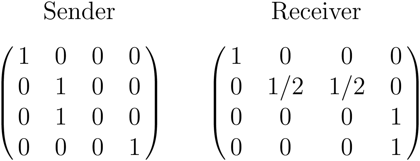
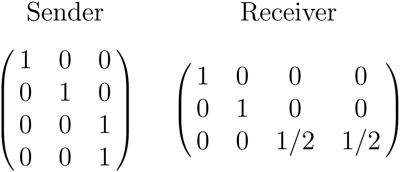
Third (“efficiency”): How efficiently does a pair make use of its available signals? One natural understanding of “efficiency” is that a pair is (fully) efficient if and only if it does the best it can to associate, deterministically, to each act of receiver, a state of the world. Consider, as an example of inefficiency, the partial pooling equilibrium in Fig. 1. In that case, sender and receiver are not making effective use of an available signal (signal 3). One might contrast this case with one in which there are four states of the world, but the pair has only three signals. They could, in that case, evolve dispositions that look like partial pooling, as in Fig. 2. But in fact the pair represented in Fig. 2 is “doing the best it can” given its limited resources. Without going into further mathematical details, I will present measures of efficiency as percentages, which should be understood as a measure of the extent to which the pair is “doing the best it can.” Hence, for example, the pair in Fig. 1 is 75% efficient, while the pair in Fig. 2 is 100% efficient.Footnote 10
A partial pooling equilibrium.

A partial pooling equilibrium.
For relatively small values of N, S, and A, under a wide variety of choices for values of the other parameters of the model (reward, penalty, forgetfulness, drift, standard deviation, and others either implied above or not introduced here and not used in the models described here), prediction pairs develop quite successful prediction systems. For example,Footnote 11 with N = S = A = 4, a drift of 1, standard deviation of 0.5, and reasonable choices for the other parameters of the model, Barrett, Dickson, and Purves (in preparation) report that out of 10,000 pairs, 88% were stable at the time that the simulation was ended,Footnote 12 overall accuracy was 94%,Footnote 13 and overall efficiency was 95%.Footnote 14 Agents began to stabilize after around 5,000 rounds, though the simulation was run to 20,000 rounds in that case.
2.3 Prediction pairs as theorizers
I think of a given pair in a prediction game as a “theorizer,” and the “agents” in the model described in the next section consist of such pairs (i.e., each agent is a theorizer). The idea is that theorizing has (at least) two (intertwined) components: representation and prediction. A given pair is in fact learning to do both.
It is tempting to think of the sender as the “representer” and the receiver as the “predictor,” but, as noted above, this way of thinking about what is happening is wrong, and a moment's reflection on the notion of representation (and perhaps more than a moment on the notion of prediction) may reveal why, but here I will just note that the incorrectness of this way of thinking is especially apparent when a theorizer is presented with a change in the laws. In this case, one might think that the “representer” (sender) maintains its disposition while the “predictor” (receiver) changes to accommodate the new laws.
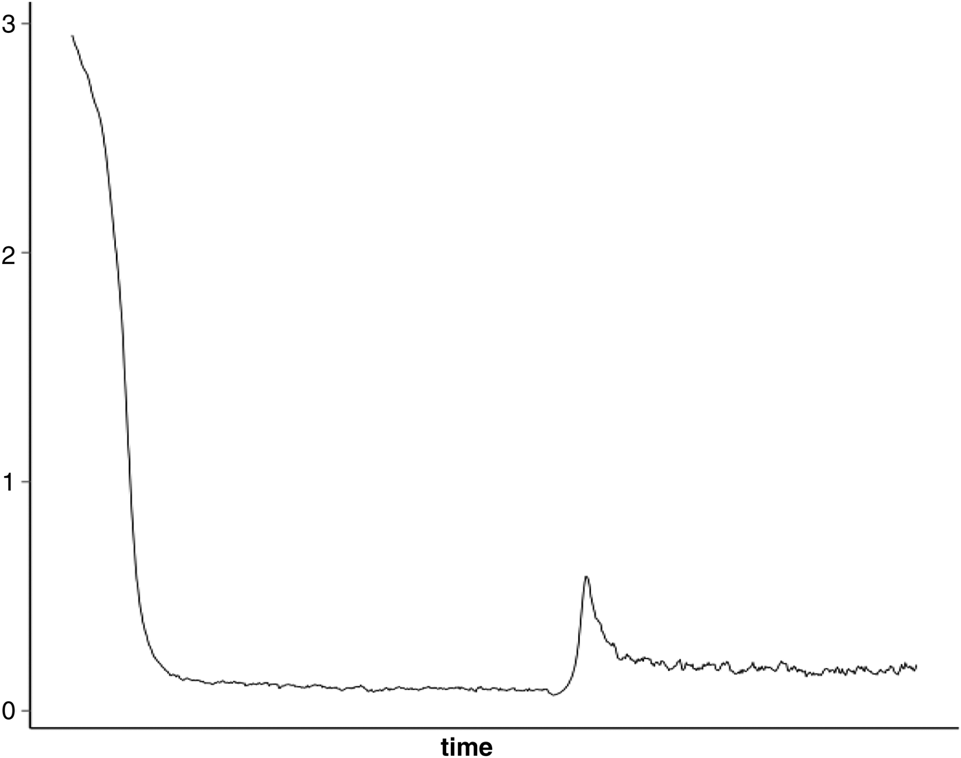
In fact, however, the two change in a more holistic manner. In general, as Barrett, Dickson, and Purves (in preparation) report, each member of a pair will tend to hold on to some parts of its old disposition and change others. Indeed, precisely because of this phenomenon, they tend to learn the new laws more quickly than they learned the old ones – they have some “representational” and “predictive” resources that they can immediately put to use when learning the new laws, whereas they started learning the old laws with absolutely nothing (i.e., all flat distributions). That they do so (i.e., that they do not start relearning from scratch) is evident in the data represented by Fig. 3. The scenario in this case was that the simulation was run (on 10,000 theorizers) with a drift of 1 (and standard deviation of 0.5). Then, once most pairs had settled on a prediction system (i.e., they became stable), the laws were changed (drift became 3). What we see in the graph is the mean across all theorizers of the mean (across all 8 distributions for “sender” and all 8 distributions for “receiver”) KL-divergence from a completely settled (efficient) prediction system (the one closest to their current, possibly unstable, system).Footnote 15
Mean KL-divergence from an established prediction system in a scenario where the laws were changed part way through the simulation (in this case, N = S = A = 8). The graph never reaches the bottom mainly because of the existence of partial pooling equilibira. The simulation was run to 80,000 rounds, total.
The point at the top left of the graph represents the case where all agents are as “far” as possible (in the sense of KL-divergence) from an efficient prediction system. As the graph moves lower, the agents are, on average, beginning to favor given outputs for given inputs, and near the bottom, they are, on average, very close to a completely efficient system, i.e., one in which sender's signal carries as much information as possible about the state of the world and receiver's act carries as much information as possible about the signal that it received. It is important to bear in mind that what is being represented by “mean KL-divergence from an established prediction system” is the “distance” (in the sense of KL-divergence) that a pair is from the nearest efficient system to its own, actual, system, and not from an optimal system.Footnote 16 In the latter case, the graph in 3 would make no sense, because we would be comparing pairs to two different (optimal) systems, before and then after the point when the laws changed. To put it another way, we are measuring distance from efficiency, not distance from optimality – efficient systems represent firm beliefs, while optimal systems represent firm true beliefs.
Note that while the theorizers do become somewhat unsettled (i.e., they begin to act in a less predictable way, at least for some inputs), they do not simply “forget” everything that they learned – that is, they do not return to the flat dispositions with which they began. Therefore, their (albeit, at this stage, non-deterministic) tendencies that are “left over” from the previously efficient disposition has an influence on how they learn the new laws. Examination of the evolution of individual theorizers as they learn the new laws confirms that each of “sender” and “receiver” hold on to some aspects of their previous disposition, in general. (In other words, repeated runs of the simulation results in graphs substantially similar to that in 3.)
However, this “conservatism” can also have a negative effect on their ability to relearn, and this point will become important below. In standard prediction games, especially as N, S, and A get large, theorizers will typically not learn the new laws quite as well as they learned the old ones. This fact is reflected, for example, in Fig. 4, which shows the stability, efficiency, and accuracy for the same simulation represented in Fig. 3. Note that the agents “restabilize” at a level of accuracy (86.5%) and efficiency (89.8%) slightly below where they were after first stabilizing (90.7% and 92.1%, respectively). This phenomenon, too, is very robust. I will return to this point later.
(colour online) Stability accuracy, and efficiency from the same simulation represented in Fig. 3. The line for accuracy begins at 12.5% and is the first to rise. The lines for efficiency and stability both begin at zero, and the first of these to rise is efficiency.
3. CHAOS
3.1 The model
The model of “chaotic science” consists of a collection of theorizers, placed on a grid. This grid may be taken to represent “communicative distance,” in the sense that one agent can (but need not) communicate with other “nearby” agents, but not with far-away agents. Agents may be permitted to move about the grid, or not. Agents may “choose” to “broadcast” information, and may “choose” to “listen” to other agents in a variety of ways or under a variety of conditions.
It would, of course, be a simple matter to build “networks” into this structure. For example, one might predefine certain groups of agents to constitute networks. Or one might allow them to be established by considering that two agents become linked into a network once they have communicated, in some fashion, some number of times, or perhaps only if there have been some number of “successful” communications (however one might wish to define “success”). And so on.
However, as indicated above, the point of the model, here, is to explore what happens when agents do not really have the resources to form networks. So, in particular, the agents in this model have no way of identifying one another from one round of the game to the next. Hence, in particular, there are no links among agents that could be taken to define a network. Indeed, agents in this model (i.e., theorizers modeled as sender-receiver pairs playing a prediction game) have exactly and only the resources described in the previous section.
There is a perfectly clear sense in which the agents in such a model constitute a “network” of sorts, simply in virtue of the spatial relations among them and the (potential) communication that those spatial relations may enable (or prevent). Hence it is a bit of a stretch to say, as I did earlier, that the model is “networkless.” However, this “network” differs significantly from the sorts of network to which I referred in the introduction. The difference is most easily noticed in light of the fact that agents in this model have no capacity to recognize or remember one another. Hence, for example, they cannot establish a “reputation,” or a “record of success” (at least, not one that can be recognized by any agent); nor can they “agree” to work together (collaborate, share resources). Indeed, there is no straightforward sense in which agents can recall whether they listened to another agent on any previous round, and a fortiori whether any such case of listening was successful. So if one wishes to think of the model here as belonging to the general class of network-based models of the development and dissemination of scientific knowledge, one may do so, bearing in mind, however, that the notions in terms of which such models are typically defined (reputation, trust, long-term or medium-collaboration, etc.) are not available, here.
In defining a specific version of the very general model described above, there are several issues to settle, and in each case, there are numerous options, not difficult to imagine. Here I simply describe the options that I used, which were chosen to see what emerges when, in some appropriate sense, the model has “as little network structure as possible” while still containing enough potential for interaction among agents to make some sort of agreement (beyond what would be expected statistically) at least possible.
Immediately after choosing (but not yet sending or performing) a “signal” (or “representation”) and an “act” (or “prediction”), agents always broadcast which signal they have chosen, and which act they have chosen. They also broadcast their degree of confidence in these choices (as given by the strength of their propensities, expressed as probabilities – so a very strong propensity (high probability) to produce a given output is taken to indicate a high degree of confidence in that output). This information is broadcast to some portion of the “world” given by a radius (a definable parameter of the model) around the agent. Agents can “hear” any broadcast that reaches them. If their own level of confidence is below a threshold (a definable parameter of the model) then they “choose” a randomly selected broadcast (from among those that reach them), and if the level of confidence in the broadcast is above a threshold (another definable parameter in the model), the agent will choose the outputs given by the broadcast instead of those it had previously, provisionally, chosen. Everything else proceeds as before. At the end of each round, agents move a random distance (including possibly zero, up to a maximum that is a parameter of the model), in a randomly chosen direction.
In the models explored for present purposes, broadcast radius is small (less than 5% of the area of the world), the threshold to possibly listen to a broadcast is 80%, and the confidence in the broadcast must be no less than 80% in order for an agentto listen to it. In addition, agents move slowly – on each round they have a 1% chance to move one cell (in a randomly chosen direction). Finally, the world is fixed at 80 × 80 cells, and there are 100 agents.
These choices for the parameters are meant to reflect the kind of science described earlier. Agents frequently do not listen to one another and almost never in the crucial early stages of theorizing. And bear in mind that they do not recall from one round to the next to whom they listened (if anybody) or even whether they did. So a single instance of listening to another agent – even if it led to success – is far less than what it would take, for example, to create much likelihood that their propensities would move in the direction of those of the agent to whom they listened. Agents are quite unlikely to encounter all other agents even after many thousands of rounds of the game. I will quantify a few of these remarks below. For now, the point is that the way we have set things up, anything that looks like cooperation and agreement is far from guaranteed by the model.
3.2. Results
Under a wide range of values for the various parameters of the model, as in the case of a simple prediction game, the theorizers develop a successful system of prediction. Consider the case of N = S = A = 8 with a drift of 1 and standard deviation of 0.5 (as in the results reported above for prediction games). Then the theorizers develop a prediction system with an average accuracy and efficiency of around 95%.
By itself, this result might already seem surprising. After all, it would seem that in the course of developing one's own prediction system, listening to another (who will, in general, be developing an incompatible prediction system) could easily make it more difficult to converge to a successful system. However, in general, we find that instead theorizers develop slightly better systems when they are in this environment, compared with working entirely alone.
But perhaps more surprising is that the theorizers develop mostly the same system – that is, they (mostly) have the same “theory” (the same dispositions). In short, quite minimal, random, episodic, communication leads to a (mostly) unified theory.
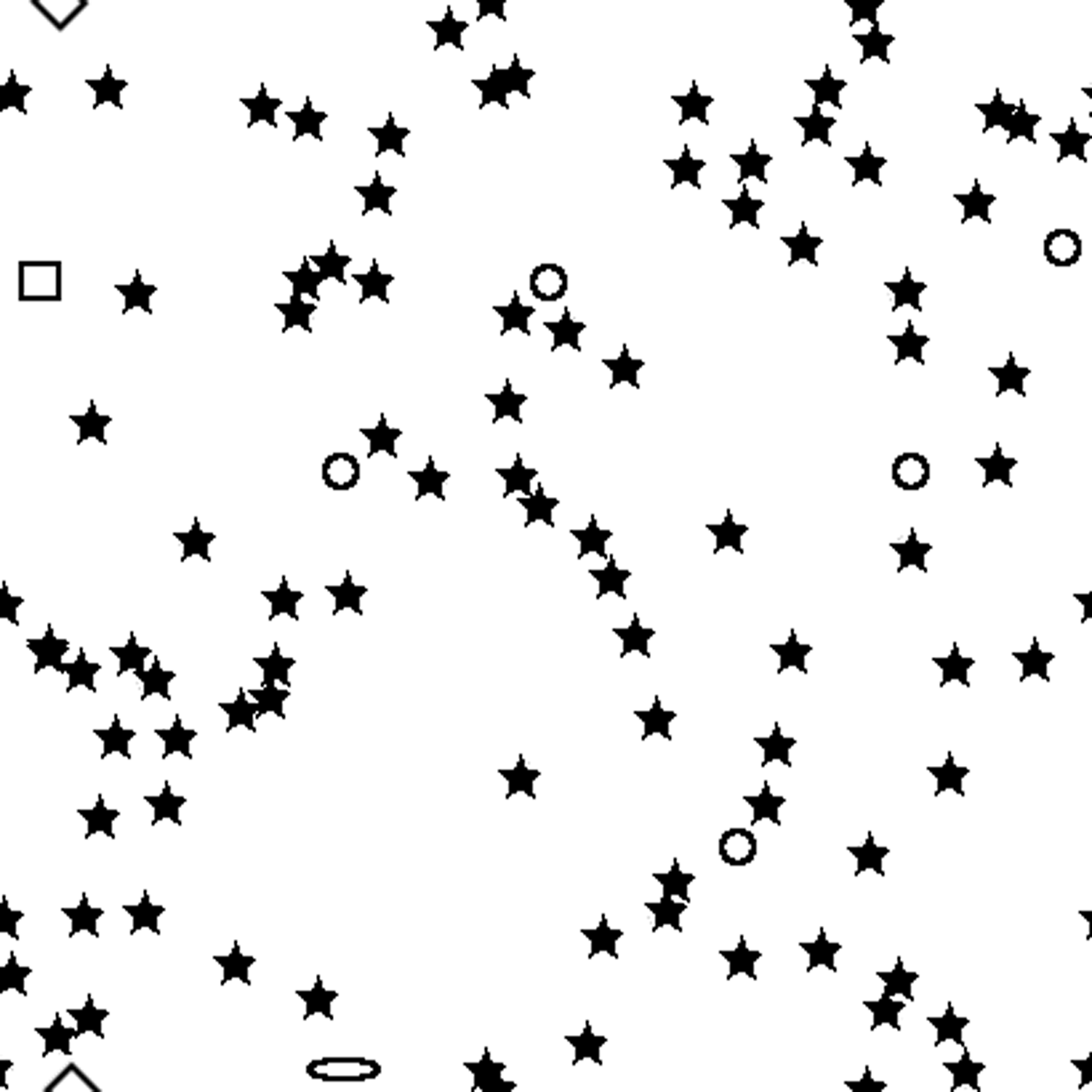
However, there are always (well, in every simulation that I have run) holdouts,Footnote 17 in the sense that a few theorizers will develop an alternative theory, which remains stable over time. For example, in 100 runs of the simulation described above, on average 6.6 of the 100 theorizers developed a theory different from the majority view (i.e., the picture shown in Fig. 5, which represents a single run, is typical).
Chaotic science has become widespread agreement after 75,000 rounds of the game. Each figure represents a single theorizer on the grid. Similarly shaped figures represent theorizers that have developed very similar prediction systems.
The minority theorizers can be seen in Fig. 5. Each figure represents an agent (located on the grid). Agents who are the same (or similar) shape have developed the same prediction system, in the sense that, for a given state of the world their disposition overwhelmingly is to produce the same representation (“signal”) and for a given representation, their disposition overwhelmingly is to produce the same prediction (“act”). Note that in this particular example, there are 8 holdouts. Five of them have the same system, and the other three are distinct. This phenomenon is also commonly seen in the simulations – a majority of the holdouts will generally hold the same (minority) theory. As we will see in the next subsection, these holdouts appear to be quite useful.
3.3 Learning new laws
An interesting side point is that agents in this model appear to do slightly better at learning new laws than their prediction game counterparts described in section 3. It appears that there are two mechanisms at work, here. The first is that agents in this model simply do better overall at learning. Presumably the extra information that they gain from other agents helps them to avoid going too far down a path towards partial pooling equilibrium (the main cause of error in prediction games). The second is connected with the fact, noted earlier, that existing prediction systems can be used as a helpful starting-point for the development of new ones, so that the agents are not starting the process of learning (new laws) from scratch. However, also as noted earlier, these pre-existing “commitments” (in the form of a nearly deterministic prediction system) can also lead to partial pooling equilibria upon learning new laws. The presence of agents with other pre-existing commitments (i.e., agents who developed a different prediction system for the original laws) appears to have the beneficial effect of helping everybody to avoid a partial pooling equilibrium when developing a system for the new laws.
In short, some disagreement is a good thing, and, as noted, it arises quite naturally and consistently in this model. Fig. 6 illustrates one run of the simulation described above, showing the initial learning and subsequent learning of new laws (where the drift term was changed to 3). In this run of the simulation (the same one depicted after 75,000 rounds in Fig. 5), initial accuracy and efficiency were 95.3% and 97.6%. The laws were changed after 75,000 rounds (drift was changed from 1 to 3) and at 150,000 rounds, accuracy and efficiency were 96.2% and 98.3% (the differences are within a standard deviation of the numbers one gets on repeated runs). (The reader may have noticed that developing a stable prediction system takes slightly longer in these games than it does in standard prediction games – this phenomenon does seem to be a real trend).
(colour online) Learning and then learning new laws in the model of chaotic science. Accuracy begins at 12.5%, while efficiency and stability begin at 0%. Efficiency is the first to rise, quickly followed by stability, which is the more variable of the two.
3.4 Further work
The results reported in the previous subsection are robust, but preliminary. It remains to discover just how robust they are, and precisely where they begin to break down. Clearly, for example, they are unlikely to hold in a very large world that is very sparsely populated by agents that move very slowly, but how large, and how sparse? At what confidence thresholds do things begin to break down? If agents never listen to one another, then of course there will be only random, “accidental,” agreement at the end, but how little listening is enough? I do not yet know the answers to these questions, which are interesting, but not directly to the main point here, which is, to reiterate, that widespread agreement and dissemination is achievable given theorizers who are trying to succeed, and not much else. (Another main point is simply to introduce this sort of model, which I believe is worthy of additional study.)
In addition to getting a more quantitative grasp of robustness, clearly there is a wide variety of alternatives that one could explore, here, as I mentioned in section 1. One might also consider more complex worlds, worlds in which agents have more (or fewer) signals than they need for complete success, worlds in which new types of state get introduced mid-stream, worlds in which agents have structured signals (effectively, “types” – see Barrett Reference Barrett2007), and so on.
Finally, it would be interesting, from the point of view of the development of scientific networks, to give the agents a bit more identity so that they could recognize one another, either as individuals or as being of a given type. Agents could then be given the ability to behave differently towards other agents depending on their identity or type. For example, perhaps agents will tend to follow those to whom they have successfully listened in the past (which would effectively increase the probability of hearing and listening to them again in the future). Various other behaviors could be implemented to see which of them might tend towards the production of networks, perhaps defined in terms of “number of previous (perhaps, successful) collaborations.” Such investigations could perhaps even shed light on the development of the sorts of scientific network with which I began this discussion.
But for now, I conclude with two general points, illustrated in these models. First, beyond the capacity to listen, occasionally, to one another, very little social structure – or even the prerequisites of social structure, such as the capacity to recognize one another, recall previous interactions, etc. – is needed to generate widespread scientific agreement. Second, some lingering scientific disagreement, even in the face of widespread agreement, may be useful when current theories begin to break down.