

INTRODUCTION
Mesoamerica, the Chocó region and the tropical Andes are recognized as Neotropical biodiversity hotspots with exceptional species richness and endemism (Myers et al. Reference Myers, Mittermeier, Mittermeier, da Fonseca and Kent2000). However, these areas have been deforested at the rate of 1%, in which less than 25% of original natural habitat currently remains. This loss of habitat poses a threat to biodiversity, and conservation actions are urgently needed (Dirzo & Raven Reference Dirzo and Raven2003; World Bank 2007).
Current protected areas (PA) are a cornerstone of conservation strategies ideally representing and efficiently conserving regional biodiversity (Margules & Pressey Reference Margules and Pressey2000). However, PAs appear to poorly represent the biodiversity of the Mesoamerica, the tropical Andes and Chocó regions because many regional PAs were decreed using non-biological criteria, such as scenic value, political context and inaccessibility (Andelman & Willig Reference Andelman and Willig2003; Armenteras et al. Reference Armenteras, Gast and Villareal2003; Cue-Bar et al. Reference Cue-Bar, Villaseñor, Morrone and Ibarra-Manríquez2006; Fuller et al. Reference Fuller, Munguía, Mayfield, Sánchez-Cordero and Sarkar2006). These ad hoc PAs usually fail to adequately represent regional biodiversity, which is a necessary step for sound systematic conservation planning (Margules & Pressey Reference Margules and Pressey2000).
It is well known that habitat heterogeneity and environmental heterogeneity correlate with species richness (Klijn & Haes Reference Klijn and Haes1994; Rosenzweig Reference Rosenzweig1995). Hierarchical modelling relating different ecosystem components shows how species diversity depends on higher components, such as climate (Bailey Reference Bailey1985, Reference Bailey1987; Klijn & Haes Reference Klijn and Haes1994; Yarrow & Salthe Reference Yarrow and Salthe2008). Climatic and topographic variables are suitable for developing environmental classifications for a particular region. Environmental classifications are based on the identification of environmental domains; each domain is an n-dimensional space defined by specific values of environmental variables, such as climate and topography, where biological processes presumably occur. If distinct environmental conditions produce different environmental domains representing different regional species diversity, then environmental factors can be used as surrogates for biodiversity (Mackey et al. Reference Mackey, Nix, Hutchinson, Macmahon and Fleming1988; Belbin Reference Belbin1993; Trakhtenbrot & Kadmon Reference Trakhtenbrot and Kadmon2005). This can be particularly useful given the lack of complete and detailed information on the distribution of most taxonomic groups and the increasing availability of detailed quantitative data for environmental conditions (Faith & Walker Reference Faith and Walker1996; Pressey et al. Reference Pressey, Hager, Ryan, Schwarz, Wall, Ferrier and Creaser2000; Oliver et al. Reference Oliver, Holmes, Dangerfield, Gillings, Pik, Britton, Holley, Montgomery, Raison and Logan2004; Sarkar et al. Reference Sarkar, Justus, Fuller, Kelley, Garson and Mayfield2005). Moreover, environmental domain classifications could be efficiently used in conservation planning (Trakhtenbrot & Kadmon Reference Trakhtenbrot and Kadmon2005). The representation of different environmental domains in PAs will provide suggestions for successful conservation programmes urgently needed in this region. Increasing the representation of the various environmental domains in conservation areas leads to an increase in habitat heterogeneity and presumably to species diversity representation.
Environmental heterogeneity within a region can be measured by classifications based on a cluster analysis of environmental variables. This quantitative approach provides some advantages over qualitative approaches for ecosystem-based classifications; subjective elements in cluster classifications such as variables used, weight given to the different variables and number of clusters, are fixed within the study area, resulting in greater consistency and spatial accuracy in the classification progress (Lugo et al. Reference Lugo, Brown, Dodson, Smith and Shugart1999; Leathwick et al. Reference Leathwick, Overton and Mc Leod2003). The high resolutions and statistical approaches used in the production of environmental domain classifications ensure that the classified domains are unambiguously determined by specific variables, which enables the classification to be reproducible and objective (Metzger et al. Reference Metzger, Bunce, Jongman, Mucher and Watkins2005). Inversely, qualitative ecosystem-based classifications, such as the World Wildlife Fund for Nature (WWF) ecoregions, are determined using a variety of ecoregion classification systems. As a result, the importance of each factor in determining the character of the ecosystem varies from place to place, since the factor has not been statistically defined and depends on the experience and judgement of the originators (Metzger et al. Reference Metzger, Bunce, Jongman, Mucher and Watkins2005). In conservation planning, the use of the same variables and parameters across the study area allows for objective comparison between sites, which results in more transparent conservation decisions (Margules & Sarkar Reference Margules and Sarkar2007). Quantitative classifications allow this kind of specific comparison.
WWF ecoregion classification (Olson et al. Reference Olson, Dinerstein, Wikramanayake, Burgess, Powell, Underwood, D'Amico, Itoua, Strand and Morrison2001) has been used for global and regional conservation prioritization and assessment (Dinerstein et al. Reference Dinerstein, Olson, Graham, Webster, Primm, Bookbinder and Ledec1995; Loyola et al. Reference Loyola, Kubota and Lewinsohn2007). WWF ecoregions should represent distinct environmental domains, and conservation areas within these regions should represent environmental diversity. In this study, we provide an evaluation of the ecoregions’ environmental heterogeneity based on a survey of the representation of different environmental domains and an evaluation of their representation in PAs. A set of environmental classifications are presented for Mesoamerica, Choco and the tropical Andes to (1) represent their environmental heterogeneity, (2) assess the diversity of environmental domains within the WWF ecoregions and the representation of environmental domains and WWF ecoregions in PAs, and (3) select critical areas for conservation by identifying regions with environmental characteristics poorly represented in PAs.
METHODS
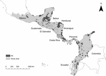
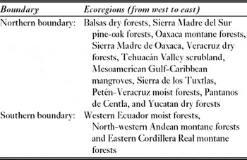
We used an established ecoregional classification (Olson et al. Reference Olson, Dinerstein, Wikramanayake, Burgess, Powell, Underwood, D'Amico, Itoua, Strand and Morrison2001) to define the study area, which included 53 WWF ecoregions in Mexico, Belize, Guatemala, Honduras, El Salvador, Nicaragua, Costa Rica, Panama, Colombia and Ecuador (Fig. 1). Marine habitats were excluded from the analyses, and the northern boundary was delimited by the Transvolcanic Belt of central Mexico. A transitional Nearctic-Neotropical biogeography region, including the area up to the Balsas depression, which has a greater influence of tropical Mesoamerican elements than central and northern Mexico, was also included (Morrone Reference Morrone2005). The southern boundary was delimited by the topographical transition where the Andes split into the three separate Cordillera ranges (Table 1).
Study region (light grey) delineated by the WWF ecoregions. The study area includes 10 countries from the Mesoamerica, Choco and tropical Andes regions. Current protected areas (PAs) according to the World Database on Protected Areas (2007) are indicated in dark grey.

Delimiting study area boundaries of ecoregions.

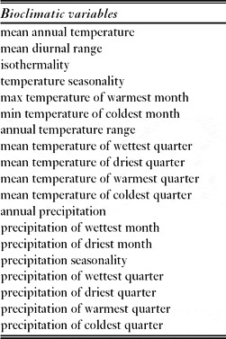
The environmental variables used included elevation, slope and aspect, with 19 bioclimatic variables (Table 2) from WorldClim (Hijmans et al. Reference Hijmans, Cameron, Parra, Jones and Jarvis2005). The WorldClim bioclimatic variables were developed using monthly temperature and rainfall values, which represent annual trends, seasonality and extreme or limiting environmental factors. We obtained the elevation above sea level from the US Geological Survey's Hydro-1K DEM data set (USGS [United States Geological Survey] 1998) and slope and aspect were derived by using the Spatial Analyst extension of ArcMap 9.0. All environmental layers were resampled at a 0.02° × 0.02° resolution in ArcGIS for a total of 437906 cells with an average area of 4.825 km2 (SD = 0.105; max = 4.946; min = 4.597).
The 19 bioclimate variables used as attributes in the environmental domain classification (from Hijmans et al. Reference Hijmans, Cameron, Parra, Jones and Jarvis2005).

We used the PATN v.3.11 software (Belbin Reference Belbin1989) to develop the environmental domain classifications. The input data was a matrix of 437906 rows and 22 columns, representing the values of each environmental variable (22 variables) within the study region (437906 cells). The ALOC algorithm (Belbin Reference Belbin1987), designed for large data sets, was used to construct a non-hierarchical classification that organized cells, based on an environmental distance measurement, into a number of predetermined groups or domains. All variables were equally weighted and the Gower metric distance measure was used to standardize the variables, which allowed for the combination of variables with different measurement units (Sneath & Sokal Reference Sneath and Sokal1973). This method of classification has been widely used (Leathwick et al. Reference Leathwick, Overton and Mc Leod2003; Trakhtenbrot & Kadmon Reference Trakhtenbrot and Kadmon2005; Mackey et al. Reference Mackey, Berry and Brown2008) to produce classifications unambiguously determined by specific variables, a process which makes the classification replicable and objective across the study area (Metzger et al. Reference Metzger, Bunce, Jongman, Mucher and Watkins2005).
Thirteen environmental domain classifications were constructed starting with 53 groups, which equals the 53 WWF ecoregions. The classification was increased by intervals of 50 groups until classification reached 653 groups; this was the maximum number of groups given the number of objects. To compare the correspondence between each of the 13 classifications and the WWF ecoregions, we used a tree diagram of similarity clusters for each classification, based on the relationship between the groups within each cluster. This was completed by calculating the average value for each environmental variable across the cells composing each group and thereafter organizing the groups within each classification using the Euclidian distance and unweighted pair-group average (UPGA) classification methods with the Statistica 8 software (StatSoft 2007). The UPGA clusters for each classification and the WWF ecoregions were compared by importing the classifications into ArcMap (ESRI [Environmental Systems Research Institute] 2004). In the tree diagram, the two groups most closely related were highlighted in ArcMap and then visually inspected to ensure that these groups were inside the geographical area of a specific WWF ecoregion. If the groups were within the area, we repeated the procedure, adding to the selection the next most similar group that conformed to the cluster. This process was repeated to determine if UPGA clusters were nested inside the WWF ecoregions.
The area occupied by each environmental domain in the WWF ecoregion was calculated for each classification using the projection ‘equal area cylindrical’ in ArcView extension Projector. This area was used as a multidimensional scaling in the Statistica 6 software to graphically observe if there was discrimination between ecoregions and if the degree of discrimination varied between classifications.
To evaluate the environmental diversity of the ecoregions and the environmental heterogeneity of representation in PAs, we selected those classifications that were nested within the WWF ecoregions and that could best discriminate between them. We calculated the Shannon diversity index as a measure of environmental or habitat diversity within each WWF ecoregion (sensu Pielou Reference Pielou1977) based on the area occupied by each environmental domain using the Species Diversity and Richness 3.02 software (Henderson & Seaby Reference Henderson and Seaby2002). For statistical comparisons of diversity, we used the upper and lower 95% confidence intervals for each Shannon diversity value. The area represented in the PA was calculated for each selected environmental domain classification (EDC) and for the WWF ecoregions by overlapping the datasets for the study region with the World Database on Protected Areas (WDPA 2007).
RESULTS
Classifications with ≥300 environmental domains were nested into WWF ecoregions. Conversely, classifications with <300 domains were not related to a particular WWF ecoregion. Clusters produced by classifications with ≥300 domains showed greater spatial correspondence with WWF ecoregions because the environmental domains were related to a specific geographical area. The results of visual comparisons were supported by multidimensional scaling, as ecoregions were discriminated by classifications containing ≥300 domains (Appendices 1 and 2, see supplementary material at Journals.cambridge.org/ENC). All multidimensional scaling analyses adequately fit to the Sheppard curve, indicating that two dimensions were sufficient to describe the data. From the 53 WWF ecoregions, 17 were discriminated by the multidimensional analysis.
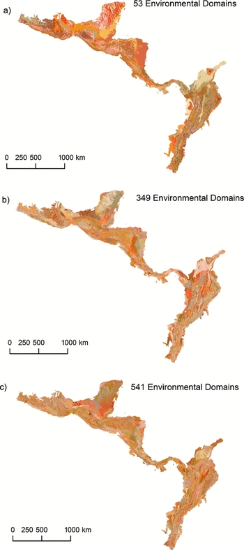
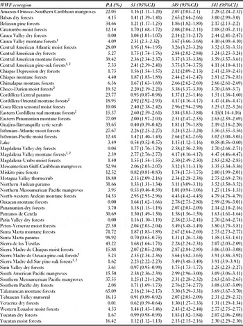
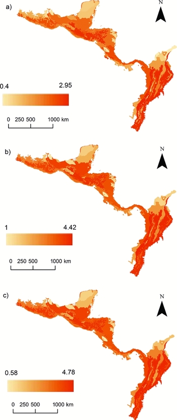
Given that there was no unique classification to improve discrimination between the WWF ecoregions, classifications of 349 and 541 environmental domains were selected for further analysis. The classification of 53 environmental domains was selected for a direct comparison with the 53 WWF ecoregions (Fig. 2Ia–c). These criteria provided a range of EDCs for evaluating our results. We found no significant differences in the environmental diversity between WWF ecoregions based on the three selected EDCs. The most environmentally-diverse ecoregions were the north-western Andean montane forest, the Magdalena Valley montane forest, the Eastern Cordillera real montane forest, the Cordillera Oriental montane forest and the Central American pine-oak forest. Conversely, ecoregions showing the least environmental diversity were Cordillera Central páramo, Lake, the Miskito pine forest, the northern Mesoamerica Pacific mangroves, the Santa Marta páramo and the Veracruz dry forest (Table 3). Overall, Shannon diversity values increased as the number of environmental domains increased with the exception of six ecoregions (Fig. 3, Table 3). Sierra de los Tuxtlas and Lake showed significantly greater Shannon diversity values (95% confidence intervals) for the 349 classification than for the 541 classification. Chimalapas montane forest, Cordillera Central páramo, Catatumbo moist forests and Veracruz dry forest showed no statistical difference in the Shannon diversity values (95% confidence intervals) between the 349 and 541 classifications (Table 3).
Environmental domain classifications (EDC) selected for further analyses. Each colour corresponds to a different domain in each classification. (a) 53 EDC, (b) 349 EDC and (c) 541 EDC.

Representation of the WWF ecoregions in protected areas (PAs) and the Shannon environmental diversity index (H) for the three selected environmental domain classifications (53; 349; 541). Values in brackets indicate lower and upper 95% confidence intervals of the Shannon index.1 Ecoregions with high environmental diversity and low representation in PAs.2 High conservation priority ecoregions.

Environmental diversity (Shannon index) for the WWF ecoregions based on the different classifications. (a) 53 EDC, (b) 349 EDC, and (c) 541 EDC. Colour scale indicates low environmental diversity with light colours and high environmental diversity with dark colours.

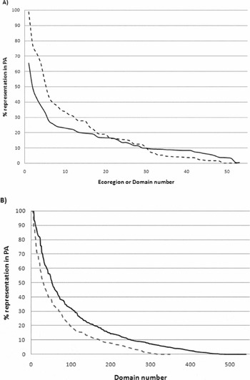
Few WWF ecoregions or environmental domains from the three EDCs were well represented in the PAs. This resulted in a logarithmic distribution when evaluating the representation of each ecoregion or environmental domain in the PAs (Fig. 4). The maximum percentage of PA area representation in the 53 EDCs was 65%. Conversely, the maximum percentage of PA area representation in the WWF ecoregions and in the 349 and 541 EDCs ranged between 98% and 100% (Fig. 4). Several ecoregions were consistently identified as having a low PA area representation, such as the Balsas depression, Sierra Madre del Sur and Chiapas mountains in Mexico, Central American mountain chains, Middle Magdalena, inter-Andean valleys, the Eastern Cordillera in Colombia and Western Moist Forest in Ecuador (Fig. 4; Appendix 3, see supplementary material at Journals.cambridge.org/ENC). The most environmentally-diverse WWF ecoregions were poorly represented in the PA (Table 3).
Percentage representation in PAs of (a) WWF ecoregions (dashed line) and 53 EDC (continuous line), and (b) 349 EDC (dashed line) and 541 EDC (continuous line). The logarithmic shapes of the curves indicate that few WWF ecoregions or environmental domains were highly represented in the PAs.

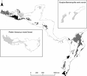
WWF ecoregions and environmental classification varied in PA representation. A high representation of an ecoregion in PA did not ensure appropriate representation of its environmental diversity. For example, 27.05% of Peten Veracruz moist forest was represented in the PA, which primarily covered the eastern sector of the ecoregion, leaving the western sector underrepresented. This selection highlighted the different environmental conditions in these areas according to the environmental classifications. Similarly, 35% of the Guajira Barranquilla Xeric-Scrub region area was inside the PA, and was concentrated on the Guajira peninsula, which disregarded the area around Barranquilla with different environmental domains (Fig. 5). Environmental domains showing less than 1% of their area inside the PA were identified as environmental domains with low representation in the PA and deserve high priorities for conservation. These regions represent unique environmental habitats and were outside all the PA (Fig. 5).
Environmental domains with less than 1% representation in the PAs, including the 53, 349 and 541 EDC, respectively. Environmental domains within high conservation priority ecoregions (compiled by Soutullo et al. Reference Soutullo, Castro and Urios2008) are depicted in black. Environmental domains within ecoregions with less than 10% representation in the PAs are depicted in dark grey. Environmental domains within ecoregions with more than 10% representation in the PAs are depicted in light grey. Insets illustrate examples of poorly representated environmental domains within two ecoregions with ≥10% representation in the PAs.

We identified three groups of environmental domains poorly represented in the PA, and where their inclusion improve environmental representation within WWF ecoregions: (1) environmental domains within high conservation priority ecoregions (Soutullo et al. Reference Soutullo, Castro and Urios2008), (2) environmental domains within ecoregions with less than 10% representation in the PAs, and (3) environmental domains within ecoregions with more than 10% representation in the PAs (Fig. 5). We set a value of 10% because the Convention on Biological Diversity (CBD 2002) stated that at least 10% of each of the world's ecological regions be effectively conserved.
DISCUSSION
WWF ecoregions have been used as a global template for assessments of species diversity, endemism or vulnerability, to identify conservation priority areas (Brooks et al. Reference Brooks, Mittermeier, Da Fonseca, Gerlach, Hoffmann, Lamoreux, Mittermeier, Pilgrim and Rodrigues2006). Local governments and international non-governmental organizations (NGOs) invest economic resources and conservation efforts in selected WWF ecoregions (Myers et al. Reference Myers, Mittermeier, Mittermeier, da Fonseca and Kent2000; Olson & Dinerstein Reference Olson and Dinerstein2002; Ferrier et al. Reference Ferrier, Powell, Richardson, Manion, Overton, Allnutt, Cameron, Mantle, Burgess, Faith, Lamoreux, Kier, Hijmans, Funk, Cassis, Fisher, Flemons, Lees, Lovett and Van Rompaey2004). Moreover, local governments usually use the WWF ecoregion classification to fulfil their obligations under CBD.
At a global scale, WWF ecoregion assessments provide a broad context for evaluating regional scale conservation priorities (Ferrier et al. Reference Ferrier, Powell, Richardson, Manion, Overton, Allnutt, Cameron, Mantle, Burgess, Faith, Lamoreux, Kier, Hijmans, Funk, Cassis, Fisher, Flemons, Lees, Lovett and Van Rompaey2004). We assessed climatic and topographic diversity at a regional scale across the WWF ecoregions from the Neotropical hotspots Mesoamerica, tropical Andes and Choco regions by selecting environmental domain classifications that maximized the overlap with WWF ecoregions. We observed that classifications of ≥300 environmental domains reflected the general pattern of the 53 WWF ecoregions, which highlighted the complexity of environmental conditions in the region. Our results showed that a maximum of 17 ecoregions could be clearly distinguished by a set of environmental domains, while 36 ecoregions could not be statistically discriminated. Other studies have shown similar results, indicating that WWF ecoregion classifications can only be partially described using environmental and biological data (Thompson et al. Reference Thompson, Shafer, Anderson, Strickland, Pelltier, Bartlein and Kerwin2004; McDonald et al. Reference McDonald, McKnight, Weiss, Selig, O'Connor, Violin and Moody2005). WWF ecoregions are defined as ‘relatively large units of land containing a distinct assemblage of natural communities and species with boundaries that approximate the original extent of natural communities prior to major land-use change (Olson et al. Reference Olson, Dinerstein, Wikramanayake, Burgess, Powell, Underwood, D'Amico, Itoua, Strand and Morrison2001). WWF ecoregions have been determined using a variety of ecoregion classification systems. As a result, the importance of each factor in determining characteristics of ecosystems can vary from region to region and with expert opinion because these characteristics have not been statistically defined (Metzger et al. Reference Metzger, Bunce, Jongman, Mucher and Watkins2005). Given the complexity of defining WWF ecoregions, it is difficult to predict correlations with environmental data (Thompson et al. Reference Thompson, Shafer, Anderson, Strickland, Pelltier, Bartlein and Kerwin2004). Environmental diversity is not a factor explicitly represented in the WWF ecoregion classification, which results in some ecoregions having more environmental diversity than others. Our study showed that similar patterns of diversity were maintained in the WWF ecoregions under different classifications; regardless of the number of domains included, some WWF ecoregions were consistently more diverse than others. Thus, using WWF ecoregions as an equivalent for conservation and management units can be misleading.
WWF ecoregion classification can also be inappropriate for assessing environmental representation. We do not intend to underestimate the relevance of WWF ecoregions worldwide, but rather caution about the possible shortcomings in application to conservation. WWF ecoregions provide robust biogeographic units reflecting the distribution of communities largely determined by historical processes, habitat type and large-scale ecological processes, which provide the critical spatial link between global priority setting efforts and site-based assessment (Wikramanayake et al. Reference Wikramanayake, Dinerstein, Loucks, Olson, Morrison, Lamoreux, McKnight and Hedao2002).
We found that the environmental diversity of a WWF ecoregion was not always appropriately represented in a PA, despite a >10% of PAs overlap with some WWF ecoregions, fulfilling the CBD conservation target. When large WWF ecoregions showed intermediate or high environmental diversity values, ecoregions’ representation in PAs did not necessarily reflect the environmental heterogeneity of an area (for example in the Peten-Veracruz moist forest and Guajira-Barranquilla xeric scrub ecoregions). Underestimation of environmental heterogeneity in the WWF ecoregions leads to inappropriate designation of PAs. Ferrier et al. (Reference Ferrier, Powell, Richardson, Manion, Overton, Allnutt, Cameron, Mantle, Burgess, Faith, Lamoreux, Kier, Hijmans, Funk, Cassis, Fisher, Flemons, Lees, Lovett and Van Rompaey2004) observed this is the result of the mismatch between the scale of global assessments and the scale at which conservation decisions occur. WWF ecoregions include extensive regions containing land of varying conservation value. There is a need to transition prioritization exercises from a global scale into actual conservation plans at the local level (Soutullo et al. Reference Soutullo, Castro and Urios2008). Conservation targets should be set to meet adequate representation of regional and local biodiversity.
Setting targets for adequate representation of biodiversity does not imply that total target values must increase with increasing diversity values; rather, this suggests that targets are established in an efficient way so that they achieve maximum representation of biological or environmental characteristics for the same target value (Margules & Sarkar Reference Margules and Sarkar2007). By effectively allocating the 10% target within WWF ecoregions, better representation of biological or environmental diversity is achieved. In this sense, the selection of conservation sites by a systematic conservation planning process is appropriate to maximize representation of biodiversity in PAs (Margules & Pressey Reference Margules and Pressey2000).
Low environmental heterogeneity representation can have adverse implications for conservation, particularly in Neotropical countries where detailed biological information is still lacking (Ferrier Reference Ferrier2002; Kim & Byrne Reference Kim and Byrne2006). Habitat heterogeneity is directly related to landscape diversity, suggesting that habitat selection and adaptation to local environmental conditions may be the primary processes structuring diversity among landscapes within the WWF ecoregions (Veech & Crist Reference Veech and Crist2007). If environmental domains are adequately represented in PAs, greater confidence in an adequate representation of habitat heterogeneity and regional species diversity is possible. Given the limited knowledge of detailed species distributions, a full range of environmental conditions should be present in PAs (Kirkpatrick & Brown Reference Kirkpatrick and Brown1994).
To effectively include different environmental conditions in PAs, selection should include classification of areas with similar ecosystem characteristics. Environmental domain classifications have been defined via a standardized method for simplifying environmental data into strata, which provides objective classification across a study region based on environmental variables. The development of a quantitative classification of environmental conditions is the first step towards producing tools to derive stratified samples (Bunce et al. Reference Bunce, Barr, Clarke, Howard and Lane1996; Metzger et al. Reference Metzger, Bunce, Jongman, Mucher and Watkins2005). This process is crucial when large-scale continuous gradients are involved and statistical analysis provides robust divisions based on the balance between the variables building the database (Metzger et al. Reference Metzger, Bunce, Jongman, Mucher and Watkins2005).
This is the first study to use the environmental domain classification at this scale to analyse the complex environmental diversity in the Mesoamerican, Chocó and tropical Andean regions (Myers et al. Reference Myers, Mittermeier, Mittermeier, da Fonseca and Kent2000). Other successful environmental classifications have been conducted for Papua New Guinea (Nix et al. Reference Nix, Faith, Hutchinson, Margules, West, Allison, Kesteven, Natera, Slater, Stein and Walker2000), Australia (Mackey et al. Reference Mackey, Berry and Brown2008), New Zealand (Leathwick et al. Reference Leathwick, Overton and Mc Leod2003), South Africa and Lesotho (Bonn & Gaston Reference Bonn and Gaston2005), in order to survey, monitor and manage biodiversity. Assessments of environmental classifications have shown that some environmental domains have received little conservation attention. Poor representation of environmental domains has been linked with areas of intensive human activity, which implies that there is a high economic cost when acquiring land for conservation. Moreover, governmental policies for actual reserve designation have focused on wild landscapes created by historical ad hoc decisions (Margules & Sarkar Reference Margules and Sarkar2007). The underrepresentation of some environmental domains will inevitably result in the differential loss of biodiversity features restricted to these environmental domains (Leathwick et al. Reference Leathwick, Overton and Mc Leod2003).
Environmental domain analysis cannot be used on its own to delineate reserves to encompass biodiversity. Species distributions are not always symmetrical in response to environmental gradients and do not have equal probabilities of distributions along the environmental space. Consequently, complementary areas may cluster around particular regions of high species density (Araújo et al. Reference Araújo, Densham and Humphries2003). Reserves selected on the basis of environmental domains are likely to represent more widespread biotic attributes in a satisfactory manner, but will probably fail to include many rare and endemic species and communities (Bonn & Gaston Reference Bonn and Gaston2005; Trakhtenbrot & Kadmon Reference Trakhtenbrot and Kadmon2006). Environmental domains poorly represent the location of species abundances, which will prevent the detection of potentially viable populations (Bonn & Gaston Reference Bonn and Gaston2005). Finally, environmental domain classifications indicate only the range of dynamic states expected at a site, but not the particular phase occurring at a particular site at a given time (Leathwick et al. Reference Leathwick, Overton and Mc Leod2003).
The effectiveness of environmental surrogates may be enhanced by using community-level modelling techniques in conjunction with the best available biological distribution data to define the relationship between environmental gradients and community richness and composition (Arponen et al. Reference Arponen, Moilanen and Ferrier2008). Several methods propose combined analyses, such as the environmental diversity approach (ED) (Faith & Walker Reference Faith and Walker1996; Faith Reference Faith2003; Faith et al. Reference Faith, Ferrier and Walker2004) and generalized dissimilarity modelling (GDM) (Ferrier et al. Reference Ferrier, Manion, Elith and Richardson2007). However, it is unclear how quality and quantity of biological data influence the environmental community modelling approach (Arponen et al. Reference Arponen, Moilanen and Ferrier2008).
Given that species distributions are influenced by climate variable correlations and their relationships with biotic attributes (Morin & Lechowicz Reference Morin and Lechowicz2008), research is needed to enable a better understanding of variable correlations with biological data. This will allow selection of subjective characteristics of environmental classifications, such as variables, weights given to the variables and number of groups, to produce classifications that better represent biological composition, ecosystem drivers and ecosystem responses reflective of ecological and evolutionary processes (Mackey et al. Reference Mackey, Berry and Brown2008).
Decisions for selecting modelling approaches depend on environmental, biological or community-level data availability, which will ensure that planning remains a dynamic process as better quality data become available. Incorporating other important environmental variables as they become available in better resolutions (such as soil type and topographical data), can better represent primary environmental regimens that drive biotic responses, such as heat, light, water and mineral nutrients. These advances may result in a classification that more accurately reflects the environmental domains, better representing species diversity (Mackey et al. Reference Mackey, Berry and Brown2008). If the limitations of using exclusively environmental information are considered, but the novelty of an objective comparison using environmental data across biological complex regions noted, regions where unique environmental conditions are underrepresented in the PAs may be identified. Our study suggests that conservation efforts should focus on poorly represented environmental domains in the PAs of relevant WWF ecoregions, such as the Chocó-Darién moist forest, the Cordillera Oriental montane forest, the Eastern Cordillera real montane forest, the Magdalena Valley montane forest, the Central American pine-oak forest and the Sierra Madre del Sur pine-oak forest (Soutullo et al. Reference Soutullo, Castro and Urios2008). Poorly represented environmental domains must be additionally included in conservation programmes in Mesoamerican, Chocó and tropical Andean countries where ecoregions contain environmental domains consistently underrepresented in the PAs. This includes the Balsas depression in Mexico, the Sierra Madre del Sur, the Chiapas Mountains ecoregions, the ecoregions across the mountain chains in Central America, the Middle Magdalena and the inter-Andean valleys ecoregions in Colombia, and the Western Moist Forest in Ecuador.
A preliminary assessment of conservation priorities using threatened species distributions in the same study region showed similar results for underrepresented biological data in PAs and identified similar regions for biological conservation, with the exception of the Middle Magdalena in Colombia (Sarkar et al. Reference Sarkar, Sánchez-Cordero, Londoño and Fuller2009). Geographic areas such as the Mesoamerican and Andean mountain chains and the inter-Andean valley, identified by biodiversity and environmental modelling approaches as being areas with conservation value, are often associated with high human population densities in urban settlements; this creates many challenges to accurately determining conservation areas and requires integrative landscape management and innovative restoration perspectives to ensure biodiversity conservation (Ervin Reference Ervin2003; Rodrigues et al. Reference Rodrigues, Andelman, Bakarr, Boitani, Brooks, Cowling, Fishpool, da Fonseca, Gaston and Hoffmann2004; Fuller et al. Reference Fuller, Munguía, Mayfield, Sánchez-Cordero and Sarkar2006; Margules & Sarkar Reference Margules and Sarkar2007; Chan & Daily Reference Chan and Daily2008; Sarkar et al. Reference Sarkar, Sánchez-Cordero, Londoño and Fuller2009).
ACKNOWLEDGEMENTS
We wish to thank N. Bayly, N. Urbina and S. Sarkar for constructive comments. M. Londoño-Murcia was supported by a doctoral scholarship from Consejo Nacional de Ciencia y Tecnología (CONACyT) and Posgrado en Ciencias Biológicas, Universidad Nacional Autónoma de México. Víctor Sánchez-Cordero was supported by the Consejo Nacional de Ciencia Tecnología (Project 25048).