1 Introduction
The study of the fluid motion above and through natural and engineered surfaces is a challenging task, particularly if the surface possesses small-scale features which exert (or are believed to exert) an important fluid-dynamics-related role, whose effect cannot be captured directly by a numerical simulation because of the difficulty in addressing all the fine-grained details of the fluid/wall coupling. Such details might include the effect of the surface texture, its porosity, compliance and the interactions between the flow of the outer fluid and that of a different fluid which may be trapped within near-wall microcavities. It then becomes useful to employ an approach capable of replicating the important features near the wall at a fraction of the computational cost of a full, detail-resolving simulation – one such approach is multiscale homogenization.
Before employing any modelling approach in the effort to replicate a specific function of a natural organism, we must, however, realize that biological evolution has gone over millions of years with its own laws and constraints, in a way not limited by the current biases of human thought. This implies that mere imitation of nature does not yield an optimal solution for a specific purpose; evolution has progressed in a multi-objective fashion, relying on the introduction of novel traits to provide natural selection something to act upon. Thus, many primary functions in the natural world, such as finding a partner or escaping a predator, do not translate into relevant objectives for an engineering device. Bio-inspiration, not bio-imitation, is the keyword. In this Perspective article, we limit ourselves to mechanical effects produced at the interface between a natural surface and a fluid, such as air or water, with the exclusion of chemical, molecular or atomic interactions. Despite the fact that we are speaking throughout this article of small-scale features and effects, we will always remain in the realm of continuum mechanics, to analyse the interactions of fluids with the heterogeneous, anisotropic, rough, porous and/or compliant substrates which can be found in biological settings. Beyond their interest per se, understanding how natural surfaces operate, joined with the ability to model their coupling to the fluid which surrounds them, will provide insight into the design of passive and active flow actuation systems for technological applications, for example, to reduce drag or mitigate noise, and guide the development of innovative microsensors.
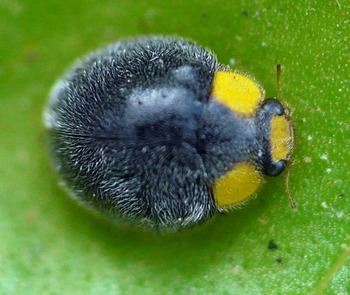
A 3 mm long yellow shouldered ladybird (Apolinus lividigaster), common in Australia and New Zealand. Picture courtesy of Robert Whyte.

Before proceeding to describe the theory used to model microstructured media and interfaces, we take a brief detour to illustrate some of the rich varieties of functions and shapes of natural and engineered surfaces.
1.1 From biological to engineered surfaces
Examples of inspiring natural surfaces abound, although their fluid-mechanics-related functions and characteristics, if any, usually only unfold under the microscope. In the animal kingdom we start by making reference to the many species of insects whose wings are covered by setae/bristles, such as the membranous wings of the terrestrial adults of the order Trichoptera (thrix in Greek means hair) or of the order Coleoptera (see, for example, the picture of the Coccinellidae in figure 1). The dense hairy coat on the wings of this lady beetle (the mean spacing between adjacent hairs is of order
 $20~\unicode[STIX]{x03BC}\text{m}$
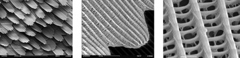
) suggests a water repelling effect. Another example comes from the order Lepidoptera, which includes moths and butterflies, and whose wings are covered with thousands of scales. Such scales (shown, at different magnifications, in the three frames of figure 2) are porous, and air can flow through tiny pores below the outer lamina, reaching the inner, impermeable surface. The outer lamina consists of ridges, of periodicity equal to a few microns and connected by tiny cross-bars; it is maintained separated from the inner lamina by post-like structures, called trabeculae. Such a complex microstructure has a role in light absorption and refraction, but is also very efficient in reducing the wettability of the wings, thus allowing their self-cleaning under rain or dew (Perez Goodwyn et al.
Reference Perez Goodwyn, Maezono, Hosoda and Fujisaki2009). Another possible role of the hollow region below the grooves of butterfly scales has been discussed by Kovalev (Reference Kovalev2008), who conducted wind tunnel experiments on a flapping model of the scale of the butterfly Pyrameis atalanta, arguing for an increase in lift of approximately
 $15\,\%$
when compared to a similar model in the absence of pores.
Electron microscopic images of the scales of the European peacock butterfly (Aglais io). Images by SecretDisc, Creative Commons BY-SA 3.0.

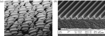
Electron microscopic images of (a) the dermal denticles of a lemon shark (Negaprion brevirostris) and (b) trapezoidal riblets. Left image by Pascal Deynat/Odontobase, Creative Commons BY-SA 3.0. Right image courtesy of Fraunhofer IFAM.

The scales over the wings of moths and butterflies are not too dissimilar (including the size, with a characteristic length of the order of
 $100~\unicode[STIX]{x03BC}\text{m}$
in both cases) from the dermal tooth-like denticles which cover the body of sharks. Such denticles, pictured in figure 3(a), display typically three to five ridges whose spacing is close to the riblet spacing for optimal skin friction drag reduction (Bechert & Bartenwerfer Reference Bechert and Bartenwerfer1989). The mechanism by which riblets (figure 3
b) work, despite the increase in wetted area, stems from the large skin friction decrease in the valleys of the riblets compared to a smooth surface under the same flow conditions, which more than compensates the mild increment towards the riblets tips (Hooshmand, Youngs, Wallace & Balint Reference Hooshmand, Youngs, Wallace and Balint1983).
As opposed to prototypical riblets, the shark skin above which denticles are placed is elastic, and sharks can bend and flex their body while swimming. The long-scale undulations of the flexible dermis of sharks dramatically reflect onto their propulsion characteristics, as shown experimentally by Oeffner & Lauder (Reference Oeffner and Lauder2012) through the use of a real shark skin attached to a flexible membrane-like foil, set into motion by a robotic flapping device that mimics the movement of real sharks. The reason for the increase in thrust force measured by Oeffner & Lauder (Reference Oeffner and Lauder2012), compared to the rigid plate case and to the flexible case with the denticles sanded off the dermis, appears to be related to the presence of an intense leading edge vortex adhering closely to the foil surface. Such a vortex generates a suction force with a component along the free-stream direction (thus propulsion is enhanced) whereas in the rigid or sanded cases the vortex is weaker and positioned farther away from the leading edge of the foil. This explanation has been later corroborated by Wen, Weaver & Lauder (Reference Wen, Weaver and Lauder2014). The latter authors used a three-dimensional printing technique to fabricate rigid denticles and anchored them onto a flexible membrane substrate, comparing results to the case of a smooth membrane under identical flow conditions. When both the synthetic shark skin and the smooth membrane were held still in the water channel, the synthetic skin experienced a lower drag by up to
 $9\,\%$
; this reduction turned into a drag increase when the periodicity of the denticles exceeded a value of approximately
 $13$
(expressed in wall units), a behaviour consistent with that of riblets. When the foils were made to heave and pitch, conditions were found for which the printed shark skin required less energy to swim over a given distance and was more efficient than the smooth foil, as a result of increased thrust generation. There is thus evidence that the hydrodynamical performance of sharks results from both the complex three-dimensional, small-scale structure of the denticles and the long-scale deformation of the skin, related to its flexibility. Consequently, any realistic modelling effort should considered the coupled fluid–solid problem.
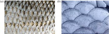
The scales of other fish families display a variety of shapes and sizes; cycloid and ctenoid scales are found on the majority of living bony fish, the main difference being that ctenoid scales feature several small comb-like spines (cf. figure 4). Scales growing on the dermis of fish are covered by a fine outer skin layer (epidermis) containing mucus-secreting glands. Mucus gives fish their slippery feeling associated with excellent drag-reducing properties, as demonstrated experimentally by Rosen & Cornford (Reference Rosen and Cornford1971) who used a flow rheometer to test a variety of fish mucuses in a water solution at varying dilutions. It seems that mucus from fast, predatory fish (such as the Pacific barracuda) is generally most effective, with frictional drag which decreases by
 $65\,\%$
when a
 $5\,\%$
mucus–seawater mixture is tested. The reason for the substantial drag reduction in turbulent flow conditions goes by the name of the ‘Toms effect’ in the fluid mechanics community and has been known for a long time (Toms Reference Toms1948). The inclusion of additives, e.g. a small percentage of high molecular weight polymers in water, micellar surfactant systems, bubbles, rigid fibres or even solid spheres, can lead to drag reduction, and this has important potential implications for the reduction of energy losses in pipelines, in marine and underwater vehicles. For the case of polymers, the physical argument is that polymer chains are stretched by the mean shear in the near-wall region, causing a stretching of the near-wall streaks and a consequent mitigation of the intensity of the quasi-streamwise vortex structures in the buffer layer. These vortices drive momentum transport to/from the wall, and their weakening results in drag reduction. Beyond its hydrodynamic function, fish mucus plays a role also in the fish reproductive behaviour, in respiratory gas exchange, in ion and water regulation, in disease resistance, etc. (Shephard Reference Shephard1994).
(a) Cycloid scales of a common roach (Rutilus rutilus). Image by kallema, Creative Commons BY-SA 3.0. (b) Ctenoid scales of a paradise fish (Macropodus opercularis). Picture by Sue Lindsay © Australian Museum. The characteristic dimension of cycloid scales on the left is 1 cm, approximately ten times more than that of ctenoid scales, on the right.

Whereas fish (and reptiles) have scales on their dermis, other vertebrates have hair (mammals), believed to act mainly as sensory organs and/or to provide insulation against heat loss, and others yet have feathers (birds).
A marine mammal who has undergone some fluid dynamics scrutiny recently is the fur seal, a pinniped of the Arctocephalinae subfamily, covered with a dense layer of hair. Itoh et al. (Reference Itoh, Tamano, Iguchi, Yokota, Akino, Hino and Kubo2006) glued a real fur sample onto a test surface, and rendered it hydrophilic by a tannin treatment, before testing it comparatively against a smooth surface and a surface with riblets in a channel of rectangular cross-section filled with either water or with a glycerol–water solution. The seal’s hair was oriented along the streamwise direction and displayed a range of spanwise wavelengths from 2 to 18 (when measured in wall units, for a Reynolds number, based on bulk speed and hydraulic diameter of the channel, equal to 7000), against a single wavelength of 7 wall units for the case of trapezoidal riblets tested under the same conditions. The notable result by Itoh et al. (Reference Itoh, Tamano, Iguchi, Yokota, Akino, Hino and Kubo2006) was that drag was consistently reduced by more than 10 % over a wide range of Reynolds numbers (whereas the maximum skin friction reduction was 7 % for the surface with riblets), and this was associated with a weaker streamwise turbulence intensity. Among the factors which could possibly have produced such a result, the effect of the flexibility of the hair was mentioned by Itoh et al. (Reference Itoh, Tamano, Iguchi, Yokota, Akino, Hino and Kubo2006), related to the ability of the elements of the hairy coating to re-orient with, and adapt to, the flow.
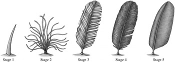
The currently accepted model of evolution of feathers (Prum Reference Prum1999). Stage 1: unbranched quill. Stage 2: simple filaments attached to a central point. Stage 3: main shaft (rachis) with primary branches (barbs). Stage 4: rachis with rows of barbs and interlocking secondary branches (barbules); the interlocking takes place via small hooks called barbicels. Stage 5: fully developed, asymmetrical flight feather. Image courtesy of Emily A. Willoughby.

The plumage of birds makes for an interesting story. Until recently, common belief was that feathers had evolved from reptilian scales for the purpose of conferring flying properties to proto-birds (cf. the entry on the Encyclopaedia Britannica at the time of writing). Prum (Reference Prum1999) developmental theory, now largely accepted, focused instead on how feathers grew and acquired structural complexity, without specific reference to the aerodynamic context. The finding of fossils of small, non-flying, feathery, theropod dinosaurs in China, displaying the different feather stages predicted by Prum’s theory, provides, to date, the strongest support to the theory. The proto-feathers and feathers described by Prum (Reference Prum1999) and displayed in figure 5 can still be found in different parts of the wings and body of modern birds. Each feather’s type is associated with certain functions. The most notable are feathers in the wings and tail of birds, which play mostly an aerodynamic and flight control role, and plume-like feathers used mainly for insulation purposes. The structure of feathers also provides for water repellence, as probably first observed by Cassie & Baxter (Reference Cassie and Baxter1944) who argued that ‘man’s attempts to make clothing with the water-repellency of a duck should be directed to perfecting an appropriate cloth structure rather than, as at present, to searching for an improved water-repellent agent’. Today it is thought that it is the two-scale structure of the feather vane which renders it exceptionally waterproof, with air trapped underneath the network of barbs and barbules (Bormashenko et al. Reference Bormashenko, Bormashenko, Stein, Whyman and Bormashenko2007).
Probably the best example of engineering device, directly inspired by the long flight feathers at the tip of birds’ wings and which has now become commonplace in aircraft, is represented by the winglet, a wingtip protuberance which aims at reducing lift-induced drag. Over the past thirty years many bio-inspired winglet shapes have been proposed, including variable cant angle winglets, blended winglets and spiroid wing tips. Other feathers, called coverts, are present on the suction side of wings and hold (also) a dynamic role: they pop up and vibrate when the bird encounters gusty winds or flies at large angles of incidence (for example during a perching manoeuvre). Such an occurrence alleviates the stall behaviour of the wings, maintaining adequate lift, since the raised feathers prevent the region of reversed flow to spread from the trailing edge all the way to the leading edge of the wing, as shown in model experiments by Bechert et al. (Reference Bechert, Bruse, Hage and Meyer2000). Flight tests on a STEMME S10 motor glider, equipped with self-activated, movable flaps, demonstrated that stall was delayed as the angle of attack was gradually increased, when compared to the configuration without movable flaps (Bechert, Hage & Meyer Reference Bechert, Hage, Meyer and Liebe2007). Such positive results, obtained with high aspect ratio wings and a basically two-dimensional flow, were not confirmed when swept and tapered wings were tested in the wind tunnel, highlighting the difficulty in adapting a simple, working solution to a different configuration.
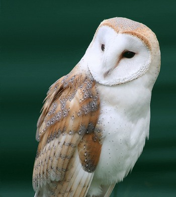
Barn owl (Tyto alba). Photo by Steve Brace, CC BY 2.0.

Another important role which feathers can play is related to noise (or lack thereof). Some species of predatory birds (the owl in particular, shown in figure 6) do not fly very fast, but are so silent as to not be perceived by their prey. The most extensive recent scrutiny of the flight apparatus of the barn owl has been conducted by Bachmann (Reference Bachmann2010), as a basis for studying silent flight. He described (i) the serrations at the leading edge of some of the primary flight feathers, acting as turbulence generators and leading to a stable air flow along the distal wing, (ii) the velvet-like texture on the dorsal surface of all feathers, with the porosity of this structure capable to effectively reduce friction noise and (iii) the flexible fringes at the trailing edge of the feathers, formed by barb endings, able to limit the broadband scattering noise in the wake. These three aspects have been scrutinized independently in a large number of theoretical, numerical and experimental studies, mostly using static wing models. For example, experiments by Hersh, Soderman & Hayden (Reference Hersh, Soderman and Hayden1974) demonstrated the ability of wings with leading edge serrations to mitigate aerodynamic noise; trailing edge noise has been theoretically investigated by Jaworski & Peake (Reference Jaworski and Peake2013), who argued that the porous, compliant nature of the outer fringes can reduce the edge scattering mechanism; the velvet-like covering on the suction side of wings was tested by Clark et al. (Reference Clark, Daly, Devenport, Alexander, Peake, Jaworski and Glegg2016), who found a reduction in the pressure fluctuations on the surface, as a function of the surface density of the downy fibres. Probably it is a combination of all of these effects, coupled to a slow wing beat, which confers acoustic stealth to owl flight.
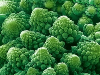
Also the plant kingdom provides for many interesting examples of surfaces/substrates capable of inspiring new functionalized surfaces and flow control techniques. One of the best known examples is the leaf of the plant Nelumbo nucifera (known as sacred lotus) which exhibits remarkable superhydrophobicity. Several other plants have a similar property, such as the Salvinia oblongifolia or the Brassica oleracea (Koch & Barthlott Reference Koch and Barthlott2009) (cf. figure 7). A drop of water placed onto a superhydrophobic substrate maintains a quasi-spherical shape, does not wet the surface and slides easily away. These properties arise from a combination of surface texture and interfacial energy. On the one hand, a low surface energy material guarantees low wettability of the surface; on the other, nano- or micro-roughness elements permit the maintenance of a stable air layer, minimizing the contact between the liquid and the solid. On submerged leaves the presence of a gas film contributes to the survival of the plant, enhancing the exchange of
 $\text{O}_{2}$
and
 $\text{CO}_{2}$
with the water, allowing for underwater photosynthesis and respiration; furthermore, the self-cleaning property of superhydrophobic surfaces and the limited availability of water are believed to provide defence against pathogens, such as fungi and bacteria (Koch & Barthlott Reference Koch and Barthlott2009).
Magnified image of the flower head of a green cauliflower (Brassica oleracea). Photo credits: Brandon Broll.

At the other end of the spectrum stand superhydrophilic leaves, with high affinity to water. They either absorb water through their surface pores to remain permanently wet, or they let water spread easily across their surface. The most striking example is the Ruellia devosiana which is also superoleophilic (Koch et al. Reference Koch, Blecher, König, Kehraus and Barthlott2009). The leaf surface has a high interfacial energy; this aspect, combined with the channel-like structures formed by the leaves’ superficial cells, translates into fast water-spreading properties. This characteristic is believed to protect the plant against the formation and proliferation of micro-organisms, called biofilm.
The self-cleaning ability of both superhydrophobic and superhydrophilic coatings can be exploited, in different manners, against the formation of biofouling on naval vessels and infrastructures, a major economic burden for the maritime industry. Reviews of such abilities are provided by Kirschner & Brennan (Reference Kirschner and Brennan2012) and Liu & Jiang (Reference Liu and Jiang2012). Another class of materials which presents anti-fouling properties is that of lubricant-infused materials. These are microstructured, porous materials with a layer of lubricant liquid, immiscible and unreactive with water, interposed between the solid surface and water. After reviewing the ability of lubricant-infused surfaces to repel organic, aqueous and complex liquids, and to fight fouling by bacteria, blood and algae, Amini et al. (Reference Amini, Kolle, Petrone, Ahanotu, Sunny, Sutanto, Hoon, Cohen, Weaver and Aizenberg2017) demonstrated, under both controlled laboratory conditions and in marine field tests, that the lubricant film was also very effective against adhesion by mussels, among the most ubiquitous marine macrofoulers.
By changing the scale of view, we can look at a whole plant; the interactions between the flow of water or air and plants play an important role in mediating hydrological, geomorphological and biological processes. Plants are often slender and flexible and are susceptible to being deformed by the flow, this effect is called reconfiguration and results in reduced resistive forces (Alben, Shelley & Zhang Reference Alben, Shelley and Zhang2002; Gosselin, de Langre & Machado-Almeida Reference Gosselin, de Langre and Machado-Almeida2010). If multiple plants are involved, we can have collective effect such as the waving of a crop field under the effect of wind, or of a seagrass bed deformed by the motion of water. The organized behaviour of systems of plants goes by two Japanese words: honami (when in air) and monami (in water), and a rich literature exists on these phenomena (de Langre Reference de Langre2008; Nepf Reference Nepf2012). The interaction between the plants and the flow occurs particularly near the top of the vegetation; the mean flow has a distribution similar to that of a mixing layer and a system of large-scale vortices of the Kelvin–Helmholtz type appears near the interface (Ghisalberti & Nepf Reference Ghisalberti and Nepf2002). The interest in this type of interaction stems from the possibility of replicating them at different spatial and temporal scales by engineering devices to, for example, sense the wall shear stress (cf. the flexible micropillars designed by Brücker, Spatz & Schröder (Reference Brücker, Spatz and Schröder2005)) or actively control the surface skin friction (this is the case, for example, for the microscopic flap actuators described by Ho & Tai (Reference Ho and Tai1998)). Another passive control technique has been employed by Hasegawa & Sakaue (Reference Hasegawa and Sakaue2018); they used an electrostatic flocking technique to cover portions of the external surface of a cylinder with nylon polyamide fibres. The cylinder was then placed in a wind tunnel run at a velocity of
 $20~\text{m}~\text{s}^{-1}$
(the Reynolds number, based on the diameter,
 $D=50$
mm, of the cylinder was equal to
 $6.1\times 10^{4}$
) and the effect of the various coatings assessed. When thin and short fibres were employed, a drag reduction of up to 50 % was achieved when a short (along the azimuthal direction) coating was placed in the most sensitive region, i.e. somewhere upstream of the flow detachment point of the smooth cylinder configuration. This reduction in pressure drag was accompanied by a narrowing of the wake region. Longer fibres displayed some drag-reducing capabilities when placed in the aft of the cylinder, in the separated region. Similar effects had been reported previously in laminar flow conditions (Favier et al.
Reference Favier, Dauptain, Basso and Bottaro2009).
We have exposed a brief overview of exemplar coatings from nature and of a few engineering systems which might have been inspired by them; clearly, the biological surfaces which can possibly be modelled are limitless, as are the functions they carry out. Bio-mimicry can guide in the functionalization of materials via a combination of physical (texturing/patterning) and chemical modifications (for example by the addition of surfactants or lubricants, or varying the surface energy of the material). The dynamic coupling between the material and the fluid should also be examined attentively; biological systems are immersed in a fluid and interact with it in many ways. Putting these pieces together represents a challenge for generations of scientists to come.
1.2 What are we interested in and how can homogenization help?
This paper describes a technique to treat media and interfaces similar to those described above, by replacing the fine-scale structure with appropriately averaged properties. The need to use some averaging, or upscaling, procedure stems from the fact that the length scale of the macrostructure (
 $L$
in the following) is typically much larger than the length scale (
 $l$
) of heterogeneities. Accordingly, a numerical resolution of the full problem might result in a mesh resolution beyond the storage or processing capabilities of modern computers, if one were not to smooth microscale details via some averaging process. The continuum concept in engineering mechanics is a prime example of homogenization, and properties such as the elastic modulus of a solid or the viscosity of a fluid are homogenized quantities.
The word homogenization was probably coined by Babuška (Reference Babuška and Hubbard1976) who described it as ‘the approach which studies the macrobehaviour of a medium by its microproperties’, by replacing the rapidly varying properties of a ‘heterogenous material’ with those of ‘an equivalent homogeneous one’. A heterogeneous material is one which is composed of domains made by different materials or phases, such as a composite or a porous matrix. The ‘equivalent’ properties which arise from the solution of auxiliary problems defined in ‘microscopic domains’ go by the name of macroscopic, apparent or effective properties. It should already have been clear that the prefix micro used throughout this paper does not refer to the actual size of
 $1~\unicode[STIX]{x03BC}\text{m}$
, but to the length scale difference between the internal scale of the medium or interface and a relevant macroscopic one.
Homogenization theory applies to a variety of fields in physics and properties of interest range from the thermal conductivity of a heterogeneous medium to the stiffness tensor of an elastic multi-layered material, from the permeability of a porous matrix to the magnetic conductivity of some electrically conducting media. The majority of applications of the theory have so far dealt with problems in solid mechanics, and techniques to homogenize material properties, including approaches to statistically characterize the microstructure when local properties have a random distribution, are described in a large number of monographs and books (see, e.g. Torquato Reference Torquato2002). A contribution dedicated to problems related to the percolation of fluids through porous media, which attempts to bridge the gap among various approaches and approximations, has been edited by Hornung (Reference Hornung1997).
The technique discussed in the present paper is limited to the simple case in which the microstructure of the media or interfaces is periodic; the existence of two well-separated length scales renders the governing differential equations amenable to a solution via a formal asymptotic expansion in terms of a small parameter
 $\unicode[STIX]{x1D716}=l/L$
, so that results can in principle be searched up to any order of accuracy in
 $\unicode[STIX]{x1D716}$
. The particular adjoint approach described here extends straightforwardly to nonlinear equations in which case it results in a strong coupling between micro- and macroscale fields. The ensuing non-locality of the effective parameters of the macroscale equations is a known challenge. While the literature reports mostly mathematical, rather than practical, results (see, e.g. Lions et al.
Reference Lions, Lukkassen, Persson and Wall2001), it is aimed for the approach presented herein to also guide in the development of practical models for the homogenization of nonlinear problems.
Before proceeding further, it is useful to say something on the notations used throughout the paper: a hat over a variable name denotes a dimensional variable, the corresponding dimensionless quantity being indicated without the hat. The dimensional velocity components are noted as
 $\hat{U} :=\hat{U} _{1}$
,
 $\hat{V}:=\hat{U} _{2}$
and
 ${\hat{W}}:=\hat{U} _{3}$
, along the streamwise (
 $\hat{X}:=\hat{X}_{1}$
), wall/interface-normal (
 ${\hat{Y}}:=\hat{X}_{2}$
) and spanwise (
 $\hat{Z}:=\hat{X}_{3}$
) directions. Subscripts and names of dimensionless variables follow the same convention. Finally, non-dimensional variables indicated with capital letters are generally of macroscopic type, while small letters are normally reserved for microscopic quantities.
2 A step back in time: to slip or not to slip?
Until the early nineteen century engineers were mostly concerned with empirical formulas, and mathematicians (‘geometers’) with theories of unresisted flows. However, the problem of the possible slippage of a viscous fluid above a solid surface and the resistance opposed by a wall to a fluid in motion near it were present long before the day the equations ruling the motion of viscous fluids were first derived. For example, Jean le Rond D’Alembert explained the paradox which now bears his name by the ‘tenacity and adherence of the fluid particles’ responsible for the fore–aft asymmetry of the fluid motion, even for rear–front symmetric bodies. Henri Navier seemed to have been convinced of the fact that fluid particles adhere to solid walls, before settling for a slip condition (Navier Reference Navier1823) in the effort to match experimental results by Pierre-Simon Girard for the flow in capillary tubes (a detailed historical account of the early days of hydrodynamics can be found in the book by Darrigol (Reference Darrigol2005)). In his seminal paper, Navier derived the equations governing the motion of a viscous, incompressible fluid starting from first principles, by considering interactions between ‘molecules’. He also stated that the ‘molecules in the proximity of solid walls can only move in the plane of the walls’, with the solid surface exerting a resistance to the motion proportional to the slip velocity,
 $\hat{U} _{s}$
.
By equating the shear stress exerted by the fluid onto the wall,
 $\unicode[STIX]{x1D707}\,\text{d}\hat{U} /\text{d}{\hat{Y}}$
, to the resistance opposed by the wall, assumed proportional to the slip velocity, Navier concluded that at a fixed wall the boundary condition read
 $$\begin{eqnarray}\hat{U} _{s}=\hat{\unicode[STIX]{x1D706}}\frac{\text{d}\hat{U} }{\text{d}{\hat{Y}}},\end{eqnarray}$$
and likewise for the spanwise component of the velocity. The constant of proportionality
 $\hat{\unicode[STIX]{x1D706}}$
, today called Navier’s slip coefficient or slip length, is a function of the dynamic viscosity,
 $\unicode[STIX]{x1D707}$
, of the fluid and of the ‘nature of the bodies with which the fluid is in contact’.
Navier’s contemporaries do not seem to have paid much attention to his fundamental theoretical contribution and the equations ruling the flow of viscous fluids, both in the incompressible and in the compressible forms, were rederived independently a few other times and eventually put in the modern form used today by Stokes (Reference Stokes1845). The boundary condition for the fluid next to a solid wall remained, however, a matter of controversy; Stokes himself started using a slip condition before deciding for no slip a few years later.
The problem was eventually settled – and the empirical no-slip condition universally accepted – when Taylor (Reference Taylor1923) demonstrated that, using no slip at the walls, perfect agreement could be achieved between theory and experiments near the onset of the first instability for the flow between differentially rotating cylinders.
In actuality, no slip still poses problems in some situations where small-scale effects at the wall and molecular interactions among different fluids and a solid surface occur. A well-known example is that of a liquid (a small drop or a rivulet) spreading down an incline. The use of the no-slip condition at the leading edge triple line yields an infinite force singularity which needs to be removed for the continuum equations to be tenable (Dussan Reference Dussan1979). The numerical remedy usually adopted consists in either using a thin precursor film or in enforcing a slip condition. There is no clear criterion, however, on the choice of either the thickness of the precursor film or the slip length. Another case, discussed further in the following, for which a slip condition applies is that of the flow over rough, superhydrophobic or lubricant-impregnated surfaces.
Incidentally, it is of interest to note that the same condition (2.1) given by Navier was derived also by Maxwell (Reference Maxwell1879) on the basis of a scattering model for the case of a rarefied gas in the absence of heat flux between the gas and the wall, when
 $0.01\lesssim Kn\lesssim 0.1$
, where the Knudsen number,
 $Kn$
, is the ratio of the mean free path of the gas molecules to the characteristic length of the system.
3 Difficulties with one of the simplest cases of dividing surfaces: Poiseuille flow over a porous bed
Probably the simplest case of a dividing surface is that which separates a region of incompressible laminar flow in a plane channel (the so-called free-fluid domain) from a second region formed by alternating, fixed solid grains and pores, with fluid which saturates the pores and slowly moves through them. If the driving pressure gradient is sufficiently small we can assume that the free-fluid region is ruled by Stokes’ equation whereas the motion in the porous medium can be described by Darcy equation. This dividing surface is thus also called the Stokes–Darcy interface.
The situation we consider is represented in figure 8. The macroscopic free-fluid domain extends from
 ${\hat{Y}}=0$
to
 ${\hat{Y}}=2L$
and the porous region occupies the space
 ${\hat{Y}}\leqslant 0$
. The pressure gradient acts along
 $\hat{X}$
, in both the channel and the porous layer, so that only a streamwise velocity component is non-zero. The porous medium is assumed isotropic and its permeability is a scalar quantity, denoted by
 $\hat{{\mathcal{K}}}$
.
Sketch of the configuration by Beavers & Joseph (Reference Beavers and Joseph1967).

Beavers & Joseph (Reference Beavers and Joseph1967) observed that the flow rate in the channel was larger in the presence of the porous layer than with a no-slip wall at
 ${\hat{Y}}=0$
and hypothesized that the fluid could slip with a velocity
 $\hat{U} _{s}$
at the Stokes–Darcy interface. Their dimensional semi-empirical condition reads
 $$\begin{eqnarray}\hat{U} _{s}=\langle \hat{u} ^{(0)}\rangle +\frac{\hat{{\mathcal{K}}}^{1/2}}{\unicode[STIX]{x1D6FC}_{BJ}}\frac{\unicode[STIX]{x2202}\hat{U} }{\unicode[STIX]{x2202}{\hat{Y}}}\biggm\vert_{{\hat{Y}}\rightarrow 0^{+}},\end{eqnarray}$$
with
 $\langle \hat{u} ^{(0)}\rangle$
the seepage velocity through the porous medium, evaluated some distance below the dividing surface; the angle brackets in (3.1) denote volume averaging (see later definition (4.11)) and
 $\unicode[STIX]{x1D6FC}_{BJ}$
is a dimensionless parameter of order one, which is a function of the properties and the geometry of the permeable material near the dividing surface, of the local direction of the flow, of the Reynolds number and of the possible presence of structural non-uniformities at the surface of the porous medium (Larson & Higdon Reference Larson and Higdon1986; Sahraoui & Kaviany Reference Sahraoui and Kaviany1992). Structural non-uniformities are hardly avoidable in practice since, near the interface, solid inclusions cannot pack as tightly as elsewhere in the porous layer and the porosity is locally larger.
The Darcy velocity is
 $\langle \hat{u} ^{(0)}\rangle =-(\hat{{\mathcal{K}}}/\unicode[STIX]{x1D707})(\text{d}\hat{p}^{(0)}/\text{d}\hat{X})$
(cf. § 4) with
 $\text{d}\hat{p}^{(0)}/\text{d}\hat{X}$
the macroscopic pressure gradient and
 $\hat{{\mathcal{K}}}$
an order-
 $l^{2}$
quantity (so that the dimensionless permeability is
 ${\mathcal{K}}=\hat{{\mathcal{K}}}/l^{2}$
), where
 $l$
represents a characteristic dimension of the pores (or of the solid inclusions). As anticipated,
 $\unicode[STIX]{x1D716}=l/L$
is a small parameter.
Eventually, the slip velocity reads (Beavers & Joseph Reference Beavers and Joseph1967)
 $$\begin{eqnarray}\hat{U} _{s}=\unicode[STIX]{x1D716}\hat{\unicode[STIX]{x1D706}}_{x}\frac{\unicode[STIX]{x2202}\hat{U} }{\unicode[STIX]{x2202}{\hat{Y}}}\biggm\vert_{{\hat{Y}}\rightarrow 0^{+}}\;-\;\unicode[STIX]{x1D716}^{2}\frac{{\mathcal{K}}L^{2}}{\unicode[STIX]{x1D707}}\frac{\text{d}\hat{p}^{(0)}}{\text{d}\hat{X}},\end{eqnarray}$$
and reduces to the no-slip condition,
 $\hat{U} _{s}=0$
, in the limit of zero permeability. The term
 $\hat{\unicode[STIX]{x1D706}}_{x}$
is defined by
 $\hat{\unicode[STIX]{x1D706}}_{x}={\mathcal{K}}^{1/2}L/\unicode[STIX]{x1D6FC}_{BJ}$
; equation (3.2) (like those to follow in this section) is written using
 ${\mathcal{K}}$
(and not
 $\hat{{\mathcal{K}}}$
) to highlight the
 $\unicode[STIX]{x1D716}$
order of the terms composing
 $\hat{U} _{s}$
. Further experiments by Beavers, Sparrow & Magnuson (Reference Beavers, Sparrow and Magnuson1970) and Beavers, Sparrow & Masha (Reference Beavers, Sparrow and Masha1974) provided quantitative verification of (3.2) for a range of materials and fluids.
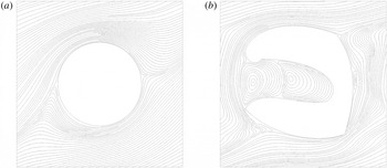
To analyse the behaviour at the interface, different descriptions are available, two of which are sketched in figure 9. The microscopic description relies on the pointwise calculation of flow and pressure fields, including the motion through the pores of the lower medium. The so-called mesoscopic approach is usually based on local volume-averaged equations which are assumed valid throughout the domain; a diffuse interface layer of
 $O(l)$
thickness appears. This approach is also called the one-domain approach and requires knowledge of how effective properties (porosity, permeability, etc.) vary as the dividing surface is crossed. In the macroscopic description the interface layer becomes infinitely thin; it is positioned at
 ${\hat{Y}}=0$
and slip occurs there. This is also sometimes referred to as the two-domain approach, with Stokes or Navier–Stokes equations governing the free-fluid region, and homogenized equations (Darcy, Forchheimer, etc.) in the porous medium.
(a) Microscopic and (b) mesoscopic descriptions of the porous/fluid transition region. Characteristic velocity and length scales are indicated within each region; the symbols
 $\oplus$
and
 $\ominus$
are used further on (§ 7) to denote interfacial and porous regions where the pressure scale is
 $\unicode[STIX]{x1D707}{\mathcal{U}}/l$
.

Analytical techniques to evaluate the slip velocity usually start from the equations at the mesoscopic level, i.e. focussing on a neighbourhood of the diffuse interface layer. For example, Saffman (Reference Saffman1971) justified theoretically the empirical condition by Beavers & Joseph (Reference Beavers and Joseph1967) by first ensemble averaging the Stokes equation across the porous/fluid domain and then performing asymptotic matching at the edge of the interface layer. Retaining terms up to second order in
 $\unicode[STIX]{x1D716}$
in Saffman’s development the slip velocity turns out to be
 $$\begin{eqnarray}\hat{U} _{s}=\unicode[STIX]{x1D716}\hat{\unicode[STIX]{x1D706}}_{x}\frac{\unicode[STIX]{x2202}\hat{U} }{\unicode[STIX]{x2202}{\hat{Y}}}\biggm\vert_{{\hat{Y}}\rightarrow 0^{+}}\;-\;\unicode[STIX]{x1D716}^{2}\frac{{\mathcal{K}}BL^{2}}{\unicode[STIX]{x1D707}}\frac{\text{d}\hat{p}^{(0)}}{\text{d}\hat{X}}.\end{eqnarray}$$
Here,
 $B$
is a constant of order one which can be determined by the structure of the convolution kernel introduced by Saffman to express the mean force per unit volume exerted by the fluid on the porous medium, as a function of the velocity in the interface layer. For
 $B$
equal to one, Beavers and Joseph’s semi-empirical relation is recovered exactly.
Saffman argued that the inclusion of the
 $\unicode[STIX]{x1D716}^{2}$
term in (3.3) is not necessary if the goal of the study is the determination of the total flow rate through the channel; this is the case since there is an unknown excess flow rate of order
 $\unicode[STIX]{x1D716}^{2}$
within the interfacial layer (product of a velocity of order
 $\unicode[STIX]{x1D716}$
times a thickness of the same order) and it is thus of little use to estimate
 $\hat{U} _{s}$
up to
 $\unicode[STIX]{x1D716}^{2}$
if the excess flow rate is unavailable anyhow. A detailed calculation of the velocity in the interface layer would permit the evaluation of the excess flow rate, in which case one would need also to estimate
 $\hat{U} _{s}$
up to order
 $\unicode[STIX]{x1D716}^{2}$
. Furthermore, according to Saffman only the condition at leading order
 $$\begin{eqnarray}\hat{U} _{s}=\unicode[STIX]{x1D716}\hat{\unicode[STIX]{x1D706}}_{x}\frac{\unicode[STIX]{x2202}\hat{U} }{\unicode[STIX]{x2202}{\hat{Y}}}\biggm\vert_{{\hat{Y}}\rightarrow 0^{+}},\end{eqnarray}$$
is truly local, the
 $\unicode[STIX]{x1D716}^{2}$
correction being function of non-local effects. As such, Saffman’s argument goes, the ‘extra term retained by Beavers and Joseph is at best only true for one particular geometry’. Equation (3.4) coincides with Navier’s slip condition (2.1) with
 $\hat{\unicode[STIX]{x1D706}}_{x}$
a slip length whose determination requires knowledge of the parameter
 $\unicode[STIX]{x1D6FC}_{BJ}$
. Just like in Navier’s slip condition, the position where slip must be enforced is defined up to a constant shift of order
 $l$
. A perturbation of the interface position of order
 $l$
generates a perturbation in the solution for the mean speed of order
 $\unicode[STIX]{x1D716}^{2}$
times the Darcy velocity scale (Saffman Reference Saffman1971; Jäger & Mikelić Reference Jäger and Mikelić2009).
Another formal derivation of Navier’s condition at the dividing surface in the form (3.4) was given by Jäger & Mikelić (Reference Jäger and Mikelić2000) on the basis of homogenization theory. Their analysis started from the steady equations of motion in the free-fluid region (
 $0<{\hat{Y}}\leqslant 2L$
) and through the pores of the medium (
 ${\hat{Y}}<0$
), and proceeded via asymptotic expansion and averaging to recover the slip velocity at the dividing surface as an order-
 $\unicode[STIX]{x1D716}$
correction to the no-slip condition; the slip length arose from an auxiliary Stokes-like problem defined on a longitudinally periodic microscopic cell. Jäger and Mikelić did not provide analytical or numerical solutions to their auxiliary problem and focussed attention on issues of existence, uniqueness, regularity, asymptotic behaviour and convergence of the microscopic solutions. Conversely, Lācis & Bagheri (Reference Lācis and Bagheri2017) placed emphasis on actual numerical results (and even rendered a software tool available, for anyone interested to compute effective parameters for her/his own microscopic problem). They used asymptotic homogenization to study the two-dimensional motion over and through an isotropic porous matrix, with the flow both tangent and normal to the Stokes–Darcy dividing line. The velocity components at such a dividing line were found to be
 $$\begin{eqnarray}\displaystyle & \displaystyle \hat{U} _{s}=\unicode[STIX]{x1D716}\hat{\unicode[STIX]{x1D706}}\left(\frac{\unicode[STIX]{x2202}\hat{U} }{\unicode[STIX]{x2202}{\hat{Y}}}+\frac{\unicode[STIX]{x2202}\hat{V}}{\unicode[STIX]{x2202}\hat{X}}\right)\biggm\vert_{{\hat{Y}}\rightarrow 0^{+}}\;-\;\unicode[STIX]{x1D716}^{2}\frac{{\mathcal{K}}^{itf}L^{2}}{\unicode[STIX]{x1D707}}\frac{\unicode[STIX]{x2202}\hat{p}^{(0)}}{\unicode[STIX]{x2202}\hat{X}}\biggm\vert_{{\hat{Y}}\rightarrow 0^{-}}, & \displaystyle\end{eqnarray}$$
 $$\begin{eqnarray}\displaystyle & \displaystyle \hat{V}|_{{\hat{Y}}=0}=-\unicode[STIX]{x1D716}^{2}\frac{{\mathcal{K}}L^{2}}{\unicode[STIX]{x1D707}}\frac{\unicode[STIX]{x2202}\hat{p}^{(0)}}{\unicode[STIX]{x2202}{\hat{Y}}}\biggm\vert_{{\hat{Y}}\rightarrow 0^{-}}. & \displaystyle\end{eqnarray}$$
The wall-normal velocity at
 ${\hat{Y}}=0$
is (trivially) equal to the Darcy velocity component, and this stems from mass conservation and the
 $\hat{X}$
-periodicity of the unit cell crossing the dividing line. The horizontal component of the velocity has a form similar to that by Beavers & Joseph (Reference Beavers and Joseph1967), with two differences:
(i) there is the extra strain term
 $\unicode[STIX]{x2202}\hat{V}/\unicode[STIX]{x2202}\hat{X}$
, whose existence had already been postulated by Nield (Reference Nield2009) also for the case of flat interfaces; and
(ii) an interface permeability
${\mathcal{K}}^{itf}$
appears (
${\mathcal{K}}^{itf}\neq {\mathcal{K}}$
).


Both the slip length
 $\hat{\unicode[STIX]{x1D706}}$
and the interface permeability
 ${\mathcal{K}}^{itf}$
result from the solution of microscopic problems over the unit cell across the interface. Lācis & Bagheri (Reference Lācis and Bagheri2017) solved such problems, and validated their interface coefficients by comparing macroscopic simulations, closed by the use of (3.5) and (3.6), to pointwise simulations which fully accounted for the flow through the pores of the domain in
 ${\hat{Y}}<0$
.
Before moving to the description of the asymptotic homogenization strategy used in the present paper, it is appropriate to mention a few further results which arise from a related upscaling technique, the so-called volume-averaging approach (Whitaker Reference Whitaker1999). Here the idea is to obtain the governing system at the macroscale by first averaging the microscale equations in space and then using approximations arising from scaling postulates. A very pedagogical comparison between multiscale asymptotic homogenization and volume averaging was provided by Davit et al. (Reference Davit, Bell, Byrne, Chapman, Kimpton, Lang, Leonard, Oliver, Pearson and Shipley2013). Using the latter strategy, Ochoa-Tapia & Whitaker (Reference Ochoa-Tapia and Whitaker1995a
,Reference Ochoa-Tapia and Whitaker
b
) addressed the problem of the fluid–porous interface by using the Darcy–Brinkman equation in the porous domain and Stokes’ equation in the fluid region; their momentum jump condition at a sharp surface of discontinuity in
 ${\hat{Y}}=0$
reads
 $$\begin{eqnarray}\hat{U} _{s}=\unicode[STIX]{x1D716}\frac{{\mathcal{K}}^{1/2}L}{\unicode[STIX]{x1D6FD}}\left[\frac{1}{\unicode[STIX]{x1D703}}\frac{\unicode[STIX]{x2202}\hat{U} ^{-}}{\unicode[STIX]{x2202}{\hat{Y}}}\biggm\vert_{{\hat{Y}}\rightarrow 0^{-}}\;-\;\frac{\unicode[STIX]{x2202}\hat{U} ^{+}}{\unicode[STIX]{x2202}{\hat{Y}}}\biggm\vert_{{\hat{Y}}\rightarrow 0^{+}}\right],\end{eqnarray}$$
with
 $\unicode[STIX]{x1D703}$
the porosity below the interface layer and
 $\unicode[STIX]{x1D6FD}$
a jump coefficient well approximated by
 $\unicode[STIX]{x1D6FD}=\unicode[STIX]{x1D703}^{-1/2}$
for the Darcy number
 $Da=\hat{{\mathcal{K}}}/L^{2}$
in the range
 $(10^{-10},10^{-7})$
(Valdés-Parada et al.
Reference Valdés-Parada, Alvarez-Ramírez, Goyeau and Ochoa-Tapia2009). This condition on
 $Da$
is rather restrictive, since it implies that
 $\unicode[STIX]{x1D716}$
is typically not larger than a number of order
 $10^{-4}$
; however, for larger values of
 $\unicode[STIX]{x1D716}$
the coefficient
 $\unicode[STIX]{x1D6FD}$
is available from the solution of a generalized momentum transport equation which holds across the interface (Valdés-Parada et al.
Reference Valdés-Parada, Alvarez-Ramírez, Goyeau and Ochoa-Tapia2009, Reference Valdés-Parada, Aguilar-Madera, Ochoa-Tapia and Goyeau2013).
An alternative derivation of the stress jump condition (Chandesris & Jamet Reference Chandesris and Jamet2007) by a matched asymptotic expansion method yields
 $$\begin{eqnarray}\hat{U} _{s}=\unicode[STIX]{x1D716}\frac{{\mathcal{K}}L}{\text{d}}\unicode[STIX]{x1D6FE}\left[\frac{\unicode[STIX]{x2202}\hat{U} ^{+}}{\unicode[STIX]{x2202}{\hat{Y}}}\biggm\vert_{{\hat{Y}}\rightarrow 0^{+}}\;-\;\frac{\unicode[STIX]{x2202}\hat{U} ^{-}}{\unicode[STIX]{x2202}{\hat{Y}}}\biggm\vert_{{\hat{Y}}\rightarrow 0^{-}}\right]-\unicode[STIX]{x1D716}^{2}\frac{L^{2}{\mathcal{K}}\unicode[STIX]{x1D70F}}{\unicode[STIX]{x1D707}}\frac{\text{d}\hat{p}^{(0)}}{\text{d}\hat{X}},\end{eqnarray}$$
with
 $\unicode[STIX]{x1D6FE}$
and
 $\unicode[STIX]{x1D70F}$
excess quantities of order one, related to jumps in porosity and permeability across the interface layer, and
 $\text{d}$
the dimensionless thickness of the layer (scaled by
 $l$
). Neglecting the term of order
 $\unicode[STIX]{x1D716}^{2}$
, condition (3.8) resembles, but does not coincide with, equation (3.7). A recent paper by Angot, Goyeau & Ochoa-Tapia (Reference Angot, Goyeau and Ochoa-Tapia2017) generalized the fluid–porous interface condition to multidimensional viscous flows, starting from the one-domain, volume-averaged description. Their condition reduced to some of the previously derived forms (in particular it reduced to (3.1) and (3.7) in some appropriate limits) for the case of unidirectional flow.
The last approach which deserves being cited is that by Le Bars & Worster (Reference Le Bars and Worster2006). These authors started from the mesoscopic Darcy–Brinkman formulation which stems from volume averaging. Provided that some length scale constraints were satisfied (Whitaker Reference Whitaker1996) the equations valid across both the fluid and the porous medium can be written with the velocity in either intrinsic average form (e.g. Breugem, Boersma & Uittenbogaard Reference Breugem, Boersma and Uittenbogaard2006; Luminari, Airiau & Bottaro Reference Luminari, Airiau and Bottaro2018) or in superficial average form (e.g. Le Bars & Worster Reference Le Bars and Worster2006). For the definition of the two averages, cf. (4.11) and (4.13); the distinction may seem minor at this point but in one case the volume-averaged velocity field is divergence-free and in the other it is not, except when the porosity is constant (a condition which does not hold across the dividing surface). It should also be noted that more than one form of the volume-averaged equations applicable across the interface appears in the literature, with variations related to the presence or absence of the porosity within some gradient terms or of nominally small terms (cf. discussions by Le Bars & Worster (Reference Le Bars and Worster2006) and Davit et al. (Reference Davit, Bell, Byrne, Chapman, Kimpton, Lang, Leonard, Oliver, Pearson and Shipley2013)). Following the approach by Le Bars & Worster (Reference Le Bars and Worster2006), the Darcy–Brinkman equation for the simple problem in figure 8 reads
 $$\begin{eqnarray}0=-\unicode[STIX]{x1D703}\frac{\text{d}\hat{p}^{(0)}}{\text{d}\hat{X}}+\unicode[STIX]{x1D707}\frac{\text{d}^{2}\langle \hat{U} \rangle }{\text{d}{\hat{Y}}^{2}}-\unicode[STIX]{x1D707}\unicode[STIX]{x1D703}\hat{{\mathcal{K}}}^{-1}\langle \hat{U} \rangle .\end{eqnarray}$$
All fields are continuous across the dividing line, including the porosity
 $\unicode[STIX]{x1D703}$
and the permeability
 $\hat{{\mathcal{K}}}$
, whose
 ${\hat{Y}}$
-variation must be prescribed. In the free-fluid region the porosity is equal to one and
 $\hat{{\mathcal{K}}}^{-1}$
vanishes, so that (3.9) reduces to Stokes’ equation. By a simple argument on the order of magnitude of the forces, Le Bars & Worster (Reference Le Bars and Worster2006) showed that Stokes’ equation remained valid below the dividing line up to a depth
 $\hat{\text{d}}$
of order
 $l$
. Thus, they simply suggested to impose continuity of the velocity vector at the position
 ${\hat{Y}}=-\hat{\text{d}}$
, with
 $\hat{\text{d}}=c\sqrt{\hat{{\mathcal{K}}}/\unicode[STIX]{x1D703}}$
and
 $c$
a constant of order one. Permeability and porosity in this expression must be evaluated deep within the porous matrix; the unknown constant
 $c$
should be assigned and there is no clear strategy on how to prescribe it. This is a drawback since the solution across the dividing line can vary substantially with even mild variations of
 $c$
. By carrying out simulations which capture the microscopic physics, Zampogna & Bottaro (Reference Zampogna and Bottaro2016) have shown the nonlinear increase of
 $c$
(and thus
 $\hat{\text{d}}$
) with the pore Reynolds number.
Despite the many contributions, the issue of the most appropriate strategy to treat the dividing surface is not yet convincingly settled, in particular because of the lack of validation against small-feature-resolving numerical and experimental results in non-trivial macroscopic settings for many of the proposed theoretical conditions. Our own adjoint strategy, reported in § 7, describes a mean to assign parameters in Saffman’s equation (3.3), limiting, for the moment, the validation exercise to a very simple flow configuration. Before getting there we must however cover some preliminary ground, starting from the description of the fluid flow in a homogeneous, porous matrix.
4 The flow in a porous medium
We consider the flow in a porous medium in regions away from boundaries. The assumption underlying the theory used throughout this paper is that the geometric features of the domain (pores and inclusions) repeat themselves regularly over a short spatial interval; furthermore, material properties (density, elasticity, etc., of both the fluid and the solid) must be periodic over the same spatial scale and the same must be true for the structural properties of the flow field through the pores of the medium. These assumptions permit us to define a representative volume element (RVE) which encapsulates all the small-scale properties of the problem, as well as those of the flow regime. In many cases the RVE coincides with the unit cell, the smallest building block over which cyclic boundary conditions can be enforced upon considerations of geometric and material periodicity alone.
To make the above clearer, examples of direct simulations of the flow in both a unit cell and in a cell whose size is doubled in both directions, under the same driving pressure gradient along the horizontal direction, are displayed in figure 10 for the case of a porous medium with staggered cylindrical inclusions. When the fluid within the pores moves slowly, so that the Stokes approximation is appropriate, the RVE and the unit cell coincide. When the flow displays inertial effects, i.e. with the presence of wakes behind the inclusions which interact with neighbouring inclusions, it becomes necessary to extend the size of the RVE beyond the unit cell. The size of the adequate RVE cannot be determined a priori and one needs to progressively enlarge the domain until properties averaged over the RVE become domain-size independent. When the flow through the medium is turbulent, there is some direct numerical simulation (Chu, Weigand & Vaikuntanathan Reference Chu, Weigand and Vaikuntanathan2018) and experimental (Evseev Reference Evseev2017) evidence which lends support to the pore-scale prevalence hypothesis, particularly as the porosity,
 $\unicode[STIX]{x1D703}$
decreases. This means that macroscopic eddies are not present because of the geometrical constraints imposed by the pores. In this case a relatively small RVE can be employed.
The case treated in figure 10 illustrates the above for the case of a two-dimensional flow with a relatively large value of the microscopic Reynolds number, defined further below, so that unsteadiness is maintained. Interestingly, the larger amplitude oscillations of the cell-averaged
 $u$
velocity component are found for the solution in the unit cell, whereas smaller oscillations appear when the computational domain is larger (grid density and time steps are the same in the two cases). This is possibly an effect of two-dimensionality. To appreciate the difference between the time-averaged solutions computed in the two domains it is useful to look at the difference between the time-averaged streamwise velocity fields (image on the right). Such a difference is relatively large (up to approximately
 $10\,\%$
of the maximum of
 $\overline{u}$
, overline indicates time average). Despite this, positive and negative variations cancel out in a way such that the time- and volume-averaged value of
 $u$
is very close in the two cases (it is
 $1.523$
for the case of the unit cell, and
 $1.532$
when the area of the domain is four times larger). The same small variation is found when examining the dimensionless effective permeability of this isotropic medium (defined later in § 4.2): its value is
 $7.61\times 10^{-4}$
when computed in the unit cell case and
 $7.66\times 10^{-4}$
in the larger RVE.
Provided a sufficient separation of scale exists between the characteristic size
 $l$
of the RVE and the dimension
 $L$
of the macroscopic phenomenon whose effects we are focussing upon, multiscale homogenization can be applied. The goal of the next sections is to derive macroscopic equations containing effective coefficients which arise from the solution of auxiliary problems valid at the microscopic RVE level.
(a) Variation in time of the RVE-averaged streamwise velocity component for the flow through a staggered array of cylinders at
 $Re=2000$
(
 $Re$
is defined after (4.3)); the porosity is
 $\unicode[STIX]{x1D703}=0.9372$
. The black line corresponds to the solution in the unit cell; the red line refers to the solution in a
 $2\times 2$
RVE. (b) Isolines of the
 $u$
velocity component in the unit cell, after time averaging. (c) Isolines of the difference between the time-averaged
 $u$
field in the
 $2\times 2$
RVE and the time-averaged solution in the unit cell.

4.1 Recovering Darcy’s law
Let us consider an unbounded, rigid, porous medium saturated by an incompressible Newtonian fluid of constant density
 $\unicode[STIX]{x1D70C}$
and dynamic viscosity
 $\unicode[STIX]{x1D707}$
. The porous medium is assumed to be composed of a series of regular, spatially periodic cells of characteristic size
 $l$
such as the unit cell sketched in figure 10. The volume of the fluid domain is denoted
 ${\mathcal{V}}_{f}$
,
 ${\mathcal{V}}_{s}$
is the volume of the solid domain and the fluid–solid boundary is
 $\unicode[STIX]{x1D6E4}$
. We assume that the macroscopic pressure gradient is balanced by viscous diffusion at the pore scale, i.e.
 $$\begin{eqnarray}\frac{\unicode[STIX]{x0394}P}{L}=O\left(\frac{\unicode[STIX]{x1D707}\text{}\underline{u}}{l^{2}}\right),\end{eqnarray}$$
with
 $\text{}\underline{u}$
a microscopic velocity scale. The variables can be normalized with
 $l/\text{}\underline{u}$
,
 $l$
,
 $\text{}\underline{u}$
,
 $\unicode[STIX]{x0394}P=\unicode[STIX]{x1D707}\text{}\underline{u}L/l^{2}$
and
 $\unicode[STIX]{x1D707}\text{}\underline{u}/l^{2}$
for, respectively, time, length, velocity, pressure and volume forcing terms, yielding in the fluid domain the dimensionless system
 $$\begin{eqnarray}\displaystyle & \displaystyle \frac{\unicode[STIX]{x2202}u_{i}}{\unicode[STIX]{x2202}x_{i}}=0, & \displaystyle\end{eqnarray}$$
 $$\begin{eqnarray}\displaystyle & \displaystyle Re\left[\frac{\unicode[STIX]{x2202}u_{i}}{\unicode[STIX]{x2202}t}+u_{j}\frac{\unicode[STIX]{x2202}u_{i}}{\unicode[STIX]{x2202}x_{j}}\right]=-\frac{1}{\unicode[STIX]{x1D716}}\frac{\unicode[STIX]{x2202}p}{\unicode[STIX]{x2202}x_{i}}+\frac{\unicode[STIX]{x2202}^{2}u_{i}}{\unicode[STIX]{x2202}x_{j}^{2}}+f_{i}, & \displaystyle\end{eqnarray}$$
with
 $\unicode[STIX]{x1D716}=l/L\ll 1$
the ordering parameter necessary to indicate the relative importance of different terms,
 $Re=\unicode[STIX]{x1D70C}\text{}\underline{u}l/\unicode[STIX]{x1D707}$
the microscopic Reynolds number and
 $f_{i}$
the
 $i$
th component of a macroscopic volume force. Since the structure of the medium involves two characteristic length scales, we introduce the microscopic and the macroscopic variables,
 $x_{i}$
and
 $X_{i}=\unicode[STIX]{x1D716}x_{i}$
, for the chain rule to yield
 $$\begin{eqnarray}\frac{\unicode[STIX]{x2202}}{\unicode[STIX]{x2202}x_{i}}\rightarrow \frac{\unicode[STIX]{x2202}}{\unicode[STIX]{x2202}x_{i}}+\unicode[STIX]{x1D716}\frac{\unicode[STIX]{x2202}}{\unicode[STIX]{x2202}X_{i}}.\end{eqnarray}$$
Furthermore, each generic dependent variable
 $g$
is expanded in power series of
 $\unicode[STIX]{x1D716}$
as
 $$\begin{eqnarray}g(t,x_{i},X_{i})=g^{(0)}(t,x_{i},X_{i})+\unicode[STIX]{x1D716}g^{(1)}(t,x_{i},X_{i})+\cdots \,,\end{eqnarray}$$
so that, plugging into the balance equations (4.2) and (4.3) and collecting the two leading orders in
 $\unicode[STIX]{x1D716}$
, we have
 $$\begin{eqnarray}\displaystyle & \displaystyle \frac{\unicode[STIX]{x2202}u_{i}^{(0)}}{\unicode[STIX]{x2202}x_{i}}=0, & \displaystyle\end{eqnarray}$$
 $$\begin{eqnarray}\displaystyle & \displaystyle \frac{\unicode[STIX]{x2202}u_{i}^{(1)}}{\unicode[STIX]{x2202}x_{i}}+\frac{\unicode[STIX]{x2202}u_{i}^{(0)}}{\unicode[STIX]{x2202}X_{i}}=0, & \displaystyle\end{eqnarray}$$
 $$\begin{eqnarray}\displaystyle & \displaystyle \frac{\unicode[STIX]{x2202}p^{(0)}}{\unicode[STIX]{x2202}x_{i}}=0, & \displaystyle\end{eqnarray}$$
 $$\begin{eqnarray}\displaystyle & \displaystyle Re\left[\frac{\unicode[STIX]{x2202}u_{i}^{(0)}}{\unicode[STIX]{x2202}t}+u_{j}^{(0)}\frac{\unicode[STIX]{x2202}u_{i}^{(0)}}{\unicode[STIX]{x2202}x_{j}}\right]=-\frac{\unicode[STIX]{x2202}p^{(1)}}{\unicode[STIX]{x2202}x_{i}}-\frac{\unicode[STIX]{x2202}p^{(0)}}{\unicode[STIX]{x2202}X_{i}}+\frac{\unicode[STIX]{x2202}^{2}u_{i}^{(0)}}{\unicode[STIX]{x2202}x_{j}^{2}}+f_{i}^{(0)}. & \displaystyle\end{eqnarray}$$
Equation (4.8) yields
 $p^{(0)}=p^{(0)}(t,X_{i})$
, i.e. pressure at leading order does not vary along the microscale. Equation (4.9) can be further simplified upon assuming that inertia within the pores is negligible, e.g.
 $Re$
is at the most of order
 $\unicode[STIX]{x1D716}$
for the convective term to be lifted to higher order. This is the case for many porous media problems, characterized by slow flow and small pores. In this case (4.9) becomes
 $$\begin{eqnarray}0=-\frac{\unicode[STIX]{x2202}p^{(1)}}{\unicode[STIX]{x2202}x_{i}}-\frac{\unicode[STIX]{x2202}p^{(0)}}{\unicode[STIX]{x2202}X_{i}}+\frac{\unicode[STIX]{x2202}^{2}u_{i}^{(0)}}{\unicode[STIX]{x2202}x_{j}^{2}}+f_{i}^{(0)},\end{eqnarray}$$
to be solved together with (4.6), subject to the no-slip condition on the fluid–grain interface
 $\unicode[STIX]{x1D6E4}$
and periodicity on opposite lateral boundaries of the unit cell.
The procedure at this point requires the introduction of an averaging operator over the unit cell of total volume
 ${\mathcal{V}}={\mathcal{V}}_{f}+{\mathcal{V}}_{s}$
, plus an inner product, defined respectively as
 $$\begin{eqnarray}\displaystyle & \displaystyle \langle a\rangle :=\frac{1}{{\mathcal{V}}}\int _{{\mathcal{V}}_{f}}a\,\text{d}{\mathcal{V}}, & \displaystyle\end{eqnarray}$$
 $$\begin{eqnarray}\displaystyle & \displaystyle (b,c):=\frac{1}{{\mathcal{V}}}\int _{{\mathcal{V}}_{f}}bc\,\text{d}{\mathcal{V}}, & \displaystyle\end{eqnarray}$$
with
 $a,b$
and
 $c$
real functions of the microscale variables. Equation (4.11) is also called the superficial or phase average, and the porosity of the medium can thus be written as
 $\unicode[STIX]{x1D703}={\mathcal{V}}_{f}/{\mathcal{V}}=\langle 1\rangle$
. Furthermore, if for example
 $c=1$
, it is
 $(b,c)=\langle b\rangle$
. A second averaging operation can be introduced, the intrinsic average, defined by
 $$\begin{eqnarray}\langle a\rangle ^{f}:=\frac{1}{{\mathcal{V}}_{f}}\int _{{\mathcal{V}}_{f}}a\,\text{d}{\mathcal{V}}=\unicode[STIX]{x1D703}^{-1}\langle a\rangle .\end{eqnarray}$$
Thus, for example, the mean pressure in the porous medium is
 $\langle p\rangle =\unicode[STIX]{x1D703}p^{(0)}+\unicode[STIX]{x1D716}\langle p^{(1)}\rangle +\cdots \,$
, and the mean interstitial pressure (or pore pressure) is
 $\langle p\rangle ^{f}=p^{(0)}+\unicode[STIX]{x1D716}\langle p^{(1)}\rangle ^{f}+\cdots \,$
.
We now sum the inner product (4.12) of equations (4.6) and (4.10) with two test functions, respectively
 $p^{\dagger }$
and
 $u_{i}^{\dagger }$
, i.e.
 $$\begin{eqnarray}0=\left(p^{\dagger },\frac{\unicode[STIX]{x2202}u_{i}^{(0)}}{\unicode[STIX]{x2202}x_{i}}\right)+\left(u_{i}^{\dagger },-\frac{\unicode[STIX]{x2202}p^{(1)}}{\unicode[STIX]{x2202}x_{i}}-\frac{\unicode[STIX]{x2202}p^{(0)}}{\unicode[STIX]{x2202}X_{i}}+\frac{\unicode[STIX]{x2202}^{2}u_{i}^{(0)}}{\unicode[STIX]{x2202}x_{j}^{2}}+f_{i}^{(0)}\right).\end{eqnarray}$$
The multidimensional equivalent of integration by parts stems from Gauss’ theorem and is known as the Lagrange–Green identity; for a term of the form
 $a\unicode[STIX]{x2202}b/\unicode[STIX]{x2202}x_{i}$
, the volume integral may be written as
 $$\begin{eqnarray}\int _{{\mathcal{V}}}a\frac{\unicode[STIX]{x2202}b}{\unicode[STIX]{x2202}x_{i}}\,\text{d}{\mathcal{V}}=\int _{\unicode[STIX]{x2202}{\mathcal{V}}}abn_{i}\,\text{d}A-\int _{{\mathcal{V}}}\frac{\unicode[STIX]{x2202}a}{\unicode[STIX]{x2202}x_{i}}b\,\text{d}{\mathcal{V}},\end{eqnarray}$$
with
 $\unicode[STIX]{x2202}{\mathcal{V}}$
the surface of the volume
 ${\mathcal{V}}$
and
 $n_{i}$
the
 $i$
th component of the outward normal vector
 $\boldsymbol{n}$
. Applying this transformation as many times as needed to every derivative in (4.14) we obtain the identity
 $$\begin{eqnarray}\left(\frac{\unicode[STIX]{x2202}u_{i}^{\dagger }}{\unicode[STIX]{x2202}x_{i}},p^{(1)}\right)+\left(-\frac{\unicode[STIX]{x2202}p^{\dagger }}{\unicode[STIX]{x2202}x_{i}}+\frac{\unicode[STIX]{x2202}^{2}u_{i}^{\dagger }}{\unicode[STIX]{x2202}x_{j}^{2}},u_{i}^{(0)}\right)=\left(u_{i}^{\dagger },\frac{\unicode[STIX]{x2202}p^{(0)}}{\unicode[STIX]{x2202}X_{i}}-f_{i}^{(0)}\right),\end{eqnarray}$$
using periodic boundary conditions on the outer boundaries of the unit cell for all test functions, and zero value for
 $u_{i}^{\dagger }$
at the fluid/grain interface
 $\unicode[STIX]{x1D6E4}$
. The variables
 $p^{\dagger }$
and
 $u_{i}^{\dagger }$
are called adjoint variables, and are defined so as to satisfy in the unit cell the microscopic (or auxiliary) problem which follows:
 $$\begin{eqnarray}\frac{\unicode[STIX]{x2202}u_{i}^{\dagger (k)}}{\unicode[STIX]{x2202}x_{i}}=0;\quad -\frac{\unicode[STIX]{x2202}p^{\dagger (k)}}{\unicode[STIX]{x2202}x_{i}}+\frac{\unicode[STIX]{x2202}^{2}u_{i}^{\dagger (k)}}{\unicode[STIX]{x2202}x_{j}^{2}}=-\unicode[STIX]{x1D6FF}_{ki},\end{eqnarray}$$
with
 $\unicode[STIX]{x1D6FF}_{ki}$
the Kronecker delta. This system has to be solved for
 $k=1,2$
and
 $3$
, i.e. with
 $-\unicode[STIX]{x1D6FF}_{1i}$
,
 $-\unicode[STIX]{x1D6FF}_{2i}$
and
 $-\unicode[STIX]{x1D6FF}_{3i}$
as successive source terms for the second equation in (4.17), and each resolution yields a specific, unique
 $u_{i}^{\dagger (k)}$
field. It is important to stress the point that the superscript
 $(k)$
in the adjoint variables’ names does not denote an asymptotic order (as it does for the case of the direct variables), but denotes the row of the matrix, e.g.
 $u_{i}^{\dagger (k)}=A_{ki}$
. Thus, for example, the first system of (4.17), for
 $k=1$
, reads
 $$\begin{eqnarray}\displaystyle & \displaystyle \frac{\unicode[STIX]{x2202}A_{11}}{\unicode[STIX]{x2202}x_{1}}+\frac{\unicode[STIX]{x2202}A_{12}}{\unicode[STIX]{x2202}x_{2}}+\frac{\unicode[STIX]{x2202}A_{13}}{\unicode[STIX]{x2202}x_{3}}=0, & \displaystyle\end{eqnarray}$$
 $$\begin{eqnarray}\displaystyle & \displaystyle -\frac{\unicode[STIX]{x2202}p^{\dagger (1)}}{\unicode[STIX]{x2202}x_{1}}+\frac{\unicode[STIX]{x2202}^{2}A_{11}}{\unicode[STIX]{x2202}x_{j}^{2}}=-1, & \displaystyle\end{eqnarray}$$
 $$\begin{eqnarray}\displaystyle & \displaystyle -\frac{\unicode[STIX]{x2202}p^{\dagger (1)}}{\unicode[STIX]{x2202}x_{2}}+\frac{\unicode[STIX]{x2202}^{2}A_{12}}{\unicode[STIX]{x2202}x_{j}^{2}}=0, & \displaystyle\end{eqnarray}$$
 $$\begin{eqnarray}\displaystyle & \displaystyle -\frac{\unicode[STIX]{x2202}p^{\dagger (1)}}{\unicode[STIX]{x2202}x_{3}}+\frac{\unicode[STIX]{x2202}^{2}A_{13}}{\unicode[STIX]{x2202}x_{j}^{2}}=0. & \displaystyle\end{eqnarray}$$
Using (4.16), the cell-averaged velocity along the generic direction
 $k$
reads
 $\langle u_{k}^{(0)}\rangle =-(u_{i}^{\dagger (k)},(\unicode[STIX]{x2202}p^{(0)}/\unicode[STIX]{x2202}X_{i})-f_{i}^{(0)})$
. Assuming that
 $f_{i}^{(0)}$
is either a constant or a function of only the macroscale variables, the seepage velocity
 $\langle u_{k}^{(0)}\rangle$
can thus be written as
 $$\begin{eqnarray}\langle u_{k}^{(0)}\rangle =-{\mathcal{K}}_{ki}\left[\frac{\unicode[STIX]{x2202}p^{(0)}}{\unicode[STIX]{x2202}X_{i}}-f_{i}^{(0)}\right],\end{eqnarray}$$
with
 $$\begin{eqnarray}{\mathcal{K}}_{ki}=\langle u_{i}^{\dagger (k)}\rangle =\langle A_{ki}\rangle ,\end{eqnarray}$$
the medium permeability which is unique, symmetric and positive definite (Mei & Vernescu Reference Mei and Vernescu2010). Equation (4.22) is the classical Darcy equation which expresses the phase-averaged velocity as a function of the pore pressure gradient. The permeability is available from geometrical microscopic properties alone. A similar derivation of Darcy’s law was given for the first time by Ene & Sanchez-Palencia (Reference Ene and Sanchez-Palencia1975). The cell average of (4.7) yields
 $$\begin{eqnarray}\left\langle \frac{\unicode[STIX]{x2202}u_{i}^{(0)}}{\unicode[STIX]{x2202}X_{i}}\right\rangle =0,\end{eqnarray}$$
on account of periodicity. The spatial-averaging theorem (see, e.g. Mei & Vernescu Reference Mei and Vernescu2010) permits the interchange of integration with respect to
 $x_{i}$
and differentiation with respect to
 $X_{i}$
, thanks to the no-slip condition, so that the continuity equation to be coupled to (4.22) is
 $$\begin{eqnarray}\frac{\unicode[STIX]{x2202}\langle u_{i}^{(0)}\rangle }{\unicode[STIX]{x2202}X_{i}}=0.\end{eqnarray}$$
For the two-dimensional porous medium drawn in figure 10, the first component of the permeability is shown in figure 11, as a function of the porosity
 $\unicode[STIX]{x1D703}$
of the medium. The second diagonal component,
 ${\mathcal{K}}_{22}$
, is identical to the first, from the symmetry properties of the medium, and the off-diagonal components vanish. This simple example thus corresponds to the case of an isotropic medium, for which
 ${\mathcal{K}}_{ij}={\mathcal{K}}\unicode[STIX]{x1D6FF}_{ij}$
.
First component of the permeability as a function of porosity for a porous medium formed by staggered cylinders. With this geometrical arrangement, the porosity must be larger than
 $\unicode[STIX]{x1D703}_{min}=1-\unicode[STIX]{x03C0}/4=0.2146$
for the inclusions not to touch one another.

Note that if our goal had been to obtain the local velocity at some position
 $\boldsymbol{x}^{\prime }$
, instead of the phase average velocity, it would have been sufficient to replace the source term in (4.17b
) by
 $-\unicode[STIX]{x1D6FF}_{ki}\unicode[STIX]{x1D6FF}(\boldsymbol{x}-\boldsymbol{x}^{\prime })$
, to obtain
 $$\begin{eqnarray}u_{k}^{(0)}(\boldsymbol{x}^{\prime })=-{\mathcal{V}}\langle u_{i}^{\dagger (k)}\rangle \left[\frac{\unicode[STIX]{x2202}p^{(0)}}{\unicode[STIX]{x2202}X_{i}}-f_{i}^{(0)}\right].\end{eqnarray}$$
4.1.1 Conditions at the boundaries of the macroscopic porous domain
Darcy’s equation can be written in terms of the pore pressure at leading order by combining (4.22) and (4.25), to yield
 $$\begin{eqnarray}\frac{\unicode[STIX]{x2202}}{\unicode[STIX]{x2202}X_{k}}\left[{\mathcal{K}}_{ki}\left(\frac{\unicode[STIX]{x2202}p^{(0)}}{\unicode[STIX]{x2202}X_{i}}-f_{i}^{(0)}\right)\right]=0.\end{eqnarray}$$
Close to boundaries the assumption of spatial homogeneity drops and a boundary layer appears. For example, at a solid wall (say, placed on a plane of constant
 $Y$
) which bounds a porous, isotropic region, the non-penetration condition suggests imposing
 $\unicode[STIX]{x2202}P^{(0)}/\unicode[STIX]{x2202}Y=0$
. This ‘intuitive’ condition is confirmed by a boundary layer analysis, as indicated by Carraro, Marǔsić-Paloka & Mikelić (Reference Carraro, Marǔsić-Paloka and Mikelić2018).
Particular care must be used in treating the interface between a free-fluid region and a porous domain and the commonly employed condition of pressure continuity at the dividing surface (Ene & Sanchez-Palencia Reference Ene and Sanchez-Palencia1975; Lācis & Bagheri Reference Lācis and Bagheri2017) is an approximation which, according to Carraro et al. (Reference Carraro, Marǔsić-Paloka and Mikelić2018), is acceptable only for the case of isotropic porous media. Recently, Lācis et al. (Reference Lācis, Sudhakar, Pasche and Bagheri2019) have proposed a pressure jump condition obtained from a normal-momentum balance through the dividing surface; this condition, briefly described later in § 7.1.2, extends and complements that proposed by previous researchers.
4.2 The effect of inertia through the pores
With increasing flow rate through the pores, nonlinear interactions lead to unsteadiness and eventually turbulence, even when the driving pressure gradient
 $\unicode[STIX]{x2202}p^{(0)}/\unicode[STIX]{x2202}X_{i}$
is maintained constant in time. The transition from creeping flow to inertia-dominated flow is typically quantified by the Reynolds number,
 $Re$
, although it is well known that the value of the transition Reynolds number is not unique, and depends strongly on the structure of the medium and the flow direction. Pauthenet et al. (Reference Pauthenet, Davit, Quintard and Bottaro2018) have recently used volume averaging to identify a unique transition Reynolds number, based on a length scale which depends both on the medium permeability and a tortuosity coefficient. Typically the inertial transition occurs for
 $Re=O(1)$
, in which case the left-hand side of (4.9) cannot be ignored. Before addressing the full equations, it is instructive to take a brief detour to analyse the role of the time variable on a model linear problem.
4.2.1 Properties of the adjoint function of a linear, parabolic problem
Let us consider the function space of all real continuous functions
 $f(t)$
defined over
 $0\leqslant t\leqslant T$
. The inner product between functions in this space can be defined by
 $$\begin{eqnarray}f_{1}\cdot f_{2}:=\int _{0}^{T}f_{1}(t)f_{2}(t)\,\text{d}t.\end{eqnarray}$$
Given a parabolic, linear equation, to be integrated from
 $t=0$
to
 $t=T$
and defined in terms of the operator
 ${\mathcal{L}}$
as
 $$\begin{eqnarray}\frac{\text{d}f}{\text{d}t}={\mathcal{L}}f+S,\end{eqnarray}$$
with
 $S$
a source term, it is possible to introduce the adjoint equation, to be integrated backwards, i.e. proceeding from
 $t=T$
to
 $t=0$
, as
 $$\begin{eqnarray}-\frac{\text{d}f^{\dagger }}{\text{d}t}={\mathcal{L}}^{\dagger }f^{\dagger },\end{eqnarray}$$
with the property that
 $$\begin{eqnarray}f(T)f^{\dagger }(T)=f(0)f^{\dagger }(0)+S\cdot f^{\dagger }.\end{eqnarray}$$
The above stems immediately from the defining property of adjoint operators, i.e.
 $$\begin{eqnarray}{\mathcal{L}}f\cdot f^{\dagger }=f\cdot {\mathcal{L}}^{\dagger }f^{\dagger }.\end{eqnarray}$$
The adjoint function
 $f^{\dagger }$
plays the role of a Green’s function for equation (4.29) for, if we integrate (4.30) using
 $f^{\dagger }(T)=1$
as the terminal condition, the direct solution at the generic final time
 $t=T$
is simply
 $$\begin{eqnarray}f(T)=f(0)f^{\dagger }(0)+S\cdot f^{\dagger }.\end{eqnarray}$$
In other words, once the adjoint solution, viz. the Green’s function,
 $f^{\dagger }(t)$
, is available, the final direct solution
 $f(T)$
is found by simply multiplying the Green’s function at
 $t=0$
with any initial condition
 $f(0)$
, and summing this to the inner product of
 $f^{\dagger }(t)$
with any source term,
 $S$
, of the direct equation. The extension to multidimensional problems is straightforward and is addressed below on the actual problem of interest.
4.2.2 Adjoint of the nonlinear time-dependent, microscopic equations
The adjoint system of equations (4.6) and (4.9) can be derived in a similar manner as in the linear case, carrying out integrations in both space and time. The time integral must run from the initial time, set arbitrarily to 0, to a generic final time,
 $T$
. After a few integrations by parts it is simple to find
 $$\begin{eqnarray}\displaystyle & & \displaystyle \int _{0}^{T}\left(\frac{\unicode[STIX]{x2202}u_{i}^{\dagger }}{\unicode[STIX]{x2202}x_{i}},p^{(1)}\right)+\left(Re\left[\frac{\unicode[STIX]{x2202}u_{i}^{\dagger }}{\unicode[STIX]{x2202}t}+u_{j}^{(0)}\frac{\unicode[STIX]{x2202}u_{i}^{\dagger }}{\unicode[STIX]{x2202}x_{j}}\right]-\frac{\unicode[STIX]{x2202}p^{\dagger }}{\unicode[STIX]{x2202}x_{i}}+\frac{\unicode[STIX]{x2202}^{2}u_{i}^{\dagger }}{\unicode[STIX]{x2202}x_{j}^{2}},u_{i}^{(0)}\right)\,\text{d}t\nonumber\\ \displaystyle & & \displaystyle \quad =\int _{0}^{T}\left(u_{i}^{\dagger },\frac{\unicode[STIX]{x2202}p^{(0)}}{\unicode[STIX]{x2202}X_{i}}-f_{i}^{(0)}\right)\,\text{d}t+(u_{i}^{\dagger },u_{i}^{(0)})|_{t=0}^{t=T}.\end{eqnarray}$$
The auxiliary problem to be solved with periodicity at the boundaries of the RVE and no-slip at the fluid/grain contact surfaces reads
 $$\begin{eqnarray}\frac{\unicode[STIX]{x2202}u_{i}^{\dagger (k)}}{\unicode[STIX]{x2202}x_{i}}=0;\quad -Re\left[\frac{\unicode[STIX]{x2202}u_{i}^{\dagger (k)}}{\unicode[STIX]{x2202}t}+u_{j}^{(0)}\frac{\unicode[STIX]{x2202}u_{i}^{\dagger (k)}}{\unicode[STIX]{x2202}x_{j}}\right]=-\frac{\unicode[STIX]{x2202}p^{\dagger (k)}}{\unicode[STIX]{x2202}x_{i}}+\frac{\unicode[STIX]{x2202}^{2}u_{i}^{\dagger (k)}}{\unicode[STIX]{x2202}x_{j}^{2}}+S_{ki}^{\dagger },\end{eqnarray}$$
with the source term
 $S_{ki}^{\dagger }$
equal to the Kronecker delta,
 $\unicode[STIX]{x1D6FF}_{ki}$
, if the problem is steady, and
 $S_{ki}^{\dagger }=0$
in a time-dependent problem. In this latter case, the terminal conditions at
 $t=T$
for the adjoint problem will need to be defined. As before, the superscript
 $(k)$
in the adjoint variables in (4.35) stems from the need to define and solve three different auxiliary problems,
 $k=1,2$
and 3, for each of the velocity components.
The steady problem
The adjoint momentum equation is simply
 $$\begin{eqnarray}-Re\,u_{j}^{(0)}\frac{\unicode[STIX]{x2202}u_{i}^{\dagger (k)}}{\unicode[STIX]{x2202}x_{j}}=-\frac{\unicode[STIX]{x2202}p^{\dagger (k)}}{\unicode[STIX]{x2202}x_{i}}+\frac{\unicode[STIX]{x2202}^{2}u_{i}^{\dagger (k)}}{\unicode[STIX]{x2202}x_{j}^{2}}+\unicode[STIX]{x1D6FF}_{ki},\end{eqnarray}$$
and the resulting macroscopic problem reads
 $$\begin{eqnarray}\langle u_{k}^{(0)}\rangle =-{\mathcal{K}}_{ki}^{eff}\left[\frac{\unicode[STIX]{x2202}p^{(0)}}{\unicode[STIX]{x2202}X_{i}}-f_{i}^{(0)}\right],\end{eqnarray}$$
with
 $$\begin{eqnarray}{\mathcal{K}}_{ki}^{eff}=\langle u_{i}^{\dagger (k)}\rangle .\end{eqnarray}$$
The resulting macroscale equation (4.37) is the same as in the creeping flow case (i.e. the Darcy equation (4.22)), but now the adjoint variables (and consequently the permeability) do not depend only on the geometric small-scale properties of the porous medium, but also on the direct flow state; the permeability is thus called effective (or apparent) and noted with the superscript
 $^{eff}$
. As opposed to the Stokes permeability of equation (4.23), the apparent permeability tensor is in general not symmetric; Lasseux & Valdés-Parada (Reference Lasseux and Valdés-Parada2017) have shown that it can be decomposed into the sum of a symmetric and a skew-symmetric part, the latter component originating from inertial transport. Resolution of (4.36) is indispensable to obtain all components of the apparent permeability tensor, for any given macroscopic forcing
 $\unicode[STIX]{x2202}p^{(0)}/\unicode[STIX]{x2202}X_{i}-f_{i}^{(0)}$
. For simplicity, from now on, the
 $f_{i}^{(0)}$
volumetric force will be taken conservative and absorbed into the pressure gradient term.
The unsteady problem
Because of the minus sign in front of the first term of the adjoint momentum equation in (4.35), and the presence of a positive diffusion term on the right-hand side, the only stable direction of evolution for the equation is for time
 $t$
running from
 $T$
to 0. It is then convenient to introduce the time variable
 $\unicode[STIX]{x1D70F}=T-t$
, which runs from
 $\unicode[STIX]{x1D70F}=0$
to
 $\unicode[STIX]{x1D70F}=T$
, for the equation to read
 $$\begin{eqnarray}Re\left[\frac{\unicode[STIX]{x2202}u_{i}^{\dagger (k)}}{\unicode[STIX]{x2202}\unicode[STIX]{x1D70F}}-u_{j}^{(0)}\frac{\unicode[STIX]{x2202}u_{i}^{\dagger (k)}}{\unicode[STIX]{x2202}x_{j}}\right]=-\frac{\unicode[STIX]{x2202}p^{\dagger (k)}}{\unicode[STIX]{x2202}x_{i}}+\frac{\unicode[STIX]{x2202}^{2}u_{i}^{\dagger (k)}}{\unicode[STIX]{x2202}x_{j}^{2}}.\end{eqnarray}$$
From (4.34) we are left with
 $$\begin{eqnarray}0=\int _{0}^{T}\left(u_{i}^{\dagger (k)},\frac{\unicode[STIX]{x2202}p^{(0)}}{\unicode[STIX]{x2202}X_{i}}\right)\,\text{d}t+(u_{i}^{\dagger (k)},u_{i}^{(0)})|_{t=0}^{t=T};\end{eqnarray}$$
as initial condition for the adjoint variable at
 $\unicode[STIX]{x1D70F}=0$
we can choose either

With the first choice we recover the phase-averaged velocity at any final time
 $t=T$
, whereas the second choice yields the instantaneous, pointwise velocity distribution in the RVE. In other words, choice 1 yields
 $$\begin{eqnarray}\langle u_{k}^{(0)}\rangle |_{t=T}=(u_{i}^{\dagger (k)},u_{i}^{(0)})|_{t=0}-\int _{0}^{T}{\mathcal{K}}_{ki}^{eff}\frac{\unicode[STIX]{x2202}p^{(0)}}{\unicode[STIX]{x2202}X_{i}}\,\text{d}t,\end{eqnarray}$$
with
 ${\mathcal{K}}_{ki}^{eff}=\langle u_{i}^{\dagger (k)}\rangle$
the effective dynamic permeability, function of
 $\unicode[STIX]{x1D70F}=T-t$
. The last integral above is a convolution when the imposed pressure gradient is time dependent. Choice 2 gives
 $$\begin{eqnarray}u_{k}^{(0)}(T,\boldsymbol{x}^{\prime },\boldsymbol{X})={\mathcal{V}}(u_{i}^{\dagger (k)},u_{i}^{(0)})|_{t=0}-{\mathcal{V}}\int _{0}^{T}\left(u_{i}^{\dagger (k)},\frac{\unicode[STIX]{x2202}p^{(0)}}{\unicode[STIX]{x2202}X_{i}}\right)\,\text{d}t.\end{eqnarray}$$
Both choices illustrate nicely the fact that adjoint fields operate as Green’s functions, expressing the sensitivity to either the initial condition,
 $u_{i}^{(0)}|_{t=0}$
, or the source term,
 $\unicode[STIX]{x2202}p^{(0)}/\unicode[STIX]{x2202}X_{i}$
. In the study of the flow through porous or poroelastic media the average velocity is usually sought for, immediately available from choice 1. Recently, the problem of the unsteady seepage of fluid in a porous medium has been posed and solved by Lasseux, Valdés-Parada & Bellet (Reference Lasseux, Valdés-Parada and Bellet2019), within Whitaker’s (Reference Whitaker1996) volume-averaging framework.
4.2.3 Further considerations on the steady case
A microscopic problem similar to that given in equation (4.36) has been given previously by Whitaker (Reference Whitaker1996) in terms of two closure variables, noted below as
 $\boldsymbol{e}=\{e_{k}\}$
and
 $\boldsymbol{E}=\{E_{ik}\}$
. The most notable difference with Whitaker’s closure problem is that his stationary closure equations are
 $$\begin{eqnarray}\frac{\unicode[STIX]{x2202}E_{ik}}{\unicode[STIX]{x2202}x_{i}}=0,\quad Re\,u_{j}^{(0)}\frac{\unicode[STIX]{x2202}E_{ik}}{\unicode[STIX]{x2202}x_{j}}=-\frac{\unicode[STIX]{x2202}e_{k}}{\unicode[STIX]{x2202}x_{i}}+\frac{\unicode[STIX]{x2202}^{2}E_{ik}}{\unicode[STIX]{x2202}x_{j}^{2}}+\unicode[STIX]{x1D6FF}_{ik},\end{eqnarray}$$
with periodicity for
 $E_{ik}$
and
 $e_{k}$
on the cell boundary and zero value for
 $E_{ik}$
at
 $\unicode[STIX]{x1D6E4}$
; the effective permeability is
 $$\begin{eqnarray}{\mathcal{K}}_{ik}^{eff}=\langle E_{ik}\rangle .\end{eqnarray}$$
In other words, the advective term on the left-hand side of (4.44) contains
 $u_{j}^{(0)}$
, whereas it contains
 $-u_{j}^{(0)}$
in model (4.36). This apparent difference is easily understood upon closer scrutiny of the two models, which turn out to be simply the transpose of one another, as shown by Lasseux & Valdés-Parada (private communication, 2018). Upon solving with the adjoint formulation, for
 $k=p$
, with
 $p=1,2$
or
 $3$
, one recovers
 $K_{p1}^{eff}$
,
 $K_{p2}^{eff}$
and
 $K_{p3}^{eff}$
. Conversely, the solution of (4.44) yields for any
 $k=p$
:
 $K_{1p}^{eff}$
,
 $K_{2p}^{eff}$
and
 $K_{3p}^{eff}$
. The final entries of the apparent permeability tensor in the two cases are the same.
Streamlines of the steady, adjoint velocity field
 $u_{i}^{\dagger (1)}$
in the unit cell, built from the solution of (4.36) for
 $k=1$
, isotropic (a) and anisotropic (b) grains. The direct flow is driven diagonally (at
 $45^{\circ }$
) by a macroscopic pressure gradient in both cases.

To illustrate the above we consider two different types of inclusion within a two-dimensional unit cell. The first inclusion is cylindrical while the second is highly irregular, they are shown in figure 12. The direct fields in the two cases are computed by solving equations (4.6) and (4.9) (the latter in its steady form) in the periodic cell, subject to a pressure gradient inclined at
 $45^{\circ }$
with respect to the horizontal axis of the unit cell. In particular, in the first case (cylindrical grains with porosity of the medium
 $\unicode[STIX]{x1D703}=0.80$
) we take
 $\unicode[STIX]{x2202}p^{(0)}/\unicode[STIX]{x2202}X=\unicode[STIX]{x2202}p^{(0)}/\unicode[STIX]{x2202}Y=-74.32$
, and in the second (asymmetric inclusions with porosity
 $\unicode[STIX]{x1D703}=0.734$
) we take
 $\unicode[STIX]{x2202}p^{(0)}/\unicode[STIX]{x2202}X=\unicode[STIX]{x2202}p^{(0)}/\unicode[STIX]{x2202}Y=-639.4$
. In the symmetric case the microscopic Reynolds number is
 $Re=80.7$
while in the second case it is
 $782$
; the filtration velocity components in the two cases are
 $$\begin{eqnarray}\left.\begin{array}{@{}c@{}}\mathit{isotropic\;case}:~\langle u^{(0)}\rangle =\langle v^{(0)}\rangle =0.6666,\\ \mathit{anisotropic\;case}:~\langle u^{(0)}\rangle =0.8467,\quad \langle v^{(0)}\rangle =9.720\times 10^{-2}.\end{array}\right\}\end{eqnarray}$$
Once the direct fields are computed, they are used in (4.36) to obtain the adjoint velocity and pressure. When
 $k=1$
the adjoint velocity components are denoted by
 $u_{i}^{\dagger (1)}$
and from them we can draw adjoint streamlines, represented in figure 12 for the two configurations at hand. For the case of isotropic grains it is found through averaging:
 ${\mathcal{K}}_{11}^{eff}={\mathcal{K}}_{22}^{eff}=6.331\times 10^{-3}$
;
 ${\mathcal{K}}_{12}^{eff}={\mathcal{K}}_{21}^{eff}=2.635\times 10^{-3}$
. Using Darcy’s law with the apparent permeability tensor we thus have
 $$\begin{eqnarray}\langle u^{(0)}\rangle =\langle v^{(0)}\rangle =-{\mathcal{K}}_{11}^{eff}\frac{\unicode[STIX]{x2202}p^{(0)}}{\unicode[STIX]{x2202}X}-{\mathcal{K}}_{12}^{eff}\frac{\unicode[STIX]{x2202}p^{(0)}}{\unicode[STIX]{x2202}Y}=0.6665,\end{eqnarray}$$
in excellent agreement with the direct simulation result.
The irregular grain geometry produces the following result for the apparent permeability tensor:
 $$\begin{eqnarray}\left(\begin{array}{@{}cc@{}}8.65\times 10^{-4} & 4.59\times 10^{-4}\\ -1.71\times 10^{-4} & 3.23\times 10^{-4}\end{array}\right)\end{eqnarray}$$
while, for comparison purposes, the intrinsic (Stokes) permeability components
 ${\mathcal{K}}_{ki}$
are
 $$\begin{eqnarray}\left(\begin{array}{@{}cc@{}}5.53\times 10^{-3} & -2.25\times 10^{-4}\\ -2.25\times 10^{-4} & 6.71\times 10^{-3}\end{array}\right).\end{eqnarray}$$
Using Darcy equation with the effective permeability components we recover
 $$\begin{eqnarray}\displaystyle & \displaystyle \langle u^{(0)}\rangle =-{\mathcal{K}}_{11}^{eff}\frac{\unicode[STIX]{x2202}p^{(0)}}{\unicode[STIX]{x2202}X}-{\mathcal{K}}_{12}^{eff}\frac{\unicode[STIX]{x2202}p^{(0)}}{\unicode[STIX]{x2202}Y}=0.8466, & \displaystyle\end{eqnarray}$$
 $$\begin{eqnarray}\displaystyle & \displaystyle \langle v^{(0)}\rangle =-{\mathcal{K}}_{21}^{eff}\frac{\unicode[STIX]{x2202}p^{(0)}}{\unicode[STIX]{x2202}X}-{\mathcal{K}}_{22}^{eff}\frac{\unicode[STIX]{x2202}p^{(0)}}{\unicode[STIX]{x2202}Y}=9.720\times 10^{-2}, & \displaystyle\end{eqnarray}$$
which, again, agree very well with the results from the direct simulation.
The presence of an inertial term in the macroscopic Darcy equation can be made explicit by writing
 ${\mathcal{K}}_{ki}^{eff}$
as
 $$\begin{eqnarray}{\mathcal{K}}_{ki}^{eff}=({\mathcal{F}}_{jk}+\unicode[STIX]{x1D6FF}_{jk})^{-1}{\mathcal{K}}_{ji},\end{eqnarray}$$
with
 ${\mathcal{F}}_{jk}$
the non-symmetric,
 $u_{j}^{(0)}$
-dependent Forchheimer tensor; equation (4.37) then becomes the Darcy–Forchheimer equation (Whitaker Reference Whitaker1996)
 $$\begin{eqnarray}\langle u_{k}^{(0)}\rangle =-{\mathcal{K}}_{ki}\frac{\unicode[STIX]{x2202}p^{(0)}}{\unicode[STIX]{x2202}X_{i}}-{\mathcal{F}}_{ki}\langle u_{i}^{(0)}\rangle .\end{eqnarray}$$
Clearly, as
 $Re\rightarrow 0$
Darcy equation is recovered; when
 $Re$
increases, the so-called regime of weak inertia is entered and
 ${\mathcal{F}}_{ki}\langle u_{i}^{(0)}\rangle \sim \langle u_{k}^{(0)}\rangle \langle u_{i}^{(0)}\rangle \langle u_{i}^{(0)}\rangle$
(Mei & Auriault Reference Mei and Auriault1991; Firdaouss, Guermond & Le Quéré Reference Firdaouss, Guermond and Le Quéré1997). Upon further increasing
 $Re$
, the strong inertia regime is attained with
 ${\mathcal{F}}_{ki}\langle u_{i}^{(0)}\rangle$
proportional to the square of the seepage velocity (Whitaker Reference Whitaker1996; Lasseux, Abbasian Arani & Ahmadi Reference Lasseux, Abbasian Arani and Ahmadi2011). For yet larger values of the Reynolds numbers, the flow in the porous medium undergoes successive bifurcations, before transition to a turbulent state. The onset of unsteady motion within the pores of the medium depends on the geometry, the dimensions and the arrangement of the grains within the porous domain.
4.2.4 Possible solution strategies
In practical calculations, to account for the dependence of
 ${\mathcal{K}}_{ki}^{eff}$
on the microstate when convection terms are non-negligible, both direct and adjoint states are needed. For any given geometry of the inclusions, the parameters to be considered are the orientation of the driving pressure force and the local Reynolds number.
Extensive parametric calculations under steady conditions have been reported by Lasseux et al. (Reference Lasseux, Abbasian Arani and Ahmadi2011). The two-dimensional case was considered, with solid inclusions of either circular or square shape; interestingly, Lasseux et al. (Reference Lasseux, Abbasian Arani and Ahmadi2011) considered both ordered and disordered arrangements of grains, in the latter case also including grains of varying sizes (and this implied the use of periodic RVEs of rather large dimensions). For the case of ordered structures the Forchheimer tensor
 ${\mathcal{F}}_{jk}$
was found to be non-symmetric, except when the applied pressure gradient was directed along a symmetry axis of the representative elementary cell. This stems from the fact that, for an arbitrary orientation of
 $\unicode[STIX]{x2202}p^{(0)}/\unicode[STIX]{x2202}X_{i}$
, the force on the grain due to inertia is not necessarily aligned with the mean flow. Another interesting result was that the range of Reynolds numbers in which the weak inertia form of the Forchheimer equation occurred was more narrow when disordered structures were considered, possibly explaining why experiments with natural media often did not exhibit such a regime.
An alternative strategy, requiring consideration of only adjoint variables, has been proposed by Valdés-Parada, Lasseux & Bellet (Reference Valdés-Parada, Lasseux and Bellet2016). It consists in solving the system
 $$\begin{eqnarray}\frac{\unicode[STIX]{x2202}u_{i}^{\dagger (k)}}{\unicode[STIX]{x2202}x_{i}}=0;\quad Re\,u_{l}^{\dagger (j)}\frac{\unicode[STIX]{x2202}p^{(0)}}{\unicode[STIX]{x2202}X_{l}}\frac{\unicode[STIX]{x2202}u_{i}^{\dagger (k)}}{\unicode[STIX]{x2202}x_{j}}=-\frac{\unicode[STIX]{x2202}p^{\dagger (k)}}{\unicode[STIX]{x2202}x_{i}}+\frac{\unicode[STIX]{x2202}^{2}u_{i}^{\dagger (k)}}{\unicode[STIX]{x2202}x_{j}^{2}}+\unicode[STIX]{x1D6FF}_{ik},\end{eqnarray}$$
which holds since the microscopic equation
 $$\begin{eqnarray}u_{j}^{(0)}=-u_{l}^{\dagger (j)}\frac{\unicode[STIX]{x2202}p^{(0)}}{\unicode[STIX]{x2202}X_{l}},\end{eqnarray}$$
applies in the unit cell (Mei & Vernescu Reference Mei and Vernescu2010).
A less involved approximation consists in expressing the direct velocity field in the RVE as the sum of a mean part plus a periodic deviation of zero mean, i.e.
 $$\begin{eqnarray}u_{j}^{(0)}(x_{i},X_{i})=\langle u_{j}^{(0)}\rangle ^{f}(X_{i})+u_{j}^{\prime }(x_{i},X_{i})=\unicode[STIX]{x1D703}^{-1}\langle u_{j}^{(0)}\rangle (X_{i})+u_{j}^{\prime }(x_{i},X_{i}),\end{eqnarray}$$
and then neglecting the fluctuations, i.e. assuming
 $u_{j}^{(0)}=\unicode[STIX]{x1D703}^{-1}\langle u_{j}^{(0)}\rangle$
to replace the actual direct field in the microscopic problem (4.36) with its intrinsic average. The results of this Oseen-like procedure deteriorate as the Reynolds number increases, as shown in the representative results of figure 13 for the isotropic, regular medium sketched in the image, when compared to results obtained from the direct solver (labelled as ‘DNS’ in the figure). For
 $\unicode[STIX]{x1D703}=0.8$
and
 $Re=0$
the dimensionless permeability of the medium is
 $1.941\times 10^{-2}$
; as inertia becomes prominent the permeability decreases as initially shown by Edwards et al. (Reference Edwards, Shapiro, Bar-Yoseph and Shapira1990). The results by these authors are however numerically under-resolved; fine grid direct simulations, displayed with asterisks in the figure, yield slightly larger values of the apparent permeability component, particularly for
 $Re$
exceeding 100. Values identical to those of the direct solver, to within graphical accuracy, are found when solving (4.54). Conversely, the Oseen-like approach produces approximate results which almost coincide with those by Edwards et al. (Reference Edwards, Shapiro, Bar-Yoseph and Shapira1990) over the whole range of
 $Re$
examined.
Variation of the apparent permeability with the microscopic Reynolds number for a two-dimensional medium composed by regularly arranged circular grains.

Another possible approach to treat flows with inertial effects through porous media consists in creating a database of direct and adjoint states, possibly using a metamodel based on kriging interpolation, or any other suitable interpolation technique, to fill the data gaps which inevitably arise when discretizing a very large space of parameters, thus generating a look-up table of permeabilities to be employed, for example, when the pressure gradient changes intensity and/or direction, or when the porosity is not homogeneous. This approach has been followed by Luminari et al. (Reference Luminari, Airiau and Bottaro2018) for a medium formed by a three-dimensional staggered array of cylindrical fibres. Interestingly, for such a case the apparent permeability tensor remains strongly diagonally dominant, regardless of the orientation and intensity of the driving force, a fact which must be correlated to the transversely isotropic nature of the medium considered.
5 The flow in a poroelastic medium
Poroelasticity is a continuum theory which deals with the analysis of a porous medium formed by an elastic matrix which contains interconnected fluid-saturated pores. The presence of the fluid influences the mechanical properties of the solid material. Since the pores are fluid filled, the fluid acts as a stiffener for the material; when there is a gradient of pore pressure, the fluid exerts a stress on the solid skeleton, deforming it and leading to volumetric changes in the pores. This, is turn, affects the fluid pressure. The theory is thus concerned with the coupling between changes in solid stress and changes in fluid pressure. The two-way fluid–solid coupling occurs instantaneously in the so-called quasi-static approximation of poroelasticity, whereas this is not the case in the dynamic approximation, when elastic wave propagation is accounted for. Work in poroelasticity was initiated by Terzaghi (Reference Terzaghi1925), who conducted controlled experiments in a one-dimensional model of a fully saturated soil sample under a Heaviside step function load, to understand the behaviour of soil as a foundation material. From his laboratory experiments, Terzaghi derived a simple consolidation equation which turned out to be a special case of the full, three-dimensional quasi-static theory later formulated by Biot (Reference Biot1941). Subsequently, Biot (Reference Biot1956a ,Reference Biot b ) extended the theory to describe low- and high-frequency elastic waves propagating in a fluid-saturated porous medium. The principal applications pursued initially by researchers in the field were concerned with problems in hydrogeology, geomechanics and petroleum engineering; Wang (Reference Wang2000) gives a complete historical and scientific account of the linear theory as referred to those applications. Other studies of poroelasticity have been mostly concerned with biomechanics, for example with applications to the behaviour of the interstitial fluid contained within bones (Cowin Reference Cowin1999) or solid tumours (Netti et al. Reference Netti, Baxter, Boucher, Skalak and Jain1997). Our intent is to apply the theory of poroelasticity to the macroscopic description of the fluid motion over and through deformable, natural or functionalized, coatings and materials.
Biot (Reference Biot1941, Reference Biot1956a ,Reference Biot b ) obtained his equations using an averaging process conducted over what was later called the RVE, to extract effective material parameters. This is sometimes called the effective medium approach. Another technique capable to yield the same system of equations (Bowen Reference Bowen1982) is based on mixture theory, an approach which employs a density-weighted averaging procedure rather than integration over the volume of the RVE. Auriault & Sanchez-Palencia (Reference Auriault and Sanchez-Palencia1977) were the first to derive the quasi-static form of the equations of poroelasticity through the use of a two-scale homogenization approach. The same multiscale technique was later employed by Burridge & Keller (Reference Burridge and Keller1981) for the dynamic form of the equations. A similar upscaling procedure, by the use of adjoints, is pursued below, with a focus on poroelastic media away from boundaries.
Let us assume that the coupled fluid–solid problem undergoes a ‘fast’ process of characteristic (large) frequency
 $\unicode[STIX]{x1D627}$
. Using this frequency to normalize time in the fluid equations, we have
 $$\begin{eqnarray}\frac{\unicode[STIX]{x2202}u_{k}}{\unicode[STIX]{x2202}x_{k}}=0,\quad \left(\frac{\unicode[STIX]{x1D70C}_{f}l^{2}\unicode[STIX]{x1D627}}{\unicode[STIX]{x1D707}}\right)\frac{\unicode[STIX]{x2202}u_{i}}{\unicode[STIX]{x2202}t}+Re\,u_{j}\frac{\unicode[STIX]{x2202}u_{i}}{\unicode[STIX]{x2202}x_{j}}=-\frac{1}{\unicode[STIX]{x1D716}}\frac{\unicode[STIX]{x2202}p}{\unicode[STIX]{x2202}x_{i}}+\frac{\unicode[STIX]{x2202}^{2}u_{i}}{\unicode[STIX]{x2202}x_{j}^{2}},\end{eqnarray}$$
with the same scales as in the rigid case for length, velocity and pressure. Assuming small elastic deformations of the solid skeleton, and calling
 $\hat{\boldsymbol{V}}=\{\hat{V}_{i}\}$
the dimensional solid displacement vector, it is
 $$\begin{eqnarray}\unicode[STIX]{x1D70C}_{s}\frac{\unicode[STIX]{x2202}^{2}\hat{V}_{i}}{\unicode[STIX]{x2202}\hat{t}^{2}}=\frac{\unicode[STIX]{x2202}\hat{\unicode[STIX]{x1D70E}}_{ij}}{\unicode[STIX]{x2202}\hat{X}_{j}},\end{eqnarray}$$
with the solid stress tensor
 $\hat{\unicode[STIX]{x1D70E}}_{ij}$
defined by
 $\hat{\unicode[STIX]{x1D70E}}_{ij}=\hat{{\mathcal{C}}}_{ijkl}\hat{\unicode[STIX]{x1D700}}_{kl}(\hat{\boldsymbol{V}})$
.
 $\hat{{\mathcal{C}}}_{ijkl}=E{\mathcal{C}}_{ijkl}$
is the elasticity tensor, with
 $\hat{{\mathcal{C}}}_{ijkl}=\unicode[STIX]{x1D706}_{L}\unicode[STIX]{x1D6FF}_{ij}\unicode[STIX]{x1D6FF}_{kl}+G(\unicode[STIX]{x1D6FF}_{ik}\unicode[STIX]{x1D6FF}_{jl}+\unicode[STIX]{x1D6FF}_{il}\unicode[STIX]{x1D6FF}_{jk})$
,
 $\unicode[STIX]{x1D706}_{L}$
and
 $G$
are the Lamé constants, functions of the Young’s modulus,
 $E$
, and the Poisson’s ratio,
 $\unicode[STIX]{x1D708}_{P}$
, through
 $$\begin{eqnarray}\frac{\unicode[STIX]{x1D706}_{L}}{E}=\frac{\unicode[STIX]{x1D708}_{P}}{(1+\unicode[STIX]{x1D708}_{P})(1-2\unicode[STIX]{x1D708}_{P})}\quad \text{and}\quad \frac{G}{E}=\frac{1}{2(1+\unicode[STIX]{x1D708}_{P})}.\end{eqnarray}$$
The elasticity tensor has the following symmetry properties:
 $$\begin{eqnarray}{\mathcal{C}}_{ijkl}={\mathcal{C}}_{jikl}={\mathcal{C}}_{ijlk}={\mathcal{C}}_{klij}.\end{eqnarray}$$
We also define the dimensional strain tensor,
 $\hat{\unicode[STIX]{x1D700}}_{kl}(\hat{\boldsymbol{V}})$
, as
 $$\begin{eqnarray}\hat{\unicode[STIX]{x1D700}}_{kl}(\hat{\boldsymbol{V}})=\frac{1}{2}\left(\frac{\unicode[STIX]{x2202}\hat{V}_{k}}{\unicode[STIX]{x2202}\hat{X}_{l}}+\frac{\unicode[STIX]{x2202}\hat{V}_{l}}{\unicode[STIX]{x2202}\hat{X}_{k}}\right).\end{eqnarray}$$
At the interface
 $\unicode[STIX]{x1D6E4}$
between the elastic solid and the fluid, components of velocity and stress must be continuous
 $$\begin{eqnarray}\displaystyle & \displaystyle \hat{U} _{i}=\frac{\unicode[STIX]{x2202}\hat{V}_{i}}{\unicode[STIX]{x2202}\hat{t}}, & \displaystyle\end{eqnarray}$$
 $$\begin{eqnarray}\displaystyle & \displaystyle \left[-\hat{P}\unicode[STIX]{x1D6FF}_{ij}+\unicode[STIX]{x1D707}\left(\frac{\unicode[STIX]{x2202}\hat{U} _{i}}{\unicode[STIX]{x2202}\hat{X}_{j}}+\frac{\unicode[STIX]{x2202}\hat{U} _{j}}{\unicode[STIX]{x2202}\hat{X}_{i}}\right)\right]n_{j}=\hat{\unicode[STIX]{x1D70E}}_{ij}n_{j}, & \displaystyle\end{eqnarray}$$
with the unit normal vector
 $\boldsymbol{n}=\{n_{i}\}$
at the interface oriented from the solid into the fluid.
Inertia in the fluid is comparable to the microscopic viscous term provided the characteristic microscale is of the order of the thickness of the Stokes layer, i.e.
 $$\begin{eqnarray}l\sim \sqrt{\frac{\unicode[STIX]{x1D707}}{\unicode[STIX]{x1D70C}_{f}\unicode[STIX]{x1D627}}}.\end{eqnarray}$$
For ‘slow’ processes (when
 $\unicode[STIX]{x1D627}$
is sufficiently small) this cannot be the case: the Stokes layer thickness exceeds typical pore/grain dimensions and
 $\unicode[STIX]{x1D70C}_{f}\unicode[STIX]{x2202}\hat{\boldsymbol{U}}/\unicode[STIX]{x2202}\hat{t}$
is negligible compared to both viscous diffusion and macroscopic pressure gradient terms.
Inertia in the solid equilibrates variations of the stress at the macroscale when
 $L$
is of the order of the elastic wavelength
 $$\begin{eqnarray}L\sim \frac{1}{\unicode[STIX]{x1D627}}\sqrt{\frac{E}{\unicode[STIX]{x1D70C}_{s}}}.\end{eqnarray}$$
The expansion parameter
 $\unicode[STIX]{x1D716}$
of the multiple scale analysis to follow can thus be taken equal to
 $$\begin{eqnarray}\unicode[STIX]{x1D716}=\frac{l}{L}=\left(\frac{\unicode[STIX]{x1D70C}_{s}}{\unicode[STIX]{x1D70C}_{f}}\frac{\unicode[STIX]{x1D707}\unicode[STIX]{x1D627}}{E}\right)^{1/2}.\end{eqnarray}$$
If we consider, for example, an open-cell elastomeric foam saturated by water, we have
 $\unicode[STIX]{x1D70C}_{s}=10~\text{kg}~\text{m}^{-3}$
and
 $E=10^{5}~\text{Pa}$
, together with
 $\unicode[STIX]{x1D70C}_{f}=10^{3}~\text{kg}~\text{m}^{-3}$
and
 $\unicode[STIX]{x1D707}=10^{-3}~\text{Pa}~\text{s}$
, so that
 $\unicode[STIX]{x1D716}=10^{-5}\sqrt{\unicode[STIX]{x1D627}}$
(with
 $\unicode[STIX]{x1D627}$
in Hertz). At a frequency of 100 Hz, we thus have
 $l\sim 100~\unicode[STIX]{x03BC}\text{m}$
and
 $L\sim 1~\text{m}$
(
 $\unicode[STIX]{x1D716}=10^{-4}$
). Whether such length scales are realistic depends on the microstructure and the phenomenon under consideration, and should they not be, one might reconsider the normalization of the equations.
From (5.6) we infer that the displacement scale is of order
 $\text{}\underline{u}/\unicode[STIX]{x1D627}$
, so that the dimensionless variables can be written (and expanded) as
 $$\begin{eqnarray}\displaystyle \left.\begin{array}{@{}c@{}}\displaystyle x_{i}=\frac{\hat{X}_{i}}{l},\quad t=\unicode[STIX]{x1D627}\hat{t},\quad p=p^{(0)}+\unicode[STIX]{x1D716}p^{(1)}+\unicode[STIX]{x1D716}^{2}p^{(2)}+\cdots =\frac{\hat{P}}{\unicode[STIX]{x0394}P},\\ \displaystyle u_{i}=u_{i}^{(0)}+\unicode[STIX]{x1D716}u_{i}^{(1)}+\cdots =\frac{\unicode[STIX]{x1D707}}{\unicode[STIX]{x1D716}l\unicode[STIX]{x0394}P}\hat{U} _{i},\quad v_{i}=v_{i}^{(0)}+\unicode[STIX]{x1D716}v_{i}^{(1)}+\unicode[STIX]{x1D716}^{2}v_{i}^{(2)}+\cdots =\frac{\unicode[STIX]{x1D707}\unicode[STIX]{x1D627}}{\unicode[STIX]{x1D716}l\unicode[STIX]{x0394}P}\hat{V}_{i}.\end{array}\right\} & & \displaystyle \nonumber\\ \displaystyle & & \displaystyle\end{eqnarray}$$
In dimensionless terms, the microscopic strain tensor
 $\unicode[STIX]{x1D700}_{kl}(\boldsymbol{v})$
is
 $$\begin{eqnarray}\unicode[STIX]{x1D700}_{kl}(\boldsymbol{v})=\frac{1}{2}\left(\frac{\unicode[STIX]{x2202}v_{k}}{\unicode[STIX]{x2202}x_{l}}+\frac{\unicode[STIX]{x2202}v_{l}}{\unicode[STIX]{x2202}x_{k}}\right).\end{eqnarray}$$
Using
 $X_{i}=\unicode[STIX]{x1D716}x_{i}$
and (4.4), mass conservation for the fluid and the momentum equations for both fluid and solid read, at different orders in
 $\unicode[STIX]{x1D716}$
,
 $O(\unicode[STIX]{x1D716}^{-1})$
:
 $$\begin{eqnarray}\frac{\unicode[STIX]{x2202}p^{(0)}}{\unicode[STIX]{x2202}x_{i}}=0,\end{eqnarray}$$
 $O(\unicode[STIX]{x1D716}^{0})$
:
 $$\begin{eqnarray}\displaystyle & \displaystyle \frac{\unicode[STIX]{x2202}u_{k}^{(0)}}{\unicode[STIX]{x2202}x_{k}}=0, & \displaystyle\end{eqnarray}$$
 $$\begin{eqnarray}\displaystyle & \displaystyle \frac{\unicode[STIX]{x2202}u_{i}^{(0)}}{\unicode[STIX]{x2202}t}+Re\,u_{j}^{(0)}\frac{\unicode[STIX]{x2202}u_{i}^{(0)}}{\unicode[STIX]{x2202}x_{j}}=-\frac{\unicode[STIX]{x2202}p^{(1)}}{\unicode[STIX]{x2202}x_{i}}-\frac{\unicode[STIX]{x2202}p^{(0)}}{\unicode[STIX]{x2202}X_{i}}+\frac{\unicode[STIX]{x2202}^{2}u_{i}^{(0)}}{\unicode[STIX]{x2202}x_{j}^{2}}, & \displaystyle\end{eqnarray}$$
 $$\begin{eqnarray}\displaystyle & \displaystyle \frac{\unicode[STIX]{x2202}\unicode[STIX]{x1D70E}_{ij}^{(-1)}}{\unicode[STIX]{x2202}x_{j}}=\frac{\unicode[STIX]{x2202}}{\unicode[STIX]{x2202}x_{j}}[{\mathcal{C}}_{ijkl}\unicode[STIX]{x1D700}_{kl}(\boldsymbol{v}^{(0)})]=0, & \displaystyle\end{eqnarray}$$
 $O(\unicode[STIX]{x1D716}^{1})$
:
 $$\begin{eqnarray}\displaystyle & \displaystyle \frac{\unicode[STIX]{x2202}u_{k}^{(1)}}{\unicode[STIX]{x2202}x_{k}}+\frac{\unicode[STIX]{x2202}u_{k}^{(0)}}{\unicode[STIX]{x2202}X_{k}}=0, & \displaystyle\end{eqnarray}$$
 $$\begin{eqnarray}\displaystyle & \displaystyle \frac{\unicode[STIX]{x2202}\unicode[STIX]{x1D70E}_{ij}^{(0)}}{\unicode[STIX]{x2202}x_{j}}+\frac{\unicode[STIX]{x2202}\unicode[STIX]{x1D70E}_{ij}^{(-1)}}{\unicode[STIX]{x2202}X_{j}}=\frac{\unicode[STIX]{x2202}}{\unicode[STIX]{x2202}x_{j}}\{{\mathcal{C}}_{ijkl}[\unicode[STIX]{x1D700}_{kl}(\boldsymbol{v}^{(1)})+{\mathcal{E}}_{kl}(\boldsymbol{v}^{(0)})]\}+\frac{\unicode[STIX]{x2202}}{\unicode[STIX]{x2202}X_{j}}[{\mathcal{C}}_{ijkl}\unicode[STIX]{x1D700}_{kl}(\boldsymbol{v}^{(0)})]=0, & \displaystyle\end{eqnarray}$$
 $O(\unicode[STIX]{x1D716}^{2})$
:
 $$\begin{eqnarray}\displaystyle \frac{\unicode[STIX]{x2202}^{2}v_{i}^{(0)}}{\unicode[STIX]{x2202}t^{2}} & = & \displaystyle \frac{\unicode[STIX]{x2202}\unicode[STIX]{x1D70E}_{ij}^{(1)}}{\unicode[STIX]{x2202}x_{j}}+\frac{\unicode[STIX]{x2202}\unicode[STIX]{x1D70E}_{ij}^{(0)}}{\unicode[STIX]{x2202}X_{j}}=\frac{\unicode[STIX]{x2202}}{\unicode[STIX]{x2202}x_{j}}\{{\mathcal{C}}_{ijkl}[\unicode[STIX]{x1D700}_{kl}(\boldsymbol{v}^{(2)})+{\mathcal{E}}_{kl}(\boldsymbol{v}^{(1)})]\}\nonumber\\ \displaystyle & & \displaystyle +\,\frac{\unicode[STIX]{x2202}}{\unicode[STIX]{x2202}X_{j}}\{{\mathcal{C}}_{ijkl}[\unicode[STIX]{x1D700}_{kl}(\boldsymbol{v}^{(1)})+{\mathcal{E}}_{kl}(\boldsymbol{v}^{(0)})]\},\end{eqnarray}$$
with
 ${\mathcal{E}}_{kl}(\boldsymbol{v})$
representing the macroscopic strain tensor
 $$\begin{eqnarray}{\mathcal{E}}_{kl}(\boldsymbol{v})=\frac{1}{2}\left(\frac{\unicode[STIX]{x2202}v_{k}}{\unicode[STIX]{x2202}X_{l}}+\frac{\unicode[STIX]{x2202}v_{l}}{\unicode[STIX]{x2202}X_{k}}\right).\end{eqnarray}$$
All variables are periodic at the boundaries of the RVE. At the fluid–solid interface
 $\unicode[STIX]{x1D6E4}$
the kinematic and dynamic conditions are
 $O(\unicode[STIX]{x1D716}^{0})$
:
 $$\begin{eqnarray}u_{i}^{(0)}=\frac{\unicode[STIX]{x2202}v_{i}^{(0)}}{\unicode[STIX]{x2202}t},\quad \unicode[STIX]{x1D70E}_{ij}^{(-1)}n_{j}=0,\end{eqnarray}$$
 $O(\unicode[STIX]{x1D716}^{1})$
:
 $$\begin{eqnarray}u_{i}^{(1)}=\frac{\unicode[STIX]{x2202}v_{i}^{(1)}}{\unicode[STIX]{x2202}t},\quad -p^{(0)}\unicode[STIX]{x1D6FF}_{ij}n_{j}=\frac{\unicode[STIX]{x1D70C}_{s}}{\unicode[STIX]{x1D70C}_{f}}\unicode[STIX]{x1D70E}_{ij}^{(0)}n_{j},\end{eqnarray}$$
 $O(\unicode[STIX]{x1D716}^{2})$
:
 $$\begin{eqnarray}\left[-p^{(1)}\unicode[STIX]{x1D6FF}_{ij}+\left(\frac{\unicode[STIX]{x2202}u_{i}^{(0)}}{\unicode[STIX]{x2202}x_{j}}+\frac{\unicode[STIX]{x2202}u_{j}^{(0)}}{\unicode[STIX]{x2202}x_{i}}\right)\right]n_{j}=\frac{\unicode[STIX]{x1D70C}_{s}}{\unicode[STIX]{x1D70C}_{f}}\unicode[STIX]{x1D70E}_{ij}^{(1)}n_{j}.\end{eqnarray}$$
According to (5.13) the pressure at leading order does not depend on the microscale
 $x_{j}$
, as in the rigid case. Equation (5.16) and the second of (5.21) yield, analogously,
 $v_{i}^{(0)}=v_{i}^{(0)}(t,X_{j})$
, from which
 $\unicode[STIX]{x1D70E}_{ij}^{(-1)}=0$
. On account of the above, indicating a time derivative with a dot over a variable name, the fluid equations at order
 $\unicode[STIX]{x1D716}^{0}$
can be written as
 $$\begin{eqnarray}\displaystyle & \displaystyle \frac{\unicode[STIX]{x2202}(u_{i}^{(0)}-\dot{v}_{i}^{(0)})}{\unicode[STIX]{x2202}x_{i}}=0, & \displaystyle\end{eqnarray}$$
 $$\begin{eqnarray}\displaystyle & \displaystyle \frac{\unicode[STIX]{x2202}(u_{i}^{(0)}-\dot{v}_{i}^{(0)})}{\unicode[STIX]{x2202}t}=-\ddot{v}_{i}^{(0)}-\frac{\unicode[STIX]{x2202}p^{(1)}}{\unicode[STIX]{x2202}x_{i}}-\frac{\unicode[STIX]{x2202}p^{(0)}}{\unicode[STIX]{x2202}X_{i}}+\frac{\unicode[STIX]{x2202}^{2}(u_{i}^{(0)}-\dot{v}_{i}^{(0)})}{\unicode[STIX]{x2202}x_{j}^{2}}, & \displaystyle\end{eqnarray}$$
having assumed, for simplicity, that the microscopic Reynolds number
 $Re$
is at the most of order
 $\unicode[STIX]{x1D716}$
, to drop the nonlinear term from (5.15). It would not be difficult to maintain it, and derive the macroscopic problem and closure relations in much the same way as done in the rigid case with inertia, but we choose not to do so since our purpose is mainly to illustrate the procedure. We need to build adjoint problems by defining an inner product as in (4.12) but with the domain of integration which is either
 ${\mathcal{V}}_{f}$
or
 ${\mathcal{V}}_{s}$
depending on whether we consider fluid-based or solid-based variables; furthermore, we must integrate in time from
 $t=0$
to a generic final time
 $T$
. We introduce three adjoint variables,
 $p^{\dagger }$
,
 $u_{i}^{\dagger }$
and
 $v_{i}^{\dagger }$
, assumed periodic over the RVE, and write
 $$\begin{eqnarray}\displaystyle & & \displaystyle \int _{0}^{T}\left(p^{\dagger },\frac{\unicode[STIX]{x2202}(u_{i}^{(0)}-\dot{v}_{i}^{(0)})}{\unicode[STIX]{x2202}x_{i}}\right)\nonumber\\ \displaystyle & & \displaystyle \quad +\,\left(u_{i}^{\dagger },-\frac{\unicode[STIX]{x2202}(u_{i}^{(0)}-\dot{v}_{i}^{(0)})}{\unicode[STIX]{x2202}t}-\ddot{v}_{i}^{(0)}-\frac{\unicode[STIX]{x2202}p^{(1)}}{\unicode[STIX]{x2202}x_{i}}-\frac{\unicode[STIX]{x2202}p^{(0)}}{\unicode[STIX]{x2202}X_{i}}+\frac{\unicode[STIX]{x2202}^{2}(u_{i}^{(0)}-\dot{v}_{i}^{(0)})}{\unicode[STIX]{x2202}x_{j}^{2}}\right)\nonumber\\ \displaystyle & & \displaystyle \quad +\,\left(v_{i}^{\dagger },\frac{\unicode[STIX]{x2202}}{\unicode[STIX]{x2202}x_{j}}\{{\mathcal{C}}_{ijkl}[\unicode[STIX]{x1D700}_{kl}(\boldsymbol{v}^{(1)})+{\mathcal{E}}_{kl}(\boldsymbol{v}^{(0)})]\}\right)\,\text{d}t=0.\end{eqnarray}$$
After integration by parts, accounting for boundary and interface conditions of the direct problem, the first and second terms of (5.26) become
 $$\begin{eqnarray}\displaystyle & & \displaystyle \frac{1}{{\mathcal{V}}}\int _{0}^{T}\int _{{\mathcal{V}}_{f}}-\frac{\unicode[STIX]{x2202}p^{\dagger }}{\unicode[STIX]{x2202}x_{i}}(u_{i}^{(0)}-\dot{v}_{i}^{(0)})+\frac{\unicode[STIX]{x2202}u_{i}^{\dagger }}{\unicode[STIX]{x2202}t}(u_{i}^{(0)}-\dot{v}_{i}^{(0)})-\frac{\unicode[STIX]{x2202}}{\unicode[STIX]{x2202}t}[u_{i}^{\dagger }(u_{i}^{(0)}-\dot{v}_{i}^{(0)})]\nonumber\\ \displaystyle & & \displaystyle \quad +\,\frac{\unicode[STIX]{x2202}u_{i}^{\dagger }}{\unicode[STIX]{x2202}x_{i}}p^{(1)}+\frac{\unicode[STIX]{x2202}^{2}u_{i}^{\dagger }}{\unicode[STIX]{x2202}x_{j}^{2}}(u_{i}^{(0)}-\dot{v}_{i}^{(0)})-u_{i}^{\dagger }\left(\ddot{v}_{i}^{(0)}+\frac{\unicode[STIX]{x2202}p^{(0)}}{\unicode[STIX]{x2202}X_{i}}\right)\,\text{d}{\mathcal{V}}\,\text{d}t,\end{eqnarray}$$
plus some boundary and interface terms which we force to zero. The third term of (5.26), upon using Gauss’ theorem and the second interface condition in (5.22), reduces to
 $$\begin{eqnarray}\frac{1}{{\mathcal{V}}}\int _{0}^{T}\int _{{\mathcal{V}}_{s}}\left[-\frac{\unicode[STIX]{x1D70C}_{f}}{\unicode[STIX]{x1D70C}_{s}}\unicode[STIX]{x1D700}_{ii}(\boldsymbol{v}^{\dagger })p^{(0)}-\unicode[STIX]{x1D700}_{ij}(\boldsymbol{v}^{\dagger }){\mathcal{C}}_{ijkl}\unicode[STIX]{x1D700}_{kl}(\boldsymbol{v}^{(1)})-\unicode[STIX]{x1D700}_{ij}(\boldsymbol{v}^{\dagger }){\mathcal{C}}_{ijkl}{\mathcal{E}}_{kl}(\boldsymbol{v}^{(0)})\right]\,\text{d}{\mathcal{V}}\,\text{d}t.\end{eqnarray}$$
5.1 Fluid problems
The adjoint problem valid in the interstitial domain of the RVE is
 $$\begin{eqnarray}\frac{\unicode[STIX]{x2202}u_{i}^{\dagger }}{\unicode[STIX]{x2202}x_{i}}=0;\quad \frac{\unicode[STIX]{x2202}u_{i}^{\dagger }}{\unicode[STIX]{x2202}t}-\frac{\unicode[STIX]{x2202}p^{\dagger }}{\unicode[STIX]{x2202}x_{i}}+\frac{\unicode[STIX]{x2202}^{2}u_{i}^{\dagger }}{\unicode[STIX]{x2202}x_{j}^{2}}=0,\end{eqnarray}$$
together with
 $u_{i}^{\dagger }=0$
on
 $\unicode[STIX]{x1D6E4}$
and periodicity of the adjoint variables at the cell boundaries. Notice that (5.29b
) runs backward in time, from
 $T$
to
 $0$
. As done previously, we introduce
 $\unicode[STIX]{x1D70F}=T-t$
and express it as a forward-in-
 $\unicode[STIX]{x1D70F}$
propagating equation
 $$\begin{eqnarray}\frac{\unicode[STIX]{x2202}u_{i}^{\dagger (k)}}{\unicode[STIX]{x2202}\unicode[STIX]{x1D70F}}=-\frac{\unicode[STIX]{x2202}p^{\dagger (k)}}{\unicode[STIX]{x2202}x_{i}}+\frac{\unicode[STIX]{x2202}^{2}u_{i}^{\dagger (k)}}{\unicode[STIX]{x2202}x_{j}^{2}},\end{eqnarray}$$
with initial condition
 $$\begin{eqnarray}u_{i}^{\dagger (k)}|_{\unicode[STIX]{x1D70F}=0}=\unicode[STIX]{x1D6FF}_{ki}.\end{eqnarray}$$
The dynamic Darcy law expressing the instantaneous fluid velocity relative to the solid for a deformable medium is thus
 $$\begin{eqnarray}\langle u_{k}^{(0)}\rangle |_{t=T}-\unicode[STIX]{x1D703}\dot{v}_{k}^{(0)}|_{t=T}=-\int _{0}^{T}{\mathcal{K}}_{ki}\left(\ddot{v}_{i}^{(0)}+\frac{\unicode[STIX]{x2202}p^{(0)}}{\unicode[STIX]{x2202}X_{i}}\right)\,\text{d}t+(u_{i}^{\dagger (k)},u_{i}^{(0)}-\dot{v}_{i}^{(0)})|_{t=0},\end{eqnarray}$$
with
 ${\mathcal{K}}_{ki}=\langle u_{i}^{\dagger (k)}\rangle$
the dynamic permeability; the time integral is a convolution. Equation (5.32) must be coupled to a macroscopic equation of conservation of mass of the fluid phase. We start by writing (5.17) as
 $$\begin{eqnarray}\frac{\unicode[STIX]{x2202}(u_{i}^{(0)}-\dot{v}_{i}^{(0)})}{\unicode[STIX]{x2202}X_{i}}=-\frac{\unicode[STIX]{x2202}u_{i}^{(1)}}{\unicode[STIX]{x2202}x_{i}},\end{eqnarray}$$
and take the phase average (4.11)
 $$\begin{eqnarray}\frac{\unicode[STIX]{x2202}}{\unicode[STIX]{x2202}X_{i}}(\langle u_{i}^{(0)}\rangle -\unicode[STIX]{x1D703}\dot{v}_{i}^{(0)})=\left\langle \frac{\unicode[STIX]{x2202}\dot{v}_{i}^{(1)}}{\unicode[STIX]{x2202}x_{i}}\right\rangle ,\end{eqnarray}$$
having used Gauss’ theorem, recalling that the unit normal vector at
 $\unicode[STIX]{x1D6E4}$
points into the fluid, and the first of (5.22). The term on the right-hand side is a volume integral over
 ${\mathcal{V}}_{s}$
and necessitates knowledge of
 $v_{i}^{(1)}$
. This is addressed below.
5.2 Momentum equation for the solid skeleton
From (5.28), in the solid it is
 $$\begin{eqnarray}\frac{1}{{\mathcal{V}}}\int _{{\mathcal{V}}_{s}}\unicode[STIX]{x1D700}_{ij}(\boldsymbol{v}^{\dagger }){\mathcal{C}}_{ijkl}\unicode[STIX]{x1D700}_{kl}(\boldsymbol{v}^{(1)})\,\text{d}{\mathcal{V}}=-\frac{\displaystyle {\mathcal{C}}_{ijkl}{\mathcal{E}}_{kl}(\boldsymbol{v}^{(0)})+\frac{\unicode[STIX]{x1D70C}_{f}}{\unicode[STIX]{x1D70C}_{s}}p^{(0)}\unicode[STIX]{x1D6FF}_{ij}}{{\mathcal{V}}}\int _{{\mathcal{V}}_{s}}\unicode[STIX]{x1D700}_{ij}(\boldsymbol{v}^{\dagger })\,\text{d}{\mathcal{V}}.\end{eqnarray}$$
The integral on the left-hand side can easily be reduced to
 $$\begin{eqnarray}\frac{1}{{\mathcal{V}}}\int _{\unicode[STIX]{x1D6E4}}\unicode[STIX]{x1D700}_{ij}(\boldsymbol{v}^{\dagger }){\mathcal{C}}_{ijkl}v_{k}^{(1)}n_{l}\,\text{d}A-\frac{1}{{\mathcal{V}}}\int _{{\mathcal{V}}_{s}}\frac{\unicode[STIX]{x2202}}{\unicode[STIX]{x2202}x_{l}}({\mathcal{C}}_{klij}\unicode[STIX]{x1D700}_{ij}(\boldsymbol{v}^{\dagger }))v_{k}^{(1)}\,\text{d}{\mathcal{V}}.\end{eqnarray}$$
The auxiliary problem in the solid skeleton
 ${\mathcal{V}}_{s}$
is thus taken to satisfy
 $$\begin{eqnarray}\frac{\unicode[STIX]{x2202}}{\unicode[STIX]{x2202}x_{l}}({\mathcal{C}}_{klij}\unicode[STIX]{x1D700}_{ij}(\boldsymbol{v}^{\dagger (n)}))=\unicode[STIX]{x1D6FF}_{kn},\end{eqnarray}$$
with
 ${\mathcal{C}}_{klij}\unicode[STIX]{x1D700}_{ij}(\boldsymbol{v}^{\dagger (n)})n_{l}=0$
on
 $\unicode[STIX]{x1D6E4}$
and periodicity of the adjoint displacement
 $\boldsymbol{v}^{\dagger (n)}$
on the boundaries of the unit cell. Once the rank-2 tensor
 $\boldsymbol{v}^{\dagger (n)}$
is computed, the average solid displacement at order one can be expressed in terms of
 $v_{i}^{(0)}$
and
 $p^{(0)}$
as
 $$\begin{eqnarray}\langle v_{i}^{(1)}\rangle =\frac{1}{{\mathcal{V}}}\int _{{\mathcal{V}}_{s}}v_{i}^{(1)}\,\text{d}{\mathcal{V}}={\mathcal{T}}_{imn}\left({\mathcal{C}}_{mnkl}{\mathcal{E}}_{kl}(\boldsymbol{v}^{(0)})+\frac{\unicode[STIX]{x1D70C}_{f}}{\unicode[STIX]{x1D70C}_{s}}p^{(0)}\unicode[STIX]{x1D6FF}_{mn}\right),\end{eqnarray}$$
with
 ${\mathcal{T}}_{imn}=(1/{\mathcal{V}})\int _{{\mathcal{V}}_{s}}\unicode[STIX]{x1D700}_{mn}(\boldsymbol{v}^{\dagger (i)})\,\text{d}{\mathcal{V}}$
a tensor of rank 3. Knowledge of
 $\langle v_{i}^{(1)}\rangle$
permits us to express the right-hand side of (5.34) and to close the fluid equations.
5.3 Macroscopic momentum equation for the composite
To express the momentum balance of the continuum composite, formed by both the fluid and the poroelastic material, we have to first phase average over the respective domain and then sum equations (5.13), (5.15) (with
 $Re\rightarrow 0$
), (5.18), and (5.19), as follows:
 $$\begin{eqnarray}\displaystyle & & \displaystyle \left\langle -\frac{\unicode[STIX]{x2202}p^{(0)}}{\unicode[STIX]{x2202}x_{i}}\right\rangle +\unicode[STIX]{x1D716}\left\langle -\frac{\unicode[STIX]{x2202}u_{i}^{(0)}}{\unicode[STIX]{x2202}t}-\frac{\unicode[STIX]{x2202}p^{(1)}}{\unicode[STIX]{x2202}x_{i}}-\frac{\unicode[STIX]{x2202}p^{(0)}}{\unicode[STIX]{x2202}X_{i}}+\frac{\unicode[STIX]{x2202}}{\unicode[STIX]{x2202}x_{j}}\left(\frac{\unicode[STIX]{x2202}u_{i}^{(0)}}{\unicode[STIX]{x2202}x_{j}}+\frac{\unicode[STIX]{x2202}u_{j}^{(0)}}{\unicode[STIX]{x2202}x_{i}}\right)\right\rangle \nonumber\\ \displaystyle & & \displaystyle \quad +\,\left\langle \frac{\unicode[STIX]{x1D70C}_{s}}{\unicode[STIX]{x1D70C}_{f}}\frac{\unicode[STIX]{x2202}\unicode[STIX]{x1D70E}_{ij}^{(0)}}{\unicode[STIX]{x2202}x_{j}}\right\rangle +\unicode[STIX]{x1D716}\left\langle \frac{\unicode[STIX]{x1D70C}_{s}}{\unicode[STIX]{x1D70C}_{f}}\left(-\frac{\unicode[STIX]{x2202}^{2}v_{i}^{(0)}}{\unicode[STIX]{x2202}t^{2}}+\frac{\unicode[STIX]{x2202}\unicode[STIX]{x1D70E}_{ij}^{(1)}}{\unicode[STIX]{x2202}x_{j}}+\frac{\unicode[STIX]{x2202}\unicode[STIX]{x1D70E}_{ij}^{(0)}}{\unicode[STIX]{x2202}X_{j}}\right)\right\rangle =0.\end{eqnarray}$$
Using Gauss’ theorem and the conditions (5.22) and (5.23) on the continuity of stress components at
 $\unicode[STIX]{x1D6E4}$
, the effective momentum equation for the composite simplifies to
 $$\begin{eqnarray}\langle \dot{u}_{i}^{(0)}\rangle +\frac{\unicode[STIX]{x1D70C}_{s}}{\unicode[STIX]{x1D70C}_{f}}(1-\unicode[STIX]{x1D703})\ddot{v}_{i}^{(0)}=-\unicode[STIX]{x1D703}\frac{\unicode[STIX]{x2202}p^{(0)}}{\unicode[STIX]{x2202}X_{i}}+\frac{\unicode[STIX]{x1D70C}_{s}}{\unicode[STIX]{x1D70C}_{f}}\frac{\unicode[STIX]{x2202}\langle \unicode[STIX]{x1D70E}_{ij}^{(0)}\rangle }{\unicode[STIX]{x2202}X_{j}}.\end{eqnarray}$$
The last derivative can also be written as
 $$\begin{eqnarray}\frac{\unicode[STIX]{x2202}}{\unicode[STIX]{x2202}X_{j}}\langle {\mathcal{C}}_{ijkl}\unicode[STIX]{x1D700}_{kl}(\boldsymbol{v}^{(1)})\rangle +(1-\unicode[STIX]{x1D703})\frac{\unicode[STIX]{x2202}}{\unicode[STIX]{x2202}X_{j}}{\mathcal{C}}_{ijkl}{\mathcal{E}}_{kl}(\boldsymbol{v}^{(0)}),\end{eqnarray}$$
to highlight the dependence of
 $\langle \unicode[STIX]{x1D70E}_{ij}^{(0)}\rangle$
on
 $\boldsymbol{v}^{(0)}$
and
 $p^{(0)}$
through equation (5.38). It is with the knowledge of
 $\langle \boldsymbol{v}^{(1)}\rangle$
and
 ${\mathcal{K}}_{ij}$
(available from the solutions of two adjoint systems in, respectively, the solid and the fluid portion of the microscopic RVE) that the dynamic problem for
 $p^{(0)}$
,
 $\boldsymbol{v}^{(0)}$
and
 $\langle \boldsymbol{u}^{(0)}\rangle$
can be closed. These seven unknowns, functions of time and
 $\boldsymbol{X}$
, are found from the solution of equations (5.32), (5.34) and (5.40).
The case of quasi-static poroelasticity poses no added difficulty, and only requires cancelling a few terms from the equations. If
 $Re$
is not negligible, the adjoint microstructural problems can be set up in a manner similar to that described in the previous section. Also this extension should provide but a simple exercise. On the other hand, the actual numerical solution of the equations can be rather involved; Zampogna et al. (Reference Zampogna, Lacis, Bagheri and Bottaro2019a
) present extensive microscopic results for a medium constituted by elastic fibres, as well as macroscopic applications of standing and travelling waves.
6 Homogenization for a rough, impermeable surface
The issue of the flow developing over a rough wall is of considerable practical importance, for both laminar and turbulent flow conditions, even when surface defects are of small amplitude in an absolute sense. For example, distributed, micron-sized roughness elements placed near the attachment line of a swept wing have a demonstrated potential to maintain laminar a boundary layer affected by the so-called cross-flow instability (Saric & Reed Reference Saric and Reed2002). Similarly, transition started by the amplification of Tollmien–Schlichting waves in the boundary layer over a flat plate can be delayed by the presence of sub-optimally growing streaks generated by carefully configured roughness elements (Fransson et al.
Reference Fransson, Talamelli, Brandt and Cossu2006). In both circumstances, the result is a reduction in surface-averaged skin friction drag. Also under turbulent conditions well-configured wall roughness elements can produce a positive effect (in terms of reduced drag, for example), as shown by Sirovich & Karlsson (Reference Sirovich and Karlsson1997). They fabricated a specified pattern of randomly aligned, small-amplitude v-shaped protrusions at the wall, pointing in the upstream direction, and demonstrated that such elements interfere with the energy-carrying eddies in the wall region, reducing the frequency of both burst and sweep events as compared to the smooth wall case. Such events account for a sizeable fraction of skin friction, and a drag reduction of approximately
 $10\,\%$
was reported. Effective protrusions were found to have typical dimensions and transverse periodicity of some
 $200l_{\ast }$
(the wall unit
 $l_{\ast }$
is defined as
 $l_{\ast }=\unicode[STIX]{x1D708}/u_{\ast }$
, with
 $u_{\ast }$
the friction velocity,
 $u_{\ast }^{2}=\hat{\unicode[STIX]{x1D70F}}/\unicode[STIX]{x1D70C}|_{Y=0}$
,
 $\hat{\unicode[STIX]{x1D70F}}$
being the total stress at the rough wall), and height of only approximately
 $5l_{\ast }$
. As a comparison, the mechanism by which riblets (of typical spanwise wavelength and height of the order of
 $10l_{\ast }$
) work is quite different, since their aim is to restrain the movement of near-wall coherent structures and reduce the rate of energy loss to the small scales of the flow (cf. § 6.4.1). A different case of surface protrusions which produce beneficial effects has recently been reported by Domel et al. (Reference Domel, Saadat, Weaver, Haj-Hariri, Bertoldi and Lauder2018). They fabricated roughness elements inspired by shark denticles and placed arrays of artificial denticles on the suction side of a wing, testing different sizes, number of rows and positions. In the most remarkable among the various set-ups tested, simultaneous drag reduction and lift generation were reported, significantly outperforming all the more traditional vortex generator designs, over the whole range of angles of attack. Such behaviour was ascribed to two concurrent effects: a pressure redistribution in the wake of the denticles, and the presence of streamwise vortices on the suction surface, capable of replenishing momentum losses in the boundary layer. Counter-rotating streamwise vortices were also produced by thin longitudinal strips placed by Cho, Kim & Choi (Reference Cho, Kim and Choi2018) over the entire suction side of an airfoil. Their presence was capable of favouring surface-attached flow, significantly improving the stall behaviour of the airfoil at moderately low values of the Reynolds number.
The few examples mentioned above constitute a sufficient argument for the importance of developing a model capable of addressing the effect of wall protrusions on the flow, bypassing the need for expensive trial-and-error direct numerical simulations or experiments, when the goal is to find effective surface features aimed, for example, at reducing skin friction drag, attenuating the amplification rate of instabilities, delaying stall, etc.
Extensive reviews of rough walls turbulent boundary layers are given by Raupach, Antonia & Rajagopalan (Reference Raupach, Antonia and Rajagopalan1991) and Jiménez (Reference Jiménez2004). In the immediate vicinity of a smooth wall the only relevant length scale is
 $l_{\ast }$
; conversely, if the surface is rough there are several additional relevant scales:
 $k,l_{x},l_{z},\ldots ,$
with
 $k$
a characteristic roughness height (distance peak-to-trough),
 $l_{x}$
and
 $l_{z}$
the mean spacings between adjacent elements along
 $x$
and
 $z$
. Furthermore, there are other scales related to the local sparseness of the elements, their shapes, the root mean square roughness height, etc. Because of reasons which are both historical and related to convenience, it has become customary to reduce all length scales to a single variable,
 $k_{s}$
, the equivalent sand-grain roughness height. Such a value can be obtained a posteriori equating any arbitrary wall topography to equivalent sand-grain experiments by Nikuradse (Reference Nikuradse1933) in terms of how much the mean velocity
 $U^{+}=U/u_{\ast }$
is shifted in the Clauser plot from the smooth-surface level. In a smooth channel the log law reads
 $$\begin{eqnarray}U^{+}=\frac{1}{\unicode[STIX]{x1D705}}\ln Y^{+}+A,\end{eqnarray}$$
with the von Kármán constant
 $\unicode[STIX]{x1D705}=0.392$
and
 $A=4.48$
(Luchini Reference Luchini2018). The variable
 $Y^{+}$
is defined as
 $Y^{+}={\hat{Y}}/l_{\ast }$
. When the wall is rough, a downward shift in the log law is often experienced, by an amount
 $\unicode[STIX]{x0394}U^{+}$
called the roughness function, dependent on the wall texture, the roughness height and the coupling between the near-wall flow and the outer turbulence (Flack & Schultz Reference Flack and Schultz2014); in this case
 $\unicode[STIX]{x0394}U^{+}$
is negative. Conversely, when
 $\unicode[STIX]{x0394}U^{+}$
is positive there is an upward shift of the velocity distribution and drag is smaller than in the corresponding smooth-wall case.
The so-called roughness sublayer extends approximately
 $3k_{s}$
to
 $5k_{s}$
away from the wall; contrasting evidence exists as to whether and how the effect of roughness penetrates into the inertial region and up to the outer layer of the flow. Townsend (Reference Townsend1961) argued that outside the roughness sublayer (i.e. for
 $y\gtrsim 5k_{s}$
) the dynamic features of turbulence at high Reynolds number are independent of the roughness length scales
 $k,l_{x},l_{z},\ldots$
(aside from the indirect role of wall roughness in defining the velocity scale
 $u_{\ast }$
, the virtual origin of the velocity profile and the thickness of the boundary layer). Townsend’s wall similarity hypothesis met with mixed success, until it became clear that the hypothesis was acceptable provided there was a substantial separation between the roughness scale,
 $k_{s}$
, and the outer length scale
 $\unicode[STIX]{x1D6FF}$
(i.e. the boundary layer thickness or the channel half-height,
 $L$
), irrespective of the surface topography. Flack, Schultz & Shapiro (Reference Flack, Schultz and Shapiro2005) argued for the existence of wall similarity for
 $\unicode[STIX]{x1D6FF}/k_{s}>40$
, with some or most of the log-law region destroyed by the presence of the roughness when
 $k_{s}$
was larger than the
 $\unicode[STIX]{x1D6FF}/40$
threshold.
Another aspect of interest concerns the viscous scaling of roughness:
 $k_{s}^{+}=k_{s}/l_{\ast }$
is the roughness Reynolds number whose value separates the flow regimes conventionally defined as hydrodynamically smooth (
 $k_{s}^{+}\lesssim 5$
), transitional (
 $5\lesssim k_{s}^{+}\lesssim 70$
) and fully rough (
 $k_{s}\gtrsim 70$
). To set ideas, if air (water) flows at a free-stream speed
 $U_{\infty }$
of
 $150~\text{m}~\text{s}^{-1}$
(respectively,
 $10~\text{m}~\text{s}^{-1}$
), so-called smooth conditions are achieved for
 $k_{s}\lesssim 10~\unicode[STIX]{x03BC}\text{m}$
(assuming
 $u_{\ast }\sim U_{\infty }/20$
) which is within the range of roughness of many clean, machined industrial surfaces. In the so-called hydrodynamically smooth regime the shear stress at the wall is entirely viscous, whereas form drag on the roughness elements accounts for a large portion of the stress when in fully rough conditions. In recent years, the concept of hydrodynamically smooth surfaces has been challenged. Whereas in the past it was believed that
 $\unicode[STIX]{x0394}U^{+}$
vanished for
 $k_{s}^{+}\lesssim 5$
, i.e. a wall covered by roughness elements fully immersed in the viscous sublayer was thought to exhibit the same skin friction as a smooth wall, today this is not the case. Bradshaw (Reference Bradshaw2000), by modelling the flow inertia through the roughness elements with an Oseen approximation, suggested that the drag increased from the smooth-wall behaviour with the square of
 $k_{s}^{+}$
, when
 $k_{s}^{+}$
remained sufficiently small. Careful experiments by Grüneberger & Hage (Reference Grüneberger and Hage2011) confirmed this quadratic trend for the case of transverse riblets. Recently, Thakkar, Busse & Sandham (Reference Thakkar, Busse and Sandham2018) have approached the problem conducting direct simulations of turbulence in a rough channel, with an accurate resolution of a grid-blasted surface model. In their simulations
 $k_{s}^{+}$
ranges from 3.26 (with
 $\unicode[STIX]{x0394}U^{+}=-0.35$
) to 104.4 (
 $\unicode[STIX]{x0394}U^{+}=-8.72$
). By fitting the three data points in the low
 $k_{s}$
range (i.e.
 $3.26\leqslant k_{s}^{+}\leqslant 13.05$
), and including the limit point (
 $k_{s}^{+}=0\rightarrow \unicode[STIX]{x0394}U^{+}=0$
), they found
 $$\begin{eqnarray}\unicode[STIX]{x0394}U^{+}=-0.063(k_{s}^{+})^{1.37},\end{eqnarray}$$
in the lower transitionally rough regime which thus extends from
 $k_{s}^{+}=0$
to about
 $13$
. For roughness amplitudes above 13 and up to about
 $k_{s}^{+}=78$
the regime was defined as upper transitionally rough, with
 $\unicode[STIX]{x0394}U^{+}$
a logarithmic function of
 $k_{s}^{+}$
. The fully rough regime was attained for even larger amplitudes (Thakkar et al.
Reference Thakkar, Busse and Sandham2018).
In terms of
 $k_{s}$
matters have thus been clarified in a satisfactory manner; it is not yet clear, however, how to translate the many length scales of an arbitrary roughness geometry into an equivalent sand-grain roughness height a priori, i.e. in the absence of experimental results to compare to. In other words, a way is needed to categorize any kind of wall roughness, particularly in the upper transitional and fully rough regimes where form drag on the roughness elements contributes increasingly to the overall drag as the Reynolds number increases.
6.1 The homogenization approach
We consider a rough wall such as that sketched in figure 14; the roughness amplitude is assumed to be sufficiently small for its characteristic scale
 $l$
to be much smaller than the macroscopic scale
 $L$
of the outer flow structures. The RVE is periodic along the wall tangent directions,
 $x$
and
 $z$
, and extends along
 $y$
from the lower solid, rough boundary at
 $y_{wall}(x,z)$
, where the no-slip condition applies, up to
 $y\rightarrow \infty$
. Such an upper, asymptotic limit should not distract from the fact that the RVE remains typically confined to the wall roughness sublayer. The surface defects are assumed to be positioned below (at the most tangent to) the smooth plane positioned in
 $y=0$
. From a macroscopic point of view, the presence of the boundary is replaced by slip velocity components,
 $U_{s}$
and
 $W_{s}$
, applied at some effective, smooth interface positioned, for example, in
 $Y=0$
. Particular care is needed when considering the wall-normal velocity component at the fictitious wall, as we will see later.
Cross-section of the wall in a
 $(x,y)$
projection of the microscopic domain, with a sketch of the unit cell and the RVE. The outermost dashed vertical lines indicate the boundaries over which periodicity can be enforced for the RVE. The inner and outer length and velocity scales are, respectively,
 $(l,{\mathcal{U}})$
and
 $(l/\unicode[STIX]{x1D716},{\mathcal{U}}/\unicode[STIX]{x1D716})$
.

As in § 4.1, the procedure starts by identifying the proper scales to normalize the equations in the RVE. We assume that the microscopic pressure gradient in the near-wall region is equilibrated by viscous diffusion, so that
 $$\begin{eqnarray}\unicode[STIX]{x0394}P=O\left(\frac{\unicode[STIX]{x1D707}{\mathcal{U}}}{l}\right),\end{eqnarray}$$
with
 ${\mathcal{U}}$
a characteristic velocity within the roughness sublayer. This pressure scale differs from that adopted in (4.1) for the case of porous media flows. In that case the underlying assumption was that the fluid through the pores was forced by the macroscopic pressure gradient; here it is assumed that the near-wall flow is driven by the outer shear. We employ
 $l$
,
 ${\mathcal{U}}$
,
 $l/{\mathcal{U}}$
and
 $\unicode[STIX]{x0394}P$
to scale length, velocity, time and pressure in the near-wall (inner) region, so that the dimensionless continuity and momentum equations are
 $$\begin{eqnarray}\displaystyle & \displaystyle \frac{\unicode[STIX]{x2202}u_{i}}{\unicode[STIX]{x2202}x_{i}}=0, & \displaystyle\end{eqnarray}$$
 $$\begin{eqnarray}\displaystyle & \displaystyle {\mathcal{R}}\left[\frac{\unicode[STIX]{x2202}u_{i}}{\unicode[STIX]{x2202}t}+u_{j}\frac{\unicode[STIX]{x2202}u_{i}}{\unicode[STIX]{x2202}x_{j}}\right]=-\frac{\unicode[STIX]{x2202}p}{\unicode[STIX]{x2202}x_{i}}+\frac{\unicode[STIX]{x2202}^{2}u_{i}}{\unicode[STIX]{x2202}x_{j}^{2}}, & \displaystyle\end{eqnarray}$$
with the Reynolds number defined by
 ${\mathcal{R}}={\mathcal{U}}l/\unicode[STIX]{x1D708}$
. Notice that, as indicated in the caption of figure 14, the outer velocity components
 $\hat{U} _{i}$
, at the outer edge of the RVE, scale with
 ${\mathcal{U}}/\unicode[STIX]{x1D716}$
. The chaining of inner and outer velocities is related to the need to take a distinguished limit for
 $y\rightarrow +\infty$
(and
 $Y\rightarrow 0^{+}$
) where the pressure field is continuous.
Two possibilities emerge at this stage. If
 ${\mathcal{R}}\rightarrow 0$
tends to zero, the roughness sublayer is dominated by viscosity; this corresponds to a laminar situation or to the lower transitionally rough regime and leads to linearized equations to describe the near-wall flow. If, on the other hand,
 ${\mathcal{R}}$
is
 $O(1)$
or larger, inertia near the wall cannot be neglected and we are in the upper transitionally rough or possibly the fully rough regime of motion. These two cases are considered separately below.
6.1.1 The small roughness limit
When the wall roughness is of sufficiently small amplitude for the flow in its proximity to be dominated by viscosity, e.g. when
 ${\mathcal{R}}$
is of order
 $\unicode[STIX]{x1D716}$
or smaller, (6.4) and (6.5) reduce at leading order to the Stokes problem
 $$\begin{eqnarray}\displaystyle & \displaystyle \frac{\unicode[STIX]{x2202}u_{i}^{(0)}}{\unicode[STIX]{x2202}x_{i}}=0, & \displaystyle\end{eqnarray}$$
 $$\begin{eqnarray}\displaystyle & \displaystyle 0=-\frac{\unicode[STIX]{x2202}p^{(0)}}{\unicode[STIX]{x2202}x_{i}}+\frac{\unicode[STIX]{x2202}^{2}u_{i}^{(0)}}{\unicode[STIX]{x2202}x_{j}^{2}}, & \displaystyle\end{eqnarray}$$
and the RVE is the unit cell. The equations must be supplemented by no-slip conditions at the wall,
 $y_{wall}$
, and periodicity at the cell boundaries in
 $x$
and
 $z$
. The conditions at the upper boundary of the domain will arise as part of the solution in terms of outer, macroscopic variables.
We multiply equations (6.6) and (6.7) by
 $p^{\dagger }$
and
 $u_{i}^{\dagger }$
, then sum and integrate in space, over
 ${\mathcal{V}}_{f}$
. Using Lagrange–Green identity it is easy to find
 $$\begin{eqnarray}0=\left(p^{(0)},\frac{\unicode[STIX]{x2202}u_{i}^{\dagger }}{\unicode[STIX]{x2202}x_{i}}\right)+\left(u_{i}^{(0)},\left[-\frac{\unicode[STIX]{x2202}p^{\dagger }}{\unicode[STIX]{x2202}x_{i}}+\frac{\unicode[STIX]{x2202}^{2}u_{i}^{\dagger }}{\unicode[STIX]{x2202}x_{j}^{2}}\right]\right)+\text{b.t.}\end{eqnarray}$$
with b.t. denoting boundary terms coming from integration by parts. The adjoint variables are taken to solve the system
 $$\begin{eqnarray}\displaystyle & \displaystyle \frac{\unicode[STIX]{x2202}u_{i}^{\dagger }}{\unicode[STIX]{x2202}x_{i}}=0, & \displaystyle\end{eqnarray}$$
 $$\begin{eqnarray}\displaystyle & \displaystyle 0=-\frac{\unicode[STIX]{x2202}p^{\dagger }}{\unicode[STIX]{x2202}x_{i}}+\frac{\unicode[STIX]{x2202}^{2}u_{i}^{\dagger }}{\unicode[STIX]{x2202}x_{j}^{2}}, & \displaystyle\end{eqnarray}$$
together with ‘no-slip’ conditions for
 $u_{i}^{\dagger }$
at
 $y=y_{wall}$
and periodicity on the lateral boundaries of the unit cell for both adjoint velocity components and adjoint pressure. The equation
 $$\begin{eqnarray}\text{b.t.}=\int _{\unicode[STIX]{x1D6FA}}-p^{(0)}v^{\dagger }+v^{(0)}p^{\dagger }+u_{i}^{\dagger }\frac{\unicode[STIX]{x2202}u_{i}^{(0)}}{\unicode[STIX]{x2202}y}-u_{i}^{(0)}\frac{\unicode[STIX]{x2202}u_{i}^{\dagger }}{\unicode[STIX]{x2202}y}\,\text{d}x\,\text{d}z=0,\end{eqnarray}$$
must be satisfied, with all variables evaluated at
 $y\rightarrow +\infty$
. We still have some freedom in choosing the adjoint conditions at the upper boundary of the microscopic domain and can thus set up two distinct auxiliary problems, which will be denoted below by the superscript
 $(k)$
on the adjoint variables, with
 $k$
which can be equal to either 1 or 3
 $$\begin{eqnarray}\frac{\unicode[STIX]{x2202}u_{i}^{\dagger (k)}}{\unicode[STIX]{x2202}y}=\unicode[STIX]{x1D6FF}_{ik},\quad v^{\dagger (k)}:=u_{2}^{\dagger (k)}=0,\quad \text{at }y\rightarrow +\infty ;\end{eqnarray}$$
also the index
 $i$
can take the values 1 and 3 to denote, respectively, the components of the adjoint vector along
 $x$
and
 $z$
, so that from (6.11)–(6.12) the surface-averaged velocities become
 $$\begin{eqnarray}\displaystyle & \displaystyle \lim _{y\rightarrow +\infty }\lceil u^{(0)}\rceil :=\lim _{y\rightarrow +\infty }\lceil u_{1}^{(0)}\rceil =\lim _{y\rightarrow +\infty }\left\lceil u^{\dagger (1)}\frac{\unicode[STIX]{x2202}u^{(0)}}{\unicode[STIX]{x2202}y}+w^{\dagger (1)}\frac{\unicode[STIX]{x2202}w^{(0)}}{\unicode[STIX]{x2202}y}+p^{\dagger (1)}v^{(0)}\right\rceil ; & \displaystyle\end{eqnarray}$$
 $$\begin{eqnarray}\displaystyle & \displaystyle \lim _{y\rightarrow +\infty }\lceil w^{(0)}\rceil :=\lim _{y\rightarrow +\infty }\lceil u_{3}^{(0)}\rceil =\lim _{y\rightarrow +\infty }\left\lceil u^{\dagger (3)}\frac{\unicode[STIX]{x2202}u^{(0)}}{\unicode[STIX]{x2202}y}+w^{\dagger (3)}\frac{\unicode[STIX]{x2202}w^{(0)}}{\unicode[STIX]{x2202}y}+p^{\dagger (3)}v^{(0)}\right\rceil . & \displaystyle\end{eqnarray}$$
As already stated after (4.17), the superscript
 $(k)$
next to the name of an adjoint variable stands for the row of a matrix, and not for some asymptotic order. Thus, in the present case,
 $u_{i}^{\dagger (k)}$
is the component of a
 $2\times 2$
matrix.
In practice, the upper boundary conditions are enforced at
 $y=y_{\infty }$
sufficiently far away from the wall. The operator
 $\lceil \cdot \rceil$
introduced above denotes averaging over a planar surface
 $\unicode[STIX]{x1D6FA}$
of the RVE at any given position
 $y$
, i.e.
 $$\begin{eqnarray}\lceil a\rceil =\frac{1}{\unicode[STIX]{x1D6FA}}\int _{\unicode[STIX]{x1D6FA}_{f}}a\,\text{d}x\,\text{d}z,\end{eqnarray}$$
with
 $\unicode[STIX]{x1D6FA}_{f}$
the area occupied by the fluid;
 $\unicode[STIX]{x1D6FA}$
and
 $\unicode[STIX]{x1D6FA}_{f}$
might differ, for example when averaging over a plane which cuts through roughness elements. This definition is the planar counterpart of volumetric phase averaging (4.11).
The third constraint is simply
 $$\begin{eqnarray}\lceil v^{(0)}\rceil =0,\end{eqnarray}$$
at any
 $y$
, because of mass conservation and periodicity.
Provided
 $y_{\infty }$
is taken large enough, it is found that the adjoint variables there are constant over
 $\unicode[STIX]{x1D6FA}$
; such values will be denoted by a
 $\infty$
subscript. Equation (6.13) expressed in outer variables, defined so that
 $U_{i}=\unicode[STIX]{x1D716}\lceil u_{i}^{(0)}\rceil$
, reduces to
 $$\begin{eqnarray}U|_{Y_{\infty }}=\unicode[STIX]{x1D716}\left(u_{\infty }^{\dagger (1)}\frac{\unicode[STIX]{x2202}U}{\unicode[STIX]{x2202}Y}+w_{\infty }^{\dagger (1)}\frac{\unicode[STIX]{x2202}W}{\unicode[STIX]{x2202}Y}\right)\biggm\vert_{Y_{\infty }},\end{eqnarray}$$
and similarly for
 $W|_{Y_{\infty }}$
. The simple Taylor expansion
 $$\begin{eqnarray}U|_{Y_{\infty }}=U|_{Y=0}+Y_{\infty }\frac{\unicode[STIX]{x2202}U}{\unicode[STIX]{x2202}Y}\biggm\vert_{Y=0}+\cdots \,,\end{eqnarray}$$
permits us to transfer the boundary conditions to the reference surface in
 $Y=0$
, to recover the classical Navier condition at
 $Y=0$
, correct to order
 $\unicode[STIX]{x1D716}$
, i.e.
 $$\begin{eqnarray}U_{s}=U|_{Y=0}=\unicode[STIX]{x1D716}\left(\unicode[STIX]{x1D706}_{x}\frac{\unicode[STIX]{x2202}U}{\unicode[STIX]{x2202}Y}+\unicode[STIX]{x1D706}_{xz}\frac{\unicode[STIX]{x2202}W}{\unicode[STIX]{x2202}Y}\right)\biggm\vert_{Y=0},\end{eqnarray}$$
with
 $\unicode[STIX]{x1D706}_{x}$
and
 $\unicode[STIX]{x1D706}_{xz}$
dimensionless slip lengths defined by
 $$\begin{eqnarray}\unicode[STIX]{x1D706}_{x}=u_{\infty }^{\dagger (1)}-y_{\infty },\quad \unicode[STIX]{x1D706}_{xz}=w_{\infty }^{\dagger (1)}.\end{eqnarray}$$
Analogous reasoning leads easily to the transverse slip velocity at
 $Y=0$
, given by
 $$\begin{eqnarray}W_{s}=W|_{Y=0}=\unicode[STIX]{x1D716}\left(\unicode[STIX]{x1D706}_{zx}\frac{\unicode[STIX]{x2202}U}{\unicode[STIX]{x2202}Y}+\unicode[STIX]{x1D706}_{z}\frac{\unicode[STIX]{x2202}W}{\unicode[STIX]{x2202}Y}\right)\biggm\vert_{Y=0},\end{eqnarray}$$
with the slip lengths defined by
 $$\begin{eqnarray}\unicode[STIX]{x1D706}_{zx}=u_{\infty }^{\dagger (3)},\quad \unicode[STIX]{x1D706}_{z}=w_{\infty }^{\dagger (3)}-y_{\infty },\end{eqnarray}$$
whereas
 $V$
vanishes at order
 $\unicode[STIX]{x1D716}$
in
 $Y=0$
(cf. (6.16)). In compact form we can write the in-plane components of the velocity at the fictitious wall in
 $Y=0$
as
 $$\begin{eqnarray}\left(\begin{array}{@{}c@{}}U_{s}\\ W_{s}\end{array}\right)=\unicode[STIX]{x1D716}\unicode[STIX]{x1D726}\frac{\unicode[STIX]{x2202}}{\unicode[STIX]{x2202}Y}\left(\begin{array}{@{}c@{}}U\\ W\end{array}\right)\biggm\vert_{Y=0},\end{eqnarray}$$
with
 $$\begin{eqnarray}\unicode[STIX]{x1D726}=\left(\begin{array}{@{}cc@{}}\unicode[STIX]{x1D706}_{x} & \unicode[STIX]{x1D706}_{xz}\\ \unicode[STIX]{x1D706}_{zx} & \unicode[STIX]{x1D706}_{z}\end{array}\right),\end{eqnarray}$$
the slip tensor;
 $\unicode[STIX]{x1D726}$
is diagonal for symmetric wall patterns, in particular for isotropic or orthotropic surface roughnesses, in which case
 $\unicode[STIX]{x1D706}_{xz}=\unicode[STIX]{x1D706}_{zx}=0$
. This is the case of riblets, for example, and in this simpler limit our result coincides with that derived by other methods by Bechert & Bartenwerfer (Reference Bechert and Bartenwerfer1989) and Luchini, Manzo & Pozzi (Reference Luchini, Manzo and Pozzi1991).
Another interesting contribution on this problem is due to Achdou, Pironneau & Valentin (Reference Achdou, Pironneau and Valentin1998); these authors went up to second order in
 $\unicode[STIX]{x1D716}$
, still in the limit of negligible
 ${\mathcal{R}}$
, and focussed on two-dimensional problems. Thus, they identified the nonlinear correction to the first-order Navier condition,
 $U_{s}=\unicode[STIX]{x1D716}\unicode[STIX]{x1D706}_{x}\unicode[STIX]{x2202}U/\unicode[STIX]{x2202}Y|_{Y=0}$
, always maintaining the wall-normal velocity equal to zero, and analysed numerically a few steady, laminar cases, comparing model results to direct simulations which fully accounted for the surface topography. The second-order approximation, which required the solution of two additional microscopic closure problems in the unit cell, consistently provided an excellent match to the direct simulations. However, in all the cases tested, the first-order term gave already very satisfactory comparisons to the feature-resolving simulations, and this raises the question of whether there is any substantial advantage in deriving the second-order correction for (only) the longitudinal velocity.
6.1.2 An alternative derivation of the slip velocity
Since we are interested in expressing the slip velocity at some fictitious smooth surface as a function of an external, macroscopic shear, we can assume that the microscopic equations are driven by two shear stress components, along
 $x$
and
 $z$
, which will be called
 $\unicode[STIX]{x1D70F}_{x}$
and
 $\unicode[STIX]{x1D70F}_{z}$
, functions of
 $X$
and
 $Z$
;
 $\unicode[STIX]{x1D70F}_{x}$
and
 $\unicode[STIX]{x1D70F}_{z}$
are positioned at some generic coordinate
 ${\mathcal{Y}}$
(above, or at the most coinciding with, the upper edge of the wall protrusions) via the use of the delta function. The direct equations (6.6) and (6.7) now become
 $$\begin{eqnarray}\displaystyle & \displaystyle \frac{\unicode[STIX]{x2202}u_{i}^{(0)}}{\unicode[STIX]{x2202}x_{i}}=0, & \displaystyle\end{eqnarray}$$
 $$\begin{eqnarray}\displaystyle & \displaystyle 0=-\frac{\unicode[STIX]{x2202}p^{(0)}}{\unicode[STIX]{x2202}x_{i}}+\frac{\unicode[STIX]{x2202}^{2}u_{i}^{(0)}}{\unicode[STIX]{x2202}x_{j}^{2}}+\unicode[STIX]{x1D6FF}(y-{\mathcal{Y}})S_{i}, & \displaystyle\end{eqnarray}$$
with
 $S_{i}$
the components of the volume source term
 $\boldsymbol{S}=(\unicode[STIX]{x1D70F}_{x},0,\unicode[STIX]{x1D70F}_{z})$
. The boundary conditions at
 $y\rightarrow \infty$
are
 $\unicode[STIX]{x2202}u^{(0)}/\unicode[STIX]{x2202}y=v^{(0)}=\unicode[STIX]{x2202}w^{(0)}/\unicode[STIX]{x2202}y=0$
; the other conditions are, as before, no slip at
 $y=y_{wall}$
and periodicity on opposing vertical planes. The adjoint variables, i.e. the Green’s functions, are taken to satisfy the system
 $$\begin{eqnarray}\displaystyle & \displaystyle \frac{\unicode[STIX]{x2202}u_{i}^{\dagger (k)}}{\unicode[STIX]{x2202}x_{i}}=0, & \displaystyle\end{eqnarray}$$
 $$\begin{eqnarray}\displaystyle & \displaystyle 0=-\frac{\unicode[STIX]{x2202}p^{\dagger (k)}}{\unicode[STIX]{x2202}x_{i}}+\frac{\unicode[STIX]{x2202}^{2}u_{i}^{\dagger (k)}}{\unicode[STIX]{x2202}x_{j}^{2}}+\unicode[STIX]{x1D6FF}(y-{\mathcal{Y}})\unicode[STIX]{x1D6FF}_{ki}, & \displaystyle\end{eqnarray}$$
with the same boundary conditions as in the direct problem for variables with corresponding names. As before, the index
 $k$
can only take values 1 and 3. For example, when
 $k=1$
the last term on the right-hand side of (6.28) is the vector
 $[\unicode[STIX]{x1D6FF}(y-{\mathcal{Y}}),0,0]$
. The Lagrange–Green identity yields
 $$\begin{eqnarray}\lceil u_{k}^{(0)}(x,{\mathcal{Y}},z,X_{j})\rceil =\lceil u_{i}^{\dagger (k)}(x,{\mathcal{Y}},z)\rceil S_{i},\end{eqnarray}$$
from which the macroscopic slip velocity components when
 ${\mathcal{Y}}=0$
follow
 $$\begin{eqnarray}\displaystyle U_{s}=\unicode[STIX]{x1D716}(\unicode[STIX]{x1D706}_{x}\unicode[STIX]{x1D70F}_{x}+\unicode[STIX]{x1D706}_{xz}\unicode[STIX]{x1D70F}_{z}),\quad W_{s}=\unicode[STIX]{x1D716}\,(\unicode[STIX]{x1D706}_{zx}\unicode[STIX]{x1D70F}_{x}+\unicode[STIX]{x1D706}_{z}\unicode[STIX]{x1D70F}_{z}), & & \displaystyle\end{eqnarray}$$
with
 $\unicode[STIX]{x1D706}_{x}=\lceil u^{\dagger (1)}(x,0,z)\rceil$
,
 $\unicode[STIX]{x1D706}_{xz}=\lceil w^{\dagger (1)}(x,0,z)\rceil$
,
 $\unicode[STIX]{x1D706}_{zx}=\lceil u^{\dagger (3)}(x,0,z)\rceil$
and
 $\unicode[STIX]{x1D706}_{z}=\lceil w^{\dagger (3)}(x,0,z)\rceil$
. In a numerical application, provided the delta function is well approximated and discretized, the results for the components of the slip tensor
 $\unicode[STIX]{x1D726}$
when computed as described here coincide with those reported in (6.24); equation (6.30) coincides with (6.23), aside from formally higher-order terms related to
 $\unicode[STIX]{x2202}V/\unicode[STIX]{x2202}X|_{Y=0}$
and
 $\unicode[STIX]{x2202}V/\unicode[STIX]{x2202}Z|_{Y=0}$
.
6.1.3 Accounting for near-wall inertia
If
 ${\mathcal{R}}$
is order one, using the same approach just described the leading-order equations become
 $$\begin{eqnarray}\displaystyle & \displaystyle \frac{\unicode[STIX]{x2202}u_{i}^{(0)}}{\unicode[STIX]{x2202}x_{i}}=0, & \displaystyle\end{eqnarray}$$
 $$\begin{eqnarray}\displaystyle & \displaystyle {\mathcal{R}}\left[\frac{\unicode[STIX]{x2202}u_{i}^{(0)}}{\unicode[STIX]{x2202}t}+u_{j}^{(0)}\frac{\unicode[STIX]{x2202}u_{i}^{(0)}}{\unicode[STIX]{x2202}x_{j}}\right]=-\frac{\unicode[STIX]{x2202}p^{(0)}}{\unicode[STIX]{x2202}x_{i}}+\frac{\unicode[STIX]{x2202}^{2}u_{i}^{(0)}}{\unicode[STIX]{x2202}x_{j}^{2}}+\unicode[STIX]{x1D6FF}(y-{\mathcal{Y}})S_{i}, & \displaystyle\end{eqnarray}$$
subject to the same boundary conditions as in § 6.1.2. In this case, the volumetric source term
 $S_{i}$
can, in principle, depend also on time. We now multiply equations (6.31) and (6.32) by
 $p^{\dagger }$
and
 $u_{i}^{\dagger }$
, sum and integrate in time, from
 $t=0$
to some final time
 $t=T$
, and in space, over
 ${\mathcal{V}}_{f}$
. We impose for the backward-in-time auxiliary system to satisfy
 $$\begin{eqnarray}\displaystyle & \displaystyle \frac{\unicode[STIX]{x2202}u_{i}^{\dagger (k)}}{\unicode[STIX]{x2202}x_{i}}=0, & \displaystyle\end{eqnarray}$$
 $$\begin{eqnarray}\displaystyle & \displaystyle -{\mathcal{R}}\left(\frac{\unicode[STIX]{x2202}u_{i}^{\dagger (k)}}{\unicode[STIX]{x2202}t}+u_{j}^{(0)}\frac{\unicode[STIX]{x2202}u_{i}^{\dagger (k)}}{\unicode[STIX]{x2202}x_{j}}\right)=-\frac{\unicode[STIX]{x2202}p^{\dagger (k)}}{\unicode[STIX]{x2202}x_{i}}+\frac{\unicode[STIX]{x2202}^{2}u_{i}^{\dagger (k)}}{\unicode[STIX]{x2202}x_{j}^{2}}, & \displaystyle\end{eqnarray}$$
with the same adjoint boundary conditions used in § 6.1.2, i.e.
 $\unicode[STIX]{x2202}u^{\dagger (k)}/\unicode[STIX]{x2202}y=v^{\dagger (k)}=\unicode[STIX]{x2202}w^{\dagger (k)}/\unicode[STIX]{x2202}y=0$
when
 $y\rightarrow \infty$
and
 $u_{i}^{\dagger }=0$
at
 $y=y_{wall}$
. We are left with
 $$\begin{eqnarray}{\mathcal{R}}\int _{{\mathcal{V}}_{f}}u_{i}^{\dagger (k)}u_{i}\biggm\vert_{t=T}\,\text{d}{\mathcal{V}}={\mathcal{R}}\int _{{\mathcal{V}}_{f}}u_{i}^{\dagger (k)}u_{i}\biggm\vert_{t=0}\,\text{d}{\mathcal{V}}+\int _{0}^{T}\int _{{\mathcal{V}}_{f}}u_{i}^{\dagger (k)}\unicode[STIX]{x1D6FF}(y-{\mathcal{Y}})S_{i}\,\text{d}{\mathcal{V}}\,\text{d}t.\end{eqnarray}$$
Setting the terminal condition for the adjoint problem as
 $$\begin{eqnarray}u_{i}^{\dagger (k)}|_{t=T}=\unicode[STIX]{x1D6FF}_{ki}\unicode[STIX]{x1D6FF}(y-{\mathcal{Y}}),\end{eqnarray}$$
(6.35) gives
 $$\begin{eqnarray}\lceil u_{k}^{(0)}\rceil |_{t=T,y={\mathcal{Y}}}=\frac{1}{{\mathcal{R}}}\int _{0}^{T}\lceil u_{i}^{\dagger (k)}\rceil |_{y={\mathcal{Y}}}S_{i}\,\text{d}t+\frac{{\mathcal{V}}}{\unicode[STIX]{x1D6FA}}(u_{i}^{\dagger (k)},u_{i}^{(0)})|_{t=0}.\end{eqnarray}$$
In terms of outer variables, at the upper edge of the rough pattern (i.e. when
 ${\mathcal{Y}}=0$
) we thus have
 $$\begin{eqnarray}\displaystyle & \displaystyle U_{s}(T,X,Z)=\frac{\unicode[STIX]{x1D716}}{{\mathcal{R}}}\int _{0}^{T}\unicode[STIX]{x1D706}_{1i}S_{i}\,\text{d}t+\unicode[STIX]{x1D716}\frac{{\mathcal{V}}}{\unicode[STIX]{x1D6FA}}(u_{i}^{\dagger (1)},u_{i}^{(0)})|_{t=0}, & \displaystyle\end{eqnarray}$$
 $$\begin{eqnarray}\displaystyle & \displaystyle W_{s}(T,X,Z)=\frac{\unicode[STIX]{x1D716}}{{\mathcal{R}}}\int _{0}^{T}\unicode[STIX]{x1D706}_{3i}S_{i}\,\text{d}t+\unicode[STIX]{x1D716}\frac{{\mathcal{V}}}{\unicode[STIX]{x1D6FA}}(u_{i}^{\dagger (3)},u_{i}^{(0)})|_{t=0}, & \displaystyle\end{eqnarray}$$
with the dynamic slip lengths given by
 $$\begin{eqnarray}\left.\begin{array}{@{}c@{}}\unicode[STIX]{x1D706}_{x}:=\unicode[STIX]{x1D706}_{11}=\lceil u_{1}^{\dagger (1)}\rceil |_{y=0},\quad \unicode[STIX]{x1D706}_{xz}:=\unicode[STIX]{x1D706}_{13}=\lceil u_{3}^{\dagger (1)}\rceil |_{y=0},\\ \unicode[STIX]{x1D706}_{zx}:=\unicode[STIX]{x1D706}_{31}=\lceil u_{1}^{\dagger (3)}\rceil |_{y=0},\quad \text{and}\quad \unicode[STIX]{x1D706}_{z}:=\unicode[STIX]{x1D706}_{33}=\lceil u_{3}^{\dagger (3)}\rceil |_{y=0}.\end{array}\right\}\end{eqnarray}$$
We observe, once more, that nothing has been said yet about the vertical velocity condition at the surface in
 $y=0$
, aside from stating that, at leading order,
 $\lceil v^{(0)}\rceil =0$
.
6.1.4 Sample results for the slip lengths
An example of isosurfaces of
 $u^{\dagger (1)}$
and
 $w^{\dagger (1)}$
in a unit cell, for the case of a quasi-isotropic rough wall, is displayed in figure 15, for the case of a near-wall flow with negligible inertial effects. The results have been computed by the procedure described in § 6.1.1. Two microscopic vertical axes are defined; one is
 $y$
and, as usual, has its origin at the upper rim of the roughness elements. The other axis is
 ${\tilde{y}}$
and it runs through the rough surface, in such a way that
 $\int _{\unicode[STIX]{x1D6FA}}{\tilde{y}}_{wall}\,\text{d}x\,\text{d}z=0$
. The highest roughness peak is found at
 ${\tilde{y}}=0.1685$
and the lowest trough is at
 ${\tilde{y}}=-0.1144$
. For the specific roughness pattern considered here, we have
 $u_{\infty }^{\dagger (1)}=3.9482$
and
 $w_{\infty }^{\dagger (1)}=\unicode[STIX]{x1D706}_{xz}=5.60\times 10^{-4}$
at
 ${\tilde{y}}_{\infty }=4$
. The solution of the adjoint system, when setting
 $k=3$
in (6.12), is
 $u_{\infty }^{\dagger (3)}=\unicode[STIX]{x1D706}_{zx}=5.60\times 10^{-4}$
and
 $w_{\infty }^{\dagger (3)}=3.9459$
.
(a) Rough wall used to illustrate the procedure. Isosurfaces of
 $u^{\dagger \,(1)}$
(b) and
 $w^{\dagger \,(1)}$
(c) in the unit cell, arising from the solution of the adjoint equations (6.9)–(6.10). The vertical axis
 ${\tilde{y}}$
in the figure has its origin on a mid-plane through the roughness.

By (6.20) and (6.22) it is immediately obtained that the diagonal components of
 $\unicode[STIX]{x1D726}$
are negative if measured with respect to
 ${\tilde{y}}$
, i.e. the two virtual origins, for the longitudinal and the transverse motion, sit above the
 ${\tilde{y}}=0$
axis, with reverse flow in the region underneath the virtual origin (cf. figure 16). This causes numerical problems because of loss of ellipticity (Achdou et al.
Reference Achdou, Pironneau and Valentin1998). In an actual simulation the origin of the vertical coordinate should be shifted, to make it coincide, e.g. with the position of the roughness crests (in
 ${\tilde{y}}=0.1685$
) as shown in the sketch of figure 16, thus using
 $y$
as wall-normal coordinate in place of
 ${\tilde{y}}$
. For the particular case of figure 15 the slip tensor becomes
 $$\begin{eqnarray}\unicode[STIX]{x1D726}=\left(\begin{array}{@{}cc@{}}0.1167 & 5.6\times 10^{-4}\\ 5.6\times 10^{-4} & 0.1144\end{array}\right),\end{eqnarray}$$
and the structure of the matrix indicates clearly the weakly anisotropic nature of the surface considered. When computing the entries of
 $\unicode[STIX]{x1D726}$
with the alternative approach described in § 6.1.2 the same results are obtained.
Sketch of a generic near-wall region in a streamwise–wall-normal plane. In a macroscopic description the velocity decreases linearly towards a virtual origin, indicated in the image with a black dot. The control volume drawn within dashed lines is meant to show that, locally, a wall-normal velocity (in this case at
 $Y=0$
) arises when there is a gradient (in
 $X$
or
 $Z$
) of the velocity components parallel to the
 $Y=0$
plane.

6.2 The transpiration velocity
The problem remains of setting the vertical velocity boundary condition at the fictitious wall; although (6.16) is correct at
 $y=0$
, posing the macroscopic wall-normal velocity component
 $V=0$
at
 $Y=0$
is an approximation of first order in
 $\unicode[STIX]{x1D716}$
which represents a questionable modelling strategy. The reason for this has been discussed by Orlandi & Leonardi (Reference Orlandi and Leonardi2006) for the case of turbulent flows over rough walls beyond the lower transitionally rough regime. These authors conducted several direct simulations of turbulence in a channel by the immersed boundary method, with different types of roughness patterns on one wall (the other wall was smooth), capturing the details of the flow through the micro-indentations at the wall. The channel had total height equal to
 $2L+\hat{k}$
, with
 $\hat{k}$
the roughness height. In particular, Orlandi & Leonardi (Reference Orlandi and Leonardi2006) looked at a regular texture of cubic elements, of height
 $\hat{k}=0.2L$
; the pattern periodicity in both
 $X$
and
 $Z$
was equal to
 $0.4L$
(thus, in our notations, it is
 $\unicode[STIX]{x1D716}=0.4$
if the RVE and the unit cell coincide). The simulation for the surface roughness just described was carried out at
 $\text{Re}=U_{avg}L/\unicode[STIX]{x1D708}=2800$
, corresponding to a friction Reynolds number
 $Re_{\unicode[STIX]{x1D70F}}=u_{\ast }L/\unicode[STIX]{x1D708}=240$
, and to a reasonably large roughness Reynolds number,
 $k^{+}=u_{\ast }\hat{k}/\unicode[STIX]{x1D708}=48$
. The friction velocity,
 $u_{\ast }$
, at the lower wall was computed accounting for both friction and form drag, employing the total stress on the plane of the roughness crests in
 ${\hat{Y}}=0$
, i.e.
 $$\begin{eqnarray}\hat{\unicode[STIX]{x1D70F}}_{lower\;wall}^{total}=\unicode[STIX]{x1D707}\frac{\unicode[STIX]{x2202}\overline{\hat{U} }}{\unicode[STIX]{x2202}{\hat{Y}}}\biggm\vert_{{\hat{Y}}=0}\;-\;\unicode[STIX]{x1D70C}\overline{\hat{U} ^{\prime }\hat{V}^{\prime }}|_{{\hat{Y}}=0},\end{eqnarray}$$
with primes denoting turbulent fluctuations. Orlandi & Leonardi (Reference Orlandi and Leonardi2006) observed that near the rough wall the turbulent stress was approximately twice as large as the viscous stress when the friction Reynolds number was close to 300; at the upper, smooth wall in
 $Y=2$
,
 $V^{\prime }$
vanishes and
 $\unicode[STIX]{x1D70F}_{upper\,wall}$
is purely viscous. They also observed that the three-dimensional rough wall produced shorter streaks near the lower wall as compared to the upper one, as a result of violent ejection and sweep events, with large values of
 $V^{\prime }$
on the plane of the roughness crests. For the case being discussed here it was found that
 $\unicode[STIX]{x0394}U^{+}\approx -8.6$
. Because of the failure of previous theories to parameterize the roughness function with geometrical properties of the rough wall alone, Orlandi & Leonardi (Reference Orlandi and Leonardi2006) considered several two- and three-dimensional surface textures and reported that
 $\unicode[STIX]{x0394}U^{+}$
correlated linearly with the root mean square (r.m.s.) of the wall-normal velocity. This is a significant conclusion and, as reported by Orlandi and Leonardi, ‘the final step could consist in establishing a correspondence between certain kinds of roughness and the r.m.s. of
 $V$
’.
An interesting new approach to approximate the wall-normal velocity at
 $Y=0$
, based on a mass conservation argument, has been proposed recently by Lācis et al. (Reference Lācis, Sudhakar, Pasche and Bagheri2019). Their argument is interpreted below in a form consistent with the present notations: it starts by inverting equation (6.23), i.e. by writing
 $$\begin{eqnarray}\frac{\unicode[STIX]{x2202}}{\unicode[STIX]{x2202}Y}\left(\begin{array}{@{}c@{}}U\\ W\end{array}\right)\biggm\vert_{Y=0}\;=\;\unicode[STIX]{x1D716}^{-1}\unicode[STIX]{x1D63D}\left(\begin{array}{@{}c@{}}U_{s}\\ W_{s}\end{array}\right),\end{eqnarray}$$
with the
 $2\times 2$
matrix
 $\unicode[STIX]{x1D63D}=\unicode[STIX]{x1D726}^{-1}$
of components
 $b_{jk}$
(the indices
 $j$
and
 $k$
take values equal to 1 and 3). The next step is to express the microscopic velocity components
 $u^{(0)}$
and
 $w^{(0)}$
in the neighbourhood of the roughness as a function of the macroscopic stress acting at
 $Y=0$
, via a
 $2\times 2$
transfer matrix
 $\unicode[STIX]{x1D63C}$
, of components
 $a_{ij}=a_{ij}(x,y,z)$
(as above, also
 $i$
and
 $j$
here can be 1 and 3). Below we will show how this transfer matrix is computed. For the time being we write
 $$\begin{eqnarray}\left(\begin{array}{@{}c@{}}u^{(0)}\\ w^{(0)}\end{array}\right)=\unicode[STIX]{x1D63C}\frac{\unicode[STIX]{x2202}}{\unicode[STIX]{x2202}Y}\left(\begin{array}{@{}c@{}}U\\ W\end{array}\right)\biggm\vert_{Y=0};\end{eqnarray}$$
from which, using (6.43),
 $$\begin{eqnarray}\left(\begin{array}{@{}c@{}}u^{(0)}\\ w^{(0)}\end{array}\right)=\unicode[STIX]{x1D716}^{-1}\unicode[STIX]{x1D63C}\unicode[STIX]{x1D63D}\left(\begin{array}{@{}c@{}}U_{s}\\ W_{s}\end{array}\right).\end{eqnarray}$$
The dimensional continuity equation yields
 $$\begin{eqnarray}\hat{V}|_{{\hat{Y}}=0}=-\int _{{\hat{Y}}_{wall}}^{0}\left(\frac{\unicode[STIX]{x2202}\hat{U} }{\unicode[STIX]{x2202}\hat{X}}+\frac{\unicode[STIX]{x2202}{\hat{W}}}{\unicode[STIX]{x2202}\hat{Z}}\right)\,\text{d}{\hat{Y}}=-\frac{\unicode[STIX]{x2202}}{\unicode[STIX]{x2202}\hat{X}}\int _{{\hat{Y}}_{wall}}^{0}\hat{U} \,\text{d}{\hat{Y}}-\frac{\unicode[STIX]{x2202}}{\unicode[STIX]{x2202}\hat{Z}}\int _{{\hat{Y}}_{wall}}^{0}{\hat{W}}\,\text{d}{\hat{Y}},\end{eqnarray}$$
with the last equality coming from Leibniz integral rule. We now normalize this equation with microscopic scales, and use (4.4) and (4.5) to obtain
 $$\begin{eqnarray}\displaystyle v^{(0)}|_{y=0}+\unicode[STIX]{x1D716}v^{(1)}|_{y=0}=-\frac{\unicode[STIX]{x2202}}{\unicode[STIX]{x2202}x_{i}}\int _{y_{wall}}^{0}u_{i}^{(0)}\,\text{d}y-\unicode[STIX]{x1D716}\left[\frac{\unicode[STIX]{x2202}}{\unicode[STIX]{x2202}x_{i}}\int _{y_{wall}}^{0}u_{i}^{(1)}\,\text{d}y+\frac{\unicode[STIX]{x2202}}{\unicode[STIX]{x2202}X_{i}}\int _{y_{wall}}^{0}u_{i}^{(0)}\,\text{d}y\right]. & & \displaystyle \nonumber\\ \displaystyle & & \displaystyle\end{eqnarray}$$
Equation (6.45) states that
 $u_{i}^{(0)}=\unicode[STIX]{x1D716}^{-1}a_{ij}b_{jk}(U_{k})_{s}$
, so that (6.47) can be subdivided into different orders to read
 $$\begin{eqnarray}\displaystyle & \displaystyle v^{(0)}|_{y=0}=-\frac{\unicode[STIX]{x2202}}{\unicode[STIX]{x2202}x_{i}}\int _{y_{wall}}^{0}u_{i}^{(0)}\,\text{d}y, & \displaystyle\end{eqnarray}$$
 $$\begin{eqnarray}\displaystyle & \displaystyle v^{(1)}|_{y=0}=-\frac{\unicode[STIX]{x2202}}{\unicode[STIX]{x2202}x_{i}}\int _{y_{wall}}^{0}u_{i}^{(1)}\,\text{d}y-\frac{\unicode[STIX]{x2202}}{\unicode[STIX]{x2202}X_{i}}\int _{y_{wall}}^{0}a_{ij}b_{jk}(U_{k})_{s}/\unicode[STIX]{x1D716}\,\text{d}y. & \displaystyle\end{eqnarray}$$
It should be noted that
 $(U_{k})_{s}/\unicode[STIX]{x1D716}$
in (6.49) is formally
 $O(1)$
since the macroscopic slip speed is
 $O(\unicode[STIX]{x1D716})$
. Averaging the two equations above over the surface of the RVE, on the plane of the roughness crests, it is found, owing to the
 $x$
- and
 $z$
-periodicity of
 $u_{i}^{(0)}$
and
 $u_{i}^{(1)}$
, that
 $$\begin{eqnarray}\lceil v^{(0)}\rceil =0,\quad \lceil v^{(1)}\rceil =-\unicode[STIX]{x1D716}^{-1}\left[\int _{y_{wall}}^{0}\lceil a_{ij}\rceil b_{jk}\,\text{d}y\right]\frac{\unicode[STIX]{x2202}(U_{k})_{s}}{\unicode[STIX]{x2202}X_{i}}.\end{eqnarray}$$
It is important to stress the point that
 $v^{(1)}$
does not vanish when averaged over the
 $(x,z)$
plane of a unit cell when non-zero horizontal gradients of the slip velocity are present locally at the fictitious wall in
 $Y=0$
(the word locally, here, is relative to a macroscopic point of view). Finally, the transpiration velocity, expressed in macroscopic, dimensionless variables, becomes
 $$\begin{eqnarray}V|_{Y=0}=-\unicode[STIX]{x1D716}m_{ik}\frac{\unicode[STIX]{x2202}(U_{k})_{s}}{\unicode[STIX]{x2202}X_{i}}=-\unicode[STIX]{x1D716}\left[m_{11}\frac{\unicode[STIX]{x2202}U_{s}}{\unicode[STIX]{x2202}X}+m_{13}\frac{\unicode[STIX]{x2202}W_{s}}{\unicode[STIX]{x2202}X}+m_{31}\frac{\unicode[STIX]{x2202}U_{s}}{\unicode[STIX]{x2202}Z}+m_{33}\frac{\unicode[STIX]{x2202}W_{s}}{\unicode[STIX]{x2202}Z}\right],\end{eqnarray}$$
with the transpiration length coefficient given by
 $$\begin{eqnarray}m_{ik}=\left[\int _{y_{wall}}^{0}\lceil a_{ij}\rceil \,\text{d}y\right]b_{jk}.\end{eqnarray}$$
The blowing/suction speed at the fictitious wall in (6.51) is formally
 $O(\unicode[STIX]{x1D716}^{2})$
, given that the slip velocity is
 $O(\unicode[STIX]{x1D716})$
; however, it can become reasonably large since it depends on horizontal gradients of
 $U_{s}$
and
 $W_{s}$
, which can be very significant in the vicinity of intense, localized near-wall turbulent events.
6.2.1 Evaluating the transfer matrix
$\unicode[STIX]{x1D63C}$

We must now give the coefficients of the matrix
 $\unicode[STIX]{x1D63C}$
. In the case of a steady, linear system (cf. (6.25)–(6.26)) the solution depends on the volume forcing
 $\boldsymbol{S}$
as
 $$\begin{eqnarray}u_{i}^{(0)}=u_{j}^{\dagger (i)}S_{j},\end{eqnarray}$$
(cf. (6.29)), so that the solution of the adjoint system (6.27)–(6.28) forced by a delta function positioned in
 $y=0$
yields directly the required transfer matrix. In other words, the components of
 $\unicode[STIX]{x1D63C}$
needed to evaluate the transpiration length,
 $m_{ik}$
, are
 $$\begin{eqnarray}a_{ij}=u_{j}^{\dagger (i)}.\end{eqnarray}$$
This procedure was applied by Lācis et al. (Reference Lācis, Sudhakar, Pasche and Bagheri2019) for the case of a turbulent channel flow with a regularly patterned wall. A texture of aligned rectangular cuboids was placed on the lower surface of the channel with
 $\unicode[STIX]{x1D716}=0.2$
and height
 $\hat{k}$
of the cuboids equal to
 $0.04L$
. For this configuration our own computations give
 $\unicode[STIX]{x1D706}_{x}=\unicode[STIX]{x1D706}_{z}=5.724\times 10^{-2}$
(and also
 $\unicode[STIX]{x1D706}_{xz}=\unicode[STIX]{x1D706}_{zx}=0$
, as expected because of the isotropy of the wall pattern), so that
 $b_{11}=b_{33}=17.47$
and
 $b_{13}=b_{31}=0$
. The value of the slip length coincides with that computed by Lācis et al. (Reference Lācis, Sudhakar, Pasche and Bagheri2019). Our calculations further yield
 $\int _{y_{wall}}^{0}\lceil a_{11}\rceil \,\text{d}y=\int _{y_{wall}}^{0}\lceil a_{33}\rceil \,\text{d}y=4.596\times 10^{-3}$
. Using definition (6.52), we finally obtain
 $m_{11}=m_{33}=8.029\times 10^{-2}$
, very close to the value quoted by Lācis et al. (Reference Lācis, Sudhakar, Pasche and Bagheri2019) for the same geometry.
6.2.2 Testing the rough-wall boundary conditions
For the simple geometry examined here, (6.51) becomes
 $$\begin{eqnarray}V|_{Y=0}=-\unicode[STIX]{x1D716}m_{11}\left[\frac{\unicode[STIX]{x2202}U}{\unicode[STIX]{x2202}X}+\frac{\unicode[STIX]{x2202}W}{\unicode[STIX]{x2202}Z}\right]\biggm\vert_{Y=0},\end{eqnarray}$$
i.e. from continuity
 $$\begin{eqnarray}V|_{Y=0}=\unicode[STIX]{x1D716}m_{11}\frac{\unicode[STIX]{x2202}V}{\unicode[STIX]{x2202}Y}\biggm\vert_{Y=0}.\end{eqnarray}$$
The physical significance of the transpiration coefficient in this case is thus immediately evident:
 $m_{11}$
plays the same role as
 $\unicode[STIX]{x1D706}_{x}$
and
 $\unicode[STIX]{x1D706}_{z}$
, i.e. the vertical velocity component can be extrapolated to zero in
 $Y=-\unicode[STIX]{x1D716}m_{11}$
. The existence of a vertical Navier coefficient was previously hypothesized by Gómez-de-Segura et al. (Reference Gómez-de-Segura, Fairhall, MacDonald, Chung and García-Mayoral2018), but no strategy was put forward to assign its value.
The average velocity distribution computed by employing the equivalent wall conditions (6.23) and (6.56) agrees quite well with a geometry-resolving simulation, as shown first by Lācis et al. (Reference Lācis, Sudhakar, Pasche and Bagheri2019), whereas when fluid transpiration at the wall is neglected
 $|\unicode[STIX]{x0394}U^{+}|$
is underestimated. We have repeated the simulations by Lācis et al. (Reference Lācis, Sudhakar, Pasche and Bagheri2019) with the coefficients given in § 6.2.1, and the results, scaled in wall units using the friction velocity based on the total stress at
 $Y=0$
, are shown in figure 17. The mean velocity plotted on the vertical axis is relative to the slip velocity on the roughness’ crests, thus eliminating the need to define a zero velocity plane (Orlandi & Leonardi Reference Orlandi and Leonardi2006). The result embodied by this figure demonstrates the importance of adding a nominally smaller-order wall-normal velocity term to reproduce mean profiles over a rough surface. It has been shown by Lācis et al. (Reference Lācis, Sudhakar, Pasche and Bagheri2019) that also the r.m.s. values of the fluctuating velocity components are well captured by the approach which includes transpiration through the fictitious wall.
Mean velocity profiles for a channel flow at
 $Re_{\unicode[STIX]{x1D70F}}=180$
. The top curve (empty circles) corresponds to a smooth wall. The dashed line represents the result of a direct simulation over a wall patterned with cuboids, modelled using Navier’s slip and
 $V|_{Y=0}=0$
. The solid line corresponds to results obtained using both slip and wall transpiration, for the same rough wall. This latter curve is rather close to the results of the geometry-resolving direct simulation by Lācis et al. (Reference Lācis, Sudhakar, Pasche and Bagheri2019), represented with filled square symbols.

The configuration tested corresponds to the lower transitionally rough regime (the roughness Reynolds number is
 $k^{+}=7.1$
and
 $\unicode[STIX]{x0394}U^{+}\approx -2.4$
); as such, we are justified in employing slip and transpiration conditions with coefficients evaluated on the basis of microscopic Stokes problems. When advection through the roughness is non-negligible and
 ${\mathcal{R}}$
cannot be set to zero, an Oseen-like strategy, such as that described in § 4.2.4, might be attempted. This is presented in the next section, while in § 6.4 we will describe a few interesting cases in which microscopic wall features produce sizeable effects.
6.3 Near-wall turbulence beyond the lower transitionally rough regime
When a turbulent shear flow interacts with a rough wall of relatively large amplitude, the slip tensor cannot be a function of geometrical features alone, and its components cannot simply arise from the solution of Stokes problems. This is the case since, as stated by Zampogna, Magnaudet & Bottaro (Reference Zampogna, Magnaudet and Bottaro2019b ), ‘inertial coupling with the dynamic properties of the external macroscopic flow must be included in the microscopic problems, in order for the modified slip condition to mimic properly the role of the rough layer as turbulence promoter’. Finding a convenient reduced-order model to simplify the numerical treatment of a complex, rough wall, represents an important endeavour. Whereas nowadays computational resources permit direct simulations which fully account for the interaction between the turbulent fluctuations and the motion within complex terrains, in the limit of small, turbulent Reynolds numbers and for rather elementary macroscopic geometries, there are still many situations in which direct simulation of turbulence is not viable. The approach described below might represent a first step to make progress towards new near-wall models to be used in large eddy or Reynolds-stress computations of turbulent flows of engineering interest.
To start, we need to consider a simple case, such as the turbulent flow in a channel driven by a constant pressure gradient along
 $X$
, with one rough wall. All the equations must be re-examined in view of finding suitable approximations. Microscopic advection within the roughness elements can be treated by an Oseen-like linearization and unsteady effects within the roughness elements can, in the first instance, be neglected. Equations (6.31) and (6.32), in the absence of the delta function applied as a volume force, are thus transformed into
 $$\begin{eqnarray}\frac{\unicode[STIX]{x2202}u_{i}^{(0)}}{\unicode[STIX]{x2202}x_{i}}=0,\quad {\mathcal{R}}u_{j}^{\ast }\frac{\unicode[STIX]{x2202}u_{i}^{(0)}}{\unicode[STIX]{x2202}x_{j}}=-\frac{\unicode[STIX]{x2202}p^{(0)}}{\unicode[STIX]{x2202}x_{i}}+\frac{\unicode[STIX]{x2202}^{2}u_{i}^{(0)}}{\unicode[STIX]{x2202}x_{j}^{2}}.\end{eqnarray}$$
The non-dimensional, constant velocity
 $u_{j}^{\ast }$
is assumed to be directed only along
 $x$
and to be equal to
 $\boldsymbol{u}^{\ast }=(u_{\ast }/{\mathcal{U}},0,0)$
, with
 $u_{\ast }$
the friction velocity. To assume that the friction velocity prevails near the roughness elements seems the most sensible, elementary approximation to try; clearly, we should expect some discrepancies with respect to full, roughness-resolving direct numerical simulations (in analogy to the results reported in figure 13), particularly when the Reynolds number increases and/or when the roughness protrudes significantly outside of the viscous sublayer. However, the advantage of starting from (6.57) is that an iterative approach between inner and outer domains is not required: the steady adjoint fields, and thus the slip lengths, can be obtained in one shot.
To obtain slip lengths it is necessary to set up adjoint problems. Treating the advective term of (6.57) as described above, the direct system becomes
 $$\begin{eqnarray}\frac{\unicode[STIX]{x2202}u_{i}^{(0)}}{\unicode[STIX]{x2202}x_{i}}=0,\quad \unicode[STIX]{x1D716}Re_{\unicode[STIX]{x1D70F}}\frac{\unicode[STIX]{x2202}u_{i}^{(0)}}{\unicode[STIX]{x2202}x}=-\frac{\unicode[STIX]{x2202}p^{(0)}}{\unicode[STIX]{x2202}x_{i}}+\frac{\unicode[STIX]{x2202}^{2}u_{i}^{(0)}}{\unicode[STIX]{x2202}x_{j}^{2}},\end{eqnarray}$$
where the friction Reynolds number is
 $Re_{\unicode[STIX]{x1D70F}}=u_{\ast }L/\unicode[STIX]{x1D708}$
. At this point the usual adjoint machinery gives
 $$\begin{eqnarray}\frac{\unicode[STIX]{x2202}u_{i}^{\dagger (k)}}{\unicode[STIX]{x2202}x_{i}}=0,\quad -\unicode[STIX]{x1D716}Re_{\unicode[STIX]{x1D70F}}\frac{\unicode[STIX]{x2202}u_{i}^{\dagger (k)}}{\unicode[STIX]{x2202}x}=-\frac{\unicode[STIX]{x2202}p^{\dagger (k)}}{\unicode[STIX]{x2202}x_{i}}+\frac{\unicode[STIX]{x2202}^{2}u_{i}^{\dagger (k)}}{\unicode[STIX]{x2202}x_{j}^{2}},\end{eqnarray}$$
for
 $k$
equal to 1 and 3, together with (6.12) and the same adjoint boundary conditions as in § 6.1.1. Eventually, the surface-averaged in-plane velocity components at the upper boundary of the RVE are
 $$\begin{eqnarray}\displaystyle & \displaystyle \lim _{y\rightarrow +\infty }\lceil u^{(0)}\rceil =\lim _{y\rightarrow +\infty }\left\lceil u^{\dagger (1)}\frac{\unicode[STIX]{x2202}u^{(0)}}{\unicode[STIX]{x2202}y}+w^{\dagger (1)}\frac{\unicode[STIX]{x2202}w^{(0)}}{\unicode[STIX]{x2202}y}+p^{\dagger (1)}v^{(0)}\right\rceil , & \displaystyle\end{eqnarray}$$
 $$\begin{eqnarray}\displaystyle & \displaystyle \lim _{y\rightarrow +\infty }\lceil w^{(0)}\rceil =\lim _{y\rightarrow +\infty }\left\lceil u^{\dagger (3)}\frac{\unicode[STIX]{x2202}u^{(0)}}{\unicode[STIX]{x2202}y}+w^{\dagger (3)}\frac{\unicode[STIX]{x2202}w^{(0)}}{\unicode[STIX]{x2202}y}+p^{\dagger (3)}v^{(0)}\right\rceil . & \displaystyle\end{eqnarray}$$
After having computed the adjoint velocities at some large but finite distance
 $y_{\infty }$
from
 $y_{wall}$
, the slip speed components in macroscopic terms read
 $$\begin{eqnarray}\displaystyle & \displaystyle U_{s}=\unicode[STIX]{x1D716}\left(\unicode[STIX]{x1D706}_{x}\frac{\unicode[STIX]{x2202}U}{\unicode[STIX]{x2202}Y}+\unicode[STIX]{x1D706}_{xz}\frac{\unicode[STIX]{x2202}W}{\unicode[STIX]{x2202}Y}\right)\biggm\vert_{Y=0}, & \displaystyle\end{eqnarray}$$
 $$\begin{eqnarray}\displaystyle & \displaystyle W_{s}=\unicode[STIX]{x1D716}\left(\unicode[STIX]{x1D706}_{zx}\frac{\unicode[STIX]{x2202}U}{\unicode[STIX]{x2202}Y}+\unicode[STIX]{x1D706}_{z}\frac{\unicode[STIX]{x2202}W}{\unicode[STIX]{x2202}Y}\right)\biggm\vert_{Y=0}, & \displaystyle\end{eqnarray}$$
with
 $\unicode[STIX]{x1D706}_{x}=u_{\infty }^{\dagger (1)}-y_{\infty }$
,
 $\unicode[STIX]{x1D706}_{xz}=w_{\infty }^{\dagger (1)}$
,
 $\unicode[STIX]{x1D706}_{zx}=u_{\infty }^{\dagger (3)}$
and
 $\unicode[STIX]{x1D706}_{z}=w_{\infty }^{\dagger (3)}-y_{\infty }$
. These are the same expression found before (cf. (6.23) and (6.24)), except for the fact that the adjoint state now accounts for advection. Also the blowing/suction velocity at the fictitious wall in
 $Y=0$
does not formally change, and is expressed in (6.56) for roughness geometries with simple symmetries, such as that examined here. The roughness pattern of interest is composed by aligned cubes; the flow in a channel with such a textured wall has been simulated by the immersed boundary method by Orlandi & Leonardi (Reference Orlandi and Leonardi2006), with full account of the fluid behaviour throughout the protrusions (cf. description of the configuration in § 6.2).
The numerical solution of the small-scale problem with advective effects approximated with the Oseen linearization, yields the results displayed in figures 18 and 19. The coefficients of the matrix
 $\unicode[STIX]{x1D63C}$
needed to compute transpiration lengths are found with the procedure outlined in § 6.1.2, subtracting the term
 $\unicode[STIX]{x1D716}Re_{\unicode[STIX]{x1D70F}}\unicode[STIX]{x2202}u_{i}^{(0)}/\unicode[STIX]{x2202}x$
from the right-hand side of (6.26). The slip length
 $\unicode[STIX]{x1D706}_{x}=\unicode[STIX]{x1D706}_{z}$
is found to decrease with
 $Re_{\unicode[STIX]{x1D70F}}$
while the transpiration length
 $m_{11}=m_{33}$
varies more mildly (cf. table 1).
Isosurfaces of
 $u^{\dagger \,(1)}$
(a) in the unit cell, from the solution of the adjoint system (6.59) with
 $Re_{\unicode[STIX]{x1D70F}}=180$
. The image in (b) shows
 $a_{11}=u^{\dagger \,(1)}$
from (6.26), including streamwise advection, for the same
 $Re_{\unicode[STIX]{x1D70F}}$
and roughness pattern. This pattern is formed by a regularly aligned distribution of cubic elements of side length equal to 0.5 (cf. sketch on the upper right corner).

Wall-normal distribution of
 $\lceil a_{11}\rceil$
for an aligned pattern of cubic roughness elements. The three curves refer to the Stokes approximation (uppermost line),
 $Re_{\unicode[STIX]{x1D70F}}=180$
and
 $Re_{\unicode[STIX]{x1D70F}}=360$
.

Navier’s slip and transpiration coefficients. The values of
 $Re_{\unicode[STIX]{x1D70F}}$
indicated are those used in solving equation (6.59).

Mean velocity profiles for the turbulent flow over cubic, aligned roughness elements. Symbols and line styles have the same meanings as in figure 17; the data represented with filled square symbols stem from a direct simulation with full account of the fluid flow through the roughness elements (Orlandi & Leonardi Reference Orlandi and Leonardi2006).

The microscopic results obtained prompt the following three, somewhat speculative, reflexions:
(i) Two (or more) length scales can be identified for any arbitrary roughness pattern. These coefficients are needed to parameterize and compare different surface textures, paving the way to possible correlations between slip/transpiration coefficients and the roughness function,
$\unicode[STIX]{x0394}U^{+}$
.(ii) The rim of the roughness, i.e. the
$y=0$
plane, has no particular significance in relation to the flow, which means that any physically relevant quantity cannot depend on the choice of the origin. We thus argue that the relevant length scale, for simple rough walls such as the present one, is simply the distance between the two virtual origins, that seen by the wall-normal flow (ejections and sweeps) and that seen by the wall-parallel flow (streaks). In analogy to the case of riblets discussed below, the relevant length scale here is thus
$\unicode[STIX]{x0394}\unicode[STIX]{x1D706}=m_{11}-\unicode[STIX]{x1D706}_{x}$
, an increasing function of
$Re_{\unicode[STIX]{x1D70F}}$
(cf. table 1).(iii) When using a simple rough pattern formed by regularly spaced, identical posts, a possible passive flow control strategy meant to reduce skin friction drag should probably focus on minimizing the value of
$m_{11}$
. This is borne out by figures 17 and 20: a vanishing value of
$m_{11}$
reduces drag as compared to the case with transpiration through the wall.


The macroscopic results for the case considered here are summarized in figure 20. The first thing to observe is that, despite the fact that transpiration is a second-order term in
 $\unicode[STIX]{x1D716}$
, the difference with the impermeable case, represented in the figure with a dashed line, is large. Thus, this formally higher-order effect plays a significant role, and more so now than in the case of smaller-amplitude roughness. The model with condition (6.56) has been computed for
 $Re_{\unicode[STIX]{x1D70F}}\approx 200$
(using
 $\unicode[STIX]{x1D706}_{x}=0.056$
and
 $m_{11}=0.1291$
, cf. table 1), while the feature-resolving simulation by Orlandi & Leonardi (Reference Orlandi and Leonardi2006) has
 $Re_{\unicode[STIX]{x1D70F}}\approx 260$
. The disagreement between the two results (solid line and filled square symbols) is rather large and this might stem, in part, from differences in
 $Re_{\unicode[STIX]{x1D70F}}$
. Using a larger
 $Re_{\unicode[STIX]{x1D70F}}$
in our model yields a larger transpiration length and a larger
 $\unicode[STIX]{x0394}\unicode[STIX]{x1D706}$
; this should imply a rise in the absolute value of the roughness function. Another argument is that, as the roughness amplitude increases, it is possible that higher-order terms need to be included in the asymptotic expansion for the variables in order to obtain closer agreement with the ‘exact’ result. A more likely reason for the disagreement comes from the simple linearization which has led to (6.57). Recently, Abderrahaman-Elena, Fairhall & García-Mayoral (Reference Abderrahaman-Elena, Fairhall and García-Mayoral2019) have conducted direct numerical simulations of texture-resolving turbulent flows, decomposing the fields into a mean, plus a roughness-coherent contribution plus a background turbulence term. For small amplitudes of the wall indentations (such that
 $|\unicode[STIX]{x0394}U^{+}|\lesssim 4$
) roughness acted mainly by displacing mean and fluctuating fields below the roughness crests, in much the same way as described in the present Perspective paper. Above a certain amplitude (in the transitionally rough regime) the effect of roughness was not anymore perceived as a simple wall-normal shift of the background turbulence; through the nonlinear terms, the roughness-coherent field was observed to induce a forcing on the overlying turbulence over a finite volume adjacent to the surface, and not only at the (virtual) wall itself. According to R. García-Mayoral (private communication, 2019) to correctly model rough-wall turbulence when surface textures are of amplitude above a certain threshold it is necessary to complement the slip/transpiration conditions with a volumetric forcing in the Navier–Stokes equations, in order to capture the energy interplay between the roughness-coherent contribution and the background turbulence.
More work is necessary to corroborate and improve the simple strategy outlined in this section to deal with flows over rough walls; it is clear, however, that homogenization theory provides a good starting point to progress towards better understanding.
6.4 Some interesting cases in the limit
${\mathcal{R}}\rightarrow 0$

6.4.1 Riblets
The prototypical case of small-amplitude, anisotropic roughness is constituted of riblets (figure 3 b), minute wall grooves elongated along the mean flow direction. The state of the art in riblets research is comprehensively reviewed by Bannier (Reference Bannier2016), including a discussion on the effects of riblets size, the influence of pressure gradients, the laminar–turbulent transition, Reynolds and Mach number effects, three-dimensional riblets, etc. Here we limit ourselves to longitudinal riblets for which the slip tensor is simply
 $$\begin{eqnarray}\unicode[STIX]{x1D726}=\left(\begin{array}{@{}cc@{}}\unicode[STIX]{x1D706}_{x} & 0\\ 0 & \unicode[STIX]{x1D706}_{z}\end{array}\right).\end{eqnarray}$$
Whereas riblets are ineffective in laminar flow as a drag reducing agent (Luchini Reference Luchini1995), they represent an interesting passive control approach in the turbulent case, provided they remain immersed within the viscous sublayer, for the flow to be in the lower transitionally rough regime. Riblets are one of the few technologies which have been tested with some degree of success in both laboratory experiments and in aero/hydrodynamic macroscale settings, without having transitioned yet to operational fleets of aircraft or ships for reasons of maintenance and effectiveness over time. Several types of protrusion shapes have been analysed, including triangular, trapezoidal, blade, U-shaped, sinusoidal and notched-peak configurations, reaching a maximum reduction in skin friction drag of
 $10\,\%$
(cf. figure 21). The best performances are achieved for spanwise periodicity
 $s^{+}$
close to fifteen wall units, which translates to a spacing of
 $30{-}70~\unicode[STIX]{x03BC}\text{m}$
for typical aeronautical configurations.
Experimental points for skin friction drag reduction for triangular and blade riblets as a function of spanwise spacing,
 $s^{+}$
, scaled in viscous wall units; the dashed lines represent qualitatively the predictions of a linear Stokes model. Adapted from Bechert et al. (Reference Bechert, Bruse, Hage, Van Der Hoeven and Hoppe1997).

The agreed-upon argument is that riblets create a gap between the virtual origin of the mean, longitudinal flow and that of the transverse flow, as by the sketch in figure 22. The turbulent mean flow is primarily affected by the longitudinal slip length,
 $\unicode[STIX]{x1D706}_{x}$
, whereas turbulent fluctuations also see the transverse slip length,
 $\unicode[STIX]{x1D706}_{z}$
. Assuming that turbulent fluctuations see their effective wall only at
 $\unicode[STIX]{x1D706}_{z}$
, the difference in slip lengths becomes the only physically significant length scale parameter. Luchini et al. (Reference Luchini, Manzo and Pozzi1991) were the first to argue that the properties of ribbed walls must be a function of
 $\unicode[STIX]{x0394}\unicode[STIX]{x1D706}=\unicode[STIX]{x1D706}_{x}-\unicode[STIX]{x1D706}_{z}$
, and that variations in
 $\unicode[STIX]{x0394}\unicode[STIX]{x1D706}$
are responsible for a displacement of the logarithmic layer, yielding a reduction of the skin friction coefficient,
 $C_{f}=2\hat{\unicode[STIX]{x1D70F}}/\unicode[STIX]{x1D70C}\hat{U} _{avg}^{2}=2(u_{\ast }/\hat{U} _{avg})^{2}$
. Such a variation is approximated by
 $$\begin{eqnarray}\frac{\unicode[STIX]{x0394}C_{f}}{C_{f_{0}}}=-\frac{\unicode[STIX]{x0394}U^{+}}{(2C_{f_{0}})^{-1/2}+(2\unicode[STIX]{x1D705})^{-1}},\end{eqnarray}$$
with
 $\unicode[STIX]{x0394}C_{f}=C_{f}-C_{f_{0}}$
, and
 $C_{f_{0}}$
the reference coefficient for the flow over a smooth wall under the same external conditions (Luchini Reference Luchini and Désideri1996; García-Mayoral & Jiménez Reference García-Mayoral and Jiménez2011). Equation (6.65) applies for small changes of
 $C_{f}$
, i.e. for small roughness functions
 $\unicode[STIX]{x0394}U^{+}$
, in the linear, dashed tracts of figure 21. Because of linearity it is
 $$\begin{eqnarray}\unicode[STIX]{x0394}U^{+}\simeq \unicode[STIX]{x1D707}_{0}\unicode[STIX]{x0394}\unicode[STIX]{x1D706}^{+},\end{eqnarray}$$
with
 $\unicode[STIX]{x0394}\unicode[STIX]{x1D706}^{+}$
scaled in wall units, and Luchini (Reference Luchini and Désideri1996) has shown that, to a good approximation,
 $\unicode[STIX]{x1D707}_{0}=1.$
In turn,
 $\unicode[STIX]{x0394}\unicode[STIX]{x1D706}^{+}$
is a function of
 $s^{+}$
, dimensionless periodicity of the riblets, as shown for several shapes by Luchini et al. (Reference Luchini, Manzo and Pozzi1991). The linear dependence of
 $\unicode[STIX]{x0394}C_{f}$
on
 $\unicode[STIX]{x0394}\unicode[STIX]{x1D706}^{+}$
(respectively,
 $s^{+}$
) persists up to
 $\unicode[STIX]{x0394}\unicode[STIX]{x1D706}^{+}$
equal to approximately 2 (respectively,
 $s^{+}\simeq 10$
, cf. dashed lines in figure 21), i.e. as long as the texture length scales are small compared to the characteristic scales of near-wall turbulence. Beyond some thresholds on
 $\unicode[STIX]{x0394}\unicode[STIX]{x1D706}^{+}$
and
 $s^{+}$
the linear behaviour deteriorates. When the spacing of the riblets is above a value of the order of
 $20\div 30$
wall units, quasi-two dimensional spanwise rollers appear, related to a Kelvin–Helmholtz instability of the mean velocity profile (García-Mayoral & Jiménez Reference García-Mayoral and Jiménez2011). This occurrence, as we will see in the following, is common to the case of the flow over porous and poroelastic coatings, and is associated with a drag increase.
Sketch of streamwise (a) and spanwise (b) velocity profiles at the crest and trough of a ribbed wall. The virtual origins are indicated with open circles.

Numerical modelling of the flow over walls with riblets by the use of equivalent, homogenized conditions has consistently used
 $V=0$
at
 $Y=0$
. The possibility of a transpiration condition has been suggested, but never much elaborated upon. On the basis of the findings reported in § 6.2, we can now state that to second order in
 $\unicode[STIX]{x1D716}$
a suitable boundary condition is
 $$\begin{eqnarray}V|_{Y=0}=-\unicode[STIX]{x1D716}\left[m_{11}\frac{\unicode[STIX]{x2202}U}{\unicode[STIX]{x2202}X}+m_{33}\frac{\unicode[STIX]{x2202}W}{\unicode[STIX]{x2202}Z}\right]\biggm\vert_{Y=0}.\end{eqnarray}$$
The coefficients are
 $$\begin{eqnarray}m_{11}=\left[\int _{y_{wall}}^{0}\lceil a_{11}\rceil \,\text{d}y\right]b_{11}\quad \text{and}\quad m_{33}=\left[\int _{y_{wall}}^{0}\lceil a_{33}\rceil \,\text{d}y\right]b_{33},\end{eqnarray}$$
with
 $$\begin{eqnarray}\unicode[STIX]{x1D63D}=\unicode[STIX]{x1D726}^{-1}=\left(\begin{array}{@{}cc@{}}1/\unicode[STIX]{x1D706}_{x} & 0\\ 0 & 1/\unicode[STIX]{x1D706}_{z}\end{array}\right).\end{eqnarray}$$
The two transpiration coefficients
 $m_{11}$
and
 $m_{33}$
are in general different, which means that the transpiration velocity cannot take the simple form (6.56); the presence of two additional length-related parameters modifies at higher order the picture which has emerged over the years on the role of the length scale
 $\unicode[STIX]{x0394}\unicode[STIX]{x1D706}$
.
Riblets can be optimized for given flow conditions (e.g. for cruise flight of an aircraft in still air), but their use can be detrimental in off-design conditions (for example, during take-off or landing, or in gusty winds). Three-dimensional variations of the conventional flow-parallel riblet shape have been proposed in the recent past, including streamwise-sinusoidal and zigzag riblets (Kramer et al. Reference Kramer, Grüneberger, Thiele, Wassen, Hage and Meyer2010; Grüneberger et al. Reference Grüneberger, Kramer, Wassen, Hage, Meyer, Thiele, Tropea and Bleckmann2012), and grooves of variable height (McClure, Smith & Baker Reference McClure, Smith and Baker2010), with limited success. In general, three-dimensional riblets do not outperform their two-dimensional, streamwise-invariant, counterpart. A possible, as yet little-explored alternative to potentially extend the range of flow parameters for which riblets, or any other kind of protrusions at the wall, exert a beneficial effect consists in rendering them capable to deform elastically, adapting to the flow. Trapezoidal riblets made of high-elongation elastomeric materials have been patented by Rawlings & Burg (Reference Rawlings and Burg2016), with the claim that their optimized structural design provides the capability for riblets to be ‘thinner, lower weight and more aerodynamically efficient’. To date, the only fluid–solid coupling analysis of riblets is due to Zampogna et al. (Reference Zampogna, Naqvi, Magnaudet and Bottaro2019c ); a similar upscaling strategy, within the adjoint framework, is described in the following section.
6.4.2 Deformable surface protrusions
The study of the fluid flow interacting with microscopic surface features made of a linearly elastic material and attached to a rigid substrate starts from the equations of motion for the fluid and Cauchy’s equations for the solid, i.e. in dimensional form
 $$\begin{eqnarray}\frac{\unicode[STIX]{x2202}\hat{U} _{i}}{\unicode[STIX]{x2202}\hat{X}_{i}}=0,\quad \unicode[STIX]{x1D70C}_{f}\left(\frac{\unicode[STIX]{x2202}\hat{U} _{i}}{\unicode[STIX]{x2202}\hat{t}}+\hat{U} _{j}\frac{\unicode[STIX]{x2202}\hat{U} _{i}}{\unicode[STIX]{x2202}\hat{X}_{j}}\right)=-\frac{\unicode[STIX]{x2202}\hat{P}}{\unicode[STIX]{x2202}\hat{X}_{i}}+\frac{\unicode[STIX]{x2202}}{\unicode[STIX]{x2202}\hat{X}_{j}}[2\unicode[STIX]{x1D707}\hat{\unicode[STIX]{x1D700}}_{ij}(\hat{\boldsymbol{U}})],\end{eqnarray}$$
 $$\begin{eqnarray}\unicode[STIX]{x1D70C}_{s}\frac{\unicode[STIX]{x2202}^{2}\hat{V}_{i}}{\unicode[STIX]{x2202}\hat{t}^{2}}=\frac{\unicode[STIX]{x2202}\hat{\unicode[STIX]{x1D70E}}_{ij}}{\unicode[STIX]{x2202}\hat{X}_{j}}=\frac{\unicode[STIX]{x2202}}{\unicode[STIX]{x2202}\hat{X}_{j}}[\hat{{\mathcal{C}}}_{ijkl}\hat{\unicode[STIX]{x1D700}}_{kl}(\hat{\boldsymbol{V}})],\end{eqnarray}$$
with the operator
 $\hat{\unicode[STIX]{x1D700}}_{kl}$
defined as in (5.5) and applicable to both the fluid velocity,
 $\hat{\boldsymbol{U}}$
, and the solid deformation,
 $\hat{\boldsymbol{V}}$
. The fluid and solid equations are coupled through the matching of velocities and tractions across the microscopic fluid–solid boundary in
 ${\hat{Y}}={\hat{Y}}_{wall}(\hat{X},\hat{Z},\hat{t})$
, viz.
 $$\begin{eqnarray}\hat{U} _{i}=\frac{\unicode[STIX]{x2202}\hat{V}_{i}}{\unicode[STIX]{x2202}\hat{t}},\end{eqnarray}$$
and
 $$\begin{eqnarray}-\hat{P}n_{i}+2\unicode[STIX]{x1D707}\hat{\unicode[STIX]{x1D700}}_{ij}(\hat{\boldsymbol{U}})n_{j}=\hat{\unicode[STIX]{x1D70E}}_{ij}n_{j}.\end{eqnarray}$$
At the lower boundary of the unit cell (
 ${\hat{Y}}\rightarrow -\infty$
) we simply set
 $\hat{V}_{i}=0$
, under the assumption that the thick elastic coating is anchored onto a rigid substrate; at the upper boundary (
 ${\hat{Y}}\rightarrow \infty$
) we match with the outer shear flow, which requires setting the velocity and length scales in the region just above the upper boundary. Before doing this, it is however important to establish scaling relations within the unit cell, to normalize the microscale equations. Upon assuming that the continuum coating, made up by fluid and solid, is characterized by a frequency,
 $\unicode[STIX]{x1D627}$
, sufficiently large for dynamic effects to be felt at leading order, we can write that in the fluid domain
 $$\begin{eqnarray}\unicode[STIX]{x1D70C}_{f}{\mathcal{U}}\unicode[STIX]{x1D627}\sim \frac{\unicode[STIX]{x0394}P}{l}\sim \unicode[STIX]{x1D707}\frac{{\mathcal{U}}}{l^{2}},\end{eqnarray}$$
with
 ${\mathcal{U}}$
the velocity scale,
 $\unicode[STIX]{x0394}P$
the pressure scale and
 $l$
the microscopic length scale. From the above, we can choose the velocity scale to be
 $$\begin{eqnarray}{\mathcal{U}}=\frac{\unicode[STIX]{x0394}Pl}{\unicode[STIX]{x1D707}}.\end{eqnarray}$$
We also have a relation between the microscale
 $l$
and the frequency
 $\unicode[STIX]{x1D627}$
, which states that, for viscous effects to balance inertia,
 $l$
must be of the order of the Stokes layer thickness, i.e.
 $$\begin{eqnarray}l=\sqrt{\frac{\unicode[STIX]{x1D707}}{\unicode[STIX]{x1D70C}_{f}\unicode[STIX]{x1D627}}}.\end{eqnarray}$$
The small displacement of the surface micropattern is assumed to occur coherently over a macroscopic length
 $L$
, as in the case of honami waves of canopies under the effect of wind. By balancing inertia and diffusion in Cauchy’s equation for the solid, we have
 $$\begin{eqnarray}\unicode[STIX]{x1D70C}_{s}\unicode[STIX]{x1D627}^{2}\sim \frac{E}{L^{2}},\end{eqnarray}$$
so that the macroscale
 $L$
can be taken to coincide with the elastic wavelength (cf. (5.9)), i.e.
 $$\begin{eqnarray}L=\frac{1}{\unicode[STIX]{x1D627}}\sqrt{\frac{E}{\unicode[STIX]{x1D70C}_{s}}}.\end{eqnarray}$$
The kinematic condition (6.72) at the interface is useful since it permits us to relate the solid displacement to the fluid velocity, so that the length scale of the deformation,
 $\hat{\boldsymbol{V}}$
, is chosen equal to
 $$\begin{eqnarray}\frac{{\mathcal{U}}}{\unicode[STIX]{x1D627}}=\frac{\unicode[STIX]{x0394}Pl}{\unicode[STIX]{x1D707}\unicode[STIX]{x1D627}}.\end{eqnarray}$$
The dimensionless variables are thus written (and expanded) as follows:
 $$\begin{eqnarray}\left.\begin{array}{@{}c@{}}\displaystyle t=\unicode[STIX]{x1D627}\hat{t},\quad \boldsymbol{x}=\frac{\hat{\boldsymbol{X}}}{l},\quad p=p^{(0)}+\unicode[STIX]{x1D716}p^{(1)}+\cdots =\frac{\hat{P}}{\unicode[STIX]{x0394}P},\\ \displaystyle u_{i}=u_{i}^{(0)}+\unicode[STIX]{x1D716}u_{i}^{(1)}+\cdots =\frac{\unicode[STIX]{x1D707}\hat{U} _{i}}{\unicode[STIX]{x0394}Pl},\quad v_{i}=v_{i}^{(0)}+\unicode[STIX]{x1D716}v_{i}^{(1)}+\cdots =\frac{\unicode[STIX]{x1D707}\hat{V}_{i}\unicode[STIX]{x1D627}}{\unicode[STIX]{x0394}Pl}.\end{array}\right\}\end{eqnarray}$$
Substituting (6.80) into the equations for fluid and solid phases, using
 $X_{i}=\unicode[STIX]{x1D716}x_{i}$
and (4.4), assuming that the microscale Reynolds number is small,
 ${\mathcal{R}}=(\unicode[STIX]{x1D70C}_{f}{\mathcal{U}}l/\unicode[STIX]{x1D707})=O(\unicode[STIX]{x1D716})$
, the governing equations at different orders become
 $O(\unicode[STIX]{x1D716}^{-2})$
:
 $$\begin{eqnarray}\frac{\unicode[STIX]{x2202}\unicode[STIX]{x1D70E}_{ij}^{(-2)}}{\unicode[STIX]{x2202}x_{j}}=0,\end{eqnarray}$$
 $O(\unicode[STIX]{x1D716}^{-1})$
:
 $$\begin{eqnarray}\frac{\unicode[STIX]{x2202}\unicode[STIX]{x1D70E}_{ij}^{(-1)}}{\unicode[STIX]{x2202}x_{j}}+\frac{\unicode[STIX]{x2202}\unicode[STIX]{x1D70E}_{ij}^{(-2)}}{\unicode[STIX]{x2202}X_{j}}=0,\end{eqnarray}$$
 $O(\unicode[STIX]{x1D716}^{0})$
:
 $$\begin{eqnarray}\displaystyle & \displaystyle \frac{\unicode[STIX]{x2202}^{2}v_{i}^{(0)}}{\unicode[STIX]{x2202}t^{2}}=\frac{\unicode[STIX]{x2202}\unicode[STIX]{x1D70E}_{ij}^{(0)}}{\unicode[STIX]{x2202}x_{j}}+\frac{\unicode[STIX]{x2202}\unicode[STIX]{x1D70E}_{ij}^{(-1)}}{\unicode[STIX]{x2202}X_{j}}, & \displaystyle\end{eqnarray}$$
 $$\begin{eqnarray}\displaystyle & \displaystyle \frac{\unicode[STIX]{x2202}u_{i}^{(0)}}{\unicode[STIX]{x2202}x_{i}}=0, & \displaystyle\end{eqnarray}$$
 $$\begin{eqnarray}\displaystyle & \displaystyle \frac{\unicode[STIX]{x2202}u_{i}^{(0)}}{\unicode[STIX]{x2202}t}=-\frac{\unicode[STIX]{x2202}p^{(0)}}{\unicode[STIX]{x2202}x_{i}}+\frac{\unicode[STIX]{x2202}^{2}u_{i}^{(0)}}{\unicode[STIX]{x2202}x_{j}^{2}}, & \displaystyle\end{eqnarray}$$
with the following kinematic and dynamic conditions at the interface in
 $y=y_{wall}(x,z,t)$
:
 $$\begin{eqnarray}\displaystyle & \displaystyle u_{i}^{(0)}=\frac{\unicode[STIX]{x2202}v_{i}^{(0)}}{\unicode[STIX]{x2202}t}, & \displaystyle\end{eqnarray}$$
 $$\begin{eqnarray}\displaystyle & \displaystyle u_{i}^{(1)}=\frac{\unicode[STIX]{x2202}v_{i}^{(1)}}{\unicode[STIX]{x2202}t}, & \displaystyle\end{eqnarray}$$
 $$\begin{eqnarray}\displaystyle & \displaystyle \unicode[STIX]{x1D70E}_{ij}^{(-2)}n_{j}=0, & \displaystyle\end{eqnarray}$$
 $$\begin{eqnarray}\displaystyle & \displaystyle \unicode[STIX]{x1D70E}_{ij}^{(-1)}n_{j}=0, & \displaystyle\end{eqnarray}$$
 $$\begin{eqnarray}\displaystyle & \displaystyle \frac{\unicode[STIX]{x1D70C}_{s}}{\unicode[STIX]{x1D70C}_{f}}\unicode[STIX]{x1D70E}_{ij}^{(0)}n_{j}=-p^{(0)}n_{i}+2\unicode[STIX]{x1D700}_{ij}(\boldsymbol{u}^{(0)})n_{j}. & \displaystyle\end{eqnarray}$$
As before, the unit normal vector
 $\boldsymbol{n}$
points into the fluid; also, in the equations above we have used the following notations
 $$\begin{eqnarray}\displaystyle & \displaystyle \unicode[STIX]{x1D70E}_{ij}^{(-2)}=C_{ijkl}\unicode[STIX]{x1D700}_{kl}(\boldsymbol{v}^{(0)}), & \displaystyle\end{eqnarray}$$
 $$\begin{eqnarray}\displaystyle & \displaystyle \unicode[STIX]{x1D70E}_{ij}^{(-1)}=C_{ijkl}[\unicode[STIX]{x1D700}_{kl}(\boldsymbol{v}^{(1)})+{\mathcal{E}}_{kl}(\boldsymbol{v}^{(0)})], & \displaystyle\end{eqnarray}$$
 $$\begin{eqnarray}\displaystyle & \displaystyle \unicode[STIX]{x1D70E}_{ij}^{(0)}=C_{ijkl}[\unicode[STIX]{x1D700}_{kl}(\boldsymbol{v}^{(2)})+{\mathcal{E}}_{kl}(\boldsymbol{v}^{(1)})], & \displaystyle\end{eqnarray}$$
with the microscopic and macroscopic dimensionless strain operators,
 $\unicode[STIX]{x1D700}_{kl}(\cdot )$
and
 ${\mathcal{E}}_{kl}(\cdot )$
, as in (5.12) and (5.20). We immediately notice that
 $v_{i}^{(0)}=v_{i}^{(0)}(t,X_{j})$
and
 $\unicode[STIX]{x1D70E}_{ij}^{(-2)}=0$
on account of (6.81) and (6.88). This allows us to express the fluid mass conservation and momentum equations at leading order in the unit cell as a function of the fluid velocity relative to the solid skeleton, as
 $$\begin{eqnarray}\frac{\unicode[STIX]{x2202}}{\unicode[STIX]{x2202}x_{i}}(u_{i}^{(0)}-\dot{v}_{i}^{(0)})=0,\quad \frac{\unicode[STIX]{x2202}}{\unicode[STIX]{x2202}t}(u_{i}^{(0)}-\dot{v}_{i}^{(0)})=-\ddot{v}_{i}^{(0)}-\frac{\unicode[STIX]{x2202}p^{(0)}}{\unicode[STIX]{x2202}x_{i}}+\frac{\unicode[STIX]{x2202}^{2}}{\unicode[STIX]{x2202}x_{j}^{2}}(u_{i}^{(0)}-\dot{v}_{i}^{(0)}).\end{eqnarray}$$
The leading-order equation for the solid is
 $\unicode[STIX]{x2202}\unicode[STIX]{x1D70E}_{ij}^{(-1)}/\unicode[STIX]{x2202}x_{j}=0$
.
Sketch of representative volume element of volume
 ${\mathcal{V}}$
(
 ${\mathcal{V}}={\mathcal{V}}_{s}+{\mathcal{V}}_{f}$
) drawn within dashed lines and projected onto the
 $(x,y)$
plane, for the flow past a rough, linearly elastic and impermeable surface. Periodicity of all variables holds on opposing planes parallel to the
 $y$
-axis.

At this point we can apply the procedure described in § 6.1.3, assuming that the fluid momentum equation is driven by a stress term,
 $\boldsymbol{S}=(\unicode[STIX]{x1D70F}_{x},0,\unicode[STIX]{x1D70F}_{z})$
, which only depends on macroscopic independent variables and time. This forcing is applied at a generic position
 $y={\mathcal{Y}}$
in
 ${\mathcal{V}}_{f}$
by the use of the delta function. The boundary conditions for
 $y\rightarrow \pm \infty$
are shown in figure 23, together with a sketch of the RVE. Three test functions,
 $p^{\dagger }$
,
 $u_{i}^{\dagger }$
and
 $v_{i}^{\dagger }$
, periodic along the horizontal directions, are introduced, and adjoint problems are built by employing the inner product defined in (4.12). However, since the unit cell includes portions filled with either fluid or solid, the spatial domain of integration in the inner product is either
 ${\mathcal{V}}_{f}$
or
 ${\mathcal{V}}_{s}$
, depending on whether we consider fluid-based or solid-based variables (cf. the analysis in § 5). Integrating also in time we have
 $$\begin{eqnarray}\displaystyle 0 & = & \displaystyle \int _{0}^{T}\left(p^{\dagger },\frac{\unicode[STIX]{x2202}(u_{i}^{(0)}-\dot{v}_{i}^{(0)})}{\unicode[STIX]{x2202}x_{i}}\right)\nonumber\\ \displaystyle & & \displaystyle +\,\left(u_{i}^{\dagger },-\frac{\unicode[STIX]{x2202}(u_{i}^{(0)}-\dot{v}_{i}^{(0)})}{\unicode[STIX]{x2202}t}-\ddot{v}_{i}^{(0)}-\frac{\unicode[STIX]{x2202}p^{(0)}}{\unicode[STIX]{x2202}x_{i}}+\frac{\unicode[STIX]{x2202}^{2}(u_{i}^{(0)}-\dot{v}_{i}^{(0)})}{\unicode[STIX]{x2202}x_{j}^{2}}+S_{i}\unicode[STIX]{x1D6FF}(y-{\mathcal{Y}})\right)\nonumber\\ \displaystyle & & \displaystyle +\,\left(v_{i}^{\dagger },\frac{\unicode[STIX]{x2202}}{\unicode[STIX]{x2202}x_{j}}\{{\mathcal{C}}_{ijkl}[\unicode[STIX]{x1D700}_{kl}(\boldsymbol{v}^{(1)})+{\mathcal{E}}_{kl}(\boldsymbol{v}^{(0)})]\}\right)\,\text{d}t.\end{eqnarray}$$
The auxiliary system in the RVE is
 $$\begin{eqnarray}\frac{\unicode[STIX]{x2202}u_{i}^{\dagger (k)}}{\unicode[STIX]{x2202}x_{i}}=0,\quad -\frac{\unicode[STIX]{x2202}u_{i}^{\dagger (k)}}{\unicode[STIX]{x2202}t}=-\frac{\unicode[STIX]{x2202}p^{\dagger (k)}}{\unicode[STIX]{x2202}x_{i}}+\frac{\unicode[STIX]{x2202}^{2}u_{i}^{\dagger (k)}}{\unicode[STIX]{x2202}x_{j}^{2}},\end{eqnarray}$$
 $$\begin{eqnarray}\frac{\unicode[STIX]{x2202}}{\unicode[STIX]{x2202}x_{j}}[{\mathcal{C}}_{ijkl}\unicode[STIX]{x1D700}_{kl}(\boldsymbol{v}^{\dagger (m)})]=\unicode[STIX]{x1D6FF}_{im}.\end{eqnarray}$$
The superscript
 $(k)$
in system (6.96) reflects the fact that two problems must be solved in
 ${\mathcal{V}}_{f}$
, one for
 $k=1$
and the second for
 $k=3$
. The superscript
 $(m)$
in (6.97) indicates that three problems must be solved in
 ${\mathcal{V}}_{s}$
, for
 $m=1,2$
and 3.
Integrating by parts the right-hand side of (6.95), imposing that
 $$\begin{eqnarray}u_{i}^{\dagger (k)}=0;\quad {\mathcal{C}}_{ijkl}\unicode[STIX]{x1D700}_{kl}(\boldsymbol{v}^{\dagger (m)})n_{j}=0,\quad \text{on }y=y_{wall},\end{eqnarray}$$
 $$\begin{eqnarray}\frac{\unicode[STIX]{x2202}u_{1}^{\dagger (k)}}{\unicode[STIX]{x2202}y}=u_{2}^{\dagger (k)}=\frac{\unicode[STIX]{x2202}u_{3}^{\dagger (k)}}{\unicode[STIX]{x2202}y}=0,\quad \text{on }y=y_{\infty },\end{eqnarray}$$
and
 $$\begin{eqnarray}\boldsymbol{v}^{\dagger (m)}=0,\quad \text{on }y=-y_{\infty },\end{eqnarray}$$
we obtain, using the surface average notation
 $\lceil \cdot \rceil$
defined in (6.15) and imposing (6.36) at
 $t=T$
,
 $$\begin{eqnarray}\displaystyle & & \displaystyle \lceil u_{k}^{(0)}\rceil |_{t=T,y={\mathcal{Y}}}-{\dot{v}_{k}}^{(0)}|_{t=T}=\int _{0}^{T}\lceil u_{i}^{\dagger (k)}\rceil |_{y={\mathcal{Y}}}S_{i}\,\text{d}t\nonumber\\ \displaystyle & & \displaystyle \quad +\,\frac{{\mathcal{V}}}{\unicode[STIX]{x1D6FA}}\left[(u_{i}^{\dagger (k)},u_{i}^{(0)}-\dot{v}_{i}^{(0)})\biggm\vert_{t=0}\;-\;\int _{0}^{T}(u_{i}^{\dagger (k)},\ddot{v}_{i}^{(0)})\,\text{d}t\right],\qquad\end{eqnarray}$$
together with
 $$\begin{eqnarray}v_{m}^{(1)}={\mathcal{C}}_{ijkl}{\mathcal{E}}_{kl}(\boldsymbol{v}^{(0)})\frac{\unicode[STIX]{x2202}v_{i}^{\dagger (m)}}{\unicode[STIX]{x2202}x_{j}}.\end{eqnarray}$$
The two time integrals on the right-hand side of (6.101) are convolutions because of the temporal behaviour of the auxiliary, microscopic problem in
 ${\mathcal{V}}_{f}$
. Equation (6.102) furnishes the order-one solid displacement as a function of the gradient of a microscopic tensorial coefficient of rank 2 (which we can solve for) and the macroscopic solid strain at order zero. Knowledge of
 $\boldsymbol{v}^{(1)}$
is necessary to address the solution of Cauchy’s equations at leading order, which we rewrite here for clarity
 $$\begin{eqnarray}\frac{\unicode[STIX]{x2202}}{\unicode[STIX]{x2202}x_{j}}\{{\mathcal{C}}_{ijkl}[\unicode[STIX]{x1D700}_{kl}(\boldsymbol{v}^{(1)})+{\mathcal{E}}_{kl}(\boldsymbol{v}^{(0)})]\}=0.\end{eqnarray}$$
We can now move to macroscopic variables; the two instantaneous (at
 $t=T$
) slip velocity components become
 $$\begin{eqnarray}\displaystyle U_{s} & := & \displaystyle (U_{1})_{s}=\unicode[STIX]{x1D716}\left\{{\dot{v}_{1}}^{(0)}+\int _{0}^{T}\unicode[STIX]{x1D706}_{x}\unicode[STIX]{x1D70F}_{x}+\unicode[STIX]{x1D706}_{xz}\unicode[STIX]{x1D70F}_{z}\,\text{d}t\right\}\nonumber\\ \displaystyle & & \displaystyle +\,2\unicode[STIX]{x1D716}y_{\infty }\left[(u_{i}^{\dagger (1)},u_{i}^{(0)}-\dot{v}_{i}^{(0)})|_{t=0}-\int _{0}^{T}(u_{i}^{\dagger (1)},\ddot{v}_{i}^{(0)})\,\text{d}t\right],\end{eqnarray}$$
and
 $$\begin{eqnarray}\displaystyle W_{s} & := & \displaystyle (U_{3})_{s}=\unicode[STIX]{x1D716}\left\{{\dot{v}_{3}}^{(0)}+\int _{0}^{T}\unicode[STIX]{x1D706}_{zx}\unicode[STIX]{x1D70F}_{x}+\unicode[STIX]{x1D706}_{z}\unicode[STIX]{x1D70F}_{z}\,\text{d}t\right\}\nonumber\\ \displaystyle & & \displaystyle +\,2\unicode[STIX]{x1D716}y_{\infty }\left[(u_{i}^{\dagger (3)},u_{i}^{(0)}-\dot{v}_{i}^{(0)})|_{t=0}-\int _{0}^{T}(u_{i}^{\dagger (3)},\ddot{v}_{i}^{(0)})\,\text{d}t\right],\end{eqnarray}$$
with the dynamic slip coefficients formally identical to those given in (6.40).
In the absence of transpiration at the wall, when horizontal gradients of the slip velocity components can be neglected, the remaining kinematic boundary condition for the direct problem is simply
 $\lceil u_{2}^{(0)}\rceil =\dot{v}_{2}^{(0)}$
, which in macroscopic variables reads
 $$\begin{eqnarray}V|_{Y=0}:=U_{2}|_{Y=0}=\unicode[STIX]{x1D716}\dot{v}_{2}^{(0)}.\end{eqnarray}$$
Cell-averaged balance equations for the fluid/solid composite are still necessary to close the problem for the unknowns
 $\lceil u_{i}^{(0)}\rceil$
and
 $v_{i}^{(0)}$
, in a manner similar to the procedure in §§ 5.1, 5.2 and 5.3 for the case of a poroelastic medium away from boundaries with a free-fluid domain. We refer to Zampogna et al. (Reference Zampogna, Naqvi, Magnaudet and Bottaro2019c
) for the derivation of macroscopic equilibrium laws for the mixture in the unit cell.
6.4.3 Superhydrophobic and lubricant-infused coatings
Another interesting problem which requires a close microscopic look is that of a surface able to capture and maintain a layer of lubricant fluid, interposed between the solid matrix and the working fluid. If the working fluid is a liquid, the most efficient such lubricant is a gas or the vapour; in this case we speak of hydrophobic or superhydrophobic materials. If the lubricant fluid is a liquid, we speak of SLIPS (slippery liquid-infused porous surfaces), according to the acronym coined by Joanna Aizenberg, or of LIS (lubricant-impregnated surfaces) as suggested by Kripa K. Varanasi.
Drag reduction in a channel with superhydrophobic walls for
 $Re_{\unicode[STIX]{x1D70F}}=180$
. The top right image illustrates the microscopic surface pattern, and the light-coloured regions refer to the gas pockets. The solid line in the
 $\unicode[STIX]{x0394}C_{f}/C_{f_{0}}$
versus
 $s^{+}$
plot comes from numerical results obtained using the Navier slip condition, while filled dots are used to indicate direct simulation results found when modelling the walls with alternating patches of no shear and no slip. Finally, the red dashed line corresponds to the analytical approximation (6.65)–(6.66). Adapted from Luchini (Reference Luchini, Choi and García-Mayoral2015).

Much work has been conducted on the flow over hydrophobic and superhydrophobic surfaces and several reviews exist (Quéré Reference Quéré2008; Rothstein Reference Rothstein2010). Such surfaces achieve their water repelling properties by combining the wall micro-pattern with a low surface energy coating. The large majority of the numerical models dedicated to studying the flow of a liquid over a superhydrophobic wall have considered the gas plastron as flat and undeformable (i.e. the surface tension is assumed to be very large), with the liquid able to freely slip over it (i.e. the dynamic viscosity of the gas is negligible compared to that of the liquid). The first computation of slip lengths under these assumptions, for the case of streamwise elongated microgrooves, was conducted by Philip (Reference Philip1972). Since then many other surface textures have been considered, including circular and square posts, cavities and grid-like patterns. A result common to all the surface textures examined is that the slip length is a decreasing function of the solid area fraction of the surface. This is an immediate consequence of the no-shear condition imposed at the water/gas interface, and means that larger gas pockets can produce larger drag reduction. Significant numerical results for flat, shear-free interfaces have been reported by Luchini (Reference Luchini, Choi and García-Mayoral2015). For the case of grooves aligned along the mean flow, as sketched in figure 24, Luchini modelled superhydrophobic walls both as a flat wall with alternating patches of no shear and no slip, and by employing the Navier condition (6.23) with the analytically derived slip lengths. In both cases the transpiration velocity was set to zero. Figure 24 shows that the direct numerical simulation results with the two approaches almost coincide up to
 $s^{+}$
equal to 30, demonstrating the accuracy which can be attained by the simple homogenized condition when the periodicity of the wall pattern is not too large. In any case, a large pattern periodicity exposes a real superhydrophobic surface to deformation of the interface and to depletion of the air layer, so that the results obtained for large
 $s^{+}$
are mostly of academic interest. Another significant result obtained by Luchini (Reference Luchini, Choi and García-Mayoral2015) is the accuracy of the analytical approximation embodied by equations (6.65) and (6.66), reported in the figure as a dashed line. Such an agreement extends beyond that found for riblets, cf. figure 21. The effect of a deforming air–water interface has been addressed in the steady, Stokes limit by Alinovi & Bottaro (Reference Alinovi and Bottaro2018) (see also references therein), the main conclusion being that
 $\unicode[STIX]{x0394}\unicode[STIX]{x1D706}$
increases when the interface protrudes outside of the representative microcavity. The interaction between turbulence and the gas pockets has been studied with direct simulations by Seo, García-Mayoral & Mani (Reference Seo, García-Mayoral and Mani2015); these authors looked at posts and grooves at the wall and treated the deforming interface by solving the Young–Laplace equation, after the pressure distribution had been determined. Later, Seo, García-Mayoral & Mani (Reference Seo, García-Mayoral and Mani2018) extended their numerical study and proposed a threshold criterion for the failure of superhydrophobic surfaces.
Artist’s impression of the fabrication process of SLIPS/LIS. When a porous/textured layer (a) is impregnated by a low surface energy, chemically inert lubricant (b), a slippery surface is created. When the SLIPS/LIS is mildly inclined (c), a drop of water rolls easily down the surface (Smith et al. Reference Smith, Dhiman, Anand, Reza-Garduno, Cohen, McKinley and Varanasi2013). Image courtesy of Joanna Aizenberg, Harvard University.

The fragility of the gas plastron is a primary concern; it can collapse because of hydrostatic pressure (when the superhydrophobic surface is immersed in water) or can be carried away by the action of shear forces (in this sense, longitudinal grooves are particularly prone to destabilization). Some techniques have been proposed to maintain the gas layer, including entraining outside air or using electrolysis to replenish the plastron, but none has made it into actual underwater applications yet. Probably, the most effective alternative consists in using some liquid lubricant instead of air or vapour, employing an oil with some affinity to the porous, or textured, solid. It is the case of SLIPS/LIS (cf. the images in figure 25). Fabricating textures for creating SLIPS/LIS requires the same steps as fabricating superhydrophobic textures: the solid must be characterized by a low surface energy and, for the lubricant impregnated surface to be stable, also the surface energy of the lubricant liquid needs to be low.
Multiple applications can be envisioned for SLIPS/LIS. These include promoting dropwise condensation, reducing ice adhesion, enhancing optical transmission, anti-fouling, friction reduction, etc. (Wong et al.
Reference Wong, Kang, Tang, Smythe, Hatton, Grinthal and Aizenberg2011; Solomon et al.
Reference Solomon, Subramanyam, Farnham, Khalil, Anand, Varanasi, Ras and Marmur2017). As far as drag reduction is concerned, the drainage of the infused fluid by the shearing action of the working fluid is a potential drawback. Liu et al. (Reference Liu, Wexler, Schönecker and Stone2016) have shown that, for a given external fluid, a lower lubricant viscosity allows more lubricant to be retained. In the case of recirculating motion (such as in a Taylor–Couette cell, for example), with azimuthally periodic grooves, the problem of shear-induced drainage is absent; for this configuration Van Buren & Smits (Reference Van Buren and Smits2017) carried out torque measurements to find drag reductions of up to 35 % in the turbulent regime. The level of drag reduction for varying parameters was roughly comparable to that obtained in the superhydrophobic case, and appeared to peak for a pattern wavelength
 $s^{+}$
approximately equal to 70. Above such a value, drag was seen to increase again and this appeared to be related to the partial water wetting of the textured surface.
The reason why SLIPS/LIS reduce skin friction drag, by a similar mechanism and by a comparable amount than superhydrophobic surfaces, is surprising when one considers that the viscosity ratio between water and a lubricating liquid is
 $O(1)$
, while it is approximately 50 when the lubricant is air. This issue has been addressed recently by Arenas et al. (Reference Arenas, García, Fu, Orlandi, Hultmark and Leonardi2019) through direct numerical simulations for a few texture types, in the approximation of flat, undeformable interfaces. The water/lubricant interface was shown to damp wall-normal velocity fluctuations, limiting the flux of momentum inside the micro-cavities and consequently reducing the Reynolds stress and the dissipation within. In hindsight, the role of the vertical velocity at the crests of the roughness, and the fact that its absence has the effect of reducing drag, is also evident from figure 17, upon comparing the two lower curves (dashed line versus solid line).
7 Crossing the boundary between media
7.1 The dividing surface between a free-fluid region and a porous bed
We are now in the position to consider the situation sketched in figure 9, with an interface which separates a regular, spatially periodic porous medium from a free-fluid region. As described in § 4 the equations in the porous medium (
 ${\hat{Y}}<0$
) are scaled with
 $l$
,
 $\text{}\underline{u}$
and
 $\unicode[STIX]{x1D707}\text{}\underline{u}L/l^{2}$
for, respectively, length, velocity and pressure. We assume that the RVE traverses the sharp interface; it is similar to that shown in figure 23, with the difference that now the lower, solid material is porous. In the region of the RVE above
 ${\hat{Y}}=0$
the scales used are
 $l$
,
 ${\mathcal{U}}$
and
 $\unicode[STIX]{x1D707}{\mathcal{U}}/l$
, and coincide with those employed for the case of the rough surface in § 6. A matching condition on the interface stress yields
 $\text{}\underline{u}=\unicode[STIX]{x1D716}{\mathcal{U}}$
(cf. also figure 9).
The leading-order dimensionless equations, upon assuming that
 ${\mathcal{R}}={\mathcal{U}}l/\unicode[STIX]{x1D708}$
is at the most of order
 $\unicode[STIX]{x1D716}$
, read
 $$\begin{eqnarray}\displaystyle & \displaystyle \frac{\unicode[STIX]{x2202}u_{i}^{\oplus }}{\unicode[STIX]{x2202}x_{i}}=0, & \displaystyle\end{eqnarray}$$
 $$\begin{eqnarray}\displaystyle & \displaystyle 0=-\frac{\unicode[STIX]{x2202}p^{\oplus }}{\unicode[STIX]{x2202}x_{i}}+\frac{\unicode[STIX]{x2202}^{2}u_{i}^{\oplus }}{\unicode[STIX]{x2202}x_{j}^{2}}, & \displaystyle\end{eqnarray}$$
in the free-fluid domain (cf. (6.6) and (6.7)), and
 $$\begin{eqnarray}\displaystyle & \displaystyle \frac{\unicode[STIX]{x2202}u_{i}^{\ominus }}{\unicode[STIX]{x2202}x_{i}}=0, & \displaystyle\end{eqnarray}$$
 $$\begin{eqnarray}\displaystyle & \displaystyle 0=-\frac{\unicode[STIX]{x2202}p^{\ominus }}{\unicode[STIX]{x2202}x_{i}}+\frac{\unicode[STIX]{x2202}^{2}u_{i}^{\ominus }}{\unicode[STIX]{x2202}x_{j}^{2}}-\frac{\unicode[STIX]{x2202}p^{(0)}}{\unicode[STIX]{x2202}X_{i}}, & \displaystyle\end{eqnarray}$$
in the porous region (cf. (4.6) and (4.9)). Superscripts
 $\oplus$
and
 $\ominus$
are employed to denote the domains above and below the dividing surface. The interface layer has a thickness of order
 $\unicode[STIX]{x1D716}$
and will be assumed, in the following, to be infinitely thin so that a composite description can be employed, by defining the new variables
 $(u_{i},p)$
equal, respectively, to
 $(u_{i}^{\oplus },p^{\oplus })$
and
 $(u_{i}^{\ominus },p^{\ominus })$
in the
 $y>0$
and
 $y<0$
domain. We can thus write
 $$\begin{eqnarray}\displaystyle & \displaystyle \frac{\unicode[STIX]{x2202}u_{i}}{\unicode[STIX]{x2202}x_{i}}=0, & \displaystyle\end{eqnarray}$$
 $$\begin{eqnarray}\displaystyle & \displaystyle 0=-\frac{\unicode[STIX]{x2202}p}{\unicode[STIX]{x2202}x_{i}}+\frac{\unicode[STIX]{x2202}^{2}u_{i}}{\unicode[STIX]{x2202}x_{j}^{2}}-H(-y)\frac{\unicode[STIX]{x2202}p^{(0)}}{\unicode[STIX]{x2202}X_{i}}, & \displaystyle\end{eqnarray}$$
with periodic boundary conditions on opposing planes at constant
 $x$
and
 $z$
. We could have matched the two domains without using the Heaviside function
 $H(-y)$
, for example by employing a hyperbolic tangent function to spread the interface over a distance of order
 $\unicode[STIX]{x1D716}$
, but this is as arbitrary as the use of any other smoothing filter. With this limitation in mind, we thus decide to treat the whole domain as a particular inhomogeneous porous medium with a step function distribution in porosity and permeability, in a manner similar to Saffman (Reference Saffman1971). Clearly, care must be used in handling the composite dependent variables, in particular when returning to dimensional quantities, because of the different scalings employed in the
 $\oplus$
and
 $\ominus$
regions.
The analysis proceeds as in § 4, with the multiplication of the two equations (7.5) and (7.6) by two test functions,
 $p^{\dagger }$
and
 $u_{i}^{\dagger }$
, and integration within the fluid volume of the unit cell, to obtain
 $$\begin{eqnarray}-\int _{{\mathcal{V}}_{f}}p\frac{\unicode[STIX]{x2202}u_{i}^{\dagger }}{\unicode[STIX]{x2202}x_{i}}+u_{i}\left(-\frac{\unicode[STIX]{x2202}p^{\dagger }}{\unicode[STIX]{x2202}x_{i}}+\frac{\unicode[STIX]{x2202}^{2}u_{i}^{\dagger }}{\unicode[STIX]{x2202}x_{j}^{2}}\right)\,\text{d}{\mathcal{V}}=-\int _{{\mathcal{V}}_{f}}\left(u_{i}^{\dagger }H(-y)\frac{\unicode[STIX]{x2202}p^{(0)}}{\unicode[STIX]{x2202}X_{i}}\right)\,\text{d}{\mathcal{V}}+\text{b.t.},\end{eqnarray}$$
with the boundary terms (b.t.) which read
 $$\begin{eqnarray}\text{b.t.}=\int _{\unicode[STIX]{x1D6FA}_{f}}-pv^{\dagger }\biggm\vert_{-\infty }^{\infty }\;+\;vp^{\dagger }\biggm\vert_{-\infty }^{\infty }\;+\;u_{i}^{\dagger }\frac{\unicode[STIX]{x2202}u_{i}}{\unicode[STIX]{x2202}y}\biggm\vert_{-\infty }^{\infty }\;-\;u_{i}\frac{\unicode[STIX]{x2202}u_{i}^{\dagger }}{\unicode[STIX]{x2202}y}\biggm\vert_{-\infty }^{\infty }\,\text{d}\unicode[STIX]{x1D6FA},\end{eqnarray}$$
upon assuming
 $x$
- and
 $z$
-periodicity of the test functions. We impose that adjoint variables satisfy a homogeneous Stokes-like system, together with either one of the two sets of boundary conditions along
 $y$
which follow:
 $$\begin{eqnarray}\frac{\unicode[STIX]{x2202}u_{i}^{\dagger (k)}}{\unicode[STIX]{x2202}y}=\unicode[STIX]{x1D6FF}_{ki},\quad v^{\dagger }:=u_{2}^{\dagger (k)}=0\quad \text{at }y\rightarrow +\infty ,\end{eqnarray}$$
 $$\begin{eqnarray}u_{i}^{\dagger (k)}=0\quad \text{at }y\rightarrow -\infty ,\end{eqnarray}$$
with
 $k$
and
 $i$
which take the values of 1 and 3. The two auxiliary problems above for
 $k=1$
and
 $3$
are symmetric for the components of the adjoint velocity along the interface-tangent directions, except when the interface grains of the porous medium have anisotropic properties in
 $(x,z)$
planes near the dividing surface, a case which we exclude at present. Only the case
 $k=1$
will be pursued in the following, including some representative results; the second one trivially follows. To simplify notations, from now on the superscript
 $(k)$
(with
 $k=1$
) will be omitted. Equations (7.7)–(7.10) lead to the dimensionless equation
 $$\begin{eqnarray}\int _{\unicode[STIX]{x1D6FA}_{f}}u\biggm\vert_{\infty }\,\text{d}\unicode[STIX]{x1D6FA}=-\frac{\unicode[STIX]{x2202}p^{(0)}}{\unicode[STIX]{x2202}X_{i}}\int _{{{\mathcal{V}}_{f}}_{Por}}u_{i}^{\dagger }\,\text{d}{\mathcal{V}}+\int _{\unicode[STIX]{x1D6FA}_{f}}vp^{\dagger }\biggm\vert_{-\infty }^{+\infty }\;+\;u^{\dagger }\frac{\unicode[STIX]{x2202}u}{\unicode[STIX]{x2202}y}\biggm\vert_{+\infty }\;+\;w^{\dagger }\frac{\unicode[STIX]{x2202}w}{\unicode[STIX]{x2202}y}\biggm\vert_{+\infty }\,\text{d}\unicode[STIX]{x1D6FA},\end{eqnarray}$$
with
 ${{\mathcal{V}}_{f}}_{Por}$
the fluid volume in the
 $y<0$
region. This same equation in compact notations (cf. (6.15)) reads
 $$\begin{eqnarray}\lceil u\rceil |_{y\rightarrow +\infty }=-{\mathcal{K}}_{i}^{itf}\frac{\unicode[STIX]{x2202}p^{(0)}}{\unicode[STIX]{x2202}X_{i}}+u_{\infty }^{\dagger }\frac{\unicode[STIX]{x2202}\lceil u\rceil }{\unicode[STIX]{x2202}y}\biggm\vert_{y\rightarrow +\infty }\;+\;w_{\infty }^{\dagger }\frac{\unicode[STIX]{x2202}\lceil w\rceil }{\unicode[STIX]{x2202}y}\biggm\vert_{y\rightarrow +\infty }\;+\;\lceil vp^{\dagger }\rceil \biggm\vert_{y\rightarrow -\infty }^{y\rightarrow +\infty },\end{eqnarray}$$
provided the adjoint variables
 $u^{\dagger }$
and
 $w^{\dagger }$
become uniform at
 $y\rightarrow +\infty$
(and they are then denoted with a
 $\infty$
subscript); the dimensionless interface permeability vector
 ${\mathcal{K}}_{i}^{itf}$
is defined by
 ${\mathcal{K}}_{i}^{itf}=(1/\unicode[STIX]{x1D6FA})\int _{{{\mathcal{V}}_{f}}_{Por}}u_{i}^{\dagger }\,\text{d}{\mathcal{V}}$
.
Turning to dimensional flow variables (using the scales appropriate to the interface region), assuming a two-dimensional flow driven by a macroscopic pressure gradient along
 $\hat{X}$
, and carrying out a Taylor expansion of the left-hand side of (7.11) centred around
 ${\hat{Y}}=0$
yields the final slip boundary condition sought, which in dimensional form reads
 $$\begin{eqnarray}\hat{U} _{s}=\unicode[STIX]{x1D716}\unicode[STIX]{x1D706}_{x}L\frac{\text{d}\hat{U} }{\text{d}{\hat{Y}}}\biggm\vert_{{\hat{Y}}\rightarrow 0^{+}}\;-\;\unicode[STIX]{x1D716}^{2}\frac{{\mathcal{K}}_{x}^{itf}L^{2}}{\unicode[STIX]{x1D707}}\frac{\text{d}\hat{p}^{(0)}}{\text{d}\hat{X}}+{\mathcal{U}}\lceil vp^{\dagger }\rceil \biggm\vert_{y\rightarrow -\infty }^{y\rightarrow \infty }.\end{eqnarray}$$
The first term on the right-hand side of (7.13) is Navier’s slip, with
 $\unicode[STIX]{x1D706}_{x}=u_{\infty }^{\dagger }-y_{\infty }$
the dimensionless slip length, the outer edges of the microscopic computational domain being positioned at
 $y=\pm y_{\infty }$
. Aside from the last term of (7.13), which in the simple configuration examined here vanishes, the result in (7.13) coincides with that by Saffman (Reference Saffman1971) in (3.3), once we identify
 ${\mathcal{K}}^{1/2}/\unicode[STIX]{x1D6FC}_{BJ}$
with
 $\unicode[STIX]{x1D706}_{x}$
and
 ${\mathcal{K}}B$
with
 ${\mathcal{K}}_{x}^{itf}$
. The strength of the present approach lies in the possibility to easily solve a microscopic Stokes problem in a unit cell to yield the coefficients of (7.13).
Surface-averaged values of the adjoint variables plotted against the interface-normal direction; the porous layer in
 $y<0$
is formed by staggered cylinders of porosity
 $\unicode[STIX]{x1D703}=0.8586$
. The interface permeability corresponds to the area of the grey shaded region.

For an isotropic porous medium formed by staggered cylinders, a value of
 $y_{\infty }$
equal to a few units is already sufficient to produce converged results, provided adequate numerical resolution is adopted, as illustrated in figure 26. Furthermore,
 $p^{\dagger }$
goes rapidly to zero away from the dividing surface, so that the term
 $\lceil vp^{\dagger }\rceil |_{-\infty }^{\infty }$
effectively vanishes. The numerical integration of the adjoint Stokes system, together with boundary conditions (7.9) and (7.10), yields
 $\unicode[STIX]{x1D706}_{x}=6.33\times 10^{-2}$
and
 ${\mathcal{K}}_{x}^{itf}=6.30\times 10^{-3}$
. As a comparison (cf. figure 11), we observe that
 ${\mathcal{K}}_{11}$
is over twice as large than
 ${\mathcal{K}}_{x}^{itf}$
, and precisely
 ${\mathcal{K}}_{11}=1.466\times 10^{-2}$
, which means that the empirical constant
 $\unicode[STIX]{x1D6FC}_{BJ}$
is equal to
 $0.5228$
in this case. This should be compared to the value
 $\sqrt{\unicode[STIX]{x1D703}}\simeq 0.9266$
which the constant assumes from the analysis of Le Bars & Worster (Reference Le Bars and Worster2006). For the type of porous structure considered, the behaviour of
 ${\mathcal{K}}_{x}^{itf}$
and
 $\unicode[STIX]{x1D706}_{x}$
as a function of the porosity
 $\unicode[STIX]{x1D703}$
is plotted in figure 27. Both curves are fairly flat in the range
 $0.2<\unicode[STIX]{x1D703}<0.8$
and sharply increase as
 $\unicode[STIX]{x1D703}$
approaches one. The trend of
 ${\mathcal{K}}_{x}^{itf}$
at low values of the porosity differs from that of
 ${\mathcal{K}}_{11}$
(cf. figure 11); this is because a tight packing of the grains affects the flow throughout the layer more than it does near the dividing line. The ratio between the two permeabilities,
 $B={\mathcal{K}}_{x}^{itf}/{\mathcal{K}}_{11}$
, decreases with
 $\unicode[STIX]{x1D703}$
(except for very sparse packings) and spans over four decades (it goes from 4800 to 0.4). The constant
 $B$
does not, in general, exhibit the order-one magnitude indicated by Saffman (Reference Saffman1971); this suggests that the pressure gradient term in equation (7.13), although formally smaller than the Navier slip term, might become significant when the porosity
 $\unicode[STIX]{x1D703}$
is small. The present approach can be used unambiguously to compute the coefficients of condition (3.3) at the Stokes–Darcy interface.
Streamwise components of the interface permeability vector and of the slip length. The interface permeability should be compared to the permeability component
 ${\mathcal{K}}_{11}$
in figure 11, which is needed to describe the flow through the porous medium away from boundaries.

7.1.1 Testing the slip condition
To verify the appropriateness of (7.13) we consider the simple case of the two-dimensional incompressible Stokes flow in a plane channel bounded from above (in
 $Y=2$
) by an impermeable wall and from below (
 $Y=0$
) by the isotropic porous medium characterized in figure 26. The
 $Y=0$
axis is tangent to the uppermost inclusion (see sketch of the porous medium in figure 28
a), and the medium extends up to
 $Y=-0.5$
. The small parameter
 $\unicode[STIX]{x1D716}$
which defines the size of the pores is chosen equal to
 $0.1$
and a direct simulation which captures all details of the flow through the pores for
 $Y<0$
is conducted as reference. The simulation considers a minimal domain in
 $X$
, of length equal to
 $\unicode[STIX]{x1D716}$
on account of the fully developed nature of the motion. The scales used to normalize the continuity and momentum equations are
 $L$
for length, the bulk speed
 $U_{avg}$
for velocity and
 $\unicode[STIX]{x1D70C}U_{avg}^{2}$
for pressure, so that the Reynolds number is defined by
 $\text{Re}=\unicode[STIX]{x1D70C}U_{avg}L/\unicode[STIX]{x1D707}$
. The motion is driven by a constant pressure gradient
 $\text{d}p^{(0)}/\text{d}X$
chosen so that
 $\text{Re}=100$
. With the given normalization, the slip velocity takes the dimensionless form
 $$\begin{eqnarray}U_{s}=\unicode[STIX]{x1D716}\unicode[STIX]{x1D706}_{x}\frac{\text{d}U}{\text{d}Y}\biggm\vert_{Y\rightarrow 0^{+}}\;-\;\unicode[STIX]{x1D716}^{2}{\mathcal{K}}_{x}^{itf}\text{Re}\frac{\text{d}p^{(0)}}{\text{d}X},\end{eqnarray}$$
Continuous lines: streamwise velocity distribution in a channel bounded from below by a porous domain, accounting for the motion through the pores when
 $Y<0$
. (a,c) Show close-ups around the Darcy–Stokes dividing line. Empty circles in all frames represent either the exact solution of (7.15) or the solution of Darcy equation. The dimensionless horizontal filtration velocity is equal to
 $4.40\times 10^{-4}$
.

so that the laminar flow solution in the fluid domain reads
 $$\begin{eqnarray}U(Y)=\text{Re}\left\{\frac{\text{d}p^{(0)}}{\text{d}X}\left[\frac{Y^{2}}{2}-\unicode[STIX]{x1D716}^{2}{\mathcal{K}}_{x}^{itf}\right]+A[Y+\unicode[STIX]{x1D716}\unicode[STIX]{x1D706}_{x}]\right\},\end{eqnarray}$$
with the constant
 $A$
given by
 $$\begin{eqnarray}A=-\frac{\text{d}p^{(0)}}{\text{d}X}\left[\frac{2-\unicode[STIX]{x1D716}^{2}{\mathcal{K}}_{x}^{itf}}{2+\unicode[STIX]{x1D716}\unicode[STIX]{x1D706}_{x}}\right].\end{eqnarray}$$
The solution
 $U$
arising from the direct simulation is displayed in figure 28 as a function of
 $Y$
, together with the distribution (7.15). The agreement with the exact solution is excellent in the free-fluid region
 $(0<Y<2)$
and also the slip velocity evaluated at
 $Y=0$
agrees to within
 $10^{-5}$
between the two cases, in particular
 $U_{s}=1.912\times 10^{-2}$
in the simulation and
 $U_{s}=1.913\times 10^{-2}$
from equation (7.14). As expected the contribution to the slip velocity from the Navier term is dominant,
 $\unicode[STIX]{x1D716}\unicode[STIX]{x1D706}_{x}\text{d}U/\text{d}Y|_{Y=0}=1.893\times 10^{-2}$
, and this term alone is sufficient to produce a very satisfactory result, as argued by Saffman (Reference Saffman1971). (The error committed in neglecting the term proportional to the mean pressure gradient is equal to
 $1\,\%$
in the simple case presented here to illustrate the technique, but it is expected to change upon varying the ratio between the pore size and the macroscopic length scale, the porosity and the permeability of the coating and, most of all, the value of the macroscopic Reynolds number.) Darcy’s solution within the porous domain (figure 28
a) matches well the exact numerical solution, which oscillates in
 $Y$
because of the alternation of pores and inclusions, except in two layers of thickness
 $O(\unicode[STIX]{x1D716})$
, one right below the dividing line (at
 $Y=0$
) and the other right above the lower boundary of the porous medium (at
 $Y=-0.5$
).
Whereas the theory just outlined provides satisfactory results, this is also due to the simplicity of the test case considered. More strenuous tests of the theory should include rough, permeable interfaces, possibly including fluid transpiration across, in the manner described in § 6.2, three-dimensional pressure gradients, anisotropic porous media and inertial effects.
7.1.2 The pressure jump condition
In non-idealized situations a pressure condition at the dividing surface is needed whenever Darcy’s equation must be solved in order to describe the flow in the porous medium. An interesting effective condition has been recently proposed by Lācis et al. (Reference Lācis, Sudhakar, Pasche and Bagheri2019), briefly summarized below.
The first step consists in writing a dimensionless, microscopic problem in the unit cell spanning across the interface; such a problem is the same as (7.5)–(7.6), with the addition of a shear term on the right-hand side of the momentum equation equal to
 $\unicode[STIX]{x1D6FF}(y)S_{i}$
(cf. § 6.1.2). Beyond periodicity along
 $x$
and
 $z$
, the other boundary conditions specify zero shear stress at
 $y=+y_{\infty }$
and
 $(u_{i},p)|_{y=-y_{\infty }}=(u_{i},p)|_{y=-y_{\infty }+1}$
(the latter on account of the periodicity of the fields on the boundaries of a unit cell, deep within the porous medium). The solution is linearly dependent on the macroscopic pressure gradient and on the volume forcing
 $\boldsymbol{S}$
, i.e.
 $$\begin{eqnarray}\displaystyle & \displaystyle u_{i}=-\tilde{a}_{ij}\frac{\unicode[STIX]{x2202}p^{(0)}}{\unicode[STIX]{x2202}X_{j}}+\tilde{b}_{ij}S_{j}, & \displaystyle\end{eqnarray}$$
 $$\begin{eqnarray}\displaystyle & \displaystyle p=-\tilde{c}_{j}\frac{\unicode[STIX]{x2202}p^{(0)}}{\unicode[STIX]{x2202}X_{j}}+\tilde{d}_{j}S_{j}, & \displaystyle\end{eqnarray}$$
with (7.17) leading directly to (7.14). Two microscopic systems can be set up and read
pore pressure related problem
 $$\begin{eqnarray}\frac{\unicode[STIX]{x2202}\tilde{a}_{ij}}{\unicode[STIX]{x2202}x_{i}}=0,\quad -\frac{\unicode[STIX]{x2202}\tilde{c}_{j}}{\unicode[STIX]{x2202}x_{i}}+\frac{\unicode[STIX]{x2202}^{2}\tilde{a}_{ij}}{\unicode[STIX]{x2202}x_{k}^{2}}+H(-y)\unicode[STIX]{x1D6FF}_{ij}=0,\end{eqnarray}$$
outer shear related problem
 $$\begin{eqnarray}\frac{\unicode[STIX]{x2202}\tilde{b}_{ij}}{\unicode[STIX]{x2202}x_{i}}=0,\quad -\frac{\unicode[STIX]{x2202}\tilde{d}_{j}}{\unicode[STIX]{x2202}x_{i}}+\frac{\unicode[STIX]{x2202}^{2}\tilde{b}_{ij}}{\unicode[STIX]{x2202}x_{k}^{2}}+\unicode[STIX]{x1D6FF}(y)\unicode[STIX]{x1D6FF}_{ij}=0,\end{eqnarray}$$
with boundary conditions easily available from those of the original equations for
 $(u_{i},p)$
. Once solutions of the auxiliary problems above are found, and given that a macroscopic pressure condition is eventually needed to couple the Stokes system above the interface to the Darcy system below, the next step consists in the intrinsic volume averaging of the pressure in the unit cells right above and right below the interface, i.e.
 $$\begin{eqnarray}\displaystyle & \displaystyle P^{+}:=\langle p\rangle _{+}^{f}=\int _{0}^{1}\lceil p\rceil \,\text{d}y=-c_{j}^{+}\frac{\unicode[STIX]{x2202}p^{(0)}}{\unicode[STIX]{x2202}X_{j}}+d_{j}^{+}S_{j}, & \displaystyle\end{eqnarray}$$
 $$\begin{eqnarray}\displaystyle & \displaystyle P^{-}:=\langle p\rangle _{-}^{f}=\frac{1}{{\mathcal{V}}_{f}}\int _{0}^{1}\int _{-1}^{0}\int _{0}^{1}p\,\text{d}x\,\text{d}y\,\text{d}z=-c_{j}^{-}\frac{\unicode[STIX]{x2202}p^{(0)}}{\unicode[STIX]{x2202}X_{j}}+d_{j}^{-}S_{j}. & \displaystyle\end{eqnarray}$$
The microscopic pressure
 $p$
in (7.22) is set to zero in the points where solid inclusions are present, in the unit cell right below (and tangent to) the Stokes–Darcy dividing plane; the coefficients of (7.21)–(7.22) are
 $$\begin{eqnarray}\left.\begin{array}{@{}c@{}}\displaystyle c_{j}^{+}=\int _{0}^{1}\lceil \tilde{c}_{j}\rceil \,\text{d}y,\quad d_{j}^{+}=\int _{0}^{1}\lceil \tilde{d}_{j}\rceil \,\text{d}y,\\ \displaystyle c_{j}^{-}=\frac{1}{{\mathcal{V}}_{f}}\int _{0}^{1}\int _{-1}^{0}\int _{0}^{1}\tilde{c}_{j}\,\text{d}x\,\text{d}y\,\text{d}z,\quad d_{j}^{-}=\frac{1}{{\mathcal{V}}_{f}}\int _{0}^{1}\int _{-1}^{0}\int _{0}^{1}\tilde{d}_{j}\,\text{d}x\,\text{d}y\,\text{d}z.\end{array}\right\}\end{eqnarray}$$
Eventually, the macroscopic pressure jump is
 $\unicode[STIX]{x0394}P=P^{+}-P^{-}$
, a linear function of the mean velocity within the porous medium (through
 $\unicode[STIX]{x2202}p^{(0)}/\unicode[STIX]{x2202}X_{j}$
) and of the Navier slip speed (through
 $S_{j}$
). The macroscopic pressure is thus discontinuous at the interface, as already noted by other researchers in the past (see, e.g. Carraro et al. (Reference Carraro, Marǔsić-Paloka and Mikelić2018) and references therein). Whereas it might seem contrived to enforce a macroscopic pressure jump across a surface through which the microscopic pressure
 $p$
is continuous, sample calculations by Lācis et al. (Reference Lācis, Sudhakar, Pasche and Bagheri2019) demonstrate that imposing such a discontinuity gives solutions in excellent agreement with feature-resolving direct numerical simulation results, whereas the more common choice (i.e. Ene & Sanchez-Palencia Reference Ene and Sanchez-Palencia1975; Lācis & Bagheri Reference Lācis and Bagheri2017) of pressure continuity at the Darcy–Stokes dividing surface yields rather large differences.
7.2 The conditions across a poroelastic dividing surface
By direct extension of the cases examined so far, it can be shown that the slip conditions at the dividing surface between a free-fluid region and a poroelastic matrix take the following form, when the flow is steady, nonlinear interactions are negligible and the various effects can simply be added up
 $$\begin{eqnarray}\displaystyle & \displaystyle U_{s}=\unicode[STIX]{x1D716}\dot{v}_{1}^{(0)}+\unicode[STIX]{x1D716}(\unicode[STIX]{x1D706}_{x}\unicode[STIX]{x1D70F}_{x}+\unicode[STIX]{x1D706}_{xz}\unicode[STIX]{x1D70F}_{z})-\unicode[STIX]{x1D716}^{2}\text{Re}\left({\mathcal{K}}_{x}^{itf}\frac{\unicode[STIX]{x2202}p^{(0)}}{\unicode[STIX]{x2202}X}+{\mathcal{K}}_{xz}^{itf}\frac{\unicode[STIX]{x2202}p^{(0)}}{\unicode[STIX]{x2202}Z}\right), & \displaystyle\end{eqnarray}$$
 $$\begin{eqnarray}\displaystyle & \displaystyle W_{s}=\unicode[STIX]{x1D716}\dot{v}_{3}^{(0)}+\unicode[STIX]{x1D716}(\unicode[STIX]{x1D706}_{zx}\unicode[STIX]{x1D70F}_{x}+\unicode[STIX]{x1D706}_{z}\unicode[STIX]{x1D70F}_{z})-\unicode[STIX]{x1D716}^{2}\,\text{Re}\left({\mathcal{K}}_{zx}^{itf}\frac{\unicode[STIX]{x2202}p^{(0)}}{\unicode[STIX]{x2202}X}+{\mathcal{K}}_{z}^{itf}\frac{\unicode[STIX]{x2202}p^{(0)}}{\unicode[STIX]{x2202}Z}\right). & \displaystyle\end{eqnarray}$$
The interface-normal velocity reads
 $$\begin{eqnarray}V|_{Y=0}=\unicode[STIX]{x1D716}\dot{v}_{2}^{(0)}-\unicode[STIX]{x1D716}\tilde{m}_{ik}\frac{\unicode[STIX]{x2202}(U_{k})_{s}}{\unicode[STIX]{x2202}X_{i}}-\unicode[STIX]{x1D716}^{2}\text{Re}\tilde{{\mathcal{K}}}_{2i}\frac{\unicode[STIX]{x2202}p^{(0)}}{\unicode[STIX]{x2202}X_{i}}.\end{eqnarray}$$
In the expressions above the same macroscopic scales have been employed as in § 7.1.1, and in particular
 $\text{Re}=U_{avg}L/\unicode[STIX]{x1D708}$
. All of the coefficients in these equations are available via the solution of appropriate auxiliary problems defined in a representative volume element.
To solve for the displacement field it should also be imposed that the total effective stresses match at the dividing surface. A final condition on the pressure jump at the interface should be enforced, related to the manner in which the free-fluid normal stress is partitioned between the elastic skeleton and the pore fluid (Lācis et al. Reference Lācis, Sudhakar, Pasche and Bagheri2019).
7.3 Turbulence above porous and poroelastic layers
Turbulent flows over impermeable walls differ from those over permeable, porous and/or elastic surfaces such as those which might be encountered when considering vegetating canopies, gravel beds, the fur of animals, fabrics or foamed metals. Most theoretical studies of turbulence over such non-conventional surfaces have focussed on the motion of a fluid in a channel, in order to capture the essential mechanisms behind the interaction between fluid flow and material properties.
The simplest case is that of channel walls formed by isotropic porous materials; in such a case both the porosity and the permeability are scalar quantities. The picture which emerges from experiments (Suga, Nakagawa & Kaneda Reference Suga, Nakagawa and Kaneda2017) and numerical simulations (Breugem et al. Reference Breugem, Boersma and Uittenbogaard2006; Kuwata & Suga Reference Kuwata and Suga2016) indicates that with the increase of the Reynolds number it becomes easier for the turbulent eddies to penetrate within the porous layer, i.e. turbulence is not completely damped near the dividing surface and momentum exchange is enhanced, resulting in stronger shear at the interface. At low values of the permeability the near-wall coherent structures resemble and scale like those found near solid, impermeable walls; as the porous medium becomes more permeable, turbulent transport across the interface inhibits the formation of elongated streaks, and favours the creation of a mean velocity profile susceptible to a destabilization by a Kelvin–Helmholtz-type instability, with a consequent increase of the spanwise correlation length of the near-interface coherent structures.
The next case of interest is that of a transversely isotropic porous medium, characterized by a plane of isotropy and permeability properties symmetric about the axis normal to this plane. This is the case addressed by Kuwata & Suga (Reference Kuwata and Suga2017) by the use of a lattice Boltzmann numerical approach coupled to Darcy’s equation (without correction for advection) in the porous layer. The geometry studied was a plane channel, with one wall smooth and the second covered by a porous coating. The diagonal permeability tensor of the porous coating was configured so that the component along either the
 $X$
or the
 $Z$
axis (or that of both axes) was turned off, resulting in situations typically characterized by a wall-normal-dominant component. Such configurations do not permit drag reduction as will be discussed later. It was indicated by Kuwata and Suga that turbulence intensity was not altered by
 ${\mathcal{K}}_{22}$
, whereas
 ${\mathcal{K}}_{11}$
(and to a less extent
 ${\mathcal{K}}_{33}$
) could considerably enhance it (we recall that the index 1 refers to the
 $X$
-axis, and the index 2 to the wall-normal
 $Y$
-axis). The same geometrical set-up was considered by Rosti, Brandt & Pinelli (Reference Rosti, Brandt and Pinelli2018) who addressed the problem with a two-domain approach, using volume averaging (Whitaker Reference Whitaker1996) in the porous medium. These authors, following an earlier lead by Abderrahaman-Elena & García-Mayoral (Reference Abderrahaman-Elena and García-Mayoral2017), focussed on varying the directional properties of the apparent permeability tensor to search for possible drag-reducing effects. Drag increase was observed whenever
 ${\mathcal{K}}_{22}^{eff}$
exceeded the value of
 ${\mathcal{K}}_{11}^{eff}={\mathcal{K}}_{33}^{eff}$
, as in the case of a carpet of wall-normal rigid fibres, for example. With the further increase of the
 $Y$
-permeability component, the others being fixed, drag was further increased. Under these conditions, large
 $V^{\prime }$
fluctuations were observed, resulting in the fragmentation of the streamwise-elongated streaks and the creation of new spanwise-correlated structures. Conversely, when
 ${\mathcal{K}}_{22}^{eff}$
was smaller than
 ${\mathcal{K}}_{11}^{eff}={\mathcal{K}}_{33}^{eff}$
, such as for the case of a grid of rods aligned along
 $X$
and
 $Z$
, the wall-normal velocity at the dividing surface was limited and slip was enhanced; the low- and high-speed streaks were reinforced and could penetrate deep within the porous medium, resulting in drag reduction of up to
 $18\,\%$
at
 $Re_{\unicode[STIX]{x1D70F}}=164$
for the largest value tested of the permeability ratio (
 ${\mathcal{K}}_{11}^{eff}/{\mathcal{K}}_{22}^{eff}\approx 65\,000$
).
These results need to be corroborated by further studies, since they were obtained neglecting the macroscopic inertia term in the volume-averaged equations for the porous medium and in the jump condition at the dividing surface. The latter approximation is possibly the one which should undergo a more thorough scrutiny, since the effect searched for is linked to phenomena occurring right across the interface. Nonetheless, the conclusions reached by Rosti et al. (Reference Rosti, Brandt and Pinelli2018) are very interesting because they suggest that tuning the directional properties of the permeability might be a very efficient way to manipulate turbulent flows near walls to achieve a desired result, i.e. drag reduction or mixing enhancement. Very recent results along the same lines, for transversely isotropic porous media bounding a channel on the two sides, have been reported by Gómez-de-Segura & García-Mayoral (Reference Gómez-de-Segura and García-Mayoral2019). They examined only the case of streamwise-preferential permeability (
 ${\mathcal{K}}_{11}>{\mathcal{K}}_{22}={\mathcal{K}}_{33}$
), coupling the solution of Brinkman’s equation in the porous coatings (neglecting the influence of the mean pressure gradient within) to a direct simulation of turbulence in the free-fluid region. Even though their treatment of the interface can be debated and advective effects within the coatings were neglected, the results are such as to warrant further investigations. Two different flow regimes were highlighted: a linear drag-reduction regime for reasonably small permeability coefficients, and a degradation regime of increasing drag for larger permeabilities, associated with the onset of Kelvin–Helmholtz rollers. By quantifying drag reduction by the roughness function
 $\unicode[STIX]{x0394}U^{+}$
, the linear drag-reduction regime corresponds to
 $$\begin{eqnarray}\unicode[STIX]{x0394}U^{+}\simeq \unicode[STIX]{x1D707}_{0}\left(\sqrt{{\mathcal{K}}_{11}^{+}}-\sqrt{{\mathcal{K}}_{33}^{+}}\right),\end{eqnarray}$$
in analogy to riblets (cf. (6.66)), resulting from the relative
 $Y$
-displacement of the quasi-streamwise turbulent vortices with respect to the mean flow. As already stated, a positive value of
 $\unicode[STIX]{x0394}U^{+}$
means that the logarithmic region in the (
 $U^{+},Y^{+}$
) plot is shifted upwards, i.e. drag is reduced (cf. (6.65)). The linear behaviour of
 $\unicode[STIX]{x0394}U^{+}$
persists up to
 $\sqrt{{\mathcal{K}}_{11}^{+}}-\sqrt{{\mathcal{K}}_{33}^{+}}$
equal to a few units, and it lasts longer for larger ratios
 ${\mathcal{K}}_{11}/{\mathcal{K}}_{22}$
; the largest skin friction reduction,
 $\unicode[STIX]{x0394}C_{f}/C_{f_{0}}$
, is equal to approximately
 $25\,\%$
when
 $Re_{\unicode[STIX]{x1D70F}}=180$
, and is achieved for
 ${\mathcal{K}}_{11}/{\mathcal{K}}_{22}=130$
(values bigger than 130 were not tested). For
 $\sqrt{{\mathcal{K}}_{11}^{+}}-\sqrt{{\mathcal{K}}_{33}^{+}}$
above some threshold, skin friction starts increasing and eventually it exceeds the smooth surface case because of the appearance of spanwise coherent structures associated with a Kelvin–Helmholtz instability of the flow (cf. figure 29). The onset of the instability is governed mainly by
 ${\mathcal{K}}_{22}$
, i.e. by the transpiration of fluid through the fluid–porous interface. An interesting conclusion by Gómez-de-Segura & García-Mayoral (Reference Gómez-de-Segura and García-Mayoral2019) is that the maximum drag reduction is
 $\unicode[STIX]{x0394}U^{+}|_{max}\simeq 0.3[\sqrt{({\mathcal{K}}_{11}/{\mathcal{K}}_{22})}-1]$
, and it occurs when
 ${\mathcal{K}}_{22}^{+}\simeq 0.14$
. This is an important quantitative estimate of what can be achieved with a given transversely isotropic coating and should guide in configuring low-drag surfaces. Beyond
 ${\mathcal{K}}_{22}^{+}\simeq 0.14$
skin friction increases and, with the further increase of transpiration through the interface (when
 ${\mathcal{K}}_{22}^{+}>0.36$
), drag exceeds the smooth-wall case. Gómez-de-Segura & García-Mayoral (Reference Gómez-de-Segura and García-Mayoral2019) argued that the main role of
 ${\mathcal{K}}_{11}$
is to introduce a mean streamwise slip at the interface, with a minor effect on the overlying turbulent flow. Conversely, as
 ${\mathcal{K}}_{22}$
and
 ${\mathcal{K}}_{33}$
increase, they modify profoundly the turbulence dynamics in the near-wall region. This conclusion is only apparently in contradiction with that by Kuwata & Suga (Reference Kuwata and Suga2017), and must be ascribed to the fact that the permeability tensor in the cases treated by Kuwata & Suga (Reference Kuwata and Suga2017) is not dominated by its streamwise component.
Instantaneous realizations of
 $U^{+}$
at a plane
 $Y^{+}=3$
away from the porous interface for the case
 ${\mathcal{K}}_{11}/{\mathcal{K}}_{22}=130$
(aside for the top image which corresponds to a smooth wall),
 $Re_{\unicode[STIX]{x1D70F}}=180$
. From the second frame on the top to the bottom frame, we have three drag-reducing and one drag-increasing configurations, characterized by the parameters displayed on the right. The bottom image shows the appearance of a Kelvin–Helmholtz-like instability which destroys the longitudinal streaks. Image courtesy of Gómez-de-Segura & García-Mayoral (Reference Gómez-de-Segura and García-Mayoral2019).

On the experimental side, the particle-image-velocimetry measurements by Suga et al. (Reference Suga, Okazaki, Ho and Kuwata2018) provide a significant, albeit partial, confirmation of the numerical results by Rosti et al. (Reference Rosti, Brandt and Pinelli2018) and Gómez-de-Segura & García-Mayoral (Reference Gómez-de-Segura and García-Mayoral2019). Suga et al. (Reference Suga, Okazaki, Ho and Kuwata2018) created a porous carpet (
 $\unicode[STIX]{x1D703}=0.7$
) by overlapping copolymer nets with rounded-square-shaped pores in different arrangements, to yield
 ${\mathcal{K}}_{22}$
up to 173 times larger than the in-plane permeability components. The conclusion of Suga et al. (Reference Suga, Okazaki, Ho and Kuwata2018) was that skin friction increased significantly in all cases examined when compared to the impermeable case, and more so for larger values of the Reynolds number. With the increase of
 $Re$
, large-scale spanwise patterns emerged, because of the creation of spanwise rolls related to a Kelvin–Helmholtz instability. It was also reported that
 ${\mathcal{K}}_{11}$
was the most sensitive parameter in setting the turbulence intensity, determining the contribution of ejections and sweeps to the Reynolds shear stress.
In order of increasing difficulty, as far as the properties of porous media are concerned, one encounters first orthotropy and then full anisotropy. To the best of this author’s knowledge, this area of investigation is still untouched.
When the porous skeleton is deformable the problem becomes even more complicated. Many of the rigid coatings examined so far are transversely isotropic, with properties symmetric about the wall-normal axis, and hence drag increasing according to the arguments presented so far. Flexibility adds a new time scale to the problem, related to the natural frequency of the filaments,
 $f_{nat}$
, which increases with the square root of
 $E/m$
, the ratio of the Young modulus of the elastic solid to its mass (including the added mass). Experiments have been carried out by Brücker (Reference Brücker2011) in an oil channel, employing a carpet of elastomeric micropillars of length equal to 30 (in viscous wall units) arranged in a regular grid. Turbulent flows have a reasonably well-defined characteristic frequency,
 $f_{turb}$
, related to cyclic events of near-wall coherent structures. Brücker considered the case in which
 $f_{turb}$
was approximately ten times larger than the characteristic frequency of the micro-pillars; he reported a stabilization of the streamwise streaks and a reduction of their meandering, arguing that this might lead to drag reduction. The small pillars tested by Brücker (Reference Brücker2011) were rather soft and sparse and this played a role on their response to the flow.
The numerical counterpart of Brücker’s experiments has been recently presented by Sundin & Bagheri (Reference Sundin and Bagheri2019). These authors considered a bed of elastic fibres anchored at one rigid wall and arranged in a regular square pattern, exploring systematically configurations with different ratios between
 $f_{nat}$
and
 $f_{turb}$
. Individual fibres were modelled with the Euler–Bernoulli equation, discretized in a rod–hinge fashion, while the fluid was treated by a lattice Boltzmann method. A turbulent channel flow was considered at a friction Reynolds number close to
 $180$
. When the filaments are heavy and soft, i.e.
 $f_{nat}\ll f_{turb}$
, the turbulence–surface interaction is essentially one-way coupled, the coating reacts slowly to the fluid and behaves like a rough, rigid surface. This case is similar to that studied by Brücker (Reference Brücker2011). In the opposite limit of light and stiff filaments (
 $f_{nat}\gg f_{turb}$
), the filamentous bed quickly adapts to the forcing by the fluid and reacts to it, increasing the isotropy of the turbulent flow, destroying the streaks and increasing drag significantly. Examples of near-wall flow structures in these two cases are given in figure 30. The understanding provided by these simulations is important when the objective is to tune the fluid–surface interactions to make the flow behave as desired, modifying the mass of the filaments or their elasticity. On the other hand, not all configurations can be treated by the pointwise approach used by Sundin & Bagheri (Reference Sundin and Bagheri2019). For example, for very dense coatings additional time scales are present and play a role; in such cases the microscopic description of the fluid through the deforming filaments becomes very difficult to carry out numerically. Further insight can be gained by either effective continuum/homogenization approaches or laboratory experiments. More work on this topic is highly desirable.
Instantaneous isosurfaces of streamwise velocity fluctuations (
 $U^{\prime }=\pm 3$
, normalized in viscous units) for slowly reacting (a) and rapidly reacting (b) filamentous coatings. The mean flow is into the page. Image courtesy of Sundin & Bagheri (Reference Sundin and Bagheri2019).

8 Closure
Events in our physical world span a wide range of temporal and spatial scales. Since we cannot describe details at all levels, we must concentrate on the characteristic time and space scales of immediate interest and treat in some averaged way whatever occurs at different scales and interacts with the phenomenon we are focussing upon. One way to do this is multiscale homogenization: in this Perspective article we have covered only the simplest version of the theory, invoking the presence of only two well-separated length scales. We have further simplified matters by assuming spatial periodicity of the microstructure. Despite this rather elementary point of view, consensus has not yet been reached on the most suitable treatment of phenomena as simple and frequent as the motion of fluid in the vicinity of rough and/or porous terrain. These topics, only apparently trivial, are of crucial importance for the scientist who wishes to understand some of the mechanisms through which nature operates, with the goal of mimicking them to design and optimize engineering devices like flow sensors and actuators.
The upscaling procedure presented is based on asymptotic expansions and on the use of the Lagrange–Green identity, to set up systems of equations at the microscopic level which provide closure relations, the final goal being to obtain tensorial quantities such as, e.g. permeability or slip to be later used in macroscopic simulations. The adjoint procedure described permits us to recover known results if microscale inertia can be discarded; should this not be the case, direct and adjoint equations on microscopic, representative volume elements are coupled and the consequence might be the need to iterate back and forth between direct and dual systems. This difficulty occurs, for example, in the treatment of turbulent flows over irregular walls, in the transitionally rough or fully rough regimes. Then, an Oseen-type linearization of the microscale equations can help in approximating the problem to render it more easily tractable.
The ultimate interest here lies in the interaction between turbulence and a poroelastic layer, as it occurs when wind flows over vegetated or urban areas, or in the air flow across the feathers of birds, or yet that over and through the hairy wings of insects. When the working fluid is water, the presence of a lubricant liquid within interfacial pores represents another challenging problem, with far-reaching consequences in applications. To write the homogenized conditions which apply in the cases just cited, and in many more, we have proceeded in successive steps. The analysis started from the case of the flow in porous and poroelastic media, away from boundaries. Then, we have considered the flow above solid surfaces with microscopic protrusions, with the wall roughness either rigid or linearly elastic. The subsequent step has been to analyse the conditions at the interface between a free-fluid and a porous medium. The final result, embodied by (7.24)–(7.26), is the expression of the conditions at the dividing surface between a free-fluid region and a fluid-saturated poroelastic medium.
The adjoint technique described here represents a different approach to classical multiple scale homogenization, which permits us to easily reconcile in a single theoretical framework results obtained previously by different means. We should now reap the benefits of this versatile approach by addressing more thoroughly some of the problems that herein we have only been able to touch upon.
Acknowledgements
Students and colleagues who have contributed significantly to the development of the ideas exposed in this paper are gratefully acknowledged, including in particular C. Airiau, E. Alinovi, S. Bagheri, Y. Davit, R. García-Mayoral, U. Lācis, D. Lasseux, P. Luchini, S. B. Naqvi, F. Plouraboué, M. Quintard and G. A. Zampogna. A special thank goes to G. A. Zampogna, E. Alinovi and S. B. Naqvi for putting up with the author through the ups and downs of writing this paper, and for conducting the numerical simulations which have led to figures 10, 11, 12, 13, 26, 27, 28 (G.A.Z.), 15, 17 (E.A.), 18 and 19 (S.B.N.). The author is grateful to C. Airiau, J. Magnaudet, L. Magri and P. Linden for painstakingly reading, and commenting upon, a draft of this manuscript. The work has benefitted much from an ‘Attractivity Chair’ granted by the University of Toulouse to the author, in the frame of a programme by the IDEX Foundation.