1.1 Comments on the title

The title of this article needs some elaboration. In particular, the adjective ‘predictive’ sets the entire exposition in a non-conventional direction, as it immediately brings into discussion the idea that some models, or some multiscale modelling, may not be truly predictive of realities at all. The terms predictive modelling or predictive science have come to mean the disciplines, philosophy, processes and mathematics underlying what is necessary to forecast realities, actual events and phenomena that occur in the physical universe. A central issue is that for scientific prediction, one must cope with a daunting list of uncertainties in every aspect of the prediction process or, equivalently, of the process of developing predictive models of physical events. We discuss the foundations of predictive computational science and methods for quantifying uncertainty in this article. Some of these ideas are surveyed in Oden, Babuška and Faghihi (Reference Oden, Babuška, Faghihi, Stein, de Borst and Hughes2018) and Oden (Reference Oden2017), and portions of Part 1 of this exposition are drawn from these works.

Another adjective in the title is multiscale, a term appearing frequently in contemporary literature, in reference to the fact that many physical phenomena (in fact, all physical phenomena we observe in our day-to-day existence), are manifested by events that occur at many different spatial and temporal scales. How to correctly model the complex events at one spatial scale and how they may influence events at other scales stands as one of the most elusive and challenging goals of modern computational science. Indeed, this question has stood at the centre of physical chemistry, thermodynamics and statistical mechanics for over a century.

Finally, the word adaptive also appears in our title, meaning to ‘change or adapt so as to control and improve’. A predictive model must be able to predict events or realities with a level of accuracy acceptable to the modeller, and this demands that the modeller provide a metric or norm measuring the distance of a (computer) prediction of a quantity of interest from a reality or from an exact solution of the model, plus an error tolerance defining the level of error acceptable to the modeller. If that level of accuracy is not met, one seeks to adapt the model to improve accuracy and meet the error tolerance or reject it in the favour of another model. Adaptive modelling is thus an exercise in control theory, in which a system is controlled to meet well-defined objectives. In contemporary predictive adaptive modelling, the control paradigms are severely complicated by the overpowering uncertainties in observational data, model parameters and, importantly, in the actual selection of the appropriate model itself. When one adds the complexities that occur when different model structures exist as different spatial and temporal scales, a new field emerges – and a brief journey into that field is one goal of this exposition.

1.2 The structure of this exposition

This work deals with several fundamental topics within the broad area of predictive modelling, all built around relatively new computational methods. Thus, while numerical algorithms are at the centre of all parts of this essay, the scope is a much larger one, not only covering the structure of key algorithms but also the broader philosophy of predictability in the presence of uncertainties. Because of the wide scope of this presentation, a tutorial style is employed in many places, so as to make the work accessible to a broad audience.

2.1 Mathematical models

At the heart of predictive computational science is the idea of a mathematical model of a class of physical events of interest, a mathematical abstraction of reality generally based on a combination of scientific principles and empirical laws. Mathematical models stand as surrogates or as representatives of theories – the mathematical abstractions designed to approximate perceived realities – and to provide the essential component in prediction of future events.

It is convenient (indeed, essential for our purposes) to consider mathematical models as representing an abstract mathematical problem, such as the following. Given a vector $\boldsymbol{\unicode[STIX]{x1D703}}$ and a domain $S$ in which the problem is posed, find a function $u(\boldsymbol{\unicode[STIX]{x1D703}},S)\in U$ such that

(2.1) $$\begin{eqnarray}{\mathcal{A}}(\boldsymbol{\unicode[STIX]{x1D703}},S;u(\boldsymbol{\unicode[STIX]{x1D703}},S))=0,\end{eqnarray}$$

where ${\mathcal{A}}$ is a collection of operators (algebraic, differential, partial-differential, integral, …), including possibly constraints, boundary and initial conditions, $\boldsymbol{\unicode[STIX]{x1D703}}\in \unicode[STIX]{x0398}\subset \mathbb{R}^{k}$ is a vector of model parameters taken from a parameter space $\unicode[STIX]{x0398}$ , $S$ is the scenario in which the problem is posed, and $u(\boldsymbol{\unicode[STIX]{x1D703}},S)$ is the solution of equation (2.1) which belongs to a function space $U$ for specific $\boldsymbol{\unicode[STIX]{x1D703}}$ and  $S$ .

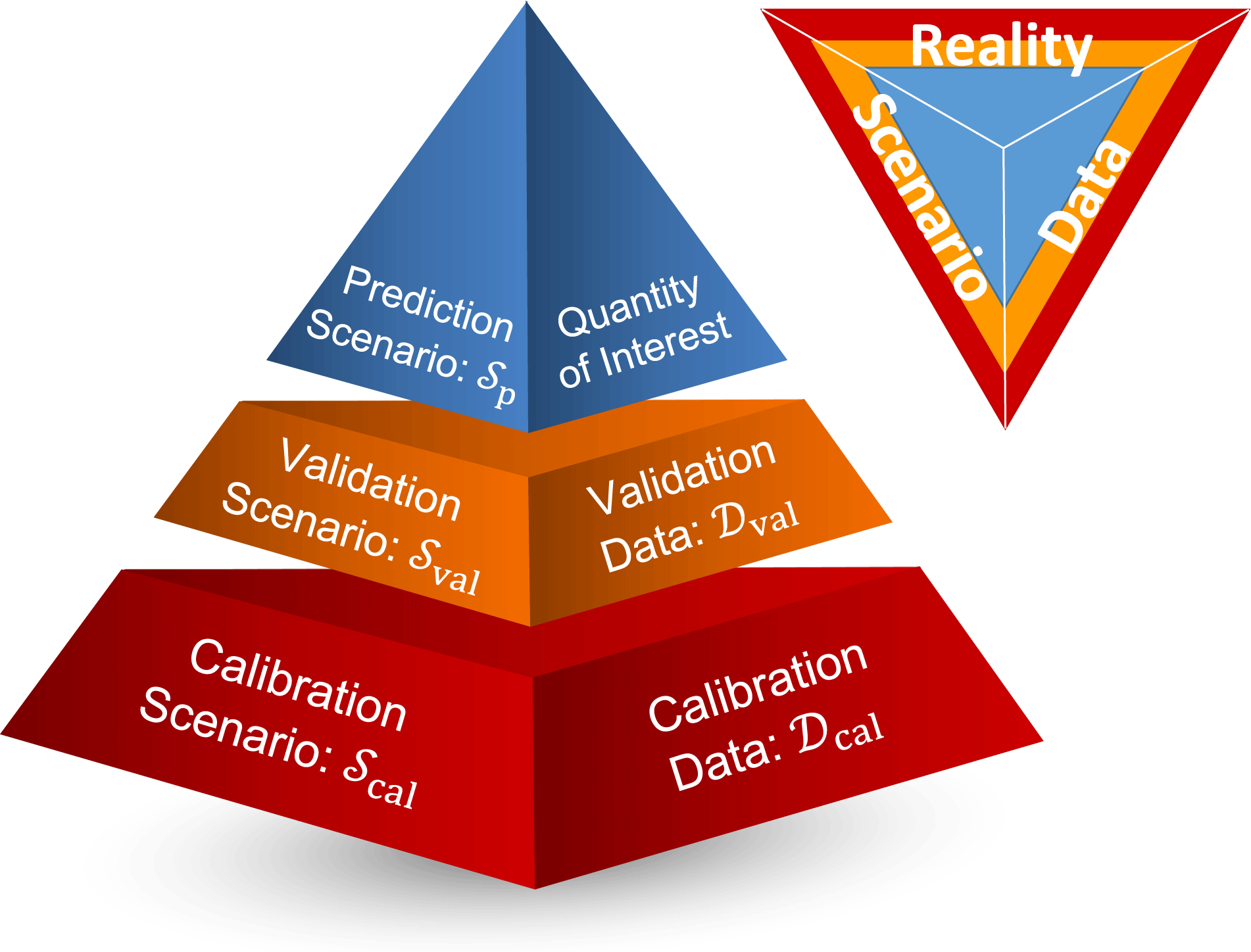
The notion of a scenario is intended to describe the features of the mathematical problem which can be exactly specified, independent of parameters, such as the domain of the solution and certain boundary and initial conditions, the idea being that the same model may be used in several different scenarios. We use the term scenario interchangeably to refer to both the domains in which the mathematical model (2.1) is solved and the actual physical environments in which experimental data are collected, or in which the target quantities to be predicted reside. Later we will argue that it makes sense to consider a hierarchy of scenarios, beginning with component or unit calibration tests in scenarios $S_{c}$ to initially adjust model parameters, then moving to more complex subsystem validation scenarios $S_{v}$ to test the accuracy with which the model can predict observables (to see if the model is ‘valid’), and then the prediction scenario $S_{p}$ , involving the full physical system and model, in which the forward problem (2.1) is solved to predict the quantities of interest (QoIs). A revealing example of various scenarios emerges in models of biomedical systems in which in vitro data are selected in laboratory experiments (e.g. cell proliferation in a Petri dish supplied with concentration of nutrients, or in vitro experiments with laboratory animals) and the models are there expected to be validated using in vivo data collected through biopsies or emerging imaging techniques. These are the calibration scenarios $S_{c}$ (the in vitro experiments) and the validation scenarios $S_{v}$ (the in vivo experiments). The model may then be called upon to make an out-of-data prediction in the prediction scenario $S_{p}$ . We discuss these ideas in more detail later.

To develop a framework for addressing uncertainties, we accept the idea that the model parameters $\boldsymbol{\unicode[STIX]{x1D703}}$ may generally be random vectors. Thus, the solutions $u(\boldsymbol{\unicode[STIX]{x1D703}},S)$ are random or stochastic functions. Problem (2.1), therefore, describes an infinite class of models parametrized by $\boldsymbol{\unicode[STIX]{x1D703}}$ . The mathematical problem characterized by (2.1) is called the forward problem. It describes a projection of data ‘forward’ into a prediction $u(\boldsymbol{\unicode[STIX]{x1D703}},S)$ . Thus, $u(\boldsymbol{\unicode[STIX]{x1D703}},S)$ is the solution of the forward problem. Given observational data, and a mathematical model, the problem of determining the model parameters that best fit the data, in some statistical sense, is the (Bayesian) inverse problems, which we take up in Part 2.

Two basic issues arise at this point.

1. (i) Solutions $u(\boldsymbol{\unicode[STIX]{x1D703}},S)$ to the forward problem must exist for every $\boldsymbol{\unicode[STIX]{x1D703}}\in \unicode[STIX]{x0398}$ . This often-ignored fact leads to conditions on the space $\unicode[STIX]{x0398}$ of parameters. Generally, the solution will be a member of an appropriate space $U$ of random functions.

2. (ii) The fundamental goal of constructing and solving the model (2.1) is not only to determine the solution of the forward problem, but to use these solutions to compute specific QoIs, generally described as functionals $Q$ on the space $U$ containing the solution. This calculation is made in the full prediction scenario, $S=S_{p}$ . Thus, $S_{p}$ pertains to the full system in which the model extrapolates all relevant information to predict an outcome beyond those events available through the analysis of observational data:

   (2.2) $$\begin{eqnarray}Q:U\rightarrow \mathbb{R}:Q(u(\boldsymbol{\unicode[STIX]{x1D703}},S_{p}))=\bar{Q}(\boldsymbol{\unicode[STIX]{x1D703}}).\end{eqnarray}$$
   Clearly, $\bar{Q}$ is, in general, a random function.

The determination of the validity of the model (2.1) as a means of predicting $\bar{Q}$ of (2.2) must, by definition, involve determining the accuracy with which model predictions agree with experimental data – the observations. These data are collected in a model validation scenario $S_{v}$ , which is characterized by an experimental set-up designed to, hopefully, represent how well the model can predict the QoI. As noted earlier, at a lower unit-test level, initial characterizations of model parameters are done in calibration scenario $S_{c}$ , wherein experimental data are used to adjust parameters so as to make model predictions agree with experimental measurements. The full calibration–validation–prediction process is symbolized in a ‘prediction pyramid’ described later (see Figure 5.1).

2.2 Sources of uncertainty in predictions

So what is the anatomy of scientific prediction within the context laid down thus far, and how do we cope with the multitude of uncertainties in each step of the prediction process? We wish to predict a specific reality in a possibly very complex scenario $S_{p}$ using a computational model which is based on a mathematical model of a real situation from which the target QoI can be specified. We must therefore select a model that we hope can deliver a sufficiently accurate estimate of the QoI and for which we have some confidence in its predictability. The predictability of our model rests on knowledge gained through observation – and our access to observational data – and our inductive reasoning embodied in our construction of a model. The model, in general, will be characterized by a set of parameters which themselves are generally unknown, and which at best involve uncertainties. Then we must discretize the mathematical model to produce a computational model, a corruption necessary to render the model into a form that can be processed by digital computers.

Collecting all these sources of uncertainty, and following, in part, the classification plan of Terenin and Draper (Reference Terenin and Draper2015), we list the following sources of uncertainty in predictive computational science and in making prediction of realities.

(5) $h$  uncertainty.

This is uncertainty brought about by the discretization process that produces the computational model – ‘ $h$ ’ representing an appropriate discretization parameter. This uncertainty can sometimes be estimated a posteriori through error estimation or bounded through a priori estimates or at least studied in some quantitative sense through various verification processes.

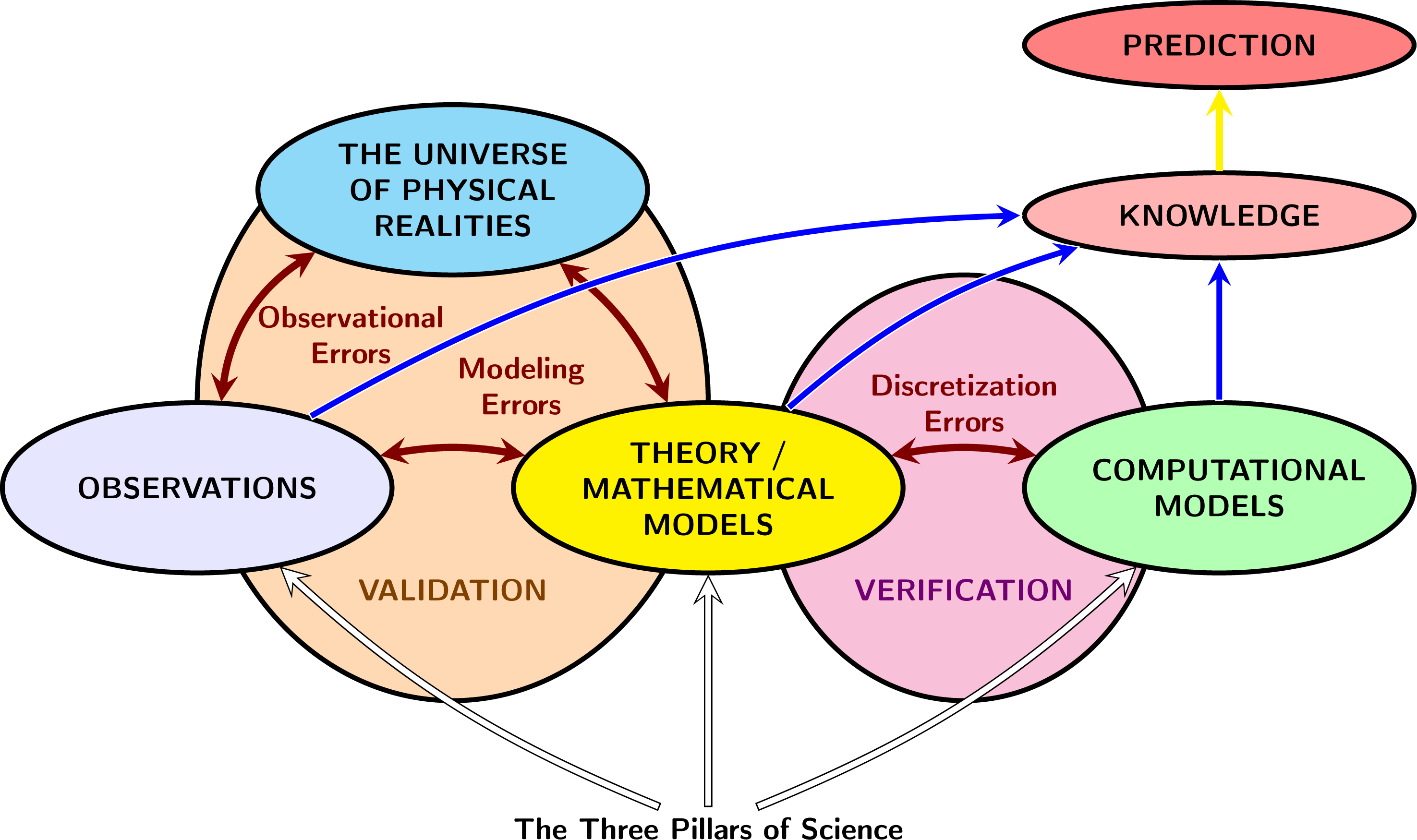
The various paths to knowledge, made imperfect by the uncertainties discussed, are represented symbolically in Figure 2.1.

Figure 2.1.

The imperfect paths to knowledge and prediction. A schematic of the imperfect paths to knowledge that involve uncertainties in all phases of the process for gaining knowledge and making predictions. (From Oden et al. Reference Oden, Moser and Ghattas2010.)

To lay the philosophical foundations for our view of systemic ( ${\mathcal{P}}$ ) uncertainty, we provide a review of the logical theory of probability of Cox and Jaynes, which points to a Bayesian framework for studying most of the sources of uncertainty. Then we review briefly the Fisher/frequentist approach to problems in statistical analysis.

3.1 Plausible reasoning

The notion of logical or Cox–Jaynes probability begins with the concept of plausible reasoning. The idea is that in science, and indeed, in everyday life, we rarely have enough information to permit deductive reasoning. Instead, we make plausible conclusions based on past experience. Certain reasoning processes assess the plausibility of a proposition accepting that it may not be a certainty. Thus, we regard the logical approach to scientific reasoning as one way of assessing the plausibility of a proposition (as opposed to the frequency of an event) that can be true or false or that can be assigned a degree of plausibility.

The appropriate mathematical setting for such considerations is that furnished by a Boolean algebra.

Propositional Boolean algebra. A propositional Boolean algebra $C$ consists of the 6-tuple

(3.1) $$\begin{eqnarray}C\sim \{{\mathcal{A}},\wedge ,\vee ,\neg ,\mathbf{0},\mathbf{1}\},\end{eqnarray}$$

wherein

• ∙ ${\mathcal{A}}=$ a set of true propositions, which might be finite, countable or uncountable;

• ∙ two binary operations, $\wedge$ and $\vee$ , and a unitary operation $\neg$ on the propositions in ${\mathcal{A}}$ , i.e.,

  1. – $A\wedge B=$ the conjunction of $A$ and $B$ , meaning that both $A$ and $B$ are true,

  2. – $A\vee B=$ the disjunction of $A$ and $B$ , meaning that at least one of $A$ and $B$ is true (‘ $A$ or $B$ ’),

  3. – $\neg A=A\neg =$ the negation of $A$ , meaning $A$ is false;

• ∙ two identity elements $\mathbf{0}$ and $\mathbf{1}$ .

We also require the following.

1. (i) $C$ is closed under countable applications of $\wedge$ and $\vee$ .

2. (ii) For all propositions $(A,B,C)\in {\mathcal{A}}$ , the following five Boolean axioms hold.

   Associative laws:

   $$\begin{eqnarray}A\wedge (B\wedge C)=(A\wedge B)\wedge C,\quad A\vee (B\vee C)=(A\vee B)\vee C.\end{eqnarray}$$

   Commutative laws:

   $$\begin{eqnarray}A\wedge B=B\wedge A,\quad A\vee B=B\vee A.\end{eqnarray}$$

   Identity elements:

   $$\begin{eqnarray}A\wedge \mathbf{1}=A,\quad A\vee \mathbf{0}=A.\end{eqnarray}$$

   Complementation or negation:

   $$\begin{eqnarray}A\wedge (\neg A)=\mathbf{0},\quad A\vee (\neg A)=\mathbf{1}.\end{eqnarray}$$

   Distributive laws:

   $$\begin{eqnarray}\displaystyle A\wedge (B\vee C) & = & \displaystyle (A\wedge B)\vee (A\wedge C),\nonumber\\ \displaystyle A\vee (B\wedge C) & = & \displaystyle (A\vee B)\wedge (A\vee C).\nonumber\end{eqnarray}$$

The conjunction of two propositions $A\wedge B$ is also written $AB$ , i.e. as a ‘product’, and the disjunction $A\vee B$ is written as the sum $A+B$ , all in analogy with the (‘two-valued’) algebra of numbers. In this context, the Boolean algebra of propositions is said to follow the rules of Aristotelian logic.

The plausibility of a proposition $A$ , given that a proposition $B$ is true, is characterized by a real-valued function $pl(.|.)$ on pairs of propositions:

(3.2) $$\begin{eqnarray}pl:{\mathcal{A}}\times {\mathcal{A}}/\mathbf{0}\quad \rightarrow \mathbb{R}^{+}.\end{eqnarray}$$

Thus $pl(A|B)$ is the degree of plausibility of proposition $A$ given that $B$ is true. If $B$ is true, $A$ becomes plausible, while evidence does not guarantee that $A$ is true, but by observation of one or more of its consequences gives confidence that $A$ is plausible. Also, if, given $B$ , $A$ is more plausible than $C$ , we have $pl(A|B)>pl(C|B)$ . Other fundamental rules will follow.

Jaynes’ example (Jaynes Reference Jaynes2003). Suppose we state the proposition $A\sim$ ‘it will start raining at 10.00 a.m. at the latest’, and $B\sim$ ‘the sky will become cloudy before 10.00 a.m.’ Plausible reasoning not only establishes whether a proposition is more or less plausible, it evaluates the degree of plausibility in some way. For example the darkness of the clouds may suggest the degree of plausibility of rain.

3.2 Logic and philosophical theories of probability

Logic is the science of reasoning, an intellectual discipline with origins dating back millennia, that provides the cornerstones to mathematics, science and all forms of human knowledge.

As noted in Section 2, deductive logic or logical deduction is a form of reasoning from one or more premises or axioms so as to deduce a logically certain conclusion. Deductive logic is infallible and irrevocable when its conclusions are reached by following strict laws of reasoning. Mathematics is a discipline founded on deductive logic: one lays down axioms and definitions and then deduces their consequences following rules of logic. According to Jaynes (Reference Jaynes2003), however, all knowledge is inductive. In deductive reasoning, if $A$ and $B$ are elements or propositions, one writes $A\Rightarrow B$ to mean if $A$ is true, $B$ is logically deduced from $A$ . According to Jaynes (Reference Jaynes2003, p. 4), in almost all situations, ‘we do not have the right kind of information to allow this kind of reasoning’. In the formal logic of plausible reasoning $A\Rightarrow B$ means only that $A$ and $B$ have the same ‘truth value’.

If $A$ and $B$ are true propositions, a proposition $C$ which is a function $f$ of $A$ and $B$ , ( $C=f(A,B)$ ), can be either true or false. Since $A$ and $B$ take on values $[TT,TF,FT,FF]$ , there are 16 logical functions: $f(T,T)=T,f(T,T)=F,\ldots$ etc. Thus a logical function of $n$ propositions has $2^{n}$ function values. One can therefore construct truth tables analogous to the theory of elementary logic of operations on real numbers, to cover possible truth values of such logic functions.

Plausible reasoning not only establishes whether a proposition is more or less plausible, it evaluates the degree of plausibility in some way (e.g. the darkness of the clouds may suggest the plausibility of rain). Examples of the Boolean algebra of propositions are as follows.

• ∙ $A,B,C,\ldots =$ propositions = unambiguous, simple, definitive, statements that are either true or false (two-valued Aristotelian logic)

• ∙ As noted earlier, conjunction ‘cojoins’ two propositions into a ‘logical product’:

  $$\begin{eqnarray}A\wedge B=AB\quad (\text{both }A\text{ and }B\text{ are true}).\end{eqnarray}$$

• ∙ Disjunction, called the ‘logical sum’, ‘disjoins’ two propositions:

  $$\begin{eqnarray}A\vee B=A+B\quad (\text{at least one of }A\text{ and }B\text{ are true}).\end{eqnarray}$$

• ∙ Negation describes ‘denial’:

  $$\begin{eqnarray}\neg A\equiv A\quad \text{is false}.\end{eqnarray}$$

• ∙ We understand equality and identity of propositions as

  $$\begin{eqnarray}\displaystyle A & = & \displaystyle B\quad (A\text{ and }B\text{ are equal in truth (or `truth value')}),\nonumber\\ \displaystyle A & \equiv & \displaystyle B\quad (A\text{ and }B\text{ are equal by definition}).\nonumber\end{eqnarray}$$

Some properties:

• ∙ $A\vee \neg A=$ a necessary (or logical) truth ( $A$ is either true or false),

• ∙ $A\wedge \neg A=$ a necessary (or logical) falsehood ( $A$ is true and false),

• ∙ $\neg A\wedge B=AB$ is false,

• ∙ $\neg A\wedge \neg B=$ both $A$ and $B$ are false,

• ∙ if $C=A\wedge B$ , then $\neg C=\neg A\vee \neg B$ ,

• ∙ if $D=A\vee B$ , then $\neg D=\neg A\wedge \neg B$ .

These properties are recognized as analogous to elementary set properties with $A,B,C,D$ sets, $AB=A\cup B$ , $A+B=A\cap B$ , $\bar{A}=A^{\prime }$ , etc.  $A\Rightarrow B$ ( $A$ implies $B$ ) does not assert that either $A$ or $B$ is true, it means $A\wedge \bar{B}$ ( $A$ and ( $B$ is false)) is false or $\bar{A}\vee B$ (either $A$ is false or $B$ is true) is true.

3.3 Van Horn’s guide to Cox’s theorem

It is informative to follow a few arguments given by Van Horn in his guide to Cox’s theorem (Van Horn Reference Van Horn2003). There are two central notions.

1. (i) The state of information $X$ summarizes the information one has on what is called the ‘atomic proposition $\unicode[STIX]{x1D6EC}$ ’: those that cannot be decomposed into other propositions. These atomic propositions form the basis for the state of information $X$ .

2. (ii) The plausibility of a proposition $A\in {\mathcal{A}}$ , given the state of information $X$ , is a number $pl(A|X)$ : the state of information obtained from $A$ by adding the additional information that $X$ is true, thus written $(AX)$ or $(A|X)$ .

We may now lay down several assumptions. In the notation inspired by Van Horn, there are five ‘rules’, $\text{R1},\ldots ,\text{R5}$ .

R5.

Given $S(T)$ and a tautology $T$ , there exists a continuous function $F:[S(T),T]^{2}\rightarrow [S(T),T]$ , strictly increasing on $(S(T),T]$ , such that

(3.3) $$\begin{eqnarray}pl(A\wedge B|X)=F[pl(A|B,X),pl(B|X)]\end{eqnarray}$$

for any $A$ , $B$ and consistent $X$ .

The establishment of (3.3) follows some surprisingly intuitive arguments. We begin by writing down all the combinations of $A$ , $B$ and $X$ that $pl(A\wedge B|X)$ could be a function of (omitting ‘ $pl$ ’ temporarily, for simplicity), they are $(A|X)$ , $(B|X)$ , $(A|B,X)$ and $(B|A,X)$ and all combinations of these numbers, 15 in all. Because $A\wedge B=B\wedge A$ , only nine of these survive. Van Horn (Reference Van Horn2003), following Tribus (Reference Tribus2016), rules out as many of these as possible:

1. (1) $(A\wedge B|X)=F[(A|X)]$ ,

2. (2) $(A\wedge B|X)=F[(A|BX)]$ ,

3. (3) $(A\wedge B|X)=F[(A|X),(A|BX)]$ ,

4. (4) $(A\wedge B|X)=F[(A|BX),(B|AX)]$ ,

5. (5) $(A\wedge B|X)=F[(A|X),(B|X)]$ .

Remarkably, all five of these candidates lead to a contradiction and can, therefore, be discarded. For example, in (1), if $A$ is a tautology (a fundamental truth) and $B$ is a ‘atomic’ proposition, then $A\wedge B$ is equivalent to $B$ and $(A|X)=T$ , so $S(T)=(B|X)$ . But $X$ can always be chosen to make $(B|X)$ any value in $Y_{\circ }$ . So we have a contradiction. Therefore (1) cannot hold. Similarly, in (3), for instance, if $A$ is a tautology and $B$ is any atomic proposition, then $S(T)=(B|X)$ , a contradiction. Similar arguments can be made for all these candidates leaving only four possibilities out of the original 15:

1. (I) $(A\wedge B|X)=F[(A|BX),(B|X)]$ ,

2. (II) $(A\wedge B|X)=F[(A|B,X),(B|X),(A|X)]$ ,

3. (III) $(A\wedge B|X)=F[(A|B,X),(B|X),(B|A,X)]$ ,

4. (IV) $(A\wedge B|X)=F[(A|B,X),(B|X),(B|A,X),(A|X)]$ .

Van Horn refers to the arguments of Tribus (Reference Tribus2016) who claims that (III) and (IV) can be ruled out because ‘one cannot avoid dealing with plausibility expressions that involve some inconsistent state of information $Y$ , and hence there is unavoidable ambiguity’ (Van Horn Reference Van Horn2003, p. 16). Also, rule (II) is eliminated for certain similar reasons, leaving only (I). But Van Horn asserts that ‘there is no completely compelling reason for choosing any particular one of the four remaining candidates’. He leans toward (I) as the other candidates merely add additional conditions to those used in (I) and because Jaynes (Reference Jaynes2003) provides an intuitive argument in support of (I).

Assuming (I) holds, next consider the plausibility $A\wedge B\wedge C|X$ ), $X$ being consistent. Applying rule (I), with ‘ $B$ ’ now replaced by $(B\wedge C)$ , gives

(3.4) $$\begin{eqnarray}\displaystyle (A\wedge (B\wedge C)|X) & = & \displaystyle F[(A|(B\wedge C),X),((B\wedge C)|X)]\nonumber\\ \displaystyle & = & \displaystyle F[(A|B,C,X),F[(B|C),X),(C|X)]].\end{eqnarray}$$

Now use the equivalent grouping of the propositions on the left-hand side:

(3.5) $$\begin{eqnarray}\displaystyle ((A\wedge B)\wedge C|X) & = & \displaystyle F[((A\wedge B)|C,X),(C|X)]\nonumber\\ \displaystyle & = & \displaystyle F[F[(A|B,CX),(B|C,X)](C|X)].\end{eqnarray}$$

But $A\wedge (B\wedge C)=(A\wedge B)\wedge C$ , so the functions derived in (3.4) and (3.5) must coincide. Setting

$$\begin{eqnarray}\displaystyle x & = & \displaystyle (A|B,C,X),\nonumber\\ \displaystyle y & = & \displaystyle (B|C,X),\quad \text{and}\nonumber\\ \displaystyle z & = & \displaystyle (C|X),\nonumber\end{eqnarray}$$

where $x,y,z\in [0,T]$ , we are looking for a function $F$ that for numbers $x,y,z$ is such that

(3.6) $$\begin{eqnarray}F(x,F(y,z))=F(F(x,y),z).\end{eqnarray}$$

Since $F$ is continuous and dense, this relation holds for all $x,y,z\in [0,T]$ . This property of denseness is fundamental to Cox’s theorem. The fact that ‘ $\wedge$ ’ is associative ensures that $F$ is associative, which limits choices for $F$ to be ‘isomorphic to multiplication’. A little inventory: if we can find any function $F$ satisfying (3.6), then, by rule (I), we will have determined how the ‘product’ $A\wedge B$ , conditional on $X$ , depends on $(A|BX)$ and $(B|X)$ . Thus, we establish (3.3).

Equation (3.6) is called the associativity equation; it is an example of a functional equation. Such equations are studied in Aczel (Reference Aczel1966), where the following theorem can be found.

Theorem 3.1 (Aczel’s theorem).

Let $f:(a,b]^{2}\rightarrow (a,b]$ be a continuous, strictly increasing function in both arguments $a$ and $b$ , with $a,b\in \mathbb{R}$ and $a<b$ , and suppose that for all $x,y,z\in (a,b]$ ,

$$\begin{eqnarray}f(x,f(y,z))=f(f(x,y),z).\end{eqnarray}$$

Then there exist a continuous, strictly increasing function $g$ such that

$$\begin{eqnarray}g(f(x,y))=g(x)+g(y)\end{eqnarray}$$

for all $x,y\in (a,b]$ .

Now set $f=F$ , $a=S(T)$ , $b=T$ and define a real-valued, continuous, increasing, and non-negative function $w=w(x)$ on $(S(T),T]$ such that

$$\begin{eqnarray}\ln w(x)=g(x),\quad x\in [S(T),T].\end{eqnarray}$$

with $w(S(T))$ the limit as $x\rightarrow S(T)$ . We then must have by continuity

$$\begin{eqnarray}w(F(x,y))=w(x)w(y),\end{eqnarray}$$

for $x,y\in [S(T),T]$ . Thus, for every $A,B\in {\mathcal{A}}$ and consistent $X$ , we have

(3.7) $$\begin{eqnarray}w((A\wedge B|X))=w((A|B,X))w((B|X)).\end{eqnarray}$$

The function $w$ thus suggests that conditional probabilities obey a ‘product rule’ similar to probabilities (e.g.  $\mathbb{P}(A\cup B)=\mathbb{P}(A|B)\mathbb{P}(B)$ , now conditioned on information $X$ ).

A final step for the product rule calls upon the fact that

$$\begin{eqnarray}w(S(T))=0,\quad w(T)=1,\quad \text{and }~0<w(x)<1\quad \text{for }S(T)<x<T.\end{eqnarray}$$

A proof of this assertion is given in Van Horn (Reference Van Horn2003). Briefly, it involves the observation that for any proposition $A$ , consistent $X$ and tautology  $D$ ,

$$\begin{eqnarray}w((A|X))=w((D\wedge A|X))=w((D|A,X))w((A|X))=w(T)w((A|X)),\end{eqnarray}$$

so dividing by $w((A|X))$ gives $w(T)=1$ and, therefore, $w(x)<1$ for $x<T$ . The proof that $w(S(T))=0$ follows from contradiction: assume otherwise and consider $A_{1},A_{2}\in {\mathcal{A}}$ and $x\in Y_{\circ }$ . If $w(S(T))=y>0$ , then $0<z<1$ and $z<\sqrt{z}<1$ , $w^{-1}(z)<x<w^{-1}(\sqrt{z})$ . If $(A_{1}|X)=(A_{1},A_{2}|X)=x$ , then $w((A_{1}\wedge A_{2}|X))=w^{2}(x)<z=w(S(T))$ , so $(A_{1}\wedge A_{2}|X)<S(T)$ , a contradiction.

So we can add to (3.7) the condition that the monotone continuous function satisfying (3.7) must also satisfy

(3.8) $$\begin{eqnarray}0\leq w(x)\leq 1,\end{eqnarray}$$

with $w(x)=0$ when $x$ is impossible and $w(x)=1$ when $x$ is certain.

Disjunction (the sum rule for plausibilities).

The aim of the sum or disjunction rule for plausibilities defined on pairs of propositions is to establish a relationship involving the plausibility of a proposition $A$ conditioned on consistent $X$ and its negation $\neg A$ conditioned on $X$ . Full details can be found in Van Horn (Reference Van Horn2003) and Paris (Reference Paris1994). It suffices here to point out that a thread of logic similar to that in the conjunction relations leads again to a functional equation of the form

(3.9) $$\begin{eqnarray}yS\biggl(\displaystyle \frac{x}{y}\biggr)=S(x)S(S(y)/S(x))\end{eqnarray}$$

for all $0<x\leq y<1$ , where

$$\begin{eqnarray}\displaystyle yS\biggl(\displaystyle \frac{x}{y}\biggr) & = & \displaystyle p(\neg A\wedge B|X),\nonumber\\ \displaystyle S(y) & = & \displaystyle p((A\vee \neg B)\wedge (\neg A\vee \neg B)|X),\nonumber\\ \displaystyle S(x) & = & \displaystyle p(\neg A\vee \neg B|X),\nonumber\end{eqnarray}$$

$p(x)=w(x)^{m}$ , $m=-\log (2)/\log w(\unicode[STIX]{x1D6FC})$ , and $\unicode[STIX]{x1D6FC}$ is a fixed point of a map such that $S(A|X)=(\neg A|X)$ for all $A$ and consistent $X$ . From these relations, it possible to show that

(3.10) $$\begin{eqnarray}w^{m}(\neg A|X)+w^{m}(A|X)=1,\end{eqnarray}$$

for positive $m$ . This is known as the sum rule. We note that the product rule (3.7) can be equally well be written as

$$\begin{eqnarray}w^{m}((A\wedge B|X))=w^{m}((A|BX))w^{m}((B|X)),\end{eqnarray}$$

for positive $m$ . For whatever $m$ we choose, we can set

$$\begin{eqnarray}pl(x)=w^{m}(x).\end{eqnarray}$$

Collecting all of the results laid down thus far, we arrive at the following version of Cox’s theorem.

Theorem 3.2 (Cox’s theorem via Van Horn).

Given that rules R1–R5 hold, there exists a continuous, strictly increasing function $pl:{\mathcal{A}}\times {\mathcal{A}}\backslash \mathbf{0}\rightarrow \mathbb{R}^{+}$ such that for every $A$ and $B\in {\mathcal{A}}$ and consistent $X$ :

1. (i) $pl(A|X)=0$ if and only if $A$ is known to be false, given the information  $X$ ;

2. (ii) $pl(A|X)=1$ if and only if $A$ is known to be true given the information  $X$ ;

3. (iii) $0\leq pl(A|X)\leq 1$ ;

4. (iv) $pl(A\wedge B|X)=pl(A|X)~pl(B|A,X)$ ;

5. (v) $pl(\neg A|X)=1-pl(A|X)$ .

Because of the commutative property, $A\wedge B=B\wedge A$ , assertion (iv) in Cox’s theorem implies that

(3.11) $$\begin{eqnarray}pl(A|X)pl(B|AX)=pl(B|X)pl(A|BX),\end{eqnarray}$$

which is recognized as Bayes’ rule, provided we interpret the plausibilities as probabilities.

The five properties laid dawn in Cox’s theorem are formally the rules of probability theory, stated in terms of plausibilities. As pointed out by Van Horn (Reference Van Horn2003, pp. 21–22), ‘any system of plausible reasoning that is not isomorphic to probability theory must necessarily violate one of the requirements’ (in the theorem). So ‘set-theoretical probability theory then becomes the model theory for our logic’. We may thus interpret states of information to be probability distributions, with $AX$ understood to be ‘the probability distribution obtained from $X$ by conditioning the set of values for which $A$ is true’. Henceforth, we refer to the Cox–Jaynes plausibilities as probabilities in the spirit of those covered in the previous section.

Property (iv) sets the Cox–Jaynes theory apart, in a sense, from frequentist theory, featuring conditional probability and Bayes’ rule as a central property of the theory. The existence of the Kolmogorov set-theoretic framework of probability, which involves the same rules, proves that these rules are not contradictory, the primary difference being that in Cox theory, conditional probability is now the fundamental measure. In the Kolmogorov theory described earlier, all probabilities are conditioned on the choice of the sample set $\unicode[STIX]{x03A9}$ .

3.4 The Terenin–Draper account of Cox’s theorem and Cox–Jaynes probability

Terenin and Draper (Reference Terenin and Draper2015) provide a detailed account of the structure and different philosophical issues underlying major probability theories, particularly Kolmogorov’s set-theoretic theory based on the frequentist definition of probability and the Cox–Jaynes theory based on the notions of plausible reasoning. Some key aspects of their arguments are summarized in the following paragraphs.

3.5 Summary comments

Among conclusions that can be drawn from the developments outlined in this section are the following.

• ∙ The Cox–Jaynes theory of logical probability, based on the notions of plausible reasoning and on plausibilities defined on propositional Boolean algebras, is a self-consistent theory, equivalent to the Kolmogorov theory, but structured in a framework in which conditional probability is the primitive concept. In this sense, there is no ${\mathcal{P}}$  uncertainty if this theory of probability is employed to deal with uncertainties.

• ∙ The natural extension of Aristotelian logic with uncertainties is Bayesian (see Jaynes Reference Jaynes2003).

We are thus on solid ground to study the major components of predictive science – at least many of them – within a Bayesian framework.

4.1 Bayes’ rule for parametric models

Recall that in Section 2.2 we considered the predictability of models defining a forward problem with a solution $u=u(\boldsymbol{\unicode[STIX]{x1D703}},S)$ depending on parameters $\boldsymbol{\unicode[STIX]{x1D703}}\in \unicode[STIX]{x0398}$ and set in a scenario $S$ for a problem ${\mathcal{A}}(\boldsymbol{\unicode[STIX]{x1D703}},S;u(\boldsymbol{\unicode[STIX]{x1D703}},\boldsymbol{S}))=0$ , and we considered the question of predictability of such models in the presence of uncertainty, addressing the principal sources of uncertainty described: ${\mathcal{P}}$ , ${\mathcal{M}}$ , ${\mathcal{Y}}$ , $\boldsymbol{\unicode[STIX]{x1D703}}$ and $h$  uncertainty. We will now explore these uncertainties in a Bayesian formalism.

As noted in Sections 3.3 and 3.4, we can dispense with ${\mathcal{P}}$ uncertainty immediately. We argued that within the framework of Cox–Jaynes probability theory (and equivalently, Kolmogorov theory), there is no ${\mathcal{P}}$  uncertainty, and every natural extension of Aristotelian logic in the presence of uncertainties is Bayesian Terenin and Draper (Reference Terenin and Draper2015). We will therefore employ tools and also concepts from the equivalent Kolmogorov theory when convenient. This leaves us with ${\mathcal{M}}$ , ${\mathcal{Y}}$ , $\boldsymbol{\unicode[STIX]{x1D703}}$ and $h$  uncertainties.

Terenin and Draper (Reference Terenin and Draper2015, p. 18) state that ‘All uncertainty in probabilistic models is therefore the result of model specification: either via the parameters ( $\unicode[STIX]{x1D703}$ -uncertainty), or via the structure of the model itself ( ${\mathcal{M}}$ -uncertainty).’ We add to this uncertainty in the data ( ${\mathcal{Y}}$  uncertainty) and, since we are interested in computational models obtained through discretization of mathematical models, $h$  uncertainty as well.

This latter area, $h$  uncertainties, is in the realm of model verification and is either an issue of code verification, requiring such things as documentation, version control, benchmarks, etc., or solution verification, which is a matter of mathematically based a posteriori error estimation.

We will ignore $h$ uncertainty in this article as it is dealt with in detail in other accounts (e.g. Ainsworth and Oden Reference Ainsworth and Oden2000). That leaves us with ${\mathcal{M}}$ , ${\mathcal{Y}}$ and $\boldsymbol{\unicode[STIX]{x1D703}}$ uncertainties. ${\mathcal{M}}$  uncertainty is a deep and challenging subject involving the study of model selection, model inadequacy, and the complicated interaction of uncertainties in the model with those in data and parameters. We take up this important subject after first looking at ${\mathcal{Y}}$ and $\boldsymbol{\unicode[STIX]{x1D703}}$ uncertainty in Section 8. First, we address ${\mathcal{Y}}$ and $\boldsymbol{\unicode[STIX]{x1D703}}$ , beginning with their appearance in Bayes’ rule, where one finds naturally the push and pull of the two classical pillars of science: observation, with uncertain data $\boldsymbol{y}\in Y$ , and theory, represented by unvalidated models with uncertain parameters $\boldsymbol{\unicode[STIX]{x1D703}}\in \unicode[STIX]{x0398}$ .

Thus, from Bayes’ rule, we covert to probability densities $\unicode[STIX]{x1D70B}$ , and from the rule $\mathbb{P}(A|B)=\mathbb{P}(B|A)\mathbb{P}(A)/\mathbb{P}(B)$ , we let $B$ represent the observational data $\boldsymbol{y}$ for scenario $S$ and $A$ represent the model parameters $\boldsymbol{\unicode[STIX]{x1D703}}$ , leading to

(4.1) $$\begin{eqnarray}\unicode[STIX]{x1D70B}(\boldsymbol{\unicode[STIX]{x1D703}}|\boldsymbol{y},S)=\displaystyle \frac{\unicode[STIX]{x1D70B}(\boldsymbol{y}|\boldsymbol{\unicode[STIX]{x1D703}},S)\unicode[STIX]{x1D70B}(\boldsymbol{\unicode[STIX]{x1D703}}|S)}{\unicode[STIX]{x1D70B}(\boldsymbol{y}|S)},\end{eqnarray}$$

where $\unicode[STIX]{x1D70B}(\boldsymbol{\unicode[STIX]{x1D703}}|S)$ is the prior density of parameters $\boldsymbol{\unicode[STIX]{x1D703}}\in \unicode[STIX]{x0398}$ for scenario $S$ , $\unicode[STIX]{x1D70B}(\boldsymbol{y}|\boldsymbol{\unicode[STIX]{x1D703}},S)$ is the likelihood, $\unicode[STIX]{x1D70B}(\boldsymbol{\unicode[STIX]{x1D703}}|\boldsymbol{y},S)$ is the posterior density, and $\unicode[STIX]{x1D70B}(\boldsymbol{y}|S)$ is the evidence. Since $\int _{\unicode[STIX]{x0398}}\unicode[STIX]{x1D70B}(\boldsymbol{\unicode[STIX]{x1D703}}|\boldsymbol{y},S)\text{d}\boldsymbol{\unicode[STIX]{x1D703}}=1$ for all $\boldsymbol{y}$ in the space ${\mathcal{Y}}$ of observational data and for all scenarios $S$ ( $S_{c}$ , the calibration scenarios; $S_{v}$ , the validation scenarios; $S_{p}$ , the prediction scenario), the evidence must be the marginalization of the numerator,

(4.2) $$\begin{eqnarray}\unicode[STIX]{x1D70B}(\boldsymbol{y}|S)=\int _{\unicode[STIX]{x0398}}\unicode[STIX]{x1D70B}(\boldsymbol{y}|\boldsymbol{\unicode[STIX]{x1D703}},S)\unicode[STIX]{x1D70B}(\boldsymbol{\unicode[STIX]{x1D703}}|S)\text{d}\boldsymbol{\unicode[STIX]{x1D703}}.\end{eqnarray}$$

Here $\boldsymbol{y}=(\boldsymbol{y}_{1},\boldsymbol{y}_{2},\ldots ,\boldsymbol{y}_{n})\in {\mathcal{Y}}_{s}\subset \mathbb{R}^{n}$ , and it is understood that (4.2) holds for every scenario $S$ , the data $\boldsymbol{y}$ being different in each.

4.2 Data uncertainty: experimental noise

Bayes’ rule (4.1) embraces all of the pillars of science drawn upon to acquire (or increase) one’s knowledge: observations, characterized by observational data $\boldsymbol{y}\in {\mathcal{Y}}$ , theory, the mathematical modelling of hypotheses founded on inductive logic, put forth to explain observed events, and computations, needed to evaluate the resulting distributions. To the classical statistician, models are represented by the likelihood $\unicode[STIX]{x1D70B}(\boldsymbol{y}|\boldsymbol{\unicode[STIX]{x1D703}},S)$ , $\boldsymbol{\unicode[STIX]{x1D703}}$ representing specific features of the model and $\unicode[STIX]{x1D70B}(\boldsymbol{y}|\boldsymbol{\unicode[STIX]{x1D703}},S)$ the probability distribution for data given $\boldsymbol{\unicode[STIX]{x1D703}}$ , for any scenario $S$ ; the outcome, $\unicode[STIX]{x1D70B}(\boldsymbol{\unicode[STIX]{x1D703}}|\boldsymbol{y},S)$ , is the result of the information in the data and the predictability of the model. To the scientist or engineer, this statistical model is reached after a process of using the solution of the forward problem to evaluate the observations available to the models. These predictions of $\boldsymbol{y}$ of the models are quantities $\boldsymbol{d}(\boldsymbol{\unicode[STIX]{x1D703}},S)$ which rarely coincide with the recorded observations $\boldsymbol{y}$ .

Let us consider the problem of using model (4.1) for a given scenario $S$ to predict the value of some physical entity. The target prediction could be, for example, the temperature at a point in a turbine engine, the volume fraction of cancer cells in a sample of human tissue, the maximum von Mises stress in a machine part, or the time-to-failure of a steel shaft in an aircraft engine. Such quantities are rarely deterministic. A fundamental assumption in classical mathematical statistics is that the physical entity we wish to predict with model (4.1) in any particular scenario $S$ is determined by a stochastic law (the ‘true’ structure of the entity) characterized by a probability distribution $\boldsymbol{G}$ with density $\boldsymbol{g}$ . The structure of $\boldsymbol{g}$ (or $\boldsymbol{G}$ ) is available to us only through samples taken from a set of experiments, the experimental observations $\boldsymbol{y}$ , which are generally corrupted by experimental noise $\boldsymbol{\unicode[STIX]{x1D716}}$ (or experimental errors), since no measuring device is perfect. The observations $\boldsymbol{y}$ are realizations of a random variable $Y$ .

But the observational data we record is not the truth; rather it is some function $\boldsymbol{f}$ of the true density $\boldsymbol{g}$ and of unknown experimental errors $\boldsymbol{\unicode[STIX]{x1D716}}$ , often called the experimental noise:

(4.3) $$\begin{eqnarray}\boldsymbol{y}=\boldsymbol{f}(\boldsymbol{g},\boldsymbol{\unicode[STIX]{x1D716}})\end{eqnarray}$$

(or the so-called stochastic extension $Y=f(\boldsymbol{G},E)$ ). To go further, we must assume (or construct) an appropriate form of $\boldsymbol{f}$ and propose a probability distribution $p_{noise}(\boldsymbol{\unicode[STIX]{x1D716}})$ for $\boldsymbol{\unicode[STIX]{x1D716}}$ . These constitute a noise model. The construction of an appropriate noise model for observational data is often a challenging endeavour requiring detailed information on the measurement processes and instrumentation. This may often mean we must construct a new parametric model of $\boldsymbol{g}$ , knowing very little about the ‘truth’. But there are approaches, some discussed later in this article, of constructing approximations of $\boldsymbol{g}$ that may improve in accuracy as new data are acquired. These approximations involve new parameters, not the parameters $\boldsymbol{\unicode[STIX]{x1D703}}$ of the model of the forward problem – sometimes called hyperparameters. Methods for estimating these parameters and enhancing our approximation of $\boldsymbol{g}$ are discussed later (e.g. Section 5.3).

In the majority of statistics applications, the most common noise model is the additive model

(4.4) $$\begin{eqnarray}\boldsymbol{g}+\boldsymbol{\unicode[STIX]{x1D716}}=\boldsymbol{y},\end{eqnarray}$$

showing an additive correction to the truth is what is observed; the noise distribution $p_{noise}(\boldsymbol{\unicode[STIX]{x1D716}})$ is often assumed to be Gaussian. The extra parameters in the definition of $p_{noise}(\cdot )$ may be added to the model parameters to produce the total parameter vector $\boldsymbol{\unicode[STIX]{x1D703}}$ . If we have $n$ samples of $\boldsymbol{g}$ , (4.4) is replaced by

(4.5) $$\begin{eqnarray}\boldsymbol{g}_{i}+\boldsymbol{\unicode[STIX]{x1D716}}_{i}=\boldsymbol{y}_{i},\quad 1\leq i\geq n.\end{eqnarray}$$

4.3 Model inadequacy

The experimental noise in general is a result of the methods and devices used to gather observational data and is independent of the model and of model parameters. Now let us consider how well the model predicts realities of various scenarios.

Having solved the forward problem for scenario $S$ , use the solution $u(\boldsymbol{\unicode[STIX]{x1D703}},S)$ to compute the model predictions of reality $\boldsymbol{g}_{i}$ for parameter $\boldsymbol{\unicode[STIX]{x1D703}}$ . We denote such predictions by a parameter-to-observation map $B:U\rightarrow {\mathcal{Y}}$ such that $B_{i}(u(\boldsymbol{\unicode[STIX]{x1D703}},S))=d_{i}(\boldsymbol{\unicode[STIX]{x1D703}},S)$ . Since the model is imperfect, a modelling error $\unicode[STIX]{x1D6FE}_{i}(\boldsymbol{\unicode[STIX]{x1D703}},S)$ occurs, assumed for simplicity to be additive:

(4.6) $$\begin{eqnarray}\boldsymbol{g}_{i}=\boldsymbol{d}_{i}(\boldsymbol{\unicode[STIX]{x1D703}},S)+\unicode[STIX]{x1D738}_{i}(\boldsymbol{\unicode[STIX]{x1D703}},S),\quad 1\leq i\geq n.\end{eqnarray}$$

where $\unicode[STIX]{x1D738}_{i}(\boldsymbol{\unicode[STIX]{x1D703}},S)$ is defined as the model inadequacy, or model form error, or model bias (AIAA 1998, ASME 2006, Oberkampf and Roy Reference Oberkampf and Roy2010, Oden et al. Reference Oden, Babuška, Faghihi, Stein, de Borst and Hughes2018, Kennedy and O’Hagan Reference Kennedy and O’Hagan2001). This can be regarded as a component of model inadequacy, to be complemented by an assumed probability distribution $p_{model}(\boldsymbol{\unicode[STIX]{x1D703}},S)$ for $\unicode[STIX]{x1D738}_{i}(\boldsymbol{\unicode[STIX]{x1D703}},S)$ (see e.g. Bayarri et al. Reference Bayarri, Berger, Paulo, Sacks, Cafeo, Cavendish, Liu and Tu2007, Jeffreys Reference Jeffreys1998, Kennedy and O’Hagan Reference Kennedy and O’Hagan2001).

Substituting (4.5) into (4.6) and rearranging terms gives

(4.7) $$\begin{eqnarray}\boldsymbol{\unicode[STIX]{x1D716}}_{i}+\unicode[STIX]{x1D738}_{i}(\boldsymbol{\unicode[STIX]{x1D703}},S)=\boldsymbol{y}_{i}-\boldsymbol{d}_{i}(\boldsymbol{\unicode[STIX]{x1D703}},S),\quad 1\leq i\geq n,\quad \boldsymbol{y}_{i}\in {\mathcal{Y}}_{s},\quad \boldsymbol{\unicode[STIX]{x1D703}}\in \unicode[STIX]{x0398}.\end{eqnarray}$$

Thus, reality disappears from the equation! One can never compute the reality $\boldsymbol{g}_{i}$ . The closest we can arrive at the truth $\boldsymbol{g}_{i}$ is through imperfect observational data and through imperfect model predictions, as indicated in Figure 2.1 discussed earlier.

Given a noise model, such as (4.5), with a noise probability density $p_{noise}(\cdot )$ , and given a model inadequacy model such as (4.6) with density $p_{model}(\cdot )$ , one can conceive of a combined model $p_{com}\sim p_{noise+model}$ . Then, given (4.7), the probability that the data $\boldsymbol{y}_{i}$ are observed for given $\boldsymbol{\unicode[STIX]{x1D703}}$ is the likelihood probability density

(4.8) $$\begin{eqnarray}\displaystyle \unicode[STIX]{x1D70B}(\boldsymbol{y}_{i}|\boldsymbol{\unicode[STIX]{x1D703}},S)=p_{com}(\boldsymbol{y}_{i}-\boldsymbol{d}_{i}(\boldsymbol{\unicode[STIX]{x1D703}},S)),\quad \text{for }1\leq i\leq n. & & \displaystyle\end{eqnarray}$$

Until recently, in the great majority of statistical applications, model inadequacy was ignored: $p_{com}(\cdot )=p_{noise}(\cdot )$ , and $p_{noise}(\cdot )$ was assumed to be Gaussian.

4.4 Frequentist and Fisherian approaches

Statistics can be regarded as the study and interpretation of data in accordance with probability theory, and general approaches to statistical analysis in a broad sense, depend on the particular probability theory used. Two general approaches have emerged in this regard: (i) the frequentist approach, based primarily on the Kolmogorov theory of probability, and (ii) the Bayesian approach. There are several variants of these under each category.

To the frequentist, the probability of an event is considered to be one of an infinite number of possible repetitions of the same experiment, each producing independent results. The underlying model parameters remain constant during the repeatable experiments. In this setting, it makes sense to seek the parameters that best describe the statistics of the problem. This idea led to the fundamental frequentist approach, also referred to as the Fisherian approach in honour of statistician R. A. Fisher (Reference Fisher1922), or as the maximum likelihood approach, in which the parameters maximize the likelihood probability for fixed data, to best characterize the true (reality) distribution.

According to Fisher (Reference Fisher1922, p. 310), ‘The likelihood that any parameter … should have any assigned value … is proportional to the probability that if this were so, the totality of observations should be that observed.’ So if $\boldsymbol{\unicode[STIX]{x1D703}}$ is assigned a value, the probability that data $\boldsymbol{y}$ are observed is the conditional density (likelihood) $\unicode[STIX]{x1D70B}(\boldsymbol{y}|\boldsymbol{\unicode[STIX]{x1D703}},S)$ .

In the case of independent and identically distributed (i.i.d.) samples of observational data $\boldsymbol{y}_{i}$ , the joint distribution is $\prod _{i=1}^{n}\unicode[STIX]{x1D70B}(\boldsymbol{y}_{i}|\boldsymbol{\unicode[STIX]{x1D703}})$ and is viewed as a function of $\boldsymbol{\unicode[STIX]{x1D703}}$ only, which is the likelihood function. For ease in computation, one is often concerned with the log-likelihood

(4.9) $$\begin{eqnarray}\displaystyle \log \unicode[STIX]{x1D70B}(\boldsymbol{y}|\boldsymbol{\unicode[STIX]{x1D703}})=\mathop{\sum }_{i=1}^{n}\log \unicode[STIX]{x1D70B}(\boldsymbol{y}_{i}|\boldsymbol{\unicode[STIX]{x1D703}}), & & \displaystyle\end{eqnarray}$$

with the latter holding for independent samples and for each relevant scenario $S$ .

A common theme in classical statistics, particularly frequentist statistics, is that the ‘true’ distribution is contained in the probability distributions $p_{noise}(\boldsymbol{\unicode[STIX]{x1D716}})$ and $p_{model}(\boldsymbol{\unicode[STIX]{x1D703}},S)$ accessible by the parametric model that defines the prediction $\boldsymbol{d}(\boldsymbol{\unicode[STIX]{x1D703}},S)$ . This is equivalent to assuming that there exists a (magic) parameter $\boldsymbol{\unicode[STIX]{x1D703}}^{\ast }$ such that $\unicode[STIX]{x1D738}(\boldsymbol{\unicode[STIX]{x1D703}}^{\ast },S)=0,~1\leq i\leq n$ ; that is, the exact prediction can be derived by the model. Such models are said to be ‘correct’ or ‘well-specified’; otherwise, they are misspecified. It is no surprise that most models are indeed misspecified: no parameters exist that produce the truth. As we point out in Oden et al. (Reference Oden, Babuška, Faghihi, Stein, de Borst and Hughes2018), ‘Many fundamental questions arise about such misspecified model such as how close they can approximate the truth and if, while inadequate and misspecified, are they still sufficiently accurate to be used to make important predictions.’ The famous statement of George E. P. Box (Box and Draper Reference Box and Draper1987, Box Reference Box1979) alluded to in Section 2.2 under model uncertainty – ‘Essentially, all models are wrong, but some are useful’ – comes to mind. The mission of model validation processes is to find such useful models given adequate observational data.

As noted earlier, the goal of the Fisherian approach is to find the parameter $\hat{\boldsymbol{\unicode[STIX]{x1D703}}}\in \unicode[STIX]{x0398}$ that maximizes the likelihood of a model. The maximum likelihood estimator, or MLE, is defined by

(4.10) $$\begin{eqnarray}\hat{\boldsymbol{\unicode[STIX]{x1D703}}}(\boldsymbol{y})=\underset{\boldsymbol{\unicode[STIX]{x1D703}}\in \unicode[STIX]{x0398}}{\operatorname{argmax}}\;[\log \unicode[STIX]{x1D70B}(\boldsymbol{y}|\boldsymbol{\unicode[STIX]{x1D703}})],\quad \boldsymbol{y}\in {\mathcal{Y}}.\end{eqnarray}$$

Under specific conditions on the smoothness of the likelihood function, sequences of MLEs obtained with increasing data samples $\boldsymbol{y}_{i}$ converge (in distribution) to a normal distribution with a covariance matrix equal to the inverse of the Fisher information matrix, $\boldsymbol{I}_{1}(\boldsymbol{\unicode[STIX]{x1D703}})$ ,

(4.11) $$\begin{eqnarray}\displaystyle \boldsymbol{I}_{1}(\boldsymbol{\unicode[STIX]{x1D703}}) & = & \displaystyle \int _{{\mathcal{Y}}}\unicode[STIX]{x1D70B}(\boldsymbol{y}|\boldsymbol{\unicode[STIX]{x1D703}})\displaystyle \frac{\unicode[STIX]{x2202}\log \unicode[STIX]{x1D70B}(\boldsymbol{y}|\boldsymbol{\unicode[STIX]{x1D703}})}{\unicode[STIX]{x2202}\boldsymbol{\unicode[STIX]{x1D703}}}\displaystyle \frac{\unicode[STIX]{x2202}\log \unicode[STIX]{x1D70B}(\boldsymbol{y}|\boldsymbol{\unicode[STIX]{x1D703}})^{T}}{\unicode[STIX]{x2202}\boldsymbol{\unicode[STIX]{x1D703}}}\text{d}\boldsymbol{y}\nonumber\\ \displaystyle & = & \displaystyle \operatorname{Var}\mathbb{E}_{\boldsymbol{\unicode[STIX]{x1D703}}}\biggl[\displaystyle \frac{\unicode[STIX]{x2202}\log \unicode[STIX]{x1D70B}(\boldsymbol{y}|\boldsymbol{\unicode[STIX]{x1D703}})}{\unicode[STIX]{x2202}\boldsymbol{\unicode[STIX]{x1D703}}}\biggr]\nonumber\\ \displaystyle & = & \displaystyle -\mathbb{E}_{\boldsymbol{\unicode[STIX]{x1D703}}}\biggl[\displaystyle \frac{\unicode[STIX]{x2202}^{2}\log \unicode[STIX]{x1D70B}(\boldsymbol{y}|\boldsymbol{\unicode[STIX]{x1D703}})}{\unicode[STIX]{x2202}\boldsymbol{\unicode[STIX]{x1D703}}\unicode[STIX]{x2202}\boldsymbol{\unicode[STIX]{x1D703}}^{T}}\biggr],\end{eqnarray}$$

where $\operatorname{Var}(\cdot )$ is the variance and $\mathbb{E}_{\boldsymbol{\unicode[STIX]{x1D703}}}$ is the expected value with respect to $\unicode[STIX]{x1D70B}(\boldsymbol{y}|\boldsymbol{\unicode[STIX]{x1D703}})$ . This is conventionally written as

(4.12) $$\begin{eqnarray}\displaystyle \frac{1}{\sqrt{n}}(\hat{\boldsymbol{\unicode[STIX]{x1D703}}}^{n}-\boldsymbol{\unicode[STIX]{x1D703}})\rightarrow d\sim {\mathcal{N}}(\mathbf{0},\boldsymbol{I}_{1}^{-1}(\boldsymbol{\unicode[STIX]{x1D703}})),\end{eqnarray}$$

where $\hat{\boldsymbol{\unicode[STIX]{x1D703}}}^{n}$ is the MLE for $n$ i.i.d. observations. We write $\hat{\boldsymbol{\unicode[STIX]{x1D703}}}^{n}\rightarrow \hat{\boldsymbol{\unicode[STIX]{x1D703}}}$ , and ${\mathcal{N}}(\unicode[STIX]{x1D707},\unicode[STIX]{x03A3})$ denotes the normal distribution with mean $\unicode[STIX]{x1D707}$ and inverse of the covariance matrix $\unicode[STIX]{x03A3}$ .

Also of interest is the parameter $\boldsymbol{\unicode[STIX]{x1D703}}^{\ast }$ weighted by the truth $\boldsymbol{g}$ as the expected value, defined by

(4.13) $$\begin{eqnarray}\boldsymbol{\unicode[STIX]{x1D703}}^{\ast }(\boldsymbol{y})=\underset{\boldsymbol{\unicode[STIX]{x1D703}}\in \unicode[STIX]{x0398}}{\operatorname{argmax}}\;\mathbb{E}_{\boldsymbol{ g}}[\log \unicode[STIX]{x1D70B}(\boldsymbol{y}|\boldsymbol{\unicode[STIX]{x1D703}})].\end{eqnarray}$$

This is the parameter that for fixed data $\boldsymbol{y}$ maximizes the expected value with respect to the true distribution $\boldsymbol{g}$ of the log-likelihood. It has a special significance when viewed in a relative entropy setting. In particular, the Kullback–Leibler divergence between two probability distributions with densities $p$ and $q$ is defined by

(4.14) $$\begin{eqnarray}D_{KL}(p\Vert q)=\int p(\boldsymbol{x})\log \displaystyle \frac{p(\boldsymbol{x})}{q(\boldsymbol{x})}\text{d}\boldsymbol{x}.\end{eqnarray}$$

The $D_{KL}(\cdot \Vert \cdot )$ defines the relative entropy between the two distributions, as

(4.15) $$\begin{eqnarray}D_{KL}(p\Vert q)=-H(p)+H(p,q),\end{eqnarray}$$

where $H(p)$ is the Shannon information entropy (modulo a reference density $m(\boldsymbol{x})$ to be discussed in Section 6.3)

(4.16) $$\begin{eqnarray}H(p)=-\int p(\boldsymbol{x})\log p(\boldsymbol{x})\text{d}\boldsymbol{x},\end{eqnarray}$$

and $H(p,q)$ is the cross-entropy

(4.17) $$\begin{eqnarray}H(p,q)=-\int p(\boldsymbol{x})\log q(\boldsymbol{x})\text{d}\boldsymbol{x}.\end{eqnarray}$$

Suppose $\boldsymbol{g}$ is the ‘true’ distribution. Then, $D_{KL}(\boldsymbol{g}\Vert \unicode[STIX]{x1D70B}(\cdot ,\boldsymbol{\unicode[STIX]{x1D703}}))$ is a measure of the information lost by assuming the likelihood $\unicode[STIX]{x1D70B}(\cdot |\boldsymbol{\unicode[STIX]{x1D703}})$ is the truth. Returning to (4.13), we see that

(4.18) $$\begin{eqnarray}\displaystyle \boldsymbol{\unicode[STIX]{x1D703}}^{\ast } & = & \displaystyle \underset{\boldsymbol{\unicode[STIX]{x1D703}}\in \unicode[STIX]{x0398}}{\operatorname{argmax}}\;\mathbb{E}_{\boldsymbol{g}}[\log \unicode[STIX]{x1D70B}(\boldsymbol{y},\boldsymbol{\unicode[STIX]{x1D703}})]\nonumber\\ \displaystyle & = & \displaystyle \underset{\boldsymbol{\unicode[STIX]{x1D703}}\in \unicode[STIX]{x0398}}{\operatorname{argmin}}\;H(\boldsymbol{g},\unicode[STIX]{x1D70B}(\boldsymbol{y},\boldsymbol{\unicode[STIX]{x1D703}}))\nonumber\\ \displaystyle & = & \displaystyle \underset{\boldsymbol{\unicode[STIX]{x1D703}}\in \unicode[STIX]{x0398}}{\operatorname{argmin}}\;D_{KL}(\boldsymbol{g}\Vert \unicode[STIX]{x1D70B}(\boldsymbol{y},\boldsymbol{\unicode[STIX]{x1D703}})).\end{eqnarray}$$

If there does not exist a parameter $\boldsymbol{\unicode[STIX]{x1D703}}$ such that $\boldsymbol{g}(\boldsymbol{y})=\unicode[STIX]{x1D70B}(\boldsymbol{y}|\boldsymbol{\unicode[STIX]{x1D703}})$ , then the model is misspecified and the choice of $\boldsymbol{\unicode[STIX]{x1D703}}$ producing a likelihood closest to the truth is $\boldsymbol{\unicode[STIX]{x1D703}}=\boldsymbol{\unicode[STIX]{x1D703}}^{\ast }$ , with $\boldsymbol{\unicode[STIX]{x1D703}}^{\ast }$ given by (4.18), that is, the parameters defining the closest $D_{KL}$ ‘distance’ from the model $\unicode[STIX]{x1D70B}(\boldsymbol{y}|\boldsymbol{\unicode[STIX]{x1D703}})$ to the truth $\boldsymbol{g}$ .

A basic question often considered is the asymptotic behaviour of the MLE parameters $\hat{\boldsymbol{\unicode[STIX]{x1D703}}}(\boldsymbol{y})=\hat{\boldsymbol{\unicode[STIX]{x1D703}}}^{n}$ given by (4.11) when $\boldsymbol{y}\in \mathbb{R}^{n}$ and $n\rightarrow \infty$ . Under special conditions on the likelihood functions, it can be shown (see Kleijn and van der Vaart Reference Kleijn, van der Vaart, Mikosch and Janžura2002, Reference Kleijn and van der Vaart2012) that the $\hat{\boldsymbol{\unicode[STIX]{x1D703}}}^{n}$ converge to $\hat{\boldsymbol{\unicode[STIX]{x1D703}}}$ in the sense of distributions and $n^{-1/2}(\hat{\boldsymbol{\unicode[STIX]{x1D703}}}^{n}-\hat{\boldsymbol{\unicode[STIX]{x1D703}}})\rightarrow {\mathcal{N}}(0,V(\boldsymbol{\unicode[STIX]{x1D703}}^{\ast }))$ , where $V$ is called the sandwich matrix (Kleijn and van der Vaart Reference Kleijn, van der Vaart, Mikosch and Janžura2002, Geyer Reference Geyer2003, Kleijn and van der Vaart Reference Kleijn and van der Vaart2012) depending on the $L_{n}(\boldsymbol{\unicode[STIX]{x1D703}})$ and, approximately, $V(\hat{\boldsymbol{\unicode[STIX]{x1D703}}})=V(\boldsymbol{\unicode[STIX]{x1D703}}^{\ast })$ . For the well-behaved well-specified model, $V(\hat{\boldsymbol{\unicode[STIX]{x1D703}}})=I_{1}^{-1}(\hat{\boldsymbol{\unicode[STIX]{x1D703}}})$ , with $I_{1}(\boldsymbol{\unicode[STIX]{x1D703}})$ given by (4.11).

5.1 Rules and principles of model validation

The following rules and principles are put in play to produce a model validation process.

(2) The prediction pyramid.

Symbolically, the hierarchy of scenarios and observational data can be represented in a ‘prediction pyramid’ in which the peak represents the full prediction scenario $S_{p}$ , and the QoI is predicted (Figure 5.1). The ‘pyramid’ is actually a tetrahedron with a base and three faces, representing modelling scenarios, $S_{c},S_{v},S_{p}$ , the corresponding data, $\boldsymbol{y}_{c},\boldsymbol{y}_{v}$ , and out-of-data predictions, the QoI, and the unseen and inaccessible face representing reality. The beginning lower levels of experimental observation define calibration scenario $S_{c}$ and calibration data $\boldsymbol{y}_{c}$ , and then, moving toward the peak, the validation scenario $S_{v}$ and validation data $\boldsymbol{y}_{v}$ appear.

Figure 5.1.

The prediction ‘pyramid’. A symbolic representation of the hierarchy of scenarios and observational data, beginning with unit calibration scenario $S_{c}$ delivering data $\boldsymbol{y}_{c}$ , then validation scenario $S_{v}$ with data $\boldsymbol{y}_{v}$ , and finally the full prediction scenario $S_{p}$ with the target QoI. The ‘pyramid’ is actually a tetrahedron with the hidden face representing the never-seen reality we attempt to predict.

The notion of a sequence of observations and model parameter calibrations of increasing complexity, moving toward those with properties expected to indicate the model’s ability to predict QoIs, is a richer and more focused version of what is called cross-validation in statistics, in which ‘training points’ are identified at which initial data are retrieved to fit parameters, and then data at points outside the training set are sampled to update parameters.

(1)

Identify QoIs, $Q$ , in the full model scenario $S_{p}$ and construct a parametric model ${\mathcal{M}}\sim A(\boldsymbol{\unicode[STIX]{x1D703}},S_{p};u(\boldsymbol{\unicode[STIX]{x1D703}},S_{p}))=0$ of a forward problem on $S_{p}$ with the goal of computing measure of distributions or densities $\unicode[STIX]{x1D70B}(Q)$ and evaluating in some sense their uncertainty content (see Section 7). Of course, the density $\unicode[STIX]{x1D70B}(Q)$ representing our approximation of the QoI must technically be conditional on many things: the model ${\mathcal{M}}$ , the data, the parameter $\boldsymbol{\unicode[STIX]{x1D703}}$ used in the prediction scenario, etc.:

(5.1) $$\begin{eqnarray}QoI\sim \unicode[STIX]{x1D70B}(Q|{\mathcal{M}},\boldsymbol{\unicode[STIX]{x1D703}},S_{p},S_{v},\boldsymbol{y}_{c},\ldots ).\end{eqnarray}$$

(3)

Collect calibration data $\boldsymbol{y}_{c}$ and update (or ‘initialize’) the parameters through Bayesian inversion:

(5.2) $$\begin{eqnarray}\unicode[STIX]{x1D70B}(\boldsymbol{\unicode[STIX]{x1D703}}|\boldsymbol{y}_{c},S_{c})=\displaystyle \frac{\unicode[STIX]{x1D70B}(\boldsymbol{y}_{c}|\boldsymbol{\unicode[STIX]{x1D703}},S_{c})\unicode[STIX]{x1D70B}(\boldsymbol{\unicode[STIX]{x1D703}})}{\unicode[STIX]{x1D70B}(\boldsymbol{y}_{c}|S_{c})}.\end{eqnarray}$$

(4)

Construct validation scenarios $S_{v}$ , collect validation data $\boldsymbol{y}_{v}$ , and use the calibration posterior as a prior for the validation update:

(5.3) $$\begin{eqnarray}\unicode[STIX]{x1D70B}(\boldsymbol{\unicode[STIX]{x1D703}}|\boldsymbol{y}_{v},\boldsymbol{y}_{c},S_{v},S_{c})=\displaystyle \frac{\unicode[STIX]{x1D70B}(\boldsymbol{y}_{v}|\boldsymbol{\unicode[STIX]{x1D703}},\boldsymbol{y}_{c},S_{c},S_{v})\unicode[STIX]{x1D70B}(\boldsymbol{\unicode[STIX]{x1D703}}|\boldsymbol{y}_{c},S_{c})}{\unicode[STIX]{x1D70B}(\boldsymbol{y}_{v}|\boldsymbol{y}_{c},S_{v})}.\end{eqnarray}$$

(5)

Use the parameters determined in the validation update (5.3) to solve the validation forward problem:

(5.4) $$\begin{eqnarray}A(\boldsymbol{\unicode[STIX]{x1D703}},S_{v};u(\boldsymbol{\unicode[STIX]{x1D703}},S_{v}))=0.\end{eqnarray}$$

(6)

Compute the prediction $\boldsymbol{d}(\boldsymbol{\unicode[STIX]{x1D703}},S_{v})$ of $\boldsymbol{y}_{v}$ delivered by the solution $u(\boldsymbol{\unicode[STIX]{x1D703}},S_{v})$ and determine the accuracy with which the model predicts the validation observable using an appropriate metric $d(\cdot ,\cdot )$ . Given a tolerance $\unicode[STIX]{x1D6FE}_{tol}$ , if

(5.5) $$\begin{eqnarray}d(\boldsymbol{d}(\boldsymbol{\unicode[STIX]{x1D703}},S_{v}),\boldsymbol{y}_{v})\leq \unicode[STIX]{x1D6FE}_{tol},\end{eqnarray}$$

the model is deemed acceptable (not invalid).

(7)

Using the parameter $\boldsymbol{\unicode[STIX]{x1D703}}$ in the validation model, solve the forward problem $A(\boldsymbol{\unicode[STIX]{x1D703}},S_{p};u(\boldsymbol{\unicode[STIX]{x1D703}},S_{p}))=0$ on $S_{p}$ and use the solution $u(\boldsymbol{\unicode[STIX]{x1D703}},S_{p})$ to compute the QoI and the probability density $\unicode[STIX]{x1D70B}(Q)$ of (5.1). We may also quantify the uncertainty in the prediction $\unicode[STIX]{x1D70B}(Q)$ by computing the mean and variances or higher moments of $\unicode[STIX]{x1D70B}(Q)$ or measures of uncertainty content such as its information entropy,

$$\begin{eqnarray}H(\unicode[STIX]{x1D70B}(Q))=-\int \unicode[STIX]{x1D70B}(Q(\boldsymbol{\unicode[STIX]{x1D703}}))\log \unicode[STIX]{x1D70B}(Q(\boldsymbol{\unicode[STIX]{x1D703}}))\text{d}\boldsymbol{\unicode[STIX]{x1D703}}.\end{eqnarray}$$

5.2 Example: optimization and the MAP

A standard example that permits a comparison of certain aspects of the frequentist and Bayesian approaches involves the case in which the likelihood is given by

(5.6) $$\begin{eqnarray}\unicode[STIX]{x1D70B}(\boldsymbol{y}_{s}|\boldsymbol{\unicode[STIX]{x1D703}},S)\propto \exp \biggl\{-\displaystyle \frac{1}{2}\Vert \boldsymbol{y}_{s}-\boldsymbol{d}(\boldsymbol{\unicode[STIX]{x1D703}},S)\Vert _{\boldsymbol{\unicode[STIX]{x03A3}}}^{2}\biggr\},\end{eqnarray}$$

where $\Vert \cdot \Vert _{\boldsymbol{\unicode[STIX]{x03A3}}}^{2}=(\cdot )^{T}\boldsymbol{\unicode[STIX]{x03A3}}^{-1}(\cdot )$ , $\boldsymbol{\unicode[STIX]{x03A3}}=[\unicode[STIX]{x03A3}_{ij}]$ being the $n\times n$ covariance matrix. In some cases, $\boldsymbol{\unicode[STIX]{x03A3}}$ is simply $\unicode[STIX]{x1D70E}^{2}\boldsymbol{I}$ ( $\unicode[STIX]{x03A3}_{ij}=\unicode[STIX]{x1D70E}^{2}\unicode[STIX]{x1D6FF}_{ij}$ ), $\unicode[STIX]{x1D70E}^{2}$ being the variance, which can be added to $\boldsymbol{\unicode[STIX]{x1D703}}$ as an additional parameter. If $\boldsymbol{d}(\boldsymbol{\unicode[STIX]{x1D703}},S)$ is linear in $\boldsymbol{\unicode[STIX]{x1D703}}$ , the likelihood in (5.6) is Gaussian; otherwise, it is non-Gaussian.

Let $\boldsymbol{d}(\boldsymbol{\unicode[STIX]{x1D703}},S)$ be linear: $\boldsymbol{d}(\boldsymbol{\unicode[STIX]{x1D703}},S)=\boldsymbol{G}\boldsymbol{\unicode[STIX]{x1D703}}$ , $\boldsymbol{G}$ being a $p\times p$ matrix. Then the MLE is

(5.7) $$\begin{eqnarray}\boldsymbol{\unicode[STIX]{x1D703}}^{\ast }=(\boldsymbol{G}^{T}\unicode[STIX]{x1D70E}^{-1}\boldsymbol{G})^{-1}\boldsymbol{G}^{T}\unicode[STIX]{x1D70E}^{-1}\boldsymbol{y}.\end{eqnarray}$$

If the prior $\unicode[STIX]{x1D70B}(\boldsymbol{\unicode[STIX]{x1D703}})$ is also Gaussian, the posterior becomes

(5.8) $$\begin{eqnarray}\unicode[STIX]{x1D70B}(\boldsymbol{\unicode[STIX]{x1D703}}|\boldsymbol{y},S)\propto \exp \biggl\{-\displaystyle \frac{1}{2}{\mathcal{S}}(\boldsymbol{\unicode[STIX]{x1D703}})\biggr\},\end{eqnarray}$$

where ${\mathcal{S}}(\boldsymbol{\unicode[STIX]{x1D703}})$ is the misfit function,

(5.9) $$\begin{eqnarray}{\mathcal{S}}(\boldsymbol{\unicode[STIX]{x1D703}})=\Vert \boldsymbol{y}_{i}-\boldsymbol{d}_{i}(\boldsymbol{\unicode[STIX]{x1D703}},S)\Vert _{\boldsymbol{\unicode[STIX]{x03A3}}}^{2}+\Vert \boldsymbol{\unicode[STIX]{x1D703}}-\boldsymbol{\unicode[STIX]{x1D703}}_{0}\Vert _{\boldsymbol{\unicode[STIX]{x03A3}}_{prior}}^{2},\end{eqnarray}$$

$\boldsymbol{\unicode[STIX]{x03A3}}_{prior}$ being the covariance matrix of the prior density, and

$$\begin{eqnarray}\Vert \boldsymbol{\unicode[STIX]{x1D703}}-\boldsymbol{\unicode[STIX]{x1D703}}_{0}\Vert _{\boldsymbol{\unicode[STIX]{x03A3}}_{prior}}^{2}=(\boldsymbol{\unicode[STIX]{x1D703}}-\boldsymbol{\unicode[STIX]{x1D703}}_{0})^{T}\boldsymbol{\unicode[STIX]{x03A3}}_{prior}^{-1}(\boldsymbol{\unicode[STIX]{x1D703}}-\boldsymbol{\unicode[STIX]{x1D703}}_{0}),\end{eqnarray}$$

$\boldsymbol{\unicode[STIX]{x1D703}}_{0}$ being a reference parameter vector. The prior is seen to provide a Tikhonov-type regularization of the misfit ${\mathcal{S}}(\boldsymbol{\unicode[STIX]{x1D703}})$ . The vector

(5.10) $$\begin{eqnarray}\boldsymbol{\unicode[STIX]{x1D703}}^{\ast \ast }=\underset{\unicode[STIX]{x0398}}{\operatorname{argmax}}\;\unicode[STIX]{x1D70B}(\boldsymbol{\unicode[STIX]{x1D703}}|\boldsymbol{y},S)\end{eqnarray}$$

is called the maximum a posteriori estimate (MAP) for scenario $S$ . We note that for uniform priors, MAP = MLE. We finally have

(5.11) $$\begin{eqnarray}\displaystyle \unicode[STIX]{x1D70B}(\boldsymbol{\unicode[STIX]{x1D703}}^{\ast \ast }|\boldsymbol{y},S) & = & \displaystyle \unicode[STIX]{x1D70B}_{posterior}(\boldsymbol{\unicode[STIX]{x1D703}}^{\ast \ast }|\boldsymbol{y},S)\nonumber\\ \displaystyle & = & \displaystyle {\mathcal{N}}(\boldsymbol{\unicode[STIX]{x1D703}}^{\ast \ast }|\boldsymbol{\unicode[STIX]{x1D6E4}}_{post}^{-1}),\end{eqnarray}$$

where

(5.12) $$\begin{eqnarray}\boldsymbol{\unicode[STIX]{x1D6E4}}_{post}=(\boldsymbol{G}^{T}\boldsymbol{\unicode[STIX]{x03A3}}^{-1}\boldsymbol{G}+\boldsymbol{\unicode[STIX]{x03A3}}_{prior}^{-1})^{-1}.\end{eqnarray}$$

5.3 Gaussian processes: tools to build models of noise and model inadequacies

At some steps in the processes of formulating the Bayesian inference problem we encountered the need to contemplate new parametric models, outside of models relevant to the principal forward problem, to approximate such entities as experimental noise or model inadequacy. The idea of Gaussian processes provides a popular and often powerful approach for constructing such models if sufficient data are available. In this section we present a brief introduction to this subject. A detailed account can be found in the popular monograph of Rasmussen and Williams (Reference Rasmussen and Williams2006).

5.3.1 Stochastic or random process

A stochastic or random process is a collection of random variables $X=\{X(t);t\in I\}$ defined on an underlying probability space $(\unicode[STIX]{x03A9},{\mathcal{F}},\mathbb{P})$ , $I$ being an index set and the values of $X$ lying in some ‘state space’ $Y$ . In general, one selects a finite number $n$ of trial or training points $\{\boldsymbol{x}_{1},\boldsymbol{x}_{2},\ldots ,\boldsymbol{x}_{n}\}\in I^{n}$ and the process generates a probability distribution

$$\begin{eqnarray}\{X(\boldsymbol{x}_{1}),X(\boldsymbol{x}_{2}),\ldots ,X(\boldsymbol{x}_{n})\},\end{eqnarray}$$

for which we compute probabilities $\mathbb{P}[X(\boldsymbol{x}_{1}),X(\boldsymbol{x}_{2}),\ldots ,X(\boldsymbol{x}_{n})]$ . Thus, a stochastic process can be characterized by a function $f(X)$ of a random variable $X$ and, for any set of sample or trial points $\{\boldsymbol{x}_{i}\}_{i=1}^{n}$ , a corresponding set of probabilities

$$\begin{eqnarray}\{\mathbb{P}(X(\boldsymbol{x}_{1})),\mathbb{P}(X(\boldsymbol{x}_{2})),\ldots ,\mathbb{P}(X(\boldsymbol{x}_{n}))\}.\end{eqnarray}$$

5.3.2 Gaussian processes

A Gaussian process (GP) is a random process in which any finite number of random variables have a joint probability distribution that is Gaussian.

So here we think of a real Gaussian process as being defined by random variables represented by the value of a function $\boldsymbol{f}(\boldsymbol{x})$ at the location of a point $\boldsymbol{x}$ (e.g.  $\boldsymbol{x}\in \mathbb{R}^{m}$ , or $\boldsymbol{x}=t$ , a particular time value). Since every Gaussian distribution is completely specified by its mean and covariance, a Gaussian process $\boldsymbol{f}(\boldsymbol{x})$ is defined by its mean function $\boldsymbol{m}(\boldsymbol{x})$ and its covariance function $\boldsymbol{k}(\boldsymbol{x},\boldsymbol{x}^{\prime })$ :

(5.13) $$\begin{eqnarray}\displaystyle \boldsymbol{m}(x) & = & \displaystyle \mathbb{E}[\boldsymbol{f}(\boldsymbol{x})],\nonumber\\ \displaystyle \boldsymbol{k}(\boldsymbol{x},\boldsymbol{x}^{\prime }) & = & \displaystyle \mathbb{E}[(\boldsymbol{f}(\boldsymbol{x})-\boldsymbol{m}(\boldsymbol{x}))(\boldsymbol{f}(\boldsymbol{x}^{\prime })-\boldsymbol{m}(\boldsymbol{x}^{\prime }))^{T}].\end{eqnarray}$$

It is customary to use the following notation for such a process Rasmussen and Williams (Reference Rasmussen and Williams2006):

(5.14) $$\begin{eqnarray}\boldsymbol{f}(\boldsymbol{x})\sim GP(\boldsymbol{m}(\boldsymbol{x}),\boldsymbol{k}(\boldsymbol{x},\boldsymbol{x}^{\prime })).\end{eqnarray}$$

The great utility of Gaussian processes resides in their so-called marginalization property: since all distributions at any sample point are, by definition, Gaussian, any enlargement of sample points taking the process outside the initial sample must also be Gaussian, and any such larger sample will not change the distribution of the smaller sample set. This subtle property, also called the consistency property, becomes clear in the basic Gaussian extension described below.

5.3.3 The consistency or marginalization property of GPs

The fundamental consistency or marginalization property of GPs is embodied in the following theorem.

Theorem 5.1 (Rasmussen and Williams Reference Rasmussen and Williams2006).

Let $\boldsymbol{y}_{1}$  and $\boldsymbol{y}_{2}$ be two random variables with joint Gaussian probability distribution

(5.15) $$\begin{eqnarray}(\boldsymbol{y}_{1},\boldsymbol{ y}_{2})\sim {\mathcal{N}}\left(\left[\begin{array}{@{}c@{}}\boldsymbol{a}\\ \boldsymbol{ b}\end{array}\right],\left[\begin{array}{@{}cc@{}}\boldsymbol{A} & \boldsymbol{B}\\ \boldsymbol{B}^{T} & \boldsymbol{C}\end{array}\right]\right).\end{eqnarray}$$

Then

(5.16) $$\begin{eqnarray}\boldsymbol{y}_{1}\sim {\mathcal{N}}(\boldsymbol{a},\boldsymbol{A})\end{eqnarray}$$

and

(5.17) $$\begin{eqnarray}(\boldsymbol{y}_{1}|\boldsymbol{y}_{2})\sim {\mathcal{N}}(\boldsymbol{a}-\boldsymbol{B}\boldsymbol{C}^{-1}(\boldsymbol{y}_{2}-\boldsymbol{b}),\boldsymbol{A}-\boldsymbol{B}\boldsymbol{C}^{-1}\boldsymbol{B}^{T}).\end{eqnarray}$$

Proof. It is understood that $\boldsymbol{y}_{1}$ is associated with a density $\unicode[STIX]{x1D70B}(\boldsymbol{y}_{1})$ equal to the marginalization $\int \unicode[STIX]{x1D70B}(\boldsymbol{y}_{1},\boldsymbol{y}_{2})\text{d}\boldsymbol{y}_{2}$ . The conditional probability (5.17) follows the evaluation of

(5.18) $$\begin{eqnarray}\unicode[STIX]{x1D70B}(\boldsymbol{y}_{1}|\boldsymbol{y}_{2})=\displaystyle \frac{\unicode[STIX]{x1D70B}(\boldsymbol{y}_{1},\boldsymbol{y}_{2})}{\unicode[STIX]{x1D70B}(\boldsymbol{y}_{2})}\end{eqnarray}$$

being Gaussian, making use of the Gaussian distribution equation: if $\boldsymbol{f}=\{f_{1},f_{2},\ldots ,f_{n}\}^{T}$ , and $\boldsymbol{f}\sim {\mathcal{N}}(\boldsymbol{m},\boldsymbol{\unicode[STIX]{x03A3}})$ , then

(5.19) $$\begin{eqnarray}\unicode[STIX]{x1D70B}(\boldsymbol{f})=(2\unicode[STIX]{x1D70B})^{-n/2}|\boldsymbol{\unicode[STIX]{x03A3}}|^{-1/2}\exp \biggl\{-\displaystyle \frac{1}{2}(\boldsymbol{f}-\boldsymbol{m})^{T}\boldsymbol{\unicode[STIX]{x03A3}}^{-1}(\boldsymbol{f}-\boldsymbol{m})\biggr\}.\end{eqnarray}$$

◻

The joint density is

$$\begin{eqnarray}\unicode[STIX]{x1D70B}(\boldsymbol{y}_{1},\boldsymbol{y}_{2})=\displaystyle \frac{1}{\sqrt{2\unicode[STIX]{x1D70B}|\boldsymbol{\unicode[STIX]{x03A3}}|}}\exp \biggl(-\displaystyle \frac{1}{2}\unicode[STIX]{x0393}(y_{1},y_{2})\biggr),\end{eqnarray}$$

where

$$\begin{eqnarray}\displaystyle \unicode[STIX]{x0393}(y_{1},y_{2}) & = & \displaystyle \{(y_{1}-a)^{T}(y_{2}-b)^{T}\}\left[\begin{array}{@{}cc@{}}\boldsymbol{A} & \boldsymbol{B}\\ \boldsymbol{B}^{T} & \boldsymbol{C}\end{array}\right]^{-1}\left[\begin{array}{@{}c@{}}y_{1}-a\\ y_{2}-b\end{array}\right]\nonumber\\ \displaystyle & = & \displaystyle (y_{1}-a)^{T}\boldsymbol{A}^{\prime }(y_{1}-a)+2(y_{1}-a)^{T}\boldsymbol{B}^{\prime }(y_{2}-b)\nonumber\\ \displaystyle & & \displaystyle +\,(y_{2}-b)^{T}\boldsymbol{C}^{\prime }(y_{2}-b)\nonumber\end{eqnarray}$$

and

$$\begin{eqnarray}\displaystyle \boldsymbol{A}^{\prime } & = & \displaystyle (\boldsymbol{A}-\boldsymbol{B}\boldsymbol{C}^{-1}\boldsymbol{B}^{T})^{-1},\nonumber\\ \displaystyle \boldsymbol{B}^{\prime } & = & \displaystyle -\boldsymbol{A}^{-1}\boldsymbol{B}(\boldsymbol{C}-\boldsymbol{B}^{T}\boldsymbol{A}^{-1}\boldsymbol{B})^{-1}=\overset{{\sim}}{\boldsymbol{B}}^{T},\nonumber\\ \displaystyle \boldsymbol{C}^{\prime } & = & \displaystyle (\boldsymbol{C}-\boldsymbol{B}^{T}\boldsymbol{A}^{-1}\boldsymbol{B})^{-1}.\nonumber\end{eqnarray}$$

Thus, with some algebra, one has

$$\begin{eqnarray}\displaystyle \unicode[STIX]{x0393}(y_{1},y_{2})={\mathcal{N}}(b,\boldsymbol{C}){\mathcal{N}}(\unicode[STIX]{x1D707},\boldsymbol{\unicode[STIX]{x03A3}}^{\prime }), & & \displaystyle \nonumber\end{eqnarray}$$

where

$$\begin{eqnarray}\displaystyle \unicode[STIX]{x1D707} & = & \displaystyle a-\boldsymbol{B}\boldsymbol{C}^{-1}(y_{2}-b),\nonumber\\ \displaystyle \boldsymbol{\unicode[STIX]{x03A3}}^{\prime } & = & \displaystyle \boldsymbol{A}-\boldsymbol{B}\boldsymbol{C}^{-1}\boldsymbol{B}^{T}.\nonumber\end{eqnarray}$$

Then

$$\begin{eqnarray}\displaystyle \unicode[STIX]{x1D70B}(y_{1}|y_{2}) & = & \displaystyle \unicode[STIX]{x1D70B}(y_{1},y_{2})/\unicode[STIX]{x1D70B}(y_{2})\nonumber\\ \displaystyle & = & \displaystyle {\mathcal{N}}(b,\boldsymbol{C}){\mathcal{N}}(\unicode[STIX]{x1D707},\boldsymbol{\unicode[STIX]{x03A3}}^{\prime })/{\mathcal{N}}(b,\boldsymbol{C})\nonumber\\ \displaystyle & = & \displaystyle {\mathcal{N}}(\unicode[STIX]{x1D707},\boldsymbol{\unicode[STIX]{x03A3}}^{\prime })\nonumber\\ \displaystyle & = & \displaystyle {\mathcal{N}}(a-\boldsymbol{B}\boldsymbol{C}^{-1}(y_{2}-b),\boldsymbol{A}-\boldsymbol{B}\boldsymbol{C}^{-1}\boldsymbol{B}^{T}),\nonumber\end{eqnarray}$$

which was asserted. ◻

5.3.4 The Gaussian process response surface

We use the GP framework to construct response surfaces. The idea is as follows. Let $\boldsymbol{Y}(\boldsymbol{x})$ denote a random field for which realizations

$$\begin{eqnarray}\{\boldsymbol{y}(x_{1}),\boldsymbol{y}(x_{2}),\ldots ,\boldsymbol{y}(x_{m})\}\end{eqnarray}$$

are given, and let $\{\boldsymbol{x}_{1},\boldsymbol{x}_{2},\ldots ,\boldsymbol{x}_{m}\}$ be training points ( $\boldsymbol{x}_{i}\in {\mathcal{R}}^{n}$ ) (or ‘input points’ or ‘control points’). Then the training set is

(5.20) $$\begin{eqnarray}{\mathcal{D}}=\{(\boldsymbol{x}_{i},\boldsymbol{y}(\boldsymbol{x}_{i}),i=1,2,\ldots ,m\}.\end{eqnarray}$$

We represent $\boldsymbol{y}$ by a GP

(5.21) $$\begin{eqnarray}\boldsymbol{y}\sim GP(\boldsymbol{\unicode[STIX]{x1D713}}^{T}(\boldsymbol{x})\boldsymbol{\unicode[STIX]{x1D6FD}},\boldsymbol{\unicode[STIX]{x03A3}}),\end{eqnarray}$$

where

(5.22) $$\begin{eqnarray}\boldsymbol{\unicode[STIX]{x1D713}}^{T}(\boldsymbol{x})\boldsymbol{\unicode[STIX]{x1D6FD}}=\mathop{\sum }_{i=1}^{q}\boldsymbol{\unicode[STIX]{x1D713}}_{i}(\boldsymbol{x})\unicode[STIX]{x1D6FD}_{i}=\boldsymbol{m}(\boldsymbol{x})=\text{the mean function}\end{eqnarray}$$

(also called the ‘trend’), $\unicode[STIX]{x1D713}_{i}(\boldsymbol{x})$ are appropriate basis functions, $\boldsymbol{\unicode[STIX]{x1D6FD}}$ is a vector of coefficients, and $\boldsymbol{\unicode[STIX]{x03A3}}$ is the covariance matrix, which is any symmetric, positive semidefinite matrix. Commonly, we take

(5.23) $$\begin{eqnarray}\displaystyle \unicode[STIX]{x03A3}_{ij} & = & \displaystyle k(x_{i},x_{j})\nonumber\\ \displaystyle & = & \displaystyle \unicode[STIX]{x1D706}_{0}\exp \biggl\{-\displaystyle \frac{1}{2}\mathop{\sum }_{k=1}^{d}\displaystyle \frac{(x_{i}^{k}-x_{j}^{k})^{2}}{l_{k}}\biggr\}+\unicode[STIX]{x1D706}_{1}+\unicode[STIX]{x1D706}_{2}\unicode[STIX]{x1D6FF}_{ij}.\end{eqnarray}$$

Here $\unicode[STIX]{x1D706}_{0}$ , $l_{k}$ , $\unicode[STIX]{x1D706}_{1}$ and $\unicode[STIX]{x1D706}_{2}$ are parameters, with

• ∙ $\unicode[STIX]{x1D706}_{0}=$ a measure of precision of variance (an amplitude of a covariance envelope),

• ∙ $l_{k}=$ characterization of flatness of covariance,

• ∙ $\unicode[STIX]{x1D706}_{1}=$ a bias ‘latent value’, and

• ∙ $\unicode[STIX]{x1D706}_{2}=$ a regularization.

By adjusting values of the parameters, we can conceivably manipulate the shape and flatness of the covariance between sample points in ${\mathcal{D}}$ .

Given the GP (5.21), the predicted output $\boldsymbol{y}^{\ast }=\boldsymbol{y}(\boldsymbol{x}^{\ast })$ at a point outside the training set ${\mathcal{D}}$ , $(\boldsymbol{x}^{\ast },\boldsymbol{y}^{\ast })\notin {\mathcal{D}}$ , is, according to (5.17),

(5.24) $$\begin{eqnarray}(\boldsymbol{y}^{\ast }|\boldsymbol{y})=GP(\mathbb{E}((\boldsymbol{y}^{\ast }|\boldsymbol{y})),\boldsymbol{\unicode[STIX]{x03A3}}^{\ast }),\end{eqnarray}$$

where

(5.25) $$\begin{eqnarray}\displaystyle \mathbb{E}(\boldsymbol{y}^{\ast }|\boldsymbol{y}) & = & \displaystyle \boldsymbol{\unicode[STIX]{x1D713}}^{T}(\boldsymbol{x})\boldsymbol{\unicode[STIX]{x1D6FD}}-\boldsymbol{k}(\boldsymbol{x}^{\ast },\boldsymbol{x})\boldsymbol{K}^{-1}(\boldsymbol{y}-\boldsymbol{m}),\nonumber\\ \displaystyle \boldsymbol{\unicode[STIX]{x03A3}}^{\ast } & = & \displaystyle \boldsymbol{k}(\boldsymbol{x}^{\ast },\boldsymbol{x}^{\ast })-\boldsymbol{k}(\boldsymbol{x}^{\ast },\boldsymbol{x})\boldsymbol{K}^{-1}\boldsymbol{k}(\boldsymbol{x},\boldsymbol{x}^{\ast }),\end{eqnarray}$$

and

(5.26) $$\begin{eqnarray}\boldsymbol{K}=\boldsymbol{k}(\boldsymbol{x},\boldsymbol{x}).\end{eqnarray}$$

Clearly, $\boldsymbol{m}(\boldsymbol{x})=\boldsymbol{\unicode[STIX]{x1D713}}^{T}(\boldsymbol{x})\boldsymbol{\unicode[STIX]{x1D6FD}}$ . The new parameters $\unicode[STIX]{x1D714}$ defining the GP are called hyperparameters, for example,

(5.27) $$\begin{eqnarray}\unicode[STIX]{x1D74E}=(\boldsymbol{\unicode[STIX]{x1D6FD}},\unicode[STIX]{x1D706}_{0},\{l_{k}\}_{k=1}^{d},\unicode[STIX]{x1D706}_{1},\unicode[STIX]{x1D706}_{2}).\end{eqnarray}$$

Figure 5.2 shows a conceptualization of a GP representation over a one-dimensional input set. On the left, we see a collection of prior probability density functions. The use of five input or training points anchor the output function $\boldsymbol{y}(\boldsymbol{x})$ at points $\boldsymbol{y}(\boldsymbol{x}_{i})$ on the mean curve, $\boldsymbol{m}(\boldsymbol{x})$ , as shown. The shape of the covariance between these points is fashioned by adjusting the covariance parameters. The factorization rule can be used to update function values

$$\begin{eqnarray}\unicode[STIX]{x1D70B}(\boldsymbol{y}(\boldsymbol{x}_{1}),\boldsymbol{y}(\boldsymbol{x}_{2}),\ldots ,\boldsymbol{y}(\boldsymbol{x}_{m}))=\mathop{\prod }_{i}^{m}\unicode[STIX]{x1D70B}(\boldsymbol{y}(\boldsymbol{x}_{1}))\unicode[STIX]{x1D70B}(\boldsymbol{y}(\boldsymbol{x}_{2})),\ldots ,\unicode[STIX]{x1D70B}(\boldsymbol{y}(\boldsymbol{x}_{m})).\end{eqnarray}$$

Figure 5.2.

Illustration of a dataset fit by a GP with noise-free data point: (a) three functions drawn at random from a GP prior, and (b) three functions drawn from the posterior, the shaded area representing twice the standard deviation. This illustration is a ‘pictorial introduction to Bayesian modelling’ inspired by a similar figure in Rasmussen and Williams (Reference Rasmussen and Williams2006, p. 3).

5.3.5 Model inadequacy and validation using Gaussian processes

We close this section with an example of the use of GPs to represent model inadequacy and also to take account of experimental noise, following Bayarri et al. (Reference Bayarri, Berger, Paulo, Sacks, Cafeo, Cavendish, Liu and Tu2007).

Let $\boldsymbol{g}(\boldsymbol{x})$ denote the truth or reality of a physical entity at point $\boldsymbol{x}\in \mathbb{R}^{n}$ (denoted $\boldsymbol{g}$ earlier), and let $\boldsymbol{d}(\boldsymbol{x},\boldsymbol{\unicode[STIX]{x1D703}})$ denote the model prediction of this field at $\boldsymbol{x}$ (denoted $d(\boldsymbol{\unicode[STIX]{x1D703}})$ earlier). Then the model inadequacy $\unicode[STIX]{x1D738}$ ( $=\unicode[STIX]{x1D6FE}_{i}(\boldsymbol{\unicode[STIX]{x1D703}},S)$ is

(5.28) $$\begin{eqnarray}\unicode[STIX]{x1D738}(\boldsymbol{\unicode[STIX]{x1D703}},\boldsymbol{x})=\boldsymbol{g}(\boldsymbol{x})-\boldsymbol{d}(\boldsymbol{x},\boldsymbol{\unicode[STIX]{x1D703}}).\end{eqnarray}$$

Here $\boldsymbol{\unicode[STIX]{x1D703}}$ is the parameter vector of the forward prediction problem. Let $\boldsymbol{g}(\boldsymbol{x}_{i})$ denote the ‘field data’ at $\boldsymbol{x}_{i}$ in a set of test points $\{\boldsymbol{x}_{1},\boldsymbol{x}_{2},\ldots ,\boldsymbol{x}_{m}\}$ (denoted $\boldsymbol{y}_{i}$ earlier). Thus, for a additive model,

(5.29) $$\begin{eqnarray}\boldsymbol{g}(\boldsymbol{x}_{i})=\boldsymbol{g}(\boldsymbol{x}_{i})+\unicode[STIX]{x1D716}_{i},\end{eqnarray}$$

where $\unicode[STIX]{x1D716}_{i}$ is experimental noise. To complete the noise model, we assume $\unicode[STIX]{x1D716}_{i}$ is i.i.d. and

(5.30) $$\begin{eqnarray}\unicode[STIX]{x1D716}_{i}\sim {\mathcal{N}}(0,1/\unicode[STIX]{x1D706}).\end{eqnarray}$$

Thus

(5.31) $$\begin{eqnarray}\boldsymbol{g}(\boldsymbol{x}_{i})-\boldsymbol{d}(\boldsymbol{x}_{i},\boldsymbol{\unicode[STIX]{x1D703}})=\unicode[STIX]{x1D6FE}(\boldsymbol{\unicode[STIX]{x1D703}},\boldsymbol{x}_{i})+\unicode[STIX]{x1D716}_{i}.\end{eqnarray}$$

We next introduce priors for the key probability density functions:

(5.32) $$\begin{eqnarray}\unicode[STIX]{x1D70B}(\boldsymbol{\unicode[STIX]{x1D703}}),\quad \unicode[STIX]{x1D70B}(\unicode[STIX]{x1D706})\quad \text{and}\quad \unicode[STIX]{x1D70B}(\unicode[STIX]{x1D6FE})\sim GP(\boldsymbol{\unicode[STIX]{x1D713}}^{T}(\boldsymbol{x})\boldsymbol{\unicode[STIX]{x1D6FD}},\boldsymbol{\unicode[STIX]{x03A3}}_{\unicode[STIX]{x1D6FE}}),\end{eqnarray}$$

with hyperparameters $\unicode[STIX]{x1D74E}_{j}=(\unicode[STIX]{x1D6FD}_{\unicode[STIX]{x1D6FE}},\unicode[STIX]{x1D706}_{0}^{\unicode[STIX]{x1D6FE}},\{l_{k}^{\unicode[STIX]{x1D6FE}}\}_{k=1}^{d_{\unicode[STIX]{x1D6FE}}},\unicode[STIX]{x1D706}_{1}^{\unicode[STIX]{x1D6FE}},\unicode[STIX]{x1D706}_{2}^{\unicode[STIX]{x1D6FE}})$ . The posterior update is

(5.33) $$\begin{eqnarray}\unicode[STIX]{x1D70B}(\boldsymbol{\unicode[STIX]{x1D703}},\unicode[STIX]{x1D706},\unicode[STIX]{x1D6FE}|\boldsymbol{y})\propto \boldsymbol{f}(\boldsymbol{y}^{F}|\boldsymbol{\unicode[STIX]{x1D703}},\unicode[STIX]{x1D706},\unicode[STIX]{x1D6FE})\unicode[STIX]{x1D70B}(\unicode[STIX]{x1D703},\unicode[STIX]{x1D706},\unicode[STIX]{x1D6FE}),\end{eqnarray}$$

with $\boldsymbol{f}$ being a multivariate normal distribution. The model output is

(5.34) $$\begin{eqnarray}\boldsymbol{d}\sim GP(\boldsymbol{\unicode[STIX]{x1D713}}^{T}(\boldsymbol{x})\boldsymbol{\unicode[STIX]{x1D6FD}},\boldsymbol{\unicode[STIX]{x03A3}}_{\unicode[STIX]{x1D6FE}}).\end{eqnarray}$$

5.3.6 Computing the hyperparameters

One popular method to estimate the hyperparameters $\unicode[STIX]{x1D74E}$ is to use the MLE

(5.35) $$\begin{eqnarray}\unicode[STIX]{x1D74E}_{MLE}=\underset{\unicode[STIX]{x1D74E}}{\operatorname{argmax}}\unicode[STIX]{x1D70B}(\boldsymbol{y}|\boldsymbol{x},\unicode[STIX]{x1D74E}),\end{eqnarray}$$

where

(5.36) $$\begin{eqnarray}\unicode[STIX]{x1D70B}(\boldsymbol{y}|\boldsymbol{x},\unicode[STIX]{x1D74E})\propto \mathop{\prod }_{k}\exp \biggl\{-\displaystyle \frac{1}{2}(\boldsymbol{y}-\boldsymbol{d}^{m}(\unicode[STIX]{x1D74E},\boldsymbol{x}))^{2}/\unicode[STIX]{x1D70E}^{2}\biggr\},\end{eqnarray}$$

with $\boldsymbol{y}=\boldsymbol{d}^{m}+\boldsymbol{\unicode[STIX]{x1D716}}$ , $\boldsymbol{\unicode[STIX]{x1D716}}\sim {\mathcal{N}}(0,\unicode[STIX]{x1D70E}^{2}\boldsymbol{I})$ . A common approach is to use the marginal likelihood

(5.37) $$\begin{eqnarray}\displaystyle \displaystyle \frac{\unicode[STIX]{x2202}}{\unicode[STIX]{x2202}\unicode[STIX]{x1D714}_{j}}\log \unicode[STIX]{x1D70B}(\boldsymbol{y}|\boldsymbol{x},\unicode[STIX]{x1D74E})=0 & =\displaystyle \frac{1}{2}\boldsymbol{y}^{T}\boldsymbol{\unicode[STIX]{x03A3}}^{-1}\displaystyle \frac{\unicode[STIX]{x2202}\boldsymbol{\unicode[STIX]{x03A3}}}{\unicode[STIX]{x2202}\unicode[STIX]{x1D74E}_{j}}\boldsymbol{\unicode[STIX]{x03A3}}^{-1}\boldsymbol{y}-\displaystyle \frac{1}{2}\text{ trace }\biggl(\unicode[STIX]{x03A3}^{-1}\displaystyle \frac{\unicode[STIX]{x2202}\boldsymbol{K}}{\unicode[STIX]{x2202}\unicode[STIX]{x1D74E}_{j}}\biggr). & \displaystyle\end{eqnarray}$$

The full Bayesian uses the posterior

(5.38) $$\begin{eqnarray}\unicode[STIX]{x1D70B}(\boldsymbol{\unicode[STIX]{x1D703}},\unicode[STIX]{x1D74E}|\boldsymbol{y})\propto \unicode[STIX]{x1D70B}(\boldsymbol{y}|\boldsymbol{\unicode[STIX]{x1D703}},\unicode[STIX]{x1D74E})\unicode[STIX]{x1D70B}(\boldsymbol{\unicode[STIX]{x1D703}},\unicode[STIX]{x1D74E}).\end{eqnarray}$$

In implementing this GP update, Bayarri et al. (Reference Bayarri, Berger, Paulo, Sacks, Cafeo, Cavendish, Liu and Tu2007) describe a Markov chain Monte Carlo process starting with the posterior

(5.39) $$\begin{eqnarray}\displaystyle \unicode[STIX]{x1D70B}(\boldsymbol{\unicode[STIX]{x1D703}},\unicode[STIX]{x1D706},\unicode[STIX]{x1D738}(\unicode[STIX]{x1D74E}_{\unicode[STIX]{x1D6FE}})|\boldsymbol{y}) & \propto & \displaystyle f(\boldsymbol{y}|\boldsymbol{\unicode[STIX]{x1D703}},\unicode[STIX]{x1D706},\unicode[STIX]{x1D738}(\unicode[STIX]{x1D74E}))\unicode[STIX]{x1D70B}(\boldsymbol{\unicode[STIX]{x1D703}},\unicode[STIX]{x1D706},\unicode[STIX]{x1D738})\nonumber\\ \displaystyle & {\approx} & \displaystyle \boldsymbol{y}-\boldsymbol{d}(\boldsymbol{x}_{i},\boldsymbol{\unicode[STIX]{x1D703}})-\unicode[STIX]{x1D716}_{i},\end{eqnarray}$$

where the outputs $\{\boldsymbol{\unicode[STIX]{x1D703}}^{(i)},\unicode[STIX]{x1D706},\boldsymbol{d}(\boldsymbol{x},\boldsymbol{\unicode[STIX]{x1D703}}^{(i)}),\unicode[STIX]{x1D738}^{(i)}(\boldsymbol{x})\}$ are sampled and all quantities of interest can be estimated from these samples.

The prediction of reality $\boldsymbol{y}(\boldsymbol{x})$ at a new set of training points ${\mathcal{D}}_{new}$ is drawn from the predictive posterior distribution $\unicode[STIX]{x1D70B}(\boldsymbol{g}_{new}|\boldsymbol{y},\boldsymbol{d})$ , where $\boldsymbol{g}=\boldsymbol{d}+\unicode[STIX]{x1D738}$ , determined from

(5.40) $$\begin{eqnarray}\boldsymbol{g}_{new}\sim \displaystyle \frac{1}{N}\mathop{\sum }_{k=1}^{N}(\boldsymbol{y}_{new}^{M(k)}+\unicode[STIX]{x1D738}_{new}^{(k)}),\end{eqnarray}$$

where $\boldsymbol{d}_{new}^{(k)}$ and $\unicode[STIX]{x1D738}_{new}^{(k)}$ are drawn from the joint posterior. Then, $\boldsymbol{g}_{new}$ is the ‘new’ prediction of the reality. Variance and tolerance bounds (credible intervals) can be computed approximately from these calculations.

6.2 An elementary look at information

Let us first address the problem of defining a meaningful measure of the information content in a probability density $p$ . We begin by considering a random experiment with $n$ sampled outputs, with probabilities $p_{1},p_{2},\ldots ,p_{n}$ , respectively, and with each $p_{i}>0$ . We wish to construct a measure of the information obtained by observing a particular $p_{i}$ . Such an information measure should also be related to the uncertainty in $p_{i}$ which we also want to quantify. We propose that the information $I$ has the following commonsense properties.

• ∙ $I:(0,1]\rightarrow [0,\infty )$ ( $I(p)\geq 0$ ).

• ∙ $I(p_{i}=1)=0$ (there is no information in a certain probability).

• ∙ $I(p)$ should behave properly for joint, independent outcomes. In particular, if the outcomes of $n$ experiments are denoted by $p_{i}$ ( $\in \mathbb{N}^{n}$ ) and the outcomes of another $m$ independent experiments by $q_{i}$ ( $\in \mathbb{N}^{m}$ ), then the joint outcome should be $p_{i}\cdot q_{j}$ for all $i\in \mathbb{N}^{n}$ and $j\in \mathbb{N}^{m}$ . The ‘anticipatory’ information (Klir Reference Klir2005, Carter Reference Carter2007) of the joint outcome will therefore be the sum of the individual outcomes:

  (6.1) $$\begin{eqnarray}I(p_{i}\cdot q_{j})=I(p_{i})+I(q_{j}).\end{eqnarray}$$

Equation (6.1) is referred to by some authors (e.g. Klir Reference Klir2005) as a Cauchy equation, the solution of which is a class of functions $I$ defined for all $\unicode[STIX]{x1D6FC}\in (0,1]$ by

$$\begin{eqnarray}I(a)=c\log _{b}a,\end{eqnarray}$$

where $c$ is an arbitrary constant and $b$ is a distinct constant $\neq 1$ . Since $I(\cdot )$ must be decreasing on $(0,1]$ and $\log (\cdot )$ is increasing, $c$ must be negative. By scaling so that $I(1/2)=1$ and choosing $c=-1$ , we get

(6.2) $$\begin{eqnarray}I(a)=-\log _{b}a,\end{eqnarray}$$

or, for probability $p_{i}$ of outcome $i$ ,

(6.3) $$\begin{eqnarray}I(p_{i})=-\log _{b}p_{i}=\log _{b}\biggl(\displaystyle \frac{1}{p_{i}}\biggr).\end{eqnarray}$$

We remark that the property (6.2), and hence (6.3), follows from (6.1), or more generally from properties of continuous real-valued functions $g:(0,\infty )\rightarrow \mathbb{R}$ with the property that $g(x_{1}x_{2})=g(x_{1})+g(x_{2})$ . Indeed, from this one shows that $g(x^{n})=ng(x)$ and, by continuity, $g(x^{\unicode[STIX]{x1D6FC}})=\unicode[STIX]{x1D6FC}g(x)$ , $\unicode[STIX]{x1D6FC}>0$ . Setting $x=a$ reveals that $g(a^{\unicode[STIX]{x1D6FC}})=\unicode[STIX]{x1D6FC}g(a)$ or $g(a)^{-1}g(a^{\unicode[STIX]{x1D6FC}})=\unicode[STIX]{x1D6FC}$ . This shows that $g(a)^{-1}g(x)$ is a left inverse of $a^{x}$ . A straightforward argument shows that $g(0)$ is also injective and, therefore, that $g(a)^{-1}g(x)=$ the inverse of $a^{x}=\log _{a}x$ , so that

$$\begin{eqnarray}g(x)=g(a)\log _{a}x.\end{eqnarray}$$

Setting $I(\cdot )=g(\cdot )$ , $a$ , $g(a)=1$ and $a=b$ yields (6.2).

6.3 A first look at information entropy

These properties will prove useful in determining the connection between information content in a probability density function and its ‘entropy’. For a discrete probability distribution $p=\{p_{1},p_{2},\ldots ,p_{n}\}$ , we will define the information entropy $H(p)$ as the real number,

(6.4) $$\begin{eqnarray}H(p)=-\mathop{\sum }_{i=1}^{n}p_{i}\log p_{i},\end{eqnarray}$$

where the logarithm can be selected for any base $b$ . We generally take $b=2$ . Exactly why (6.4) is a meaningful definition of information entropy will be taken up in Section 6.5, where we present Shannon’s theorem and arguments as to why this property is a fundamental measure of uncertainty content in a probability distribution.

Consider a situation in which we are given $n$ quantities $\{a_{1},a_{2},\ldots ,a_{n}\}$ with corresponding probabilities $\{p_{1},p_{2},\ldots ,p_{n}\}$ , each $a_{i}$ sampled independently of the others. It is natural to ask: What is the average amount of information we get from each $a_{i}$ ?

From entity $a_{i}$ , we obtain the information

$$\begin{eqnarray}I(p_{i})=-\log (p_{i})=\log (1/p_{i}).\end{eqnarray}$$

In a run of $N$ observations, we see around $Np_{i}$ occurrences of $a_{i}$ . Thus, in the $N$ independent observations, we find the total information

$$\begin{eqnarray}I=\mathop{\sum }_{i=1}^{n}Np_{i}\log \biggl(\displaystyle \frac{1}{p_{i}}\biggr).\end{eqnarray}$$

Then, the expectation (mean) value of the information is $I/N$ , or

$$\begin{eqnarray}\mathbb{E}[I(p)]=\langle I(p)\rangle =-\mathop{\sum }_{i=1}^{n}p_{i}\log (p_{i})=H(p).\end{eqnarray}$$

We have shown that the entropy of a probability distribution is the expectation value of the information of the distribution:

(6.5) $$\begin{eqnarray}\mathbb{E}[I(p)]=\langle I(p)\rangle =H(p).\end{eqnarray}$$

6.4 The Maximum Entropy Principle

A simple inequality attributed to J. Willard Gibbs provides an upper bound on $\ln (x)$ .

Gibbs’ inequality.

We have

(6.6) $$\begin{eqnarray}\ln (x)\leq x-1,\quad \text{for }x>0,\end{eqnarray}$$

with equality if and only if $x=1$ .

Proof. Since $(\ln x)^{\prime }=1/x$ , the log function is tangent to $y(x)=x-1$ at $x=1$ . Since $\ln x$ is concave for $x>0$ , it lies below each of its tangents, and, in particular, it lies below the tangent to $x=1$ . Hence

$$\begin{eqnarray}\ln x\leq x-1,\end{eqnarray}$$

with equality if and only if $x=1$ .◻

A classical application of Gibbs’ inequality arises when we consider the relative entropy of two probability distributions, say $p=\{p_{1},p_{2},\ldots ,p_{n}\}$ and $p=\{q_{1},q_{2},\ldots ,q_{n}\}$ , where $p_{i},q_{i}\geq 0$ , and $\sum _{i}p_{i}=\sum _{i}q_{i}=1$ . Their Kullback–Leibler divergence (or relative entropy) is

$$\begin{eqnarray}D_{KL}(p||q)=\mathop{\sum }_{i=1}^{n}p_{i}\log \displaystyle \frac{p_{i}}{q_{i}}.\end{eqnarray}$$

Thus

(6.7) $$\begin{eqnarray}\displaystyle -D_{KL}(p||q) & = & \displaystyle -\mathop{\sum }_{i=1}^{n}p_{i}\log \displaystyle \frac{p_{i}}{q_{i}}\nonumber\\ \displaystyle & \leq & \displaystyle \mathop{\sum }_{i=1}^{n}p_{i}\biggl(1-\displaystyle \frac{q_{i}}{p_{i}}\biggr)\nonumber\\ \displaystyle & = & \displaystyle \mathop{\sum }_{i=1}^{n}(q_{i}-p_{i})\nonumber\\ \displaystyle & = & \displaystyle 0,\end{eqnarray}$$

from Gibbs’ inequality. Therefore,

(6.8) $$\begin{eqnarray}D_{KL}(p||q)=-H(p)+H(p,q)\geq 0.\end{eqnarray}$$

where $H(p,q)$ is the cross-entropy

$$\begin{eqnarray}H(p,q)=-\mathop{\sum }_{i=1}^{n}p_{i}\log q_{i}.\end{eqnarray}$$

Next, given a probability distribution $\{p_{1},p_{2},\ldots ,p_{n}\}$ , we compute the difference

(6.9) $$\begin{eqnarray}\displaystyle H(p)-\log (n) & = & \displaystyle -\mathop{\sum }_{i=1}^{n}p_{i}\log p_{i}-\log (n)\nonumber\\ \displaystyle & = & \displaystyle \mathop{\sum }_{i=1}^{n}p_{i}\log \biggl(\displaystyle \frac{1}{p_{i}}\biggr)-\log (n)\mathop{\sum }_{i=1}^{n}p_{i}\nonumber\\ \displaystyle & = & \displaystyle \mathop{\sum }_{i=1}^{n}p_{i}\biggl(\log \biggl(\displaystyle \frac{1}{p_{i}}\biggr)+\log \biggl(\displaystyle \frac{1}{n}\biggr)\biggr)\nonumber\\ \displaystyle & = & \displaystyle \mathop{\sum }_{i=1}^{n}p_{i}\log \biggl(\displaystyle \frac{1/n}{p_{i}}\biggr).\end{eqnarray}$$

But, from Gibbs’ inequality (6.6), this latter sum is less than or equal to zero, the equality holding only when $p_{i}=1/n$ . Thus,

(6.10) $$\begin{eqnarray}0\leq H(p)\leq \log (n).\end{eqnarray}$$

The entropy $H(p)$ is zero only when one of the $p_{i}$ is one and all others are zero (then the average information $\langle I(p)\rangle =0$ ) and $H(p)=\log (n)$ ; it is maximum only when all of the probabilities have the same value, $1/n$ , that is, all events are equally likely.

We are thus led to a fundamental property of the entropy of a probability.

Maximum Entropy Principle.

Let $X=\{\boldsymbol{x}_{1},\boldsymbol{x}_{2},\ldots ,\boldsymbol{x}_{n}\}$ be a set of points in $\mathbb{R}^{m}$ and let $p_{i}=p(\boldsymbol{x}_{i})$ denote the probability of an event at $\boldsymbol{x}_{i}$ . Let

$$\begin{eqnarray}{\mathcal{P}}_{n}=\biggl\{(p_{1},p_{2},\ldots ,p_{n})|p_{i}\in [0,1],~\mathop{\sum }_{i}p_{i}=1\biggr\}\end{eqnarray}$$

be the set of all probability distributions on $X$ with $n$ components. Then of all $p\in {\mathcal{P}}_{n}$ , the one that maximizes the entropy defines the information content $\mathbb{E}[I(p)]$ and quantifies the uncertainty in the information. A more general treatment is given in the next subsection.

6.5 Shannon’s theorem

It is often asserted that the information entropy $H(p)$ is the only meaningful measure of uncertainty and information in probability theory. More rigorous developments that support this assertion can be found in the original paper of Shannon (Reference Shannon1948), in the treatise of Jaynes (Reference Jaynes2003), the descriptive exposition of Klir (Reference Klir2005), and other works. Without providing full details, we summarize the basic axioms underlying the theorem, following Klir (Reference Klir2005).

Our goal is to develop a more rigorous justification of (6.4) as an example of uncertainty content in a probability distribution and to provide a more general basis for the Maximum Entropy Principle. Given again ${\mathcal{P}}_{n}$ , we seek a function $H(p_{1},\ldots ,p_{n})$ satisfying the following conditions.

Axiom 4.

The maximum uncertainty is obtained when all probability components are equal to $1/n$ :

$$\begin{eqnarray}H(p_{1},p_{2},\ldots ,p_{n})\leq H\biggl(\displaystyle \frac{1}{n},\displaystyle \frac{1}{n},\ldots ,\displaystyle \frac{1}{n}\biggr).\end{eqnarray}$$

Axiom 5.

The uncertainty of any joint probability must not exceed the sum of the uncertainties of the corresponding marginal distributions (Klir Reference Klir2005, p. 73): that is, given a joint probability distribution $p_{ij}$ , $1\leq i\leq n$ , $1\leq j\leq m$ ,

$$\begin{eqnarray}\displaystyle & & \displaystyle H(p_{11},p_{12},\ldots ,p_{1m},p_{21},p_{22},\ldots ,p_{2m},\ldots ,p_{n1},p_{n2},\ldots ,p_{nm})\nonumber\\ \displaystyle & & \displaystyle \qquad \leq H\biggl(\mathop{\sum }_{j=1}^{m}p_{1j},\mathop{\sum }_{j=1}^{m}p_{2j},\ldots ,\mathop{\sum }_{j=1}^{m}p_{mj}\biggr)+H\biggl(\mathop{\sum }_{i=1}^{n}p_{i1},\mathop{\sum }_{i=1}^{n}p_{i2},\ldots ,\mathop{\sum }_{i=1}^{n}p_{im}\biggr).\nonumber\end{eqnarray}$$

Axiom 6.

We have for joint probability $p_{i}q_{j}$ , $1\leq i\leq n$ , $1\leq j\leq m$ ,

$$\begin{eqnarray}\displaystyle & & \displaystyle H(p_{1}q_{1},p_{1}q_{2},\ldots ,p_{1}q_{m},p_{2}q_{1},p_{2}q_{2},\ldots ,p_{2}q_{m},\ldots ,p_{n}q_{1},p_{n}q_{2},\ldots ,p_{n}q_{m})\nonumber\\ \displaystyle & & \displaystyle \qquad =H(p_{1},p_{2},\ldots ,p_{n})+H(q_{1},q_{2},\ldots ,q_{m}).\nonumber\end{eqnarray}$$

Thus, the uncertainty of a joint probability should equal the sum of uncertainties of the corresponding marginal distributions.

Axiom 8.

A probability distribution must have the branching property. Given $A=\{x_{1},x_{2},\ldots ,x_{s}\}$ and $B=\{x_{s+1},x_{s+2},\ldots ,x_{n}\}$ , then

$$\begin{eqnarray}\displaystyle H(p_{1},p_{2},\ldots ,p_{n}) & = & \displaystyle H(p_{A},p_{B})+p_{A}H\biggl(\displaystyle \frac{p_{1}}{p_{A}},\displaystyle \frac{p_{2}}{p_{A}},\ldots ,\displaystyle \frac{p_{s}}{p_{A}}\biggr)\nonumber\\ \displaystyle & & \displaystyle +p_{B}H\biggl(\displaystyle \frac{p_{s+1}}{p_{B}},\displaystyle \frac{p_{s+2}}{p_{B}},\ldots ,\displaystyle \frac{p_{n}}{p_{B}}\biggr).\nonumber\end{eqnarray}$$

Axiom 9.

$H(1/2,1/2)=1$ if the units of $H$ are to be bits.

Shannon’s theorem is then as follows.

Theorem 6.1. The only functional $H$ on ${\mathcal{P}}^{n}$ that satisfies the axioms listed above is the Shannon entropy $H(p)=-\sum _{i=1}^{n}p_{i}\log p_{i}$ .

Details of the proof can be found in Klir (Reference Klir2005) or, in slightly different forms of the axioms, in Jaynes (Reference Jaynes2003) and of course Shannon (Reference Shannon1948). As noted in (4.16), for the continuous densities $p=p(\boldsymbol{x})$ , we write

(6.11) $$\begin{eqnarray}H(p)=-\int p(\boldsymbol{x})\log p(\boldsymbol{x})\text{d}\boldsymbol{x}.\end{eqnarray}$$

While in much of the literature on information entropy, (6.11) is given as the definition of entropy for the case of continuous $p=p(\boldsymbol{x})$ , it is not technically correct as it is not invariant under a change of variables, e.g. under a translation. It can be corrected by the introduction of a function $m(x)$ , so that

$$\begin{eqnarray}H(p)=-\int p\log \displaystyle \frac{p}{m}\text{d}\boldsymbol{x},\end{eqnarray}$$

where $m$ is an invariant measure proportional to a limiting density of a discrete set of sample points $\boldsymbol{x}_{1},\ldots ,\boldsymbol{x}_{n}$ (see e.g. Jaynes Reference Jaynes2003, p. 375).

6.6 Example: entropy of the uniform distribution

Figure 6.1.

An $m$ -dimensional example of uniform distribution over a domain $D$ .

Let $U$ be a uniform random variable, that is, $U$ takes on some constant value in a bounded domain $D\subset \mathbb{R}^{n}$ , with volume (or measure) $|D|<\infty$ (see Figure 6.1). In one dimension, the corresponding density would be

$$\begin{eqnarray}\unicode[STIX]{x1D70B}(x)=\displaystyle \frac{1}{|D|},\quad a\leq x\leq b,\end{eqnarray}$$

meaning that for any $x$ in $[a,b]$ , the same probability $1/(b-a)$ occurs. The entropy of $U$ is

$$\begin{eqnarray}H(U)=\log (|D|).\end{eqnarray}$$

The question arises, how uncertain is the random variable $U$ ? The answer is that the entropy of any other random variable $X$ (call it $H(X)$ for now) will always be smaller than $H(U)$ :

$$\begin{eqnarray}H(X)\leq H(U).\end{eqnarray}$$

The uniform distribution (or, for instance, the uniform prior $\unicode[STIX]{x1D70B}_{prior}(x)=\text{const.}$ ) is thus the distribution of maximum uncertainty (or, as some say, maximum ignorance).

Considerably more information is contained in the case in which the mean $\unicode[STIX]{x1D707}$ and the variance $\unicode[STIX]{x1D70E}^{2}$ of a distribution are known. Then, the correct distribution $\unicode[STIX]{x1D70B}(x)$ must maximize the entropy subject to appropriate constraints, that is,

$$\begin{eqnarray}\displaystyle \unicode[STIX]{x1D70B}(x) & = & \displaystyle \underset{\unicode[STIX]{x1D70B}}{\operatorname{argmax}}H(x)\nonumber\\ \displaystyle & = & \displaystyle \underset{\unicode[STIX]{x1D70B}}{\operatorname{argmax}}\biggl\{\int _{\mathbb{R}}\unicode[STIX]{x1D70B}(x)\log \unicode[STIX]{x1D70B}(x)\text{d}x\biggr\},\nonumber\end{eqnarray}$$

subject to the constraints

$$\begin{eqnarray}\displaystyle \int _{\mathbb{R}}\unicode[STIX]{x1D70B}(x)\text{d}x & = & \displaystyle 1,\nonumber\\ \displaystyle \int _{\mathbb{R}}x\unicode[STIX]{x1D70B}(x)\text{d}x & = & \displaystyle \unicode[STIX]{x1D707},\nonumber\\ \displaystyle \int _{\mathbb{R}}(x-\unicode[STIX]{x1D707})^{2}\unicode[STIX]{x1D70B}(x)\text{d}x & = & \displaystyle \unicode[STIX]{x1D70E}^{2}.\nonumber\end{eqnarray}$$

Constructing a Lagrangian functional $\unicode[STIX]{x1D6F6}$ defined by the entropy and Lagrange multipliers for these constraints, we easily solve the constrained maximization problem and establish that the solution is

$$\begin{eqnarray}\unicode[STIX]{x1D70B}(x)=\exp \biggl\{-\displaystyle \frac{1}{2}\biggl(\displaystyle \frac{x-\unicode[STIX]{x1D707}}{\unicode[STIX]{x1D70E}}\biggr)^{2}\biggr\},\end{eqnarray}$$

a Gaussian, as was probably expected.

This process of computing prior distributions by maximizing the entropy subject to constraints was introduced by Jaynes (Reference Jaynes1968) and used by him to generate priors for very general situations in which some a priori information is known about the variable $x$ (generally, in our applications $x=\unicode[STIX]{x1D703}$ , the parameters). We examine Jaynes’ approach more thoroughly in the next section.

6.7 Maximum entropy priors: the general solution for maximum entropy with linear constraints

An important application of the Maximum Entropy Principle for constructing prior distributions when some statistical information is known, was developed by Jaynes (Reference Jaynes1968) and described later in his book Probability Theory: The Logic of Science (Jaynes Reference Jaynes2003). This section reviews the basic ideas.

Consider a real-valued variable $x$ about which we have $n$ propositions $\{A_{1},A_{2},\ldots ,A_{n}\}$ . We have prior information $I$ about $x$ that takes on values $\{x_{1},x_{2},\ldots ,x_{n}\}$ corresponding to the respective propositions. The probabilities $p_{i}$ that we assign to the possibilities $x_{i}$ form the set $\{p_{1},p_{2},\ldots ,p_{n}\}$ .

Next, suppose we have a set of $m$ functions of $x$ , $f_{k}(x)$ , $1\leq k\leq m<n$ . We want to prescribe the expectations of the $f_{k}$ relative to the probability distribution $\{p_{1},p_{2},\ldots ,p_{n}\}$ :

(6.12) $$\begin{eqnarray}\langle f_{k}(x)\rangle =\mathop{\sum }_{i=1}^{n}p_{i}f_{k}(x_{i})=F_{k},\end{eqnarray}$$

where $F_{k}$ are given numbers. Thus, given the $F_{k}$ and given the $x_{i}$ , we wish to find the probabilities $p_{i}$ which yield maximum entropy, subject to the relevant constraints, including $\sum _{i}p_{i}=1$ . This leads to the problem of finding critical points of the functional

(6.13) $$\begin{eqnarray}\unicode[STIX]{x1D6F6}(p,\unicode[STIX]{x1D706}_{0},\unicode[STIX]{x1D706}_{1},\ldots ,\unicode[STIX]{x1D706}_{m})=H(p)-\unicode[STIX]{x1D706}_{0}^{\prime }\biggl(1-\mathop{\sum }_{i=1}^{n}p_{i}\biggr)-\mathop{\sum }_{k=1}^{m}\unicode[STIX]{x1D706}_{k}\biggl(F_{k}-\mathop{\sum }_{i}^{n}p_{i}f_{k}\biggr),\end{eqnarray}$$

where $\unicode[STIX]{x1D706}_{0}^{\prime },\unicode[STIX]{x1D706}_{1},\ldots ,\unicode[STIX]{x1D706}_{m}$ are Lagrange multipliers and $f_{k}=f_{k}(x_{i})$ . We have

$$\begin{eqnarray}\mathop{\sum }_{i=1}^{n}\biggl[\displaystyle \frac{\unicode[STIX]{x2202}H(p)}{\unicode[STIX]{x2202}p_{i}}\unicode[STIX]{x1D6FF}p_{i}-\unicode[STIX]{x1D706}_{0}^{\prime }\unicode[STIX]{x1D6FF}p_{i}+\mathop{\sum }_{k=1}^{m}\unicode[STIX]{x1D706}_{k}f_{k}\unicode[STIX]{x1D6FF}p_{i}\biggr]=0,\quad \text{for all }\unicode[STIX]{x1D6FF}p_{i}.\end{eqnarray}$$

From this one can show that

(6.14) $$\begin{eqnarray}p_{i}^{\max }=p_{i}=\exp \biggl(\unicode[STIX]{x1D706}_{0}-\mathop{\sum }_{k=1}^{m}\unicode[STIX]{x1D706}_{k}f_{k}\biggr),\end{eqnarray}$$

where $\unicode[STIX]{x1D706}_{0}=\unicode[STIX]{x1D706}_{0}^{\prime }+1$ . Returning to the constraints, we have

$$\begin{eqnarray}1=\mathop{\sum }_{i=1}^{n}p_{i}=\exp \biggl[-\unicode[STIX]{x1D706}_{0}\mathop{\sum }_{i}^{n}\exp \biggl(-\mathop{\sum }_{k=1}^{m}\unicode[STIX]{x1D706}_{k}f_{k}\biggr)\biggr].\end{eqnarray}$$

At this point, we introduce the partition function

(6.15) $$\begin{eqnarray}Z(\unicode[STIX]{x1D706}_{1},\unicode[STIX]{x1D706}_{2},\ldots ,\unicode[STIX]{x1D706}_{m})=\mathop{\sum }_{i}^{n}\exp \biggl(-\mathop{\sum }_{k=1}^{m}\unicode[STIX]{x1D706}_{k}f_{k}\biggr),\end{eqnarray}$$

so

(6.16) $$\begin{eqnarray}\unicode[STIX]{x1D706}_{0}=\log Z.\end{eqnarray}$$

Thus, we have

$$\begin{eqnarray}F_{k}=\mathop{\sum }_{i}^{n}\exp \biggl[\log Z-\mathop{\sum }_{k=1}^{m}\unicode[STIX]{x1D706}_{k}f_{k}(x_{i})\biggr],\end{eqnarray}$$

which we recognize as

(6.17) $$\begin{eqnarray}F_{k}=-\displaystyle \frac{\unicode[STIX]{x2202}}{\unicode[STIX]{x2202}\unicode[STIX]{x1D706}_{k}}(\log Z(\unicode[STIX]{x1D706}_{1},\unicode[STIX]{x1D706}_{2},\ldots ,\unicode[STIX]{x1D706}_{m})),\end{eqnarray}$$

which determines the $\unicode[STIX]{x1D706}_{k}$ as functions of the given $F_{k}$ . The maximum entropy is

$$\begin{eqnarray}H_{\max }=-\mathop{\sum }_{i=1}^{n}p_{i}^{\max }\log p_{i}^{\max },\end{eqnarray}$$

where $p_{i}^{\max }$ is given by (6.14). Thus,

(6.18) $$\begin{eqnarray}H_{\max }=\unicode[STIX]{x1D706}_{0}+\mathop{\sum }_{k=1}^{m}\unicode[STIX]{x1D706}_{k}F_{k}.\end{eqnarray}$$

We can now assert that $H$ attains its maximum if and only if $p_{i}=p_{i}^{\max }$ , that is,

(6.19) $$\begin{eqnarray}p_{i}=\displaystyle \frac{1}{Z}\exp \biggl[-\mathop{\sum }_{k=1}^{m}\unicode[STIX]{x1D706}_{k}f_{k}(x_{i})\biggr].\end{eqnarray}$$

One significance of problem (6.12) is this: if we know certain properties of a distribution, such as its mean, moments, or other features $F_{k}$ , then we construct the prior which fits these constraints and which maximizes the entropy. Further details can be found in Jaynes (Reference Jaynes2003).

7.2 Markov chains

In this section we write out for future reference a very brief introduction to Monte Carlo sampling methods underlying the famous and powerful Markov chain Monte Carlo methods and later variance-based Monte Carlo sampling methods of sensitivity analysis for model sensitivities. We must build a representation of the structure of the surface of probability density such as $\unicode[STIX]{x1D70B}_{post}(\boldsymbol{\unicode[STIX]{x1D703}})$ by using a Monte Carlo sampling of a process that traces out a path connecting the random sample points $\boldsymbol{x}$ in a way that can cover the domain of the function as the number of samples is increased. Such a sampling can be performed by a Markov chain, which is a sequence of random variables generated by sampling along paths in the function domain called a chain. A Markov chain is a random process that traverses from one ‘state’ to another in such a way that it creates a ‘chain’ through a state space in which the predicted distribution on the next state in a chain of probabilities depends only on the current state and not on the events or the probabilities that produced them. Such a ‘memoryless-ness’ property is called a Markov property. In applications of interest here, we pick an initial point in, say, $\mathbb{R}^{n}$ , and create a random walk, a path through the space, guided by a set of decision rules.

In a more formal setting, a Markov chain can be considered to be a sequence of random variables $X,Y,Z$ accessed by a process in a certain order, $X\rightarrow Y\rightarrow Z$ , such that the conditional probability of $Z$ depends only on $Y$ and is independent of $X$ . The joint probability (or mass) can thus be written as

(7.4) $$\begin{eqnarray}\displaystyle \unicode[STIX]{x1D70B}(x,y,z) & = & \displaystyle \unicode[STIX]{x1D70B}(z|y,x)\unicode[STIX]{x1D70B}(y|x)\unicode[STIX]{x1D70B}(x)\nonumber\\ \displaystyle & = & \displaystyle \unicode[STIX]{x1D70B}(z|y)\unicode[STIX]{x1D70B}(y|x)\unicode[STIX]{x1D70B}(x)\nonumber\\ \displaystyle & = & \displaystyle \unicode[STIX]{x1D70B}(z|x,y)\unicode[STIX]{x1D70B}(x|y)\nonumber\\ \displaystyle \Rightarrow \unicode[STIX]{x1D70B}(x,z|y) & = & \displaystyle \unicode[STIX]{x1D70B}(x|y)\unicode[STIX]{x1D70B}(z|y).\end{eqnarray}$$

The memoryless property shows that no processing of information about step $Y$ can increase the information at $Y$ about information at $X$ (written in terms of mutual information as $I(X,Y)\geq I(X,Z)$ ). See Cover and Thomas (Reference Cover and Thomas2006).

7.3 Markov chain Monte Carlo

The challenge in applying Monte Carlo sampling is to limit the number of samples in regions of the domain of the integrand where the integrand is very small. A process for tracing out the random walk along a chain that selects directions in which the highest probability of capturing meaningful values of the integrand is the goal of the Markov chain Monte Carlo (MCMC) strategy.

Suppose that we want to map out and explore the structure of a posterior density $\unicode[STIX]{x1D70B}_{post}(\boldsymbol{\unicode[STIX]{x1D703}})$ ( $=\unicode[STIX]{x1D70B}(\boldsymbol{\unicode[STIX]{x1D703}}|\boldsymbol{y},S)$ ), through a series of trial points $\boldsymbol{\unicode[STIX]{x1D703}}^{k}$ on a Markov chain starting at an initial value $\boldsymbol{\unicode[STIX]{x1D703}}^{0}$ of the parameters $\boldsymbol{\unicode[STIX]{x1D703}}$ , and designed to have the Markovian property: that each new sample $\boldsymbol{\unicode[STIX]{x1D703}}^{(k+1)}$ does not depend on the earlier samples, beyond $\boldsymbol{\unicode[STIX]{x1D703}}^{(k-1)}$ . The new value $\boldsymbol{\unicode[STIX]{x1D703}}^{(k+1)}$ depends on the previous sample $\boldsymbol{\unicode[STIX]{x1D703}}^{k}$ through a transition probability $p(\boldsymbol{\unicode[STIX]{x1D703}}^{(k+1)},\boldsymbol{\unicode[STIX]{x1D703}}^{(k)})$ that is designed to make the path and samples generate all of the posterior.

A first step is to pick a proposal (conditional) distribution $q(\boldsymbol{\unicode[STIX]{x1D703}}^{\ast }|\boldsymbol{\unicode[STIX]{x1D703}}^{(k)})$ that gives the value $\boldsymbol{\unicode[STIX]{x1D703}}^{\ast }$ of the $k+1$ step, given the $k$ th value $\boldsymbol{\unicode[STIX]{x1D703}}^{(k)}$ . The density $q$ can be of any form, such as multivariate Gaussian with mean equal to the current sample $\boldsymbol{\unicode[STIX]{x1D703}}^{(k)}$ . The density then decreases with distance away from $\boldsymbol{\unicode[STIX]{x1D703}}^{(k)}$ , the current sample.

Secondly, we must decide if we accept the candidate sample $\boldsymbol{\unicode[STIX]{x1D703}}^{\ast }$ . We do this on the basis of the Metropolis ratio

(7.5) $$\begin{eqnarray}r=\displaystyle \frac{\unicode[STIX]{x1D70B}_{post}(\boldsymbol{\unicode[STIX]{x1D703}}^{\ast })}{\unicode[STIX]{x1D70B}(\boldsymbol{\unicode[STIX]{x1D703}}^{(k)})}\times \displaystyle \frac{q(\boldsymbol{\unicode[STIX]{x1D703}}^{k}|\boldsymbol{\unicode[STIX]{x1D703}}^{(\ast )})}{q(\boldsymbol{\unicode[STIX]{x1D703}}^{\ast }|\boldsymbol{\unicode[STIX]{x1D703}}^{(k)})}.\end{eqnarray}$$

If the proposal distribution is symmetric, then the second factor is $1$ . If not, and $r\geq 1$ , we set $\boldsymbol{\unicode[STIX]{x1D703}}^{(k+1)}=\boldsymbol{\unicode[STIX]{x1D703}}^{\ast }$ . If $r<1$ , we accept $\boldsymbol{\unicode[STIX]{x1D703}}^{\ast }$ with probability  $r$ . This latter step is done by sampling a random variable $U$ from the uniform distribution $U(0,1)$ . If $U\leq r$ , we set $\boldsymbol{\unicode[STIX]{x1D703}}^{(k+1)}=\boldsymbol{\unicode[STIX]{x1D703}}^{\ast }$ ; otherwise, $\boldsymbol{\unicode[STIX]{x1D703}}^{(k+1)}=\boldsymbol{\unicode[STIX]{x1D703}}^{(k)}$ .

This second step is captured by the acceptance probability $\unicode[STIX]{x1D6FC}(\boldsymbol{\unicode[STIX]{x1D703}}^{\ast },\boldsymbol{\unicode[STIX]{x1D703}}^{(k)})$ , defined by

(7.6) $$\begin{eqnarray}\unicode[STIX]{x1D6FC}(\boldsymbol{\unicode[STIX]{x1D703}}^{\ast },\boldsymbol{\unicode[STIX]{x1D703}}^{(k)})=\min (1,r)=\min \biggl(1,\displaystyle \frac{\unicode[STIX]{x1D70B}_{post}(\boldsymbol{\unicode[STIX]{x1D703}}^{\ast })q(\boldsymbol{\unicode[STIX]{x1D703}}^{(k)}|\boldsymbol{\unicode[STIX]{x1D703}}^{\ast })}{\unicode[STIX]{x1D70B}_{post}(\boldsymbol{\unicode[STIX]{x1D703}}^{k})q(\boldsymbol{\unicode[STIX]{x1D703}}^{\ast }|\boldsymbol{\unicode[STIX]{x1D703}}^{(k)})}\biggr).\end{eqnarray}$$

Thus,

(7.7) $$\begin{eqnarray}\boldsymbol{\unicode[STIX]{x1D703}}^{(k+1)}=\left\{\begin{array}{@{}ll@{}}\boldsymbol{\unicode[STIX]{x1D703}}^{\ast }\quad & \text{with probability }\min \{1,\unicode[STIX]{x1D6FC}(\boldsymbol{\unicode[STIX]{x1D703}}^{\ast },\boldsymbol{\unicode[STIX]{x1D703}}^{(k)})\},\\ \boldsymbol{\unicode[STIX]{x1D703}}^{(k)}\quad & \text{with probability }1-\min \{1,\unicode[STIX]{x1D6FC}(\boldsymbol{\unicode[STIX]{x1D703}}^{\ast },\boldsymbol{\unicode[STIX]{x1D703}}^{(k)})\}.\end{array}\right.\end{eqnarray}$$

This version of MCMC is called the Metropolis–Hastings algorithm. It is used as the basis for many popular statistical sampling programs, and, in particular, the code QUESO Prudencio and Schulz (Reference Prudencio, Schulz and Alexander2011) is employed in calculations in later sections.

7.4 Parameter sensitivity analysis

As noted earlier, it is frequently the case that QoIs or experimental observations are not sensitive to changes in certain model parameters. Since computational cost and complexity may strongly depend on the number of parameters appearing in a model, any rational process that leads to a reduction in the number of relevant parameters is regarded as very valuable. This fact has led to the development of several effective methods for parameter sensitivity analysis, represented in Sobol’ (Reference Sobol’1990, Reference Sobol’1993, Reference Sobol’2007), Homma and Saltelli (Reference Homma and Saltelli1996) and Saltelli (Reference Saltelli2002), as well as Saltelli et al. (Reference Saltelli, Chan and Scott2000, Reference Saltelli, Ratto, Andres, Campolongo, Cariboni, Gatelli, Saisana and Tarantola2008, Reference Saltelli, Chan and Scott2009, Reference Saltelli, Annoni, Azzini, Campolongo, Ratto and Tarantola2010) and Saltelli and Sobol’ (Reference Saltelli and Sobol’1995). It must be appreciated that parameter sensitivity depends on the particular QoI; parameter changes may strongly affect some QoI values but not affect other choices of QoIs at all.

The setting for parameter sensitivity analysis is as follows. For a given parametric model involving a set of parameters $\boldsymbol{\unicode[STIX]{x1D703}}=\{\unicode[STIX]{x1D703}_{1},\unicode[STIX]{x1D703}_{2},\ldots ,\unicode[STIX]{x1D703}_{m}\}$ , select an output function $Y(\boldsymbol{\unicode[STIX]{x1D703}})$ that represent a principal output of interest. The output function is thus a surrogate for the QoI, and indeed, when feasible, one can select $Y(\boldsymbol{\unicode[STIX]{x1D703}})$ to be the QoI: $Y(\boldsymbol{\unicode[STIX]{x1D703}})=\tilde{Q}(\unicode[STIX]{x1D703})=Q(u(\boldsymbol{\unicode[STIX]{x1D703}},S_{p}))$ , $S_{p}$ being the prediction scenario. The goal is to measure the sensitivity of $Y(\boldsymbol{\unicode[STIX]{x1D703}})$ to changes in components of $\boldsymbol{\unicode[STIX]{x1D703}}$ .

7.4.1 Morris’s method of elementary effects

A popular method of parameter sensitivity analysis is that of Morris (Reference Morris1991) as the method of elementary effects. The principal ideas behind the method are listed as follows.

(1)

We identify an output function $Y(\boldsymbol{\unicode[STIX]{x1D703}})=Y([\unicode[STIX]{x1D703}_{1},\unicode[STIX]{x1D703}_{2},\ldots ,\unicode[STIX]{x1D703}_{n}])$ which is an output model of the QoI and is a function of the $n$ -dimensional vector of parameters $\boldsymbol{\unicode[STIX]{x1D703}}$ .

(2)

We rescale each parameter $\unicode[STIX]{x1D703}_{i}$ to the unit interval $[0,1]$ .

(3)

We consider an $n$ -dimensional hypercube, $\unicode[STIX]{x03A9}^{n}=[0,1]^{n}$ , which we partition into $p^{n}$ cells, $p$ being an integer number ${>}2$ , such that each parameter domain $[0,1]$ is partitioned into bins

$$\begin{eqnarray}\unicode[STIX]{x1D703}_{i}\sim [0,1]\sim \biggl[0,\displaystyle \frac{1}{p-1},\displaystyle \frac{1}{p-2},\ldots ,1\biggr].\end{eqnarray}$$

These bins $[1/(p-i),1/(p-i-1)]$ contain sample points from which Monte Carlo samples of $\unicode[STIX]{x1D703}_{i}$ will be selected. The bins are called the levels of the cube.

(4)

We introduce a sampling distribution $\unicode[STIX]{x1D70B}_{i}$ for each $\unicode[STIX]{x1D703}_{i}$ , $\unicode[STIX]{x1D70B}_{i}$ possibly denoting a prior density, or simply a uniform distribution assigned to all $\unicode[STIX]{x1D703}_{i}$ , $i=1,2,\ldots ,n$ .

(5)

We next choose a small number $\unicode[STIX]{x1D6FF}$ , for instance $\unicode[STIX]{x1D6FF}=p/(2(p-1))$ , $p\geq 2$ , and compute the elementary effect $EE_{i}$ by the difference approximations

(7.8) $$\begin{eqnarray}EE_{i}=\displaystyle \frac{Y(\unicode[STIX]{x1D703}_{1},\ldots ,\unicode[STIX]{x1D703}_{i-1,}\unicode[STIX]{x1D703}_{i}+\unicode[STIX]{x1D6FF},\unicode[STIX]{x1D703}_{i+1},\ldots ,\unicode[STIX]{x1D703}_{n})-Y(\boldsymbol{\unicode[STIX]{x1D703}})}{\unicode[STIX]{x1D6FF}},\quad 1\leq i\leq n.\end{eqnarray}$$

The $EE_{i}$ thus represent the change in the output due to a $\unicode[STIX]{x1D6FF}$ -perturbation in each parameter $\unicode[STIX]{x1D703}_{i}$ .

(6)

We now compute $EE_{i}^{j}$ of the output for random (Monte Carlo) samples taken from each bin. If the parameter distribution is not uniform, we sample quantiles in $[0,1]$ deriving input values from the inverse of the cumulative distribution function.

(7)

Now we must traverse through the hypercube doing sample paths, called trajectories, consisting of paths of $n+1$ orthogonal steps through $\unicode[STIX]{x03A9}^{n}$ defined as follows.

1. (a) Select a random starting point $\boldsymbol{\unicode[STIX]{x1D703}}^{(1)}$ .

2. (b) If $\boldsymbol{\unicode[STIX]{x1D703}}_{i}$ denotes a set of unit coordinate vectors on the axes of the hypercube, select a new vector $\boldsymbol{\unicode[STIX]{x1D703}}^{(2)}$ differing from $\boldsymbol{\unicode[STIX]{x1D703}}^{(1)}$ in its $i$ th component by $\unicode[STIX]{x1D6FF}$ ,

   $$\begin{eqnarray}\boldsymbol{\unicode[STIX]{x1D703}}^{(2)}=\boldsymbol{\unicode[STIX]{x1D703}}^{(1)}\pm \boldsymbol{e}_{i}\unicode[STIX]{x1D6FF},\end{eqnarray}$$
   with $+$ or $-$ taken such that $\boldsymbol{\unicode[STIX]{x1D703}}^{(2)}\in \unicode[STIX]{x03A9}$ .

3. (c) Continuing in this manner,

   $$\begin{eqnarray}\boldsymbol{\unicode[STIX]{x1D703}}^{(3)}=\boldsymbol{\unicode[STIX]{x1D703}}^{(2)}\pm \boldsymbol{e}_{j}\unicode[STIX]{x1D6FF},\end{eqnarray}$$
   we finally get
   $$\begin{eqnarray}\boldsymbol{\unicode[STIX]{x1D703}}^{(n+1)}=\boldsymbol{\unicode[STIX]{x1D703}}^{(n)}\pm \boldsymbol{e}_{k}\unicode[STIX]{x1D6FF}.\end{eqnarray}$$
   This defines a trajectory $r$ through $\unicode[STIX]{x03A9}^{n}$ . An example is provided in Figure 7.2.

Figure 7.2.

An illustration of a two-dimensional hypercube ( $n=2$ ) with $p=6$ levels, $\unicode[STIX]{x1D6FF}=3/5$ , and a trajectory $r$ along $n+1=3$ sampling points: $\boldsymbol{\unicode[STIX]{x1D703}}^{(1)}$ , $\boldsymbol{\unicode[STIX]{x1D703}}^{(2)}$ , $\boldsymbol{\unicode[STIX]{x1D703}}^{(3)}$ .

(8)

Next, we compute the mean and variance of the elementary effects over $r$ trajectories, that is,

(7.9) $$\begin{eqnarray}\displaystyle \unicode[STIX]{x1D707}_{i} & = & \displaystyle \displaystyle \frac{1}{r}\mathop{\sum }_{j=1}^{r}EE_{i}^{j},\end{eqnarray}$$

(7.10) $$\begin{eqnarray}\displaystyle \unicode[STIX]{x1D70E}_{i}^{2} & = & \displaystyle \displaystyle \frac{1}{r-1}\mathop{\sum }_{j=1}^{r}(EE_{i}^{j}-\unicode[STIX]{x1D707}_{i})^{2}.\end{eqnarray}$$

Thus $\unicode[STIX]{x1D707}_{i}$ is the mean sensitivity and $\unicode[STIX]{x1D70E}_{i}^{2}$ is the variance of the $i$ th parameter sensitivity over $r$ trajectories. A common measure of the sensitivity assigned to parameter $i$ is

(7.11) $$\begin{eqnarray}\unicode[STIX]{x1D707}_{i}^{\ast }=\displaystyle \frac{1}{r}\mathop{\sum }_{j=1}^{r}|EE_{i}^{j}|.\end{eqnarray}$$

By laying out the numbers $\unicode[STIX]{x1D707}_{1}^{\ast },\unicode[STIX]{x1D707}_{2}^{\ast },\ldots ,\unicode[STIX]{x1D707}_{n}^{\ast }$ , we are able to estimate the relative sensitivity of the output to changes in the parameters. When a measure $\unicode[STIX]{x1D707}_{k}^{\ast }$ is regarded as very ‘small’ according to some preset tolerance, that parameter can be eliminated or set equal to a deterministic constant, this latter choice sometimes being made when sensitivities of other parameters are correlated with those of $\unicode[STIX]{x1D703}_{i}$ . We note that the sensitivity measures $\unicode[STIX]{x1D707}_{i}$ , $\unicode[STIX]{x1D70E}_{i}^{2}$ and $\unicode[STIX]{x1D707}_{i}^{\ast }$ depend on the number $r$ of trajectories. Presumably, these measures should converge to constants as $r\rightarrow \infty$ .

7.4.2 Variance-based sensitivities

The so-called variance-based sensitivity measure is advocated in several papers and books (e.g. Cukier et al. Reference Cukier, Fortuin, Shuler, Petschek and Schaibly1973, Sobol’ Reference Sobol’1993, Saltelli et al. Reference Saltelli, Chan and Scott2000). As in the case of the elementary effects measures, we construct an $n$ -dimensional unit hypercube $\unicode[STIX]{x03A9}^{n}=\{\unicode[STIX]{x1D703},~0\leq x_{i}\leq 1,~i=1,2,\ldots ,n\}$ and generate random (Monte Carlo) samples of the uncertain inputs $\unicode[STIX]{x1D703}_{1},\unicode[STIX]{x1D703}_{2},\ldots ,\unicode[STIX]{x1D703}_{n}$ from some prescribed distribution (generally uniform or Gaussian). Let $\boldsymbol{\unicode[STIX]{x1D703}}_{{\sim}i}$ denote the parameter vector which excludes the $i$ th component of $\boldsymbol{\unicode[STIX]{x1D703}}$ ,

$$\begin{eqnarray}\boldsymbol{\unicode[STIX]{x1D703}}_{{\sim}i}=(\unicode[STIX]{x1D703}_{1},\unicode[STIX]{x1D703}_{2},\ldots ,\unicode[STIX]{x1D703}_{i-1},\unicode[STIX]{x1D703}_{i+1},\ldots ,\unicode[STIX]{x1D703}_{n})^{T}\end{eqnarray}$$

We let $V_{i}(y|\boldsymbol{\unicode[STIX]{x1D703}}_{{\sim}i})$ denote the variance of the Monte Carlo sample of $Y$ evaluated at $\boldsymbol{\unicode[STIX]{x1D703}}_{{\sim}i}$ and let $\mathbb{E}_{\boldsymbol{\unicode[STIX]{x1D703}}_{{\sim}i}}[V_{i}(y|\boldsymbol{\unicode[STIX]{x1D703}}_{{\sim}i})]$ be the average over all such variances. Then the variance-based sensitivity of $\unicode[STIX]{x1D703}_{i}$ is defined by

(7.12) $$\begin{eqnarray}S_{Ti}=\displaystyle \frac{\mathbb{E}_{\boldsymbol{\unicode[STIX]{x1D703}}_{{\sim}i}}[V_{i}(y|\boldsymbol{\unicode[STIX]{x1D703}}_{{\sim}i})]}{V(Y)},\end{eqnarray}$$

where $V(Y)$ is the variance of the output function.

Generally, it is convenient to regard the output as being defined by a square-integrable function $f(\unicode[STIX]{x1D703})$ defined on the $n$ -dimensional hypercube $\unicode[STIX]{x03A9}^{n}$ . Then, to derive (7.12) we introduce the so-called Hoeffding decomposition of $f$ (Sobol’ Reference Sobol’1990, Reference Sobol’1993) and the conditional expectations $\mathbb{E}(Y|\unicode[STIX]{x1D703}_{i})$ to arrive at the following decomposition of the output variance:

(7.13) $$\begin{eqnarray}V(Y)=\mathop{\sum }_{i}V_{i}+\mathop{\sum }_{j}\mathop{\sum }_{j>i}V_{ij}+\cdots +V_{12\cdots m},\end{eqnarray}$$

where

(7.14) $$\begin{eqnarray}\displaystyle V_{i} & = & \displaystyle V(f_{i}(\unicode[STIX]{x1D703}_{i}))=V_{\unicode[STIX]{x1D703}_{i}}(\mathbb{E}_{\boldsymbol{\unicode[STIX]{x1D703}}_{{\sim}i}}(Y|\unicode[STIX]{x1D703}_{i})),\nonumber\\ \displaystyle V_{ij} & = & \displaystyle V(f_{ij}(\unicode[STIX]{x1D703}_{i},\unicode[STIX]{x1D703}_{j}))\nonumber\\ \displaystyle & = & \displaystyle V_{\unicode[STIX]{x1D703}_{i}\unicode[STIX]{x1D703}_{j}}(\mathbb{E}_{\boldsymbol{\unicode[STIX]{x1D703}}_{{\sim}i}}(Y|\unicode[STIX]{x1D703}_{i},\unicode[STIX]{x1D703}_{j}))-V_{\unicode[STIX]{x1D703}_{i}}(\mathbb{E}_{\boldsymbol{\unicode[STIX]{x1D703}}_{{\sim}i}}(Y|\unicode[STIX]{x1D703}_{i}))-V_{\unicode[STIX]{x1D703}_{j}}(\mathbb{E}_{\boldsymbol{\unicode[STIX]{x1D703}}_{{\sim}j}}(Y|\unicode[STIX]{x1D703}_{j})).\end{eqnarray}$$

Hence $V_{\unicode[STIX]{x1D703}_{i}}(\mathbb{E}_{\boldsymbol{\unicode[STIX]{x1D703}}_{{\sim}i}}(Y|\unicode[STIX]{x1D703}_{i}))$ and $\mathbb{E}_{\boldsymbol{\unicode[STIX]{x1D703}}_{{\sim}i}}(Y|\unicode[STIX]{x1D703}_{i},\unicode[STIX]{x1D703}_{j})$ are called first-order effects, and $V_{\unicode[STIX]{x1D703}_{i}\unicode[STIX]{x1D703}_{j}}(\mathbb{E}_{\boldsymbol{\unicode[STIX]{x1D703}}_{{\sim}i}}(Y|\unicode[STIX]{x1D703}_{i},\unicode[STIX]{x1D703}_{j}))$ are the effects of the pair $(\unicode[STIX]{x1D703}_{i},\unicode[STIX]{x1D703}_{j})$ on $V$ , etc. Details can be found in Homma and Saltelli (Reference Homma and Saltelli1996); see also the appendix of Farrell, Oden and Faghihi (Reference Farrell, Oden and Faghihi2015).

For certain cases, $Y$ depends on the interaction between different parameters $\unicode[STIX]{x1D703}_{i}$ and $\unicode[STIX]{x1D703}_{j}$ ( $i\neq j$ ). These are non-additive models. Then we divide (7.14) by $V(Y)$ to obtain sensitivity indices $S_{i},S_{ij},\ldots ,S_{1,2,\ldots ,m}$ , yielding

(7.15) $$\begin{eqnarray}\mathop{\sum }_{i}S_{i}+\mathop{\sum }_{i}\mathop{\sum }_{j>i}S_{ij}+\cdots +S_{1,2,\ldots ,m}=1.\end{eqnarray}$$

The total effective index can be derived from this property and (7.12), that is,

(7.16) $$\begin{eqnarray}\displaystyle S_{T_{i}} & = & \displaystyle \displaystyle \frac{\mathbb{E}_{\unicode[STIX]{x1D703}_{{\sim}i}}(V_{\unicode[STIX]{x1D703}_{i}}(Y|\unicode[STIX]{x1D703}_{i}))}{V(Y)}\nonumber\\ \displaystyle & = & \displaystyle 1-\displaystyle \frac{V_{\unicode[STIX]{x1D703}_{i}}(\mathbb{E}_{\unicode[STIX]{x1D703}_{{\sim}i}}(Y|\unicode[STIX]{x1D703}_{i}))}{V(Y)}.\end{eqnarray}$$

$S_{T_{i}}$ measures the total contributions to the output variation in parameter $\unicode[STIX]{x1D703}_{i}$ . Algorithms based on Monte Carlo sampling for computing such indices are discussed in Saltelli (Reference Saltelli2002), Saltelli et al. (Reference Saltelli, Ratto, Andres, Campolongo, Cariboni, Gatelli, Saisana and Tarantola2008), Saltelli, Chan and Scott (Reference Saltelli, Chan and Scott2009) and Saltelli et al. (Reference Saltelli, Annoni, Azzini, Campolongo, Ratto and Tarantola2010); a slightly amended version is given in Farrell et al. (Reference Farrell, Oden and Faghihi2015).

7.4.3 Scatter plots

A generally convenient and often inexpensive qualitative way to visualize the sensitivity of outputs to parameter variations is through scatter plots, which involve clouds of points showing an output $Y(\boldsymbol{\unicode[STIX]{x1D703}})$ plotted against randomly chosen values of each parameter in a model. Examples are shown in Figure 7.3. The idea is to take random (Monte Carlo) samples of a uniform distribution of a parameter $\boldsymbol{\unicode[STIX]{x1D703}}_{i}$ and plot the corresponding $Y(\unicode[STIX]{x1D703}_{i})$ values over a two-dimensional domain. A parameter is considered to have a possibly important influence on $Y(\unicode[STIX]{x1D703})$ if the cloud exhibits a distinct pattern. A uniform cloud, or a cloud close to zero, suggests that the sensitivity of the output to changes in that particular parameter is small.

Figure 7.3.

Parameters may have a significant influence on the output. The uniform distribution in (b) suggests an insensitivity of the outputs to the parameters. (Reprinted from Farrell et al. Reference Farrell, Oden and Faghihi2015 with permission from Elsevier.)

7.5 Design of validation experiments

The calculation of parameter sensitivities can provide an important tool in assessing the effectiveness of the design of the validation experimental scenario $S_{v}$ . When feasible, one computes parameter sensitivities for the output functions $Y(\boldsymbol{\unicode[STIX]{x1D703}})$ set equal to the QoI, $Q(\boldsymbol{\unicode[STIX]{x1D703}})$ , in the full prediction scenario $S_{p}$ . One then recomputes the sensitivity for a proposed validation scenario with $Y(\boldsymbol{\unicode[STIX]{x1D703}})$ set equal to the validation observables. If the validation sensitivities are not in good agreement with those for the full prediction scenario, then the validation experiments are ineffective and cannot determine parameters that inform the prediction of the QoI. Such comparisons of $S_{p}$ and $S_{v}$ sensitivities provide a useful indication of the effectiveness of the design of the validation experiments. In the same vein, comparing $S_{c}$ and $S_{p}$ sensitivities can also provide insight in designing calibration experiments.

7.6 An algorithm for sensitivity indices

Returning to (7.12), a Monte Carlo scheme to compute the indices with a reduced computational cost of evaluating multi-dimensional integrals is presented here, due to Faghihi in Farrell et al. (Reference Farrell, Oden and Faghihi2015) and inspired by Saltelli et al. (Reference Saltelli, Chan and Scott2000). The principal steps are as follows.

(3)

Compute the model outputs for all the matrices (i.e.  $N\times 1$ vectors of model output):

$$\begin{eqnarray}{\mathcal{Y}}_{A}=f(\boldsymbol{A}),\quad {\mathcal{Y}}_{B}=f(\boldsymbol{B}),\quad {\mathcal{Y}}_{D_{i}}=f(\boldsymbol{D}_{i})\end{eqnarray}$$

(4)

The total effect of indices can be estimated by

(7.17) $$\begin{eqnarray}S_{T_{i}}\approx 1-\displaystyle \frac{{\textstyle \frac{1}{N}}\mathop{\sum }_{j=1}^{N}{\mathcal{Y}}_{A}^{(j)}{\mathcal{Y}}_{D_{i}}^{(j)}-({\textstyle \frac{1}{N}}\mathop{\sum }_{j=1}^{N}{\mathcal{Y}}_{A}^{(j)})^{2}}{{\textstyle \frac{1}{N}}\mathop{\sum }_{j=1}^{N}{\mathcal{Y}}_{A}^{(j)}{\mathcal{Y}}_{A}^{(j)}-({\textstyle \frac{1}{N}}\mathop{\sum }_{j=1}^{N}{\mathcal{Y}}_{A}^{(j)})^{2}}.\end{eqnarray}$$

Relation (7.17) can be obtained by substituting the Monte Carlo estimators

(7.18) $$\begin{eqnarray}V_{\boldsymbol{\unicode[STIX]{x1D703}}_{{\sim}i}}[\mathbb{E}_{\unicode[STIX]{x1D703}_{i}}(Y|\unicode[STIX]{x1D703}_{{\sim}i})]\approx \displaystyle \frac{1}{N}\mathop{\sum }_{j=1}^{N}{\mathcal{Y}}_{A}^{(j)}{\mathcal{Y}}_{D_{i}}^{(j)}-\mathbb{E}^{2}(Y),\end{eqnarray}$$

along with

(7.19) $$\begin{eqnarray}V_{Y}=\mathbb{E}(Y^{2})-\mathbb{E}^{2}(Y)=\displaystyle \frac{1}{N}\mathop{\sum }_{j=1}^{N}{\mathcal{Y}}_{A}^{(j)}{\mathcal{Y}}_{A}^{(j)}-\biggl(\displaystyle \frac{1}{N}\mathop{\sum }_{j=1}^{N}{\mathcal{Y}}_{A}^{(j)}\biggr)^{2},\end{eqnarray}$$

into (7.12).

7.7 An example: coarse-grained models of atomistic systems

An example of the use of variance-based sensitivity analyses is found in comparison of parameter sensitivities for coarse-grained molecular models of atomistic systems in thermodynamic equilibrium. We know that all matter in our universe is made up of atoms. Atoms are characterized according to their number of electrons, atomic mass, number of neutrons, etc., and are tabulated in the well-known Periodic Table of modern chemistry and physics, there being some 118 distinct atomic structures currently known. In classical models of atomic systems, atoms are considered to be point masses in motion due to the action of forces, and their locations with respect to a fixed origin are given by the generalized coordinate vectors $\boldsymbol{r}$ , $i=1,2,\ldots ,n$ , with $n$ being the number of atoms. We let $\boldsymbol{p}_{i}$ denote the momentum vector associated with the $i$ th atom. The motion of such an atomistic system is governed by Hamilton’s equations,

(7.20) $$\begin{eqnarray}\dot{\boldsymbol{r}}_{i}=+\displaystyle \frac{\unicode[STIX]{x2202}H}{\unicode[STIX]{x2202}\boldsymbol{p}_{i}},\quad \dot{\boldsymbol{p}}_{i}=-\displaystyle \frac{\unicode[STIX]{x2202}H}{\unicode[STIX]{x2202}\boldsymbol{r}_{i}},\end{eqnarray}$$

with $1\leq i\leq n$ , and the Hamiltonian $H$ is given by

(7.21) $$\begin{eqnarray}H(\boldsymbol{r},\boldsymbol{p})=\mathop{\sum }_{i}\displaystyle \frac{\boldsymbol{p}_{i}\cdot \boldsymbol{p}_{i}}{2m_{i}}+V(\boldsymbol{r}),\end{eqnarray}$$

where $m_{i}$ is the mass of particle $i$ and $V(\boldsymbol{r})=V(\boldsymbol{r}_{1},\boldsymbol{r}_{1},\ldots ,\boldsymbol{r}_{n})$ is the force potential. A typical model for the potential $V(\cdot )$ (employed, for example, in the molecular dynamics code LAMMPS: Plimpton Reference Plimpton1995) is of the form

(7.22) $$\begin{eqnarray}V(\boldsymbol{r})=V_{bond}(\boldsymbol{r})+V_{angle}(\boldsymbol{r})+V_{dihedral}(\boldsymbol{r})+V_{non-local}(\boldsymbol{r})+V_{coulomb}(\boldsymbol{r}),\end{eqnarray}$$

where

(7.23) $$\begin{eqnarray}\displaystyle V_{bond}(\boldsymbol{r}) & = & \displaystyle \mathop{\sum }_{i=1}^{N_{b}}\displaystyle \frac{1}{2}k_{ri}(\boldsymbol{r}_{i}-\boldsymbol{r}_{0i})^{2},\end{eqnarray}$$

(7.24) $$\begin{eqnarray}\displaystyle V_{angle}(\boldsymbol{r}) & = & \displaystyle \mathop{\sum }_{i=1}^{N_{a}}\displaystyle \frac{1}{2}k_{\unicode[STIX]{x1D703}_{i}}(\unicode[STIX]{x1D703}_{i}-\unicode[STIX]{x1D703}_{0i})^{2},\end{eqnarray}$$

(7.25) $$\begin{eqnarray}\displaystyle V_{dihedral}(\boldsymbol{r}) & = & \displaystyle \mathop{\sum }_{i=1}^{N_{d}}\mathop{\sum }_{n=1}^{4}\displaystyle \frac{V_{n}i}{2}[1+(-1)^{n-1}\cos (n\unicode[STIX]{x1D719}_{i})],\end{eqnarray}$$

(7.26) $$\begin{eqnarray}\displaystyle V_{non\text{-}local}(\boldsymbol{r}) & = & \displaystyle \mathop{\sum }_{i=1}^{N_{nl}}\mathop{\sum }_{j>i}4\unicode[STIX]{x1D716}_{ij}\biggl[\biggl(\displaystyle \frac{\unicode[STIX]{x1D70E}_{ij}}{r_{ij}}\biggr)^{\unicode[STIX]{x1D6FC}}-\biggl(\displaystyle \frac{\unicode[STIX]{x1D70E}_{ij}}{r_{ij}}\biggr)^{\unicode[STIX]{x1D6FD}}\biggr],\quad r_{ij}\leq r_{c},\end{eqnarray}$$

(7.27) $$\begin{eqnarray}\displaystyle V_{coulomb}(\boldsymbol{r}) & = & \displaystyle \mathop{\sum }_{i=1}^{N_{q}-1}\mathop{\sum }_{j>i}^{N_{q}}4\unicode[STIX]{x1D716}_{0}\biggl[\displaystyle \frac{q_{i}q_{j}}{r_{ij}}\biggr].\end{eqnarray}$$

Here $V_{bond}$ represents, in general, covalent bonds between atoms with bonding constants $k_{ri}$ , $V_{angle}$ is the potential energy due to change in angles between successive bonding lengths between atoms, the dihedral angle $\unicode[STIX]{x1D719}_{i}$ between consecutive links, $V_{non-local}$ denotes Lennard-Jones-type potentials, generally with $\unicode[STIX]{x1D6FC}=6$ , $\unicode[STIX]{x1D6FD}=12$ or perhaps $\unicode[STIX]{x1D6FC}=6$ , $\unicode[STIX]{x1D6FD}=9$ , and $V_{coulomb}$ is the coulomb potential for discrete charges $q_{i}$ and $q_{j}$ at coordinates $\boldsymbol{r}_{i}$ and $\boldsymbol{r}_{j}$ , respectively, with $r_{ij}=\Vert \boldsymbol{r}_{j}-\boldsymbol{r}_{i}\Vert$ . Here in (7.23) and (7.24), $\boldsymbol{r}_{0i}$ and $\unicode[STIX]{x1D703}_{0i}$ are the original coordinate parameters assumed to be given in the initial configuration of the system, $\unicode[STIX]{x1D719}_{i}$ in (7.25) is a torsional degree of freedom, and $\Vert \cdot \Vert$ is the Euclidean norm.