2 Physical set-up and governing equations

The physical set-up consists of a two-dimensional (2-D) rectangular fluid layer $\unicode[STIX]{x1D6FA}$ with uniform (dynamical) viscosity $\unicode[STIX]{x1D702}$ , thermal conductivity $k$ and gravity $\boldsymbol{g}$ parallel to two sides (see figure 1) pointing towards the bottom of the page. The bottom and top sides, of length $L$ , are maintained at constant temperatures, $T_{bot}$ and $T_{top}$ , respectively, and are subjected to free-slip, impermeable boundary conditions. The vertical sides, of length $d$ , satisfy periodic boundary conditions. The geometry is defined through the aspect ratio $\unicode[STIX]{x1D6E4}=L/d$ . The value $\unicode[STIX]{x1D6E4}=4$ will be most often used. Coordinates $(x,z)$ are defined such that $x$ is the horizontal coordinate ( $0\leqslant x\leqslant L$ ) and $z$ the upward vertical coordinate ( $0\leqslant z\leqslant d$ ), while $t$ is the variable of time. The average density in the rectangular domain is set to a value $\unicode[STIX]{x1D70C}_{0}$ and an equation of state (see § 3) needs to be chosen for the fluid.

Figure 1.

Rectangular, 2-D, physical set-up $\unicode[STIX]{x1D6FA}$ . The boundary conditions are periodic in the horizontal $x$ direction. Stress-free, impermeable conditions apply on bottom and top boundaries, held at imposed hot $T_{bot}$ and cold $T_{top}$ temperatures.

The exact governing equations in the framework of continuum mechanics are those of continuity, Stokes equation (infinite Prandtl number makes inertia negligible), entropy evolution and equation of state, for the density $\unicode[STIX]{x1D70C}$ , velocity field $\boldsymbol{v}$ , specific entropy $s$ , pressure $P$ and temperature $T$ :

(2.1) $$\begin{eqnarray}\displaystyle & \displaystyle \frac{\unicode[STIX]{x2202}\unicode[STIX]{x1D70C}}{\unicode[STIX]{x2202}t}+\unicode[STIX]{x1D735}\boldsymbol{\cdot }(\unicode[STIX]{x1D70C}\boldsymbol{v})=0, & \displaystyle\end{eqnarray}$$

(2.2) $$\begin{eqnarray}\displaystyle & \displaystyle \mathbf{0}=-\unicode[STIX]{x1D735}P+\unicode[STIX]{x1D70C}\boldsymbol{g}+\unicode[STIX]{x1D735}\boldsymbol{\cdot }\unicode[STIX]{x1D749}, & \displaystyle\end{eqnarray}$$

(2.3) $$\begin{eqnarray}\displaystyle & \displaystyle \unicode[STIX]{x1D70C}T\left[\frac{\unicode[STIX]{x2202}s}{\unicode[STIX]{x2202}t}+\boldsymbol{v}\boldsymbol{\cdot }\unicode[STIX]{x1D735}s\right]=\dot{\unicode[STIX]{x1D73A}}\boldsymbol{ : }\unicode[STIX]{x1D749}+\unicode[STIX]{x1D735}\boldsymbol{\cdot }(k\unicode[STIX]{x1D735}T), & \displaystyle\end{eqnarray}$$

(2.4a,b ) $$\begin{eqnarray}\displaystyle T=T(\unicode[STIX]{x1D70C},s),\quad P=P(\unicode[STIX]{x1D70C},s), & & \displaystyle\end{eqnarray}$$

where the deformation-rate tensor $\dot{\unicode[STIX]{x1D73A}}$ and stress tensor $\unicode[STIX]{x1D749}$ are defined as

(2.5a,b ) $$\begin{eqnarray}\dot{\unicode[STIX]{x1D700}}_{ij}={\textstyle \frac{1}{2}}(\unicode[STIX]{x2202}_{j}v_{i}+\unicode[STIX]{x2202}_{i}v_{j}),\quad \unicode[STIX]{x1D70F}_{ij}=\unicode[STIX]{x1D702}(\unicode[STIX]{x2202}_{j}v_{i}+\unicode[STIX]{x2202}_{i}v_{j}-{\textstyle \frac{2}{3}}\unicode[STIX]{x1D6FF}_{ij}\unicode[STIX]{x1D735}\boldsymbol{\cdot }\boldsymbol{v}),\end{eqnarray}$$

using Stokes hypothesis of zero bulk viscosity.

In stable cases (see Alboussière & Ricard Reference Alboussière and Ricard2017), a motionless steady diffusive solution exists, characterized by a linear temperature profile $T_{b}(z)$ , a hydrostatic pressure profile $P_{b}(z)$ and a density profile $\unicode[STIX]{x1D70C}_{b}(z)$ such that

(2.6a,b ) $$\begin{eqnarray}T_{b}(z)=T_{bot}-\frac{z}{d}\unicode[STIX]{x0394}T,\quad \frac{\text{d}P_{b}}{\text{d}z}=-\unicode[STIX]{x1D70C}_{b}g,\end{eqnarray}$$

where $\unicode[STIX]{x0394}T=T_{bot}-T_{top}$ is the imposed temperature difference. For a given equation of state, a unique solution is obtained under the mass constraint

(2.7) $$\begin{eqnarray}\unicode[STIX]{x1D70C}_{0}=\frac{1}{d}\int _{0}^{d}\unicode[STIX]{x1D70C}_{b}(z)\,\text{d}z.\end{eqnarray}$$

We also define an adiabatic (or isentropic) profile of temperature, pressure, density, coefficient of thermal expansion, heat capacity at constant pressure, $T_{a}(z)$ , $P_{a}(z)$ , $\unicode[STIX]{x1D70C}_{a}(z)$ , $\unicode[STIX]{x1D6FC}_{a}(z)$ and $c_{pa}(z)$ , characterized by a uniform entropy $s_{a}$ and hydrostatic conditions

(2.8a,b ) $$\begin{eqnarray}\frac{\text{d}T_{a}}{\text{d}z}=-\frac{\unicode[STIX]{x1D6FC}_{a}gT_{a}}{c_{pa}},\quad \frac{\text{d}P_{a}}{\text{d}z}=-\unicode[STIX]{x1D70C}_{a}g.\end{eqnarray}$$

The adiabatic profile must also satisfy the equation of state. We prescribe the adiabatic profile to satisfy the mass constraint (2.7), with $\unicode[STIX]{x1D70C}_{a}$ instead of $\unicode[STIX]{x1D70C}_{b}$ . This is, however, not sufficient to define a unique profile, so we make the additional choice of equal superadiabatic departures from the thermal boundary conditions: $T_{bot}-T_{a}(0)=T_{a}(d)-T_{top}$ . In highly convective cases, it is expected that the solutions should converge towards the adiabatic profile, although we will see that the actual temperature may be shifted away from a profile with symmetrical superadiabatic temperature differences. Independently of these expectations, this adiabatic profile will be used as a reference to expand thermodynamic quantities in the anelastic models $T=T_{a}+T^{\prime }$ , and similarly for the other variables of state. The adiabatic temperature difference across the layer is denoted $\unicode[STIX]{x0394}T_{a}=T_{a}(0)-T_{a}(d)$ , while the superadiabatic temperature difference is denoted $\unicode[STIX]{x0394}T_{sa}=\unicode[STIX]{x0394}T-\unicode[STIX]{x0394}T_{a}=T_{bot}-T_{a}(0)+T_{a}(d)-T_{top}$ .

Let us now express a dimensionless version of the problem. We choose the arithmetic average of top and bottom temperatures, $T_{0}=(T_{top}+T_{bot})/2$ , as a reference temperature. We have already defined $\unicode[STIX]{x1D70C}_{0}$ as the average density of the fluid layer. Through the equation of state, we can then obtain a reference value, denoted with a subscript $0$ , for any thermodynamic quantity: pressure $P_{0}$ , heat capacity at constant pressure $c_{p0}$ , coefficient of thermal expansion $\unicode[STIX]{x1D6FC}_{0}$ . The variables of time $t$ , spatial coordinates $(x,z)$ , velocity $\boldsymbol{v}$ , temperature $T$ , pressure $P$ , entropy $s$ , deformation-rate tensor $\dot{\unicode[STIX]{x1D73A}}$ and stress tensor $\unicode[STIX]{x1D749}$ are made dimensionless using the following scales, respectively: $\unicode[STIX]{x1D70C}_{0}c_{p0}d^{2}/k$ , $d$ , $k/(\unicode[STIX]{x1D70C}_{0}c_{p0}d)$ , $T_{0}$ , $\unicode[STIX]{x1D70C}_{0}c_{p0}T_{0}$ , $c_{p0}$ , $k/(\unicode[STIX]{x1D70C}_{0}c_{p0}d^{2})$ and $k\unicode[STIX]{x1D702}/(\unicode[STIX]{x1D70C}_{0}c_{p0}d^{2})$ . Basically, the time scale is that of thermal diffusion across the height $d$ of the cavity (the length scale); the velocity and deformation-rate tensor are scaled using that time scale and length scale. The scale for the stress tensor is obtained by multiplying the scale of the deformation-rate tensor by viscosity. It could also have been the pressure scale; however, the scale for pressure is built from that of temperature $T_{0}$ (mean value of top and bottom temperatures) as a thermal energy per unit volume $\unicode[STIX]{x1D70C}_{0}c_{p0}T_{0}$ . Entropy is simply scaled by the specific heat $c_{p0}$ . The governing equations (2.1)–(2.5) are now written in dimensionless forms:

(2.9) $$\begin{eqnarray}\displaystyle & \displaystyle \frac{\unicode[STIX]{x2202}\unicode[STIX]{x1D70C}}{\unicode[STIX]{x2202}t}+\unicode[STIX]{x1D735}\boldsymbol{\cdot }(\unicode[STIX]{x1D70C}\boldsymbol{v})=0, & \displaystyle\end{eqnarray}$$

(2.10) $$\begin{eqnarray}\displaystyle & \displaystyle \mathbf{0}=-\frac{R\hat{\unicode[STIX]{x1D6FC}}}{{\mathcal{D}}}\unicode[STIX]{x1D735}P-R\unicode[STIX]{x1D70C}\boldsymbol{e}_{z}+\unicode[STIX]{x1D735}\boldsymbol{\cdot }\unicode[STIX]{x1D749}, & \displaystyle\end{eqnarray}$$

(2.11) $$\begin{eqnarray}\displaystyle & \displaystyle \unicode[STIX]{x1D70C}T\left[\frac{\unicode[STIX]{x2202}s}{\unicode[STIX]{x2202}t}+\boldsymbol{v}\boldsymbol{\cdot }\unicode[STIX]{x1D735}s\right]=\frac{{\mathcal{D}}}{R\hat{\unicode[STIX]{x1D6FC}}}\,\dot{\unicode[STIX]{x1D73A}}\boldsymbol{ : }\unicode[STIX]{x1D749}+\unicode[STIX]{x1D6FB}^{2}T, & \displaystyle\end{eqnarray}$$

(2.12a,b ) $$\begin{eqnarray}T=T(\unicode[STIX]{x1D70C},s),\quad P=P(\unicode[STIX]{x1D70C},s),\end{eqnarray}$$

(2.13a,b ) $$\begin{eqnarray}\dot{\unicode[STIX]{x1D700}}_{ij}={\textstyle \frac{1}{2}}(\unicode[STIX]{x2202}_{j}v_{i}+\unicode[STIX]{x2202}_{i}v_{j}),\quad \unicode[STIX]{x1D70F}_{ij}=\unicode[STIX]{x2202}_{j}v_{i}+\unicode[STIX]{x2202}_{i}v_{j}-{\textstyle \frac{2}{3}}\unicode[STIX]{x1D6FF}_{ij}\unicode[STIX]{x1D735}\boldsymbol{\cdot }\boldsymbol{v},\end{eqnarray}$$

where the dimensionless numbers $R$ , $\hat{\unicode[STIX]{x1D6FC}}$ and dissipation number ${\mathcal{D}}$ are defined as

(2.14) $$\begin{eqnarray}\displaystyle & \displaystyle R=\frac{\unicode[STIX]{x1D70C}_{0}^{2}c_{p0}gd^{3}}{k\unicode[STIX]{x1D702}}, & \displaystyle\end{eqnarray}$$

(2.15) $$\begin{eqnarray}\displaystyle & \displaystyle \hat{\unicode[STIX]{x1D6FC}}=\unicode[STIX]{x1D6FC}_{0}T_{0}, & \displaystyle\end{eqnarray}$$

(2.16) $$\begin{eqnarray}\displaystyle & \displaystyle {\mathcal{D}}=\frac{\unicode[STIX]{x1D6FC}_{0}gd}{c_{p0}}. & \displaystyle\end{eqnarray}$$

We also need to define an extra dimensionless number to set the temperature boundary condition. We choose the temperature ratio $r$ between the bottom and top boundaries:

(2.17) $$\begin{eqnarray}r=\frac{T_{bot}}{T_{top}}.\end{eqnarray}$$

The dimensionless thermal boundary conditions can then be expressed as

(2.18a,b ) $$\begin{eqnarray}T_{bot}=\frac{2r}{1+r},\quad T_{top}=\frac{2}{1+r}.\end{eqnarray}$$

The dimensionless parameters introduced so far, $R$ , $\hat{\unicode[STIX]{x1D6FC}}$ , ${\mathcal{D}}$ and $r$ , are enough to describe the physical problem, although other parameters may appear when an equation of state is specified, like for instance $\unicode[STIX]{x1D6FE}=c_{p0}/c_{v0}$ , the ratio of specific heat capacities at the reference conditions.

The dimensionless number $R$ can be related to the proper superadiabatic Rayleigh number $Ra_{sa}$ based on the superadiabatic temperature difference $\unicode[STIX]{x0394}T_{sa}$ . It can also be related to the adiabatic temperature difference $\unicode[STIX]{x0394}T_{a}$ or to $\unicode[STIX]{x0394}T$ , using another dimensionless parameter $\unicode[STIX]{x1D716}$ measuring the relative amplitude of the superadiabatic to the adiabatic temperature difference

(2.19) $$\begin{eqnarray}\displaystyle & \displaystyle \unicode[STIX]{x1D716}=\frac{\unicode[STIX]{x0394}T_{sa}}{\unicode[STIX]{x0394}T_{a}}=\frac{\unicode[STIX]{x1D6FF}T_{sa}}{\unicode[STIX]{x1D6FF}T_{a}}, & \displaystyle\end{eqnarray}$$

(2.20) $$\begin{eqnarray}\displaystyle & \displaystyle Ra_{sa}=R\hat{\unicode[STIX]{x1D6FC}}\unicode[STIX]{x1D6FF}T_{sa}=R\hat{\unicode[STIX]{x1D6FC}}\unicode[STIX]{x1D716}\unicode[STIX]{x1D6FF}T_{a}=R\hat{\unicode[STIX]{x1D6FC}}\frac{\unicode[STIX]{x1D716}}{1+\unicode[STIX]{x1D716}}\unicode[STIX]{x1D6FF}T, & \displaystyle\end{eqnarray}$$

where $\unicode[STIX]{x1D6FF}T_{a}=\unicode[STIX]{x0394}T_{a}/T_{0}$ , $\unicode[STIX]{x1D6FF}T_{sa}=\unicode[STIX]{x0394}T_{sa}/T_{0}$ and $\unicode[STIX]{x1D6FF}T=\unicode[STIX]{x0394}T/T_{0}$ are the dimensionless adiabatic, superadiabatic and total temperature differences. The dimensionless temperature difference is easily related to the temperature ratio: $\unicode[STIX]{x1D6FF}T=2(r-1)/(r+1)$ . It is also equal to the dimensionless temperature gradient of the conduction profile (with constant thermal conductivity), which was called $a$ in a previous paper (Alboussière & Ricard Reference Alboussière and Ricard2017), so that the dimensionless counterpart of the temperature profile in (2.6) is

(2.21) $$\begin{eqnarray}T_{b}(z)=1-\unicode[STIX]{x1D6FF}T(z-{\textstyle \frac{1}{2}})=1-a(z-{\textstyle \frac{1}{2}}).\end{eqnarray}$$

For any general equation of state, the dimensionless adiabatic temperature difference is of the order of the dissipation number ${\mathcal{D}}$ , and for ideal gases one has exactly $\unicode[STIX]{x1D6FF}T_{a}={\mathcal{D}}$ . In physical terms, the dissipation parameter ${\mathcal{D}}$ is related to adiabatic heating (respectively cooling) on compression (respectively decompression). It is a measure of the temperature difference due to the adiabatic gradient over the height of the system, divided by the mean temperature. With the definitions above, it is hence possible to specify $Ra_{sa}$ instead of $R$ , or $\unicode[STIX]{x1D716}$ instead of $r$ , in the list of dimensionless parameters as $R=Ra_{sa}/(\hat{\unicode[STIX]{x1D6FC}}\unicode[STIX]{x1D716}{\mathcal{D}})$ and $r=[2+{\mathcal{D}}(1+\unicode[STIX]{x1D716})]/[2-{\mathcal{D}}(1+\unicode[STIX]{x1D716})]$ . As a final point on dimensionless parameters, it must be noted that, for a fixed temperature ratio $r$ , there exists a maximal value of the dissipation number ${\mathcal{D}}_{max}$ above which the fluid is stably stratified, and $\unicode[STIX]{x1D716}$ can be expressed as a function of ${\mathcal{D}}$ (and conversely):

(2.22) $$\begin{eqnarray}\displaystyle & \displaystyle {\mathcal{D}}_{max}=2\frac{r-1}{r+1}, & \displaystyle\end{eqnarray}$$

(2.23) $$\begin{eqnarray}\displaystyle & \displaystyle \unicode[STIX]{x1D716}=\frac{{\mathcal{D}}_{max}-{\mathcal{D}}}{{\mathcal{D}}}, & \displaystyle\end{eqnarray}$$

(2.24) $$\begin{eqnarray}\displaystyle & \displaystyle {\mathcal{D}}=\frac{{\mathcal{D}}_{max}}{1+\unicode[STIX]{x1D716}}. & \displaystyle\end{eqnarray}$$

For instance, when $r=3$ , we have ${\mathcal{D}}_{max}=1$ , and when ${\mathcal{D}}$ approaches this maximum value, $\unicode[STIX]{x1D716}$ approaches zero.

The governing equations (2.9)–(2.13) presented above are those derived from the general dynamical and thermodynamical principles applied to a fluid, which we call here the fully compressible model. We are also writing, in table 1, the governing equations associated with approximate models of those general equations: the anelastic approximation (Ogura & Phillips Reference Ogura and Phillips1961; Braginsky & Roberts Reference Braginsky and Roberts1995; Lantz & Fan Reference Lantz and Fan1999), anelastic liquid approximation (Anufriev et al. Reference Anufriev, Jones and Soward2005) and Boussinesq model (Oberbeck Reference Oberbeck1879; Boussinesq Reference Boussinesq1903). In this work, we shall compare the results of the fully compressible (FC), anelastic approximation (AA) and anelastic liquid approximation (ALA). The anelastic equations AA and ALA have been obtained using the same scales as those used to obtain the dimensionless equations of the FC model. The Boussinesq model (B) is shown here for comparison, although we shall not run Boussinesq numerical calculations: temperature is scaled using the total imposed temperature difference $T_{bot}-T_{top}$ for this model only. Notice that the limit of the FC, AA or ALA approximations when ${\mathcal{D}}$ tends to zero is not the Boussinesq approximation. The latter implies in addition that the temperature difference across the convecting domain is negligible compared to the average thermodynamic temperature, which is not the case in our simulations. The order of these limits matter: the Boussinesq approximation corresponds to $\lim _{r\rightarrow 1}\lim _{{\mathcal{D}}\rightarrow 0}$ (see also Alboussière & Ricard Reference Alboussière and Ricard2017).

It is worth noting that the ratio $r$ is irrelevant in anelastic models (AA and ALA). This can be proven by changing the dimensional scales for temperature, pressure and entropy fluctuations, $T^{\prime }$ , $P^{\prime }$ and $s^{\prime }$ , for $\unicode[STIX]{x0394}T_{sa}$ , $\unicode[STIX]{x1D70C}_{0}c_{p0}\unicode[STIX]{x0394}T_{sa}$ and $c_{p0}\unicode[STIX]{x0394}T_{sa}/T_{0}$ (instead of $T_{0}$ , $\unicode[STIX]{x1D70C}_{0}c_{p0}T_{0}$ and $c_{p0}$ ). Then, $Ra_{sa}$ and ${\mathcal{D}}$ are the only dimensionless parameters in the Stokes and entropy equations. Moreover, the dimensionless thermal boundary conditions become simply $T^{\prime }=\pm 1/2$ at $z=0$ and $z=1$ . Hence the anelastic solutions are independent of $r$ . This result can also be inferred from the original derivation of the anelastic equations (Ogura & Phillips Reference Ogura and Phillips1961), since they are obtained by linearization of the thermodynamic functions about the hydrostatic adiabatic state: the role of the superadiabatic temperature difference $\unicode[STIX]{x0394}T_{sa}$ is only to contribute to the superadiabatic Rayleigh number.

Table 1.

Dimensionless equations: FC, fully compressible model; AA, anelastic approximation model; ALA, anelastic liquid approximation model; B, Boussinesq approximation model; $\text{D}/\text{D}t$ stands for $\unicode[STIX]{x2202}_{t}+\boldsymbol{v}\boldsymbol{\cdot }\unicode[STIX]{x1D735}$ .

3 Equation of state

The equation of state of ideal gases, $P/\unicode[STIX]{x1D70C}={\mathcal{R}}T/M$ , where ${\mathcal{R}}$ is the universal gas constant and $M$ the molar mass of the gas, with $c_{p}=c_{p_{0}}$ , $c_{v}=c_{v0}$ and $\unicode[STIX]{x1D6FE}=c_{p_{0}}/c_{v0}$ constants, is written using our dimensionless variables as

(3.1) $$\begin{eqnarray}\unicode[STIX]{x1D70C}={\displaystyle \frac{P}{(1-\unicode[STIX]{x1D6FE}^{-1})T}}.\end{eqnarray}$$

From this equation of state, $P$ and $T$ in terms of $\unicode[STIX]{x1D70C}$ and $s$ take the following dimensionless forms:

(3.2) $$\begin{eqnarray}\displaystyle & \displaystyle T=\exp (\unicode[STIX]{x1D6FE}s)\unicode[STIX]{x1D70C}^{\unicode[STIX]{x1D6FE}-1}, & \displaystyle\end{eqnarray}$$

(3.3) $$\begin{eqnarray}\displaystyle & \displaystyle P=(1-\unicode[STIX]{x1D6FE}^{-1})\exp (\unicode[STIX]{x1D6FE}s)\unicode[STIX]{x1D70C}^{\unicode[STIX]{x1D6FE}}. & \displaystyle\end{eqnarray}$$

We can also express entropy from temperature and pressure as

(3.4) $$\begin{eqnarray}s=\ln T-(1-\unicode[STIX]{x1D6FE}^{-1})\ln \left({\displaystyle \frac{P}{1-\unicode[STIX]{x1D6FE}^{-1}}}\right),\end{eqnarray}$$

where the dimensionless entropy has been set arbitrarily to zero for the reference conditions $\unicode[STIX]{x1D70C}=1$ and $T=1$ . This equation of state implies also that the product $\unicode[STIX]{x1D6FC}T$ is unity: $\hat{\unicode[STIX]{x1D6FC}}=\unicode[STIX]{x1D6FC}_{0}T_{0}=1$ .

In the anelastic approximations, we need to derive the expression for the adiabatic reference profile and to express the perturbations of thermodynamical variables in terms of the variables chosen to describe the state of the fluid, namely $s$ and $\unicode[STIX]{x1D70C}$ for the general anelastic approximation and $T$ for the anelastic liquid approximation. The adiabatic (or isentropic) profile, as defined by the equations of the adiabatic gradient and hydrostatic equilibrium (2.8), takes the following dimensionless expressions for ideal gases:

(3.5) $$\begin{eqnarray}\displaystyle & \displaystyle T_{a}(z)=1-{\mathcal{D}}(z-{\textstyle \frac{1}{2}}), & \displaystyle\end{eqnarray}$$

(3.6) $$\begin{eqnarray}\displaystyle & \displaystyle \unicode[STIX]{x1D70C}_{a}(z)={\displaystyle \frac{{\mathcal{D}}/(1-\unicode[STIX]{x1D6FE}^{-1})}{(1+{\mathcal{D}}/2)^{\unicode[STIX]{x1D6FE}/(\unicode[STIX]{x1D6FE}-1)}-(1-{\mathcal{D}}/2)^{\unicode[STIX]{x1D6FE}/(\unicode[STIX]{x1D6FE}-1)}}}T_{a}(z)^{1/(\unicode[STIX]{x1D6FE}-1)}, & \displaystyle\end{eqnarray}$$

(3.7) $$\begin{eqnarray}\displaystyle & \displaystyle P_{a}(z)={\displaystyle \frac{{\mathcal{D}}}{(1+{\mathcal{D}}/2)^{\unicode[STIX]{x1D6FE}/(\unicode[STIX]{x1D6FE}-1)}-(1-{\mathcal{D}}/2)^{\unicode[STIX]{x1D6FE}/(\unicode[STIX]{x1D6FE}-1)}}}T_{a}(z)^{\unicode[STIX]{x1D6FE}/(\unicode[STIX]{x1D6FE}-1)}. & \displaystyle\end{eqnarray}$$

As stated in § 1 this profile satisfies not only the hydrostatic adiabatic conditions, but also the mass constraint $\int _{0}^{1}\unicode[STIX]{x1D70C}_{a}(z)\,\text{d}z=1$ and the condition of equal superadiabatic temperature difference at the top and bottom of the cavity. When the Gibbs equation $T\,\text{d}s=c_{p}\,\text{d}T-\unicode[STIX]{x1D70C}^{-1}\,\text{d}P$ is made dimensionless and linearized around the adiabatic profile, linear relationships can be derived between the perturbations of thermodynamical variables:

(3.8) $$\begin{eqnarray}\displaystyle & \displaystyle s^{\prime }=\unicode[STIX]{x1D6FE}^{-1}{\displaystyle \frac{T^{\prime }}{T_{a}}}-(1-\unicode[STIX]{x1D6FE}^{-1}){\displaystyle \frac{\unicode[STIX]{x1D70C}^{\prime }}{\unicode[STIX]{x1D70C}_{a}}}, & \displaystyle\end{eqnarray}$$

(3.9) $$\begin{eqnarray}\displaystyle & \displaystyle s^{\prime }={\displaystyle \frac{T^{\prime }}{T_{a}}}-(1-\unicode[STIX]{x1D6FE}^{-1}){\displaystyle \frac{P^{\prime }}{P_{a}}}, & \displaystyle\end{eqnarray}$$

(3.10) $$\begin{eqnarray}\displaystyle & \displaystyle \unicode[STIX]{x1D70C}^{\prime }=-\unicode[STIX]{x1D70C}_{a}s^{\prime }+\unicode[STIX]{x1D6FE}^{-1}{\displaystyle \frac{\unicode[STIX]{x1D70C}_{a}}{P_{a}}}P^{\prime }, & \displaystyle\end{eqnarray}$$

(3.11) $$\begin{eqnarray}\displaystyle & \displaystyle T^{\prime }=T_{a}s^{\prime }+(1-\unicode[STIX]{x1D6FE}^{-1}){\displaystyle \frac{T_{a}}{P_{a}}}P^{\prime }. & \displaystyle\end{eqnarray}$$

4 The Mach number at infinite $Pr$ number

The Mach number is the ratio between the fluid velocity and the celerity of sound waves. There may be some arbitrariness in the particular choice of velocity or celerity of sound but we shall see here that it will always lead to a Mach number equal to zero for an infinite Prandtl number. Let us first make clear that we are not just considering large values of the Prandtl number, but its infinite limit. In terms of dimensional parameters, the governing parameters $R$ , $\hat{\unicode[STIX]{x1D6FC}}$ and ${\mathcal{D}}$ can be determined using finite values of the dimensional parameters except for the thermal conductivity $k$ and viscosity $\unicode[STIX]{x1D702}$ . For these last two parameters, only their product is assumed to be finite. Then their ratio $\unicode[STIX]{x1D702}/k$ (or rather $Pr=\unicode[STIX]{x1D702}c_{p}/k$ ) is made larger and larger, i.e. its limit towards infinity is taken. The consequence of this choice is to eliminate inertia in the momentum equation. The infinite Prandtl number is not in the list of parameters and a numerical calculation of the velocity field will result in a finite factor times the velocity scale. The celerity of sound waves is $\sqrt{(\unicode[STIX]{x1D6FE}-1)c_{p}T_{0}}$ for a perfect gas. Then, irrespectively of its exact definition, the Mach number will be a finite factor times the following scale  $M$ :

(4.1) $$\begin{eqnarray}M={\displaystyle \frac{k/(\unicode[STIX]{x1D70C}_{0}c_{p}d)}{\sqrt{(\unicode[STIX]{x1D6FE}-1)c_{p}T_{0}}}}=Pr^{-1/2}\left({\displaystyle \frac{{\mathcal{D}}}{(\unicode[STIX]{x1D6FE}-1)R}}\right)^{1/2}.\end{eqnarray}$$

As $R$ , $\unicode[STIX]{x1D6FE}-1$ and ${\mathcal{D}}$ are finite and $Pr$ infinite, the Mach number $M$ is zero.

Sound waves are thus absent from numerical solutions at infinite Prandtl number. However, this does not mean that the only relevant time scale is imposed by advection. Let us consider a fluid with uniform properties $T_{0}$ , $P_{0}$ , $\unicode[STIX]{x1D70C}_{0}$ in a medium without gravity, and a localized perturbation $T^{\prime }$ , $P^{\prime }$ , $\unicode[STIX]{x1D70C}^{\prime }$ . This perturbation, which we assume for simplicity to be a function of only $x$ , relaxes and its evolution is controlled by the mass conservation (2.9)

(4.2) $$\begin{eqnarray}{\displaystyle \frac{\unicode[STIX]{x2202}\unicode[STIX]{x1D70C}^{\prime }}{\unicode[STIX]{x2202}t}}+\unicode[STIX]{x1D70C}_{0}{\displaystyle \frac{\unicode[STIX]{x2202}v_{x}}{\unicode[STIX]{x2202}x}}=0,\end{eqnarray}$$

and the momentum equilibrium

(4.3) $$\begin{eqnarray}-P^{\prime }+{\displaystyle \frac{4}{3}}\unicode[STIX]{x1D702}{\displaystyle \frac{\unicode[STIX]{x2202}v_{x}}{\unicode[STIX]{x2202}x}}=0.\end{eqnarray}$$

Let us further assume that the relaxation is fast enough to be adiabatic so that

(4.4) $$\begin{eqnarray}0={\displaystyle \frac{P^{\prime }}{P_{0}}}-\unicode[STIX]{x1D6FE}{\displaystyle \frac{\unicode[STIX]{x1D70C}^{\prime }}{\unicode[STIX]{x1D70C}_{0}}}.\end{eqnarray}$$

Using (4.2)–(4.4), we obtain that the perturbation decreases as

(4.5) $$\begin{eqnarray}{\displaystyle \frac{\unicode[STIX]{x2202}\unicode[STIX]{x1D70C}^{\prime }}{\unicode[STIX]{x2202}t}}=-{\displaystyle \frac{\unicode[STIX]{x1D70C}^{\prime }}{t_{r}}}\quad \text{with }t_{r}={\displaystyle \frac{4}{3}}{\displaystyle \frac{\unicode[STIX]{x1D702}}{\unicode[STIX]{x1D6FE}P_{0}}}.\end{eqnarray}$$

The viscous isentropic relaxation time scale $t_{r}$ is the time necessary to expand (respectively contract) regions of excess (respectively deficit) pressure against viscous constraints. The time step used in explicit numerical schemes must be shorter than this relaxation time scale to avoid the appearance and amplification of spurious fluctuations. The assumption of an adiabatic relaxation can now be checked by comparing $t_{r}$ to a thermal diffusion time scale $t_{d}=l^{2}\unicode[STIX]{x1D70C}_{0}c_{p}/k$ for a length scale $l$ . The ratio of the diffusion time scale to the relaxation time $t_{r}$ can be expressed using our dimensionless parameters

(4.6) $$\begin{eqnarray}{\displaystyle \frac{t_{d}}{t_{r}}}={\displaystyle \frac{3}{4}}(\unicode[STIX]{x1D6FE}-1){\displaystyle \frac{R}{{\mathcal{D}}}}\left({\displaystyle \frac{l}{d}}\right)^{2}.\end{eqnarray}$$

When $R$ is large, or ${\mathcal{D}}$ small, there exists a range of length scales $l$ (from the large scale $d$ down to a minimum scale $l_{min}$ corresponding to $t_{d}/t_{r}\sim 1$ ) for which the diffusion time is larger than the relaxation time, hence justifying the adiabatic assumption. For a given Rayleigh number, fully compressible computations at small ${\mathcal{D}}$ take much more time than at large ${\mathcal{D}}$ as they must be performed with a time step small enough to resolve this viscous isentropic relaxation.

5 Numerical methods

To test the differences between the various approximations, the equations are solved using a finite volume discretization on a staggered grid. The numerical methods used for the different approximations that appear in table 1 have some differences, so we will explain the scheme for the fully compressible case and then give some pointers to solve the others.

For the fully compressible case, at each time step, the density $\unicode[STIX]{x1D70C}$ and entropy $s$ are updated according to the continuity (2.9) and entropy (2.11) equations, using the velocity and temperature fields $(v_{x},v_{z})$ and $T$ from the previous time step. The time-stepping method is the alternating direction implicit (ADI) method. The equations are discretized in two steps, where each step solves for one direction alone, first in the $x$ direction, then in the $z$ direction. The advantage of this method is that the equations in each step have a simpler structure and can be solved efficiently with a tridiagonal matrix algorithm. The boundary conditions for entropy are set from the physical boundary conditions on temperature $T$ and from the value of pressure $P$ at the previous time step. Then, pressure $P$ and temperature $T$ are computed from the new density $\unicode[STIX]{x1D70C}$ and entropy $s$ using the equation of state for ideal gases (3.3) and (3.2). Finally, the velocity field $(v_{x},v_{z})$ is updated knowing $P$ and $\unicode[STIX]{x1D70C}$ by solving Stokes’ equation (2.10). This is achieved using UMFPACK (Unsymmetric MultiFrontal method; Davis Reference Davis2004, Reference Davis2006). This modern inversion package allows this inversion to be extremely fast without the requirement to save all the pre-inversion coefficients and then all the elements of the resulting sparse matrix. Moreover, on a fixed grid with a constant dynamic viscosity, the LU factorization has to be performed only once at the beginning, the solve step remaining at each time step being performed very efficiently.

The numerical scheme for the anelastic approximation model is subtly different because the general continuity equation is replaced by its zeroth-order expansion, which does not depend on time. Therefore the scheme in this case is as follows at each time step. Firstly, we obtain the entropy perturbation $s^{\prime }$ by solving the entropy equation from the previous time step using, as before, the ADI method for the time discretization. Temperature boundary conditions are imposed on $s^{\prime }$ (expressed from (3.9)), using the pressure field $P^{\prime }$ from the previous time step. Secondly, we solve the linear system composed of Stokes and continuity equations in order to compute simultaneously the velocity vector field $(v_{x},v_{z})$ and pressure perturbations $P^{\prime }$ . The source term is the entropy perturbation $s^{\prime }$ obtained just before. However, the solution to the pressure perturbation is not unique because only the gradient of $P^{\prime }/\unicode[STIX]{x1D70C}_{a}$ is relevant. There is a single free parameter that we have to specify and we use this opportunity to enforce mass conservation: the pressure perturbations $P^{\prime }$ and the previously computed entropy perturbations $s^{\prime }$ must be such that

(5.1) $$\begin{eqnarray}\int _{\unicode[STIX]{x1D6FA}}\unicode[STIX]{x1D70C}^{\prime }(x,z,t)\,\text{d}x\,\text{d}z=0,\end{eqnarray}$$

using the linearized equation of state, whereby $\unicode[STIX]{x1D70C}^{\prime }$ is a function of $s^{\prime }$ and $P^{\prime }$ . The Stokes and continuity equations and (5.1) are solved simultaneously as a single linear system. Finally, temperature $T^{\prime }$ and density $\unicode[STIX]{x1D70C}^{\prime }$ perturbations are updated knowing $s^{\prime }$ and $P^{\prime }$ using (3.10) and (3.11).

The numerical scheme for the ALA approximation is simpler because we only need to compute $P^{\prime }$ , $T^{\prime }$ and the velocity vector field, i.e. we only need the equation of state to impose that the mass remains constant according to (5.1). Here, $T^{\prime }$ is calculated from the entropy equation using the velocity field $(v_{x},v_{z})$ at the previous time step. Then, to compute the velocity vector field $(v_{x},v_{z})$ and $P^{\prime }$ , we solve the linear system composed of the Stokes and continuity equations using the new $T^{\prime }$ . Again, the field $P^{\prime }/\unicode[STIX]{x1D70C}_{a}$ is defined up to an additive constant from the Stokes equation. This is precisely where the mass constraint (5.1) is used: that additive constant is adjusted such that the integral of $\unicode[STIX]{x1D70C}^{\prime }$ (computed using the linearized equation of state from $P^{\prime }$ and $T^{\prime }$ ) vanishes. This determination of $P^{\prime }$ is only useful if we need that field, as it does not affect the determination of the other fields (contrary to the case of the AA approximation).

Our simulations can only reach moderate superadiabatic Rayleigh numbers from critical to 1000 times critical where we use a maximum number of 256 vertical nodes and 1024 horizontal nodes.

In order to assess the good performance and consistency of this numerical method with theoretical results (?McKenzie & Jarvis Reference McKenzie and Jarvis1980; Verhoogen Reference Verhoogen1980), the code is tested against self-consistent criteria of energy dissipation (Alboussière & Ricard Reference Alboussière and Ricard2013). In the FC model, the following expressions of the viscous dissipation can be found to be equal, from the Stokes (2.10) and entropy (2.11) equations:

(5.2) $$\begin{eqnarray}\displaystyle {\displaystyle \frac{{\mathcal{D}}}{R}}\langle \dot{\unicode[STIX]{x1D73A}}\boldsymbol{ : }\unicode[STIX]{x1D749}\rangle & = & \displaystyle \langle \boldsymbol{v}\boldsymbol{\cdot }\unicode[STIX]{x1D735}P\rangle =\langle P\unicode[STIX]{x1D735}\boldsymbol{\cdot }\boldsymbol{v}\rangle =-\left\langle {\displaystyle \frac{\text{D}P}{\text{D}t}}\right\rangle \nonumber\\ \displaystyle & = & \displaystyle \left\langle \unicode[STIX]{x1D70C}T{\displaystyle \frac{\text{D}s}{\text{D}t}}\right\rangle =-\left\langle \unicode[STIX]{x1D70C}s{\displaystyle \frac{\text{D}T}{\text{D}t}}\right\rangle ,\end{eqnarray}$$

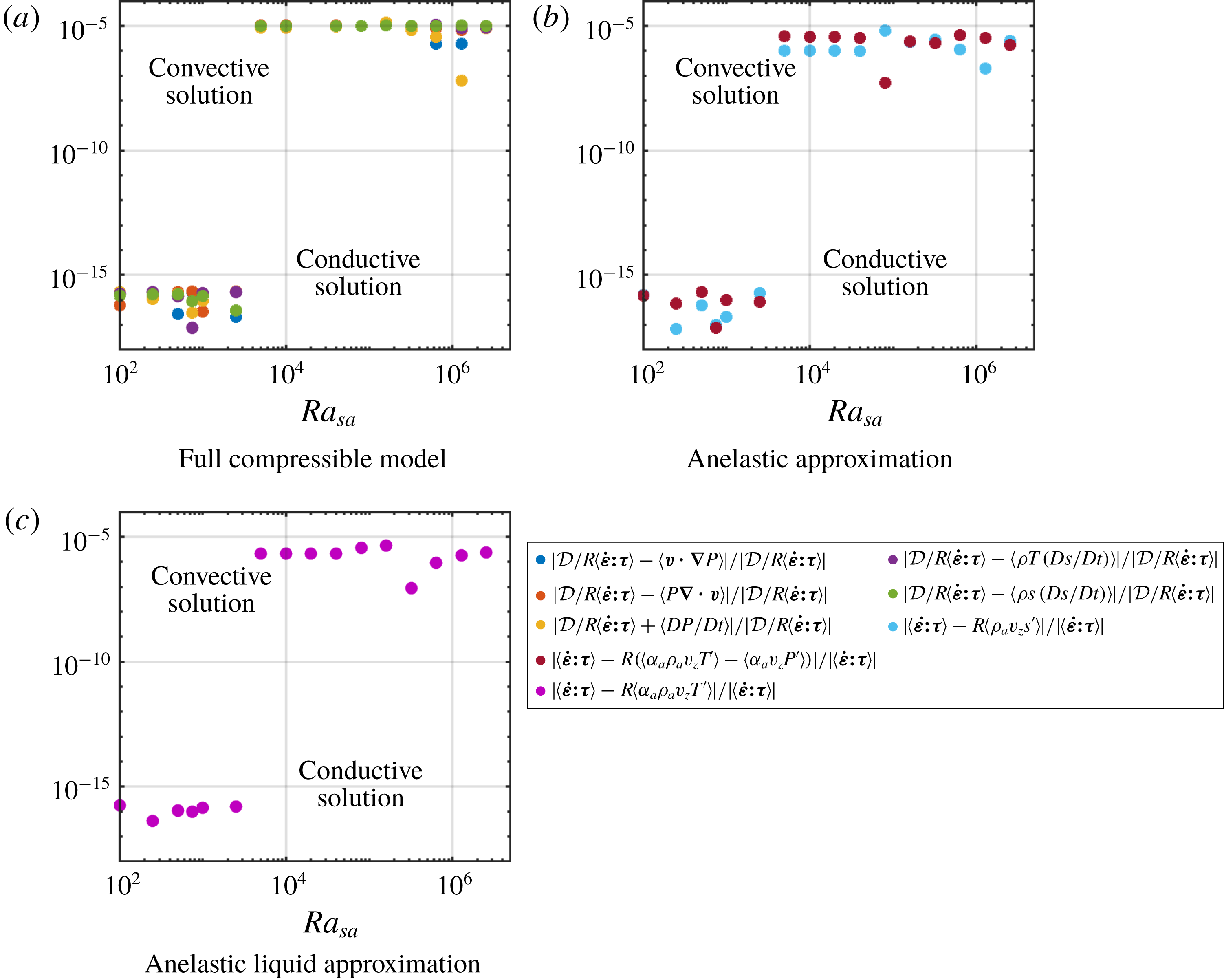
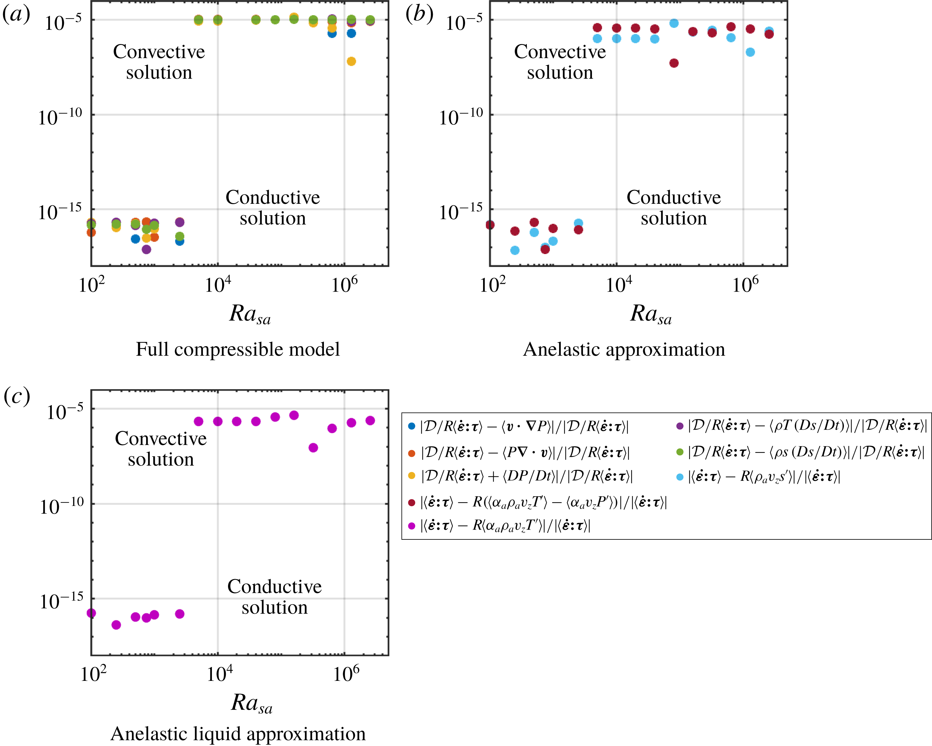
where $\langle \,\cdot \,\rangle$ denotes the time-averaged volume integral. These equalities hold for any statistically steady solution of the equations, when the time average is taken over a sufficiently long duration. Figure 2 shows that, although these equalities are not imposed in the numerical simulations, the relative differences between them turn out to be small in all cases, of the order of  $10^{-6}$ .

In the AA approximation, remembering that $\hat{\unicode[STIX]{x1D6FC}}=1$ for an ideal gas, the integrated viscous dissipation can be expressed as

(5.3) $$\begin{eqnarray}\displaystyle \langle \dot{\unicode[STIX]{x1D73A}}\boldsymbol{ : }\unicode[STIX]{x1D749}\rangle =R\langle \unicode[STIX]{x1D70C}_{a}v_{z}s^{\prime }\rangle =R\langle \unicode[STIX]{x1D6FC}_{a}\unicode[STIX]{x1D70C}_{a}v_{z}T^{\prime }\rangle -R\langle \unicode[STIX]{x1D6FC}_{a}v_{z}P^{\prime }\rangle , & & \displaystyle\end{eqnarray}$$

while in the ALA approximation, this becomes simply

(5.4) $$\begin{eqnarray}\displaystyle \langle \dot{\unicode[STIX]{x1D73A}}\boldsymbol{ : }\unicode[STIX]{x1D749}\rangle =R\langle \unicode[STIX]{x1D6FC}_{a}\unicode[STIX]{x1D70C}_{a}v_{z}T^{\prime }\rangle . & & \displaystyle\end{eqnarray}$$

The expressions are shown to be numerically equivalent (see figure 2) within a relative error always smaller than $10^{-5}$ .

Figure 2.

Computed differences between equivalent expressions for the viscous dissipation given by (5.2) for fully compressible solutions and by (5.3) and (5.4) for anelastic solutions, for $r=3$ , $\unicode[STIX]{x1D6FE}=1.4$ and $D=0.8$ ( $\unicode[STIX]{x1D716}=0.25$ ).

We also test our numerical methods against self-consistent criteria of heat transfer. Integrating horizontally and time averaging (2.11), using (2.9), (2.10) and the Gibbs equation $\text{d}h=T\,\text{d}s+\text{d}P/\unicode[STIX]{x1D70C}$ , it can be shown that the dimensionless heat flux,

(5.5) $$\begin{eqnarray}Q(z)=\overline{\unicode[STIX]{x1D70C}hv_{z}}-{\displaystyle \frac{{\mathcal{D}}}{R}}\overline{v_{j}\unicode[STIX]{x1D70F}_{z\,j}}-\overline{\unicode[STIX]{x2202}_{z}T},\end{eqnarray}$$

is conserved along the vertical direction, where $\overline{\,\cdot \,}$ denotes the time-averaged horizontal integral and $h$ is the specific enthalpy or Gibbs free energy (simply $c_{p0}T$ for an ideal gas), made dimensionless using $c_{p0}T_{0}$ . The heat flux is the sum of three components: transport of enthalpy $\overline{\unicode[STIX]{x1D70C}hv_{z}}$ , shear-stress power $-{\mathcal{D}}/R\overline{v_{j}\unicode[STIX]{x1D70F}_{z\,j}}$ and conduction $-\overline{\unicode[STIX]{x2202}_{z}T}$ . The first two components together form the ‘convective flux’. In the anelastic and anelastic liquid approximations the heat flux takes the form

(5.6) $$\begin{eqnarray}Q(z)=\overline{\unicode[STIX]{x1D70C}_{a}h^{\prime }v_{z}}-{\displaystyle \frac{{\mathcal{D}}}{R}}\overline{v_{j}\unicode[STIX]{x1D70F}_{z\,j}}-\overline{\unicode[STIX]{x2202}_{z}T},\end{eqnarray}$$

which only differs from (5.5) because $\unicode[STIX]{x1D70C}_{a}h^{\prime }$ replaces $\unicode[STIX]{x1D70C}h$ in the first term (the perturbation of enthalpy $h^{\prime }$ is simply $T^{\prime }$ for an ideal gas). The computed heat flux is indeed constant in $z$ , and its value, simply denoted $Q$ , is shown, for the fully compressible case, when the dissipation number ${\mathcal{D}}$ is varied; see figure 3. However, this value is slightly different depending on the model that has been used to calculate the solution, as can be seen in figure 3 (roughly between 5 % and 10 % lower when approximate equations are used). This fact will be used to compare the solutions obtained with different methods in § 9.

Figure 3.

Heat flux profile along the vertical direction, averaged over the horizontal direction $x$ and time, for $r=3$ and $Ra_{sa}=10\,000$ .

Figure 4.

Comparison of the structure of the patterns of convection in fully compressible FC, anelastic AA and anelastic liquid ALA approximations, for $r=3$ , $\unicode[STIX]{x1D6FE}=1.4$ and ${\mathcal{D}}=0.6$ ( $\unicode[STIX]{x1D716}=5/3$ ). Black dots indicate the presence of two symmetrical convective cells, blue dot two asymmetrical cells and green dot a single cell.

6 Visualization of convection numerical models

Before we analyse quantitatively the outcomes of our numerical models in the following sections, let us first look at the temperature and velocity fields obtained using different models and approximations, and for different values of the governing parameters: small and large superadiabatic Rayleigh numbers, small and large values of the dissipation parameter.

Some snapshots of the convection are shown in figure 4 for two values of the superadiabatic Rayleigh number, ${\mathcal{D}}=0.6$ , $r=3$ , $\unicode[STIX]{x1D6FE}=1.4$ and fully compressible model FC, anelastic approximation AA and anelastic liquid approximation ALA. Small arrows indicate the velocity field while the background colour corresponds to temperature minus the adiabatic profile (3.5). At $Ra_{sa}=2\times 10^{4}$ , all flows are steady with two convective cells of the same size in the 2-D cavity of aspect ratio 4. This pattern is denoted by a full black dot. (Full symbols denote steady convection. These symbols, full or empty, black or coloured, will be used later to refer to the various convection patterns in several phase diagrams.) However, there are subtle differences between FC, AA and ALA even at $Ra_{sa}=2\times 10^{4}$ : the background temperature is hotter for AA (and ALA to a lesser extent). This is most probably due to the asymmetry of the thermal boundary layers, as discussed in § 8. At $Ra_{sa}=4\times 10^{4}$ , the pattern is unchanged for the FC flow but it has changed for AA (two convective cells of different size, full blue dot) and ALA (one big cell, full green dot). That change in pattern implies also a change in heat transfer. At slightly larger $Ra_{sa}$ the transition to unsteady convection will also occur for different values of $Ra_{sa}$ depending on the model of convection.

Fully compressible calculations at larger values of the Rayleigh number, $Ra_{sa}=3.2\times 10^{5}$ and $Ra_{sa}=1.28\times 10^{6}$ , and for two values of the dissipation number, ${\mathcal{D}}=0.2$ and ${\mathcal{D}}=0.9$ , are shown in figure 5, for a temperature ratio $r=3$ and $\unicode[STIX]{x1D6FE}=1.4$ . The corresponding solutions are all unsteady. The structures of temperature become thinner and more chaotic at large $Ra_{sa}$ . It can be seen also that the bulk of the fluid is shifted towards hot values of superadiabatic temperature for ${\mathcal{D}}=0.9$ , with a strong thick cold boundary layer at the top and a weak hot boundary layer at the bottom.

Figure 5.

Structure of the plumes for the superadiabatic temperature $T_{sa}$ in the fully compressible model for $r=3$ and $\unicode[STIX]{x1D6FE}=1.4$ .

7 Average temperature profiles

Figure 6.

Average temperature profiles from the fully compressible model FC, for $\unicode[STIX]{x1D6FE}=1.4$ and a temperature ratio $r=3$ . The value of the dissipation number is ${\mathcal{D}}=0.2$ ( $\unicode[STIX]{x1D716}=4$ ) on (a) and ${\mathcal{D}}=0.8$ ( $\unicode[STIX]{x1D716}=0.25$ ) on (b). The profiles are shown for various values of the superadiabatic Rayleigh number (reference adiabatic profile shown as dashed line).

Figure 7.

Average temperature profiles obtained from the fully compressible FC, anelastic AA and anelastic liquid ALA models, for $Ra_{sa}=320\,000$ , $\unicode[STIX]{x1D6FE}=1.4$ and $r=3$ . The value of the dissipation number is ${\mathcal{D}}=0.2$ ( $\unicode[STIX]{x1D716}=4$ ) on (a) and ${\mathcal{D}}=0.8$ ( $\unicode[STIX]{x1D716}=0.25$ ) on (b) (reference adiabatic profile shown as dashed line).

A selection of time-averaged and horizontally averaged temperature profiles are shown in figures 6 and 7. In figure 6, the average profiles are those obtained with the fully compressible model FC, for a heat capacity ratio equal to $\unicode[STIX]{x1D6FE}=1.4$ and a temperature ratio $r=3$ between the bottom and top imposed temperatures. It can be observed that the profiles follow more or less the adiabatic reference profile in the bulk of the cavity with boundary layers where the temperature profiles bend to match the boundary conditions. As the superadiabatic Rayleigh number is increased, the thickness of the boundary layers is reduced. On the left-hand side, corresponding to a dissipation number ${\mathcal{D}}=0.2$ , the profiles are all close to the reference adiabatic profile in the bulk of the fluid. It is reminded here that the adiabatic reference profile is such that the superadiabatic differences with the top and bottom temperatures are equal. On the contrary, on the right-hand side, corresponding to ${\mathcal{D}}=0.8$ , the profiles follow a line parallel to, but distinct from, the adiabatic reference profile in the bulk of the flow. This means that the profiles still possess a temperature gradient in accordance with the adiabatic gradient, but that the actual profile is shifted by a constant temperature offset: a connected observation is that the temperature jump in the thermal boundary layers are not equal at the top and at the bottom since $Q_{top}=Q_{bot}$ (see (5.6)). More often, the temperature jump across the upper boundary is larger than that across the lower boundary layer. This point will be discussed in § 8.

In figure 7, the profiles obtained from different models (FC, AA and ALA) are shown for comparison. The superadiabatic Rayleigh number is equal to 320 000, $\unicode[STIX]{x1D6FE}=1.4$ and $r=3$ . Similarly to figure 6, the dissipation number is equal to 0.2 on the left-hand side and to 0.8 on the right-hand side. For ${\mathcal{D}}=0.2$ , on the left-hand side, the three profiles corresponding to the fully compressible FC model, anelastic AA and anelastic liquid ALA approximations do not follow the same adiabat in the bulk of the flow. The fully compressible profile has nearly no temperature offset compared to the adiabatic reference profile, while the anelastic approximation has a significant positive temperature offset, and the anelastic liquid a smaller offset. On the right-hand side, for ${\mathcal{D}}=0.8$ , all three profiles follow the same adiabat, which is offset compared to the adiabatic reference profile. It is indeed expected that the anelastic approximations do a better job at reproducing the fully compressible results when the dissipation number is large and close to its maximum ( ${\mathcal{D}}=1$ for $r=3$ ), because the superadiabatic temperature difference is small compared to the adiabatic temperature difference, thus reducing the uncertainty on the possible shift of the adiabatic profile.

Another feature of the average temperature profile is that it shows overshoots at the outer part of the boundary layers. This is more clearly visible in the case of ${\mathcal{D}}=0.2$ in figures 6 and 7. It can also be seen that the overshoots depend on the numerical model used (see figure 7): the anelastic profile AA has nearly no overshoot close to the top boundary layer while it is larger than its fully compressible FC counterpart near the bottom boundary layer.

Figure 8.

Typical horizontally averaged temperature profile $\overline{T}(z)$ , reference adiabatic profile $T_{a}(z)$ , shifted adiabatic temperature profile $T_{a}(z)+\unicode[STIX]{x1D6FD}$ and boundary layer amplitudes ( $\unicode[STIX]{x1D6FF}T_{sab}$ at the bottom, $\unicode[STIX]{x1D6FF}T_{sat}$ at the top) and thicknesses ( $\unicode[STIX]{x1D6FF}_{b}$ at the bottom, $\unicode[STIX]{x1D6FF}_{t}$ at the top). The dashed profile $T_{bl}(z)$ is an idealized piecewise-linear profile, with linear core and linear boundary layers.

In order to understand analytically our numerical results, we consider a simplified representation of the average temperature profile, in the form of a piecewise-linear function of $z$ , one linear part in each boundary layer and a third one in the bulk of the fluid. This function, denoted $T_{bl}(z)$ (for ‘boundary layers’), is shown in figure 8. The bulk linear part follows the adiabatic gradient (slope ${\mathcal{D}}$ ), while the linear parts in the boundary layers are such that the total average heat flux is conducted along their gradient (slope $Q$ ). This schematic profile indeed captures the typical temperature profiles of convecting compressible fluids whatever the approximations that are used (see figure 6 or 7) with the exceptions of the slight temperature overshoots that occur at the transitions between the conductive boundary layers and the adiabatic bulk. The profile must be anchored at the boundary conditions on temperatures (2.18) set by the ratio $r$ . The last free parameter is the temperature offset $\unicode[STIX]{x1D6FD}$ of the adiabat in the core of the fluid. The analytical expression of this empirical profile is

(7.1) $$\begin{eqnarray}\displaystyle \left.\begin{array}{@{}c@{}}T_{bl}(z)=1+{\textstyle \frac{1}{2}}\unicode[STIX]{x1D6FF}T-zQ,\quad 0<z<\unicode[STIX]{x1D6FF}_{b},\\ T_{bl}(z)=1+\unicode[STIX]{x1D6FD}-{\mathcal{D}}(z-{\textstyle \frac{1}{2}}),\quad \unicode[STIX]{x1D6FF}_{b}<z<1-\unicode[STIX]{x1D6FF}_{t},\\ T_{bl}(z)=1-{\textstyle \frac{1}{2}}\unicode[STIX]{x1D6FF}T-Q(z-1),\quad 1-\unicode[STIX]{x1D6FF}_{t}<z<1,\end{array}\right\} & & \displaystyle\end{eqnarray}$$

where $\unicode[STIX]{x1D6FF}T=2(r-1)/(r+1)$ . The expressions for the thickness of the boundary layers are obtained by continuity of the temperature profile,

(7.2a,b ) $$\begin{eqnarray}\unicode[STIX]{x1D6FF}_{b}={\displaystyle \frac{(\unicode[STIX]{x1D6FF}T-{\mathcal{D}})/2-\unicode[STIX]{x1D6FD}}{Q-{\mathcal{D}}}},\quad \unicode[STIX]{x1D6FF}_{t}={\displaystyle \frac{(\unicode[STIX]{x1D6FF}T-{\mathcal{D}})/2+\unicode[STIX]{x1D6FD}}{Q-{\mathcal{D}}}}.\end{eqnarray}$$

Those expressions can be further simplified when using the notation $\unicode[STIX]{x1D6FF}T_{sa}=\unicode[STIX]{x1D6FF}T-{\mathcal{D}}$ and $Q_{sa}=Q-{\mathcal{D}}$ , for the total superadiabatic temperature difference and superadiabatic heat flux, respectively. The total superadiabatic temperature difference $\unicode[STIX]{x1D6FF}T_{sa}$ is the sum of the superadiabatic temperature differences occurring across the bottom and the top boundary layers $\unicode[STIX]{x1D6FF}T_{sa}=\unicode[STIX]{x1D6FF}T_{sab}+\unicode[STIX]{x1D6FF}T_{sat}$ :

(7.3a,b ) $$\begin{eqnarray}\unicode[STIX]{x1D6FF}_{b}={\displaystyle \frac{\unicode[STIX]{x1D6FF}T_{sa}/2-\unicode[STIX]{x1D6FD}}{Q_{sa}}},\quad \unicode[STIX]{x1D6FF}_{t}={\displaystyle \frac{\unicode[STIX]{x1D6FF}T_{sa}/2+\unicode[STIX]{x1D6FD}}{Q_{sa}}}.\end{eqnarray}$$

We will see in § 8 that various numerical results will be recovered from this simple profile when we derive an analytical expression of the offset $\unicode[STIX]{x1D6FD}$ as a function of the parameters $r$ and  ${\mathcal{D}}$ .

8 An empirical rationale

Let us consider the general asymmetry of the temperature profile. We attempt here to derive a rationale to explain the relative difference between the top and bottom boundary layer thicknesses. We shall then infer the consequences of this asymmetry on dissipation, entropy sources and heat flux. The ratio of the boundary layer thicknesses $x=\unicode[STIX]{x1D6FF}_{t}/\unicode[STIX]{x1D6FF}_{b}$ is also equal to the ratio of superadiabatic temperature jumps $x=\unicode[STIX]{x1D6FF}T_{sat}/\unicode[STIX]{x1D6FF}T_{sab}$ (because the thermal conductivity is uniform, see figure 8) and takes the following expression:

(8.1) $$\begin{eqnarray}x={\displaystyle \frac{\unicode[STIX]{x1D6FF}_{t}}{\unicode[STIX]{x1D6FF}_{b}}}={\displaystyle \frac{\unicode[STIX]{x1D6FF}T_{sat}}{\unicode[STIX]{x1D6FF}T_{sab}}}={\displaystyle \frac{(\unicode[STIX]{x1D6FF}T-{\mathcal{D}})/2+\unicode[STIX]{x1D6FD}}{(\unicode[STIX]{x1D6FF}T-{\mathcal{D}})/2-\unicode[STIX]{x1D6FD}}}.\end{eqnarray}$$

We have determined the average temperature profile of our numerical simulations and found the closest adiabat followed in the bulk of the fluid. This provides both the offset $\unicode[STIX]{x1D6FD}$ and the ratio $x$ of the thicknesses of top to bottom boundary layers. This value is plotted in figure 9 as a function of the dissipation number for different sets of parameters and different approximations. Contrary to the incompressible finite-Prandtl-number experiments described in Wu & Libchaber (Reference Wu and Libchaber1991), the values of the ratio $x$ are mainly larger than unity. As we shall see below, the relative thickness of the boundary layers might be due to the relative thermal diffusivity, hence due to density in our simulations with uniform thermal conductivity (and heat capacity $c_{p0}$ for ideal gases). In Wu & Libchaber (Reference Wu and Libchaber1991), density was affected by temperature only – hot at the bottom, cold at the top – producing a lower density at the bottom than at the top. In our case, pressure effects dominate (except for small values of ${\mathcal{D}}$ ) – large pressure at the bottom, low pressure at the top leads to a larger density at the bottom than at the top.

Figure 9.

The ratio of boundary layer thicknesses $x$ plotted against the dissipation number. Crosses correspond to fully compressible calculations; circles to anelastic modelling. Blue points correspond to $r=3$ , $\unicode[STIX]{x1D6FE}=1.4$ and different superadiabatic Rayleigh numbers; brown points to $r=3$ , $\unicode[STIX]{x1D6FE}=5/3$ and $Ra_{sa}=320\,000$ ; black points to $r=10$ , $\unicode[STIX]{x1D6FE}=5/3$ and $Ra_{sa}=320\,000$ ; finally yellow points correspond to $r=10$ , $\unicode[STIX]{x1D6FE}=1.4$ , $Ra_{sa}=10^{4}$ , $Ra_{sa}=10^{5}$ and $Ra_{sa}=10^{6}$ .

Now, we are going to use an empirical rule – a rationale – along with the piecewise-linear profile defined above, that will enable us to model some of our numerical results. In fact, we are first going to test three different rationales against the numerical results and select the most satisfactory. This is inspired by the work of Wu & Libchaber (Reference Wu and Libchaber1991), where they also tested different hypotheses against experimental results in the context of non-Boussinesq, nearly incompressible Rayleigh–Bénard convection.

The first hypothesis consists in assuming that the Rayleigh number of each boundary layer is critical: for our purpose, we simply assume that they always take the same value. The second hypothesis is to be found in Wu & Libchaber (Reference Wu and Libchaber1991) (where they also tested the constant Rayleigh number hypothesis) and consists in assuming that the top and bottom potential temperature differences are equal: the potential temperature difference is such that it makes the Rayleigh number critical. Finally, we introduce a third rationale, consisting in assuming that the time scale of the development of the boundary layers is identical at the top and bottom.

The ratio of top, $Ra_{t}$ , to bottom, $Ra_{b}$ , boundary layer Rayleigh numbers is now evaluated considering that both thermal conductivity and viscosity are uniform:

(8.2) $$\begin{eqnarray}{\displaystyle \frac{Ra_{t}}{Ra_{b}}}={\displaystyle \frac{\unicode[STIX]{x1D6FC}_{t}\unicode[STIX]{x1D70C}_{t}^{2}\unicode[STIX]{x1D6FF}T_{sat}\unicode[STIX]{x1D6FF}_{t}^{3}}{\unicode[STIX]{x1D6FC}_{b}\unicode[STIX]{x1D70C}_{b}^{2}\unicode[STIX]{x1D6FF}T_{sab}\unicode[STIX]{x1D6FF}_{b}^{3}}}=\left({\displaystyle \frac{P_{t}}{P_{b}}}\right)^{2}\left({\displaystyle \frac{T_{b}}{T_{t}}}\right)^{3}x^{4}.\end{eqnarray}$$

Here all values evaluated at the top have a subscript $t$ and those at the bottom a subscript $b$ . As we want to compare different rationales, we also make the choice to compare quantities simply proportional to $x$ , so that we shall take the expression (8.2) to the power one-fourth. Hence, the following function $R1$ corresponds to the ratio of the Rayleigh numbers to the power one-fourth:

(8.3) $$\begin{eqnarray}R1=\left({\displaystyle \frac{P_{t}}{P_{b}}}\right)^{1/2}\left({\displaystyle \frac{T_{b}}{T_{t}}}\right)^{3/4}x.\end{eqnarray}$$

From our numerical calculations, if we can define the top and bottom pressures and temperatures, which we discuss later, and evaluate $x$ by fitting the average temperature profile with the closest adiabat line, we can then compute $R1$ , and values close to unity would indicate that the first rationale is a good representation of the simulations and values departing from unity that the Rayleigh numbers are not equal in both boundary layers.

We follow a similar path for the second rationale. The ratio of potential temperature differences can be written as

(8.4) $$\begin{eqnarray}{\displaystyle \frac{\unicode[STIX]{x1D703}_{b}}{\unicode[STIX]{x1D703}_{t}}}={\displaystyle \frac{\unicode[STIX]{x1D6FC}_{t}\unicode[STIX]{x1D70C}_{t}^{2}\unicode[STIX]{x1D6FF}_{t}^{3}}{\unicode[STIX]{x1D6FC}_{b}\unicode[STIX]{x1D70C}_{b}^{2}\unicode[STIX]{x1D6FF}_{b}^{3}}}=\left({\displaystyle \frac{P_{t}}{P_{b}}}\right)^{2}\left({\displaystyle \frac{T_{b}}{T_{t}}}\right)^{3}x^{3},\end{eqnarray}$$

leading to the following function $R2$ for the second rationale

(8.5) $$\begin{eqnarray}R2=\left({\displaystyle \frac{P_{t}}{P_{b}}}\right)^{2/3}{\displaystyle \frac{T_{b}}{T_{t}}}x.\end{eqnarray}$$

If those ratios are close to unity, then potential temperature differences for both boundary layers are indeed nearly equal.

In the third rationale, we consider that the top and bottom boundary layers develop over the same time scale $\unicode[STIX]{x1D70F}$ . Thus their typical diffusion thickness $\unicode[STIX]{x1D6FF}\sim \sqrt{\unicode[STIX]{x1D705}\unicode[STIX]{x1D70F}}$ (where $\unicode[STIX]{x1D705}$ is the thermal diffusivity) depends explicitly on density $\unicode[STIX]{x1D6FF}\sim \sqrt{k/(\unicode[STIX]{x1D70C}c_{p})\unicode[STIX]{x1D70F}}$ . Hence the ratio of boundary layer thicknesses is inversely proportional to the square root of the density ratio. From this point, we can build the function $R3$ corresponding to this rationale:

(8.6) $$\begin{eqnarray}R3=\left({\displaystyle \frac{\unicode[STIX]{x1D70C}_{t}}{\unicode[STIX]{x1D70C}_{b}}}\right)^{1/2}x=\left({\displaystyle \frac{P_{t}}{P_{b}}}\right)^{1/2}\left({\displaystyle \frac{T_{b}}{T_{t}}}\right)^{1/2}x.\end{eqnarray}$$

Again, values close to unity for these functions is a validation of the third rationale, based on a constant development duration for the thermal boundary layers.

Like Wu & Libchaber (Reference Wu and Libchaber1991), we consider the average within a boundary layer when we need to evaluate a physical property relative to that boundary layer. However, the fully compressible case FC and an anelastic model (AA or ALA) are treated differently: for anelastic models, all quantities are evaluated on the adiabatic reference profile, so that physical quantities in a particular boundary layer must be evaluated at the conditions of the adiabatic reference profile using (3.5) and (3.7). In addition, we consider their value at the boundaries, which is only very slightly different from their value in the middle of the thin boundary layers so that, for the AA and ALA models, we can consider that

(8.7) $$\begin{eqnarray}\left.\begin{array}{@{}c@{}}T_{t}=1-{\mathcal{D}}/2,\\ T_{b}=1+{\mathcal{D}}/2,\\ P_{t/b}={\displaystyle \frac{{\mathcal{D}}}{T_{b}^{\unicode[STIX]{x1D6FE}/(\unicode[STIX]{x1D6FE}-1)}-T_{t}^{\unicode[STIX]{x1D6FE}/(\unicode[STIX]{x1D6FE}-1)}}}T_{t/b}^{\unicode[STIX]{x1D6FE}/(\unicode[STIX]{x1D6FE}-1)}.\end{array}\right\}\end{eqnarray}$$

From our anelastic computations and using those expressions for the top and bottom pressures and temperature, we can therefore evaluate the $R1_{A}$ , $R2_{A}$ and $R3_{A}$ following (8.3), (8.5) and (8.6), where we add the subscript $A$ for ‘anelastic’.

In the case of fully compressible results FC, we take into account the thermal boundary layers to evaluate temperatures $T_{b}$ and $T_{t}$ , but we can safely approximate the exact pressure by the pressure along the adiabat. In addition, we now need to take the offset $\unicode[STIX]{x1D6FD}$ into account. Instead of the anelastic estimates (8.7), for the FC case, we must now use

(8.8) $$\begin{eqnarray}\left.\begin{array}{@{}c@{}}T_{t}={\displaystyle \frac{1}{2}}\left(1+\unicode[STIX]{x1D6FD}-{\mathcal{D}}/2+{\displaystyle \frac{2}{r+1}}\right),\\ T_{b}={\displaystyle \frac{1}{2}}\left(1+\unicode[STIX]{x1D6FD}+{\mathcal{D}}/2+{\displaystyle \frac{2r}{r+1}}\right),\\ P_{t}={\displaystyle \frac{{\mathcal{D}}}{(1+\unicode[STIX]{x1D6FD}+{\mathcal{D}}/2)^{\unicode[STIX]{x1D6FE}/(\unicode[STIX]{x1D6FE}-1)}-(1+\unicode[STIX]{x1D6FD}-{\mathcal{D}}/2)^{\unicode[STIX]{x1D6FE}/(\unicode[STIX]{x1D6FE}-1)}}}(1+\unicode[STIX]{x1D6FD}-{\mathcal{D}}/2)^{\unicode[STIX]{x1D6FE}/(\unicode[STIX]{x1D6FE}-1)},\\ P_{b}={\displaystyle \frac{{\mathcal{D}}}{(1+\unicode[STIX]{x1D6FD}+{\mathcal{D}}/2)^{\unicode[STIX]{x1D6FE}/(\unicode[STIX]{x1D6FE}-1)}-(1+\unicode[STIX]{x1D6FD}-{\mathcal{D}}/2)^{\unicode[STIX]{x1D6FE}/(\unicode[STIX]{x1D6FE}-1)}}}(1+\unicode[STIX]{x1D6FD}+{\mathcal{D}}/2)^{\unicode[STIX]{x1D6FE}/(\unicode[STIX]{x1D6FE}-1)},\end{array}\right\}\end{eqnarray}$$

where $\unicode[STIX]{x1D6FD}$ is obtained from $x$ by inverting (8.1):

(8.9) $$\begin{eqnarray}\unicode[STIX]{x1D6FD}={\displaystyle \frac{\unicode[STIX]{x1D6FF}T-{\mathcal{D}}}{2}}\,{\displaystyle \frac{x-1}{x+1}}.\end{eqnarray}$$

The pressure expressions are computed along the adiabat taking into account the appropriate $\unicode[STIX]{x1D6FD}$ offset of the temperature (in agreement with (3.7)).

Figure 10.

The three quantities corresponding to the three different rationales plotted against the dissipation number. Crosses correspond to fully compressible calculations; circles to anelastic modelling. Blue points correspond to $r=3$ , $\unicode[STIX]{x1D6FE}=1.4$ and different superadiabatic Rayleigh numbers; brown points to $r=3$ , $\unicode[STIX]{x1D6FE}=5/3$ and $Ra_{sa}=320\,000$ ; black points to $r=10$ , $\unicode[STIX]{x1D6FE}=5/3$ and $Ra_{sa}=320\,000$ ; finally yellow points correspond to $r=10$ , $\unicode[STIX]{x1D6FE}=1.4$ , $Ra_{sa}=10^{4}$ , $Ra_{sa}=10^{5}$ and $Ra_{sa}=10^{6}$ .

All functions $R1$ , $R1_{A}$ , $R2$ , $R2_{A}$ , $R3$ and $R3_{A}$ are plotted in figure 10. It can be seen that the third rationale is slightly better than the second or first: all points (AA and FC) are closer to unity in the range of our numerical simulations. Hence, in the following, we are going to use the third rationale, based on a constant time scale of boundary layer development, i.e. deduce $x$ from

(8.10) $$\begin{eqnarray}x=\left({\displaystyle \frac{\unicode[STIX]{x1D70C}_{b}}{\unicode[STIX]{x1D70C}_{t}}}\right)^{1/2}=\left({\displaystyle \frac{P_{b}}{P_{t}}}\right)^{1/2}\left({\displaystyle \frac{T_{t}}{T_{b}}}\right)^{1/2}\end{eqnarray}$$

in the anelastic and fully compressible cases using (8.7) or (8.8), to derive conclusions regarding the dependence of the heat flux and viscous dissipation versus the dissipation number. In the anelastic case, the expression (8.10) provides $x$ explicitly in terms of ${\mathcal{D}}$ and $\unicode[STIX]{x1D6FE}$ . However, this is not the case for the fully compressible expression due to the presence of $\unicode[STIX]{x1D6FD}$ , which is itself linked to $x$ by equation (8.9): one can use an iterative numerical method in order to obtain finally $x$ as a function of ${\mathcal{D}}$ , $\unicode[STIX]{x1D6FE}$ and  $r$ .

The dependence of the Nusselt number versus the dissipation number (the numerical results are found in figures 12 and 13) can be derived from our rationale. Because the isentropic (or adiabatic) profile represents an equilibrium state of the fluid in terms of buoyancy, we decompose the total heat flux into a flux conducted along the adiabat, $Q_{a}=\unicode[STIX]{x0394}T_{a}={\mathcal{D}}$ , and a so-called superadiabatic heat flux, $Q_{sa}=Q-Q_{a}$ . The superadiabatic heat flux is driven by the superadiabatic temperature difference $\unicode[STIX]{x0394}T-\unicode[STIX]{x0394}T_{a}$ and we introduce a superadiabatic Nusselt number defined as the ratio of the superadiabatic heat flux to the flux conducted by the superadiabatic temperature difference

(8.11) $$\begin{eqnarray}Nu_{sa}={\displaystyle \frac{Q_{sa}}{\unicode[STIX]{x0394}T_{sa}}}.\end{eqnarray}$$

From figure 8, the dimensionless superadiabatic heat flux $Q_{sa}$ can be written as

(8.12) $$\begin{eqnarray}Q_{sa}={\displaystyle \frac{\unicode[STIX]{x1D6FF}T_{sat}}{\unicode[STIX]{x1D6FF}_{t}}}.\end{eqnarray}$$

Using the definition of $x$ , from (8.1), and expressing the total dimensionless superadiabatic temperature difference $\unicode[STIX]{x1D6FF}T_{sa}=\unicode[STIX]{x1D6FF}T_{sat}+\unicode[STIX]{x1D6FF}T_{sab}$ , we have

(8.13) $$\begin{eqnarray}\unicode[STIX]{x1D6FF}T_{sat}={\displaystyle \frac{x}{1+x}}\unicode[STIX]{x1D6FF}T_{sa}.\end{eqnarray}$$

Furthermore, we adopt an extended version of our rationale. We now assume that the time scale for the development of the top and bottom boundary layers depends on the superadiabatic Rayleigh number only (and not on the dissipation number ${\mathcal{D}}$ , nor $\unicode[STIX]{x1D6FE}$ , nor $r$ ). This implies that the boundary layer thickness is inversely proportional to the square root of density, so that (8.12) and (8.13) lead to

(8.14) $$\begin{eqnarray}Nu_{sa}={\displaystyle \frac{Q_{sa}}{\unicode[STIX]{x1D6FF}T_{sa}}}=2{\displaystyle \frac{x}{1+x}}\sqrt{\unicode[STIX]{x1D70C}_{t}}\,Nu_{0},\end{eqnarray}$$

where $Nu_{0}$ is the Nusselt number of the anelastic calculation AA at small dissipation number ${\mathcal{D}}\sim 0$ and same Rayleigh number (for which density is unity everywhere, including in the top boundary layer). This last expression can be made symmetrical since the superadiabatic heat flux can be expressed in terms of the bottom parameters $Q_{sa}=\unicode[STIX]{x1D6FF}T_{sab}/\unicode[STIX]{x1D6FF}_{b}$ . This would lead to

(8.15) $$\begin{eqnarray}Nu_{sa}=2{\displaystyle \frac{1}{1+x}}\sqrt{\unicode[STIX]{x1D70C}_{b}}\,Nu_{0}.\end{eqnarray}$$

Taking the geometric average of (8.14) and (8.15), and inserting the definition of $x$ (see (8.10)), gives the following symmetrical expression:

(8.16) $$\begin{eqnarray}Nu_{sa}=2{\displaystyle \frac{\sqrt{\unicode[STIX]{x1D70C}_{b}\unicode[STIX]{x1D70C}_{t}}}{\sqrt{\unicode[STIX]{x1D70C}_{b}}+\sqrt{\unicode[STIX]{x1D70C}_{t}}}}Nu_{0}={\displaystyle \frac{2}{\sqrt{1-\unicode[STIX]{x1D6FE}^{-1}}}}{\displaystyle \frac{\sqrt{P_{b}P_{t}}}{\sqrt{P_{b}T_{t}}+\sqrt{P_{t}T_{b}}}}Nu_{0}.\end{eqnarray}$$

Now, the above expression (8.16) is evaluated differently for anelastic calculations $Nu_{saAA}$ (where pressures and temperatures are given by (8.7)) and for fully compressible calculations $Nu_{saFC}$ for which we use (8.8). We will see in § 9 that the rationale indeed correctly describes the variation of the Nusselt number with the dissipation number.

9 Heat flux

We now analyse the outcome of the numerical calculations in terms of global heat flux transferred through the layer. We have run calculations for a temperature ratio $r=3$ and some others for $r=10$ . The ratio of heat capacities has been set to $\unicode[STIX]{x1D6FE}=1.4$ , corresponding to diatomic gases. Ranges of the other two available dimensionless numbers, ${\mathcal{D}}$ and $Ra_{sa}$ , have been investigated. Convection can only occur when the conductive gradient $a=2(r-1)/(r+1)$ corresponding to the difference of the imposed temperatures (2.18) is larger than the adiabatic gradient ${\mathcal{D}}$ . Equivalently, for a given value of $r$ , the value of ${\mathcal{D}}$ must lie within the interval $[0;{\mathcal{D}}_{max}]$ , where ${\mathcal{D}}_{max}$ has been defined in (2.22). For $r=3$ the dissipation number ${\mathcal{D}}$ is in $[0;1]$ . For $r=10$ , this interval is $[0;18/11]$ . When ${\mathcal{D}}$ exceeds ${\mathcal{D}}_{max}$ , the fluid is stably stratified and no convection can develop. The range of $Ra_{sa}$ is limited by resolution and calculation time.

Figure 11.

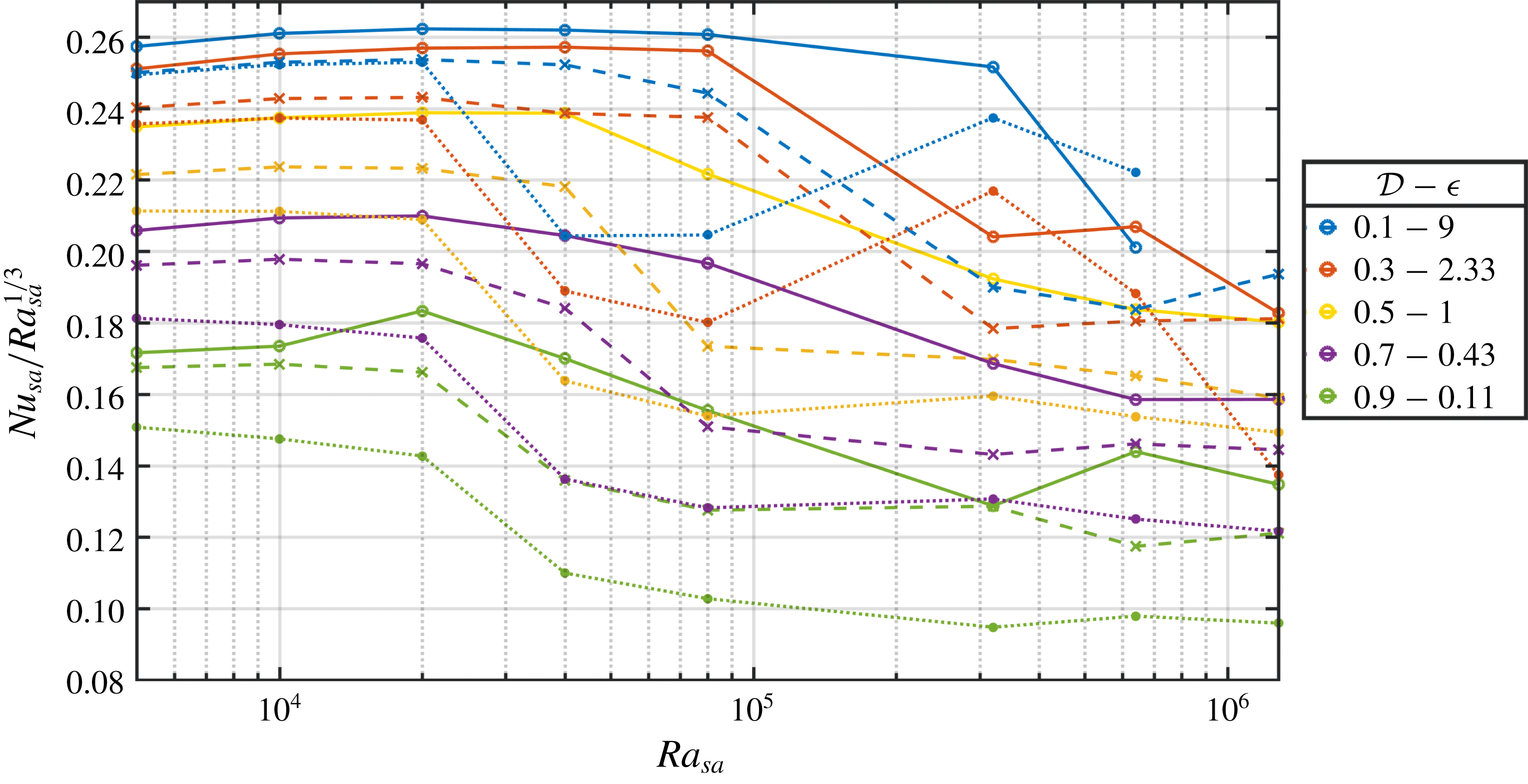
Superadiabatic Nusselt number $Nu_{sa}=Q_{sa}/\unicode[STIX]{x0394}T_{sa}$ , divided by $Ra_{sa}^{1/3}$ , as a function of $Ra_{sa}$ for fully compressible calculations (solid lines), anelastic approximation (dashed lines) and anelastic liquid approximation (dotted lines), for $r=3$ , $\unicode[STIX]{x1D6FE}=1.4$ and a range of values of the dissipation number ${\mathcal{D}}$ .

Figure 12.

Superadiabatic Nusselt number $Nu_{sa}=Q_{sa}/\unicode[STIX]{x0394}T_{sa}$ as a function of ${\mathcal{D}}$ for fully compressible calculations (solid lines) and anelastic approximation (dashed lines), for $r=3$ , $\unicode[STIX]{x1D6FE}=1.4$ and a range of values of the superadiabatic Rayleigh number $Ra_{sa}$ . The black lines correspond to the ‘rationale’ expression (8.16) derived in § 8 for the fully compressible case (full lines (8.8)) and anelastic approximation (dashed lines (8.7)). The free parameter $Nu_{0}$ is chosen such that the anelastic profile has the best fit with the anelastic numerical results.

9.1 Fully compressible FC versus anelastic approximation AA results

The value of the heat flux is compared between the fully compressible calculations and the corresponding anelastic approximation. For convection at infinite $Pr$ number, it is believed that $Nu_{sa}\propto Ra_{sa}^{1/3}$ in the Boussinesq approximation (Malkus Reference Malkus1954; Grossmann & Lohse Reference Grossmann and Lohse2000) and we shall plot our compressible results relative to the same scaling. In figure 11, we plot the superadiabatic Nusselt number scaled with $Ra_{sa}^{1/3}$ , for different values of the dissipation number ${\mathcal{D}}$ . The results for the fully compressible model and anelastic approximation are plotted together, for an imposed temperature ratio $r=3$ . The scaling $Nu_{sa}\sim Ra_{sa}^{1/3}$ is roughly correct for all values of ${\mathcal{D}}$ , up to the maximum ${\mathcal{D}}=1$ for $r=3$ . More precisely, we identify a transition, near $Ra_{sa}=10^{5}$ , with a decrease of the prefactor of 25 $\,\%$ in the $Ra_{sa}^{1/3}$ scaling. This corresponds to the change from a steady to an unsteady convection regime (see below). This transition, observed here in 2-D calculations, is likely to occur for lower Rayleigh numbers in three-dimensional (3-D) calculations. The same results of superadiabatic Nusselt numbers are plotted in figure 12, as a function of ${\mathcal{D}}$ , for several values of the superadiabatic Rayleigh number $Ra_{sa}$ . The values of $Nu_{sa}$ are constant at small ${\mathcal{D}}$ and decline for larger ${\mathcal{D}}$ by approximately 40 % when ${\mathcal{D}}=1$ . The effect of the dissipation number seems to be independent of the superadiabatic Rayleigh number. We also plot in figures 11 and 12 the predictions (8.16) for fully compressible model (using (8.8)) and for the anelastic approximation (using (8.7)), obtained from the heuristic reasoning developed in § 8, based on the relative development of the top and bottom boundary layers. The numerical Nusselt numbers follow quite well the predictions of this rationale. The value of $Nu_{sa}$ for $r=10$ has a similar behaviour, as can be seen in figure 13, where $Nu_{sa}$ is represented as a function of ${\mathcal{D}}$ up to the maximum ${\mathcal{D}}=2(r-1)/(r+1)$ for the anelastic calculations.

Figure 13.

Superadiabatic Nusselt number $Nu_{sa}=Q_{sa}/\unicode[STIX]{x0394}T_{sa}$ as a function of ${\mathcal{D}}$ for the anelastic approximation with different values of $\unicode[STIX]{x1D6FE}$ and a range of values of the superadiabatic Rayleigh number $Ra_{sa}$ . Black curves correspond to the analytic expression (8.16), using (8.7).

On both figures 11 and 12, we can observe that the Nusselt numbers computed with the fully compressible method are larger than those computed using the anelastic approximation. This is made clear in figure 14 on which we represent the relative difference in the superadiabatic Nusselt numbers $(Nu_{sa}^{FC}-Nu_{sa}^{AA})/Nu_{sa}^{FC}$ on a colour scale in the plane ${\mathcal{D}}$ – $Ra_{sa}$ , where $Nu_{sa}^{FC}$ is the superadiabatic Nusselt number obtained with the fully compressible method, while $Nu_{sa}^{AA}$ is obtained using the anelastic approximation. Nearly all values are positive (red colour) and indicate that the heat flow is 10 %–20 % larger than what is obtained by the anelastic approximation. Moreover, we also indicate the points in this parameter space ${\mathcal{D}}$ – $Ra_{sa}$ where numerical calculations have been performed. Full circles indicate a regime of steady convection, empty circles an unsteady regime, for fully compressible results FC and anelastic results AA, left and right symbols, respectively. The colour of the points depends on the spatial structure of convection as in figure 4: two symmetric rolls (black), two asymmetric rolls (blue), one large convection roll (green), or indefinite (grey). A region of maximum relative difference (intense red, positive) of the Nusselt number corresponds to the line $Ra=8\times 10^{4}$ , just below $10^{5}$ . It basically corresponds to the region where the anelastic results have already undergone transition to unsteady convective rolls (empty symbols), while fully compressible results are still steady (full symbols). This is also visible in figure 11, where the transition to a smaller prefactor occurs at a smaller Rayleigh number for anelastic solutions compared to fully compressible solutions. That transition is dependent on the 2-D nature of the simulations and would likely occur at small Rayleigh numbers in 3-D calculations. Conversely, regions where the relative difference is small or slightly negative (white background or slightly yellow) corresponds to regions of the parameter space where the structure of convection is similar between fully compressible and anelastic results.

Let us now consider the specific question of the convergence of the anelastic AA to the fully compressible FC results in terms of heat fluxes. This convergence is expected when $\unicode[STIX]{x1D716}$ is very small, or equivalently when the dissipation parameter approaches its maximum value (see (2.22)–(2.24)). It can be seen in figure 14 that the red colour has a tendency to fade out at small $\unicode[STIX]{x1D716}$ , so that the relative difference of the heat fluxes between anelastic AA and fully compressible FC results is rather small near the maximum value of ${\mathcal{D}}$ ( ${\mathcal{D}}_{max}=1$ for $r=3$ ). This is particularly clear at small values of the superadiabatic Rayleigh number but is obscured between $Ra_{sa}\sim 4\times 10^{4}$ and $Ra_{sa}\sim 8\times 10^{4}$ : our understanding is that the transition from two to one rolls of convection depends on very small details of the mathematical model and may require a tiny value of $\unicode[STIX]{x1D716}$ to be visible. This convergence can be seen again to a lesser extent at larger values of $Ra_{sa}$ . However, we will see in § 11, about the entropy balance, that the convergence of AA results towards FC results necessitates smaller and smaller values of $\unicode[STIX]{x1D716}$ as the superadiabatic Rayleigh number $Ra_{sa}$ becomes larger and larger.

Figure 14.

The relative difference $(Nu_{sa}^{FC}-Nu_{sa}^{AA})/Nu_{sa}^{FC}$ (colour scale) of the superadiabatic Nusselt number $Nu_{sa}=Q_{sa}/\unicode[STIX]{x0394}T_{sa}$ as a function of ${\mathcal{D}}$ and $Ra_{sa}$ between fully compressible FC and anelastic AA calculations, for $r=3$ , $\unicode[STIX]{x1D6FE}=1.4$ . The circles indicate the actual values of the parameters where a numerical solution has been computed, fully compressible FC or anelastic AA corresponding to the symbol on the left-hand side and on the right-hand side, respectively. The circles denote unsteady statistically stationary solutions (open symbols) or steady solutions (full symbols). The colours of the circles show two symmetric convection rolls (black), two asymmetric rolls (blue) or one convection roll (green), while grey symbols correspond to a not well-defined geometry of the convection (see figure 4 for examples).

9.2 Fully compressible FC versus anelastic liquid approximation ALA results

Figure 15.

The relative difference $(Nu_{sa}^{FC}-Nu_{sa}^{ALA})/Nu_{sa}^{FC}$ (colour scale) of the superadiabatic Nusselt number $Nu_{sa}=Q_{sa}/\unicode[STIX]{x0394}T_{sa}$ as a function of ${\mathcal{D}}$ and $Ra_{sa}$ between fully compressible FC and anelastic liquid ALA calculations, for $r=3$ , $\unicode[STIX]{x1D6FE}=1.4$ . The points (coloured circles) follow the same code as in figure 14, except they correspond now to the fully compressible (FC, left symbols) and anelastic liquid (ALA, right symbols) numerical calculations.

We now compare the fully compressible FC and anelastic liquid approximation ALA results. Figure 15 shows the relative difference of the superadiabatic Nusselt numbers between the fully compressible and anelastic liquid results. It is built similarly to figure 14 where fully compressible results were compared to anelastic results. This colour plot is also positive in the region of the parameter space we have investigated ( $0<{\mathcal{D}}<1$ and $5\times 10^{3}<Ra_{sa}<1.28\times 10^{6}$ ), with values even larger than in figure 14. The fully compressible heat flux is always larger than the anelastic liquid heat flux, by approximately 30 % when the supercritical Rayleigh number is above $2\times 10^{4}$ . Moreover, we can see a global trend, the relative difference increasing with ${\mathcal{D}}$ and possibly with $Ra_{sa}$ . Like in figure 14, there is also a region with enhanced positive relative difference along $Ra=4\times 10^{4}$ where the ALA approximation predicts unsteady convection before the FC case.

9.3 Anelastic AA versus anelastic liquid ALA approximation results

Figure 16 provides a comparison of the heat flux computed with the AA and ALA approximations. In most cases, the anelastic AA heat flux is larger than the corresponding anelastic liquid approximation ALA value. The effect of the early transition of ALA convection patterns with respect to the AA case is visible around $Ra\sim 4\times 10^{4}$ , but in addition we can see a global trend of linear increase with ${\mathcal{D}}$ of the flux difference between AA and ALA results. This is consistent with the estimate provided by Anufriev et al. (Reference Anufriev, Jones and Soward2005), stating that the anelastic liquid approximation ALA should be valid when $\unicode[STIX]{x1D6FC}T{\mathcal{D}}\ll 1$ (see their equation (2.17a)).

Figure 16.

The relative difference $(Nu_{sa}^{AA}-Nu_{sa}^{ALA})/Nu_{sa}^{AA}$ (colour scale) of the superadiabatic Nusselt number $Nu_{sa}=Q_{sa}/\unicode[STIX]{x0394}T_{sa}$ as a function of ${\mathcal{D}}$ and $Ra_{sa}$ between full anelastic AA and anelastic liquid ALA calculations, for $r=3$ , $\unicode[STIX]{x1D6FE}=1.4$ . The points (coloured circles) follow the same code as in figure 14, except they correspond now to the anelastic (AA, left symbols) and anelastic liquid (ALA, right symbols) numerical calculations.

9.4 The compressible contribution to the heat flux

Expressions (5.5) for the fully compressible case and (5.6) for the anelastic case can be used to evaluate the contribution of heat transfer due to shear-stress power $({\mathcal{D}}/R)\overline{v_{j}\unicode[STIX]{x1D70F}_{z\,j}}$ , in addition to the usual conduction term and enthalpy transport term. Integrating the heat flux over the vertical coordinate (unit dimensionless distance) leads to

(9.1) $$\begin{eqnarray}Q=\langle \unicode[STIX]{x1D70C}hv_{z}\rangle -{\displaystyle \frac{{\mathcal{D}}}{R}}\langle v_{j}\unicode[STIX]{x1D70F}_{z\,j}\rangle +(T_{bot}-T_{top}).\end{eqnarray}$$

Using the Newtonian rheology (2.5), integrating by parts and using the boundary conditions, we can express the integrated flux as follows:

(9.2) $$\begin{eqnarray}Q=\langle \unicode[STIX]{x1D70C}hv_{z}\rangle +{\displaystyle \frac{5}{3}}{\displaystyle \frac{{\mathcal{D}}}{R}}\langle v_{z}\unicode[STIX]{x1D735}\boldsymbol{\cdot }\boldsymbol{v}\rangle +(T_{bot}-T_{top}).\end{eqnarray}$$

It is expected that the shear-stress power contribution to the heat flux is positive: in general, when a parcel of fluid goes up ( $v_{z}>0$ ), it experiences an expansion ( $\unicode[STIX]{x1D735}\boldsymbol{\cdot }\boldsymbol{v}>0$ ), while conversely a descending fluid particle ( $v_{z}<0$ ) is associated with compression ( $\unicode[STIX]{x1D735}\boldsymbol{\cdot }\boldsymbol{v}<0$ ). However, this is not necessarily true for each fluid parcel: pressure fluctuations can locally cancel this effect, through a so-called ‘buoyancy braking’ effect (Hurlburt, Toomre & Massaguer Reference Hurlburt, Toomre and Massaguer1984). Nevertheless, when an anelastic approximation is used, the integrated heat flux takes a simpler form, using the continuity equation $\unicode[STIX]{x1D735}\boldsymbol{\cdot }(\unicode[STIX]{x1D70C}_{a}\boldsymbol{v})=0$ :

(9.3) $$\begin{eqnarray}Q=\langle \unicode[STIX]{x1D70C}hv_{z}\rangle -{\displaystyle \frac{5}{3}}{\displaystyle \frac{{\mathcal{D}}}{R}}\left\langle {\displaystyle \frac{\text{d}\ln \unicode[STIX]{x1D70C}_{a}}{\text{d}z}}v_{z}^{2}\right\rangle +(T_{bot}-T_{top}).\end{eqnarray}$$

Now, as $\text{d}\ln \unicode[STIX]{x1D70C}_{a}/\text{d}z<0$ , the shear-stress power contribution (middle term on the right-hand side of (9.3)) to the integrated heat flux is necessarily positive everywhere. There is no classical result concerning the magnitude of the shear-stress power contribution to the heat flux. In the Boussinesq approximation, this contribution is exactly zero, as can be seen from (9.2), because the divergence of the velocity field vanishes, or from (9.3), because the reference density $\unicode[STIX]{x1D70C}_{a}$ is uniform. In the anelastic approximation, we show here that the magnitude of the shear-stress power contribution to the heat flux is quadratic in the dissipation parameter ${\mathcal{D}}$ near ${\mathcal{D}}=0$ . For small values of ${\mathcal{D}}$ , the velocity field $\boldsymbol{v}$ is nearly equal to its value at ${\mathcal{D}}=0$ . Considering the expression (3.6), we obtain $\text{d}\ln \unicode[STIX]{x1D70C}_{a}/\text{d}z=-{\mathcal{D}}/((\unicode[STIX]{x1D6FE}-1)T_{a})$ . We can thus conclude from (9.3) that the shear-stress power contribution to the heat flux scales as the square of ${\mathcal{D}}$ . This result holds near ${\mathcal{D}}=0$ and for the anelastic approximation. In that case, we can also apply a model of convection that Jimenez & Zufiria (Reference Jimenez and Zufiria1987) obtained in the Boussinesq limit, which states that $v_{z}\sim Ra^{2/3}$ . Since our parameter $R$ is proportional to $Ra_{sa}$ , the scaling for the shear-stress power contribution to the heat flux is found to be proportional to $Ra_{sa}^{1/3}$ , which is also the case for the global convective flux.

Figure 17.

Relative weight of the shear-stress power contribution to the convected heat flux $-({\mathcal{D}}/R)\langle v_{j}\unicode[STIX]{x1D70F}_{z\,j}\rangle /[\langle \unicode[STIX]{x1D70C}hv_{z}\rangle -({\mathcal{D}}/R)\langle v_{j}\unicode[STIX]{x1D70F}_{z\,j}\rangle ]$ divided by ${\mathcal{D}}^{2}$ for the fully compressible (solid lines) versus anelastic (dashed lines) calculations, for $r=3$ , $\unicode[STIX]{x1D6FE}=1.4$ and a range of values of the superadiabatic Rayleigh number $Ra_{sa}$ .

In figure 17, we plot the ratio of the compressible contribution of the convective flux to the whole convective flux (transport of enthalpy and compressible contribution). We can check that this ratio is quadratic in ${\mathcal{D}}$ for small values of ${\mathcal{D}}$ . This is also nearly the case for the fully compressible results, although it is not expected that the anelastic approximation should be particularly good for small values of ${\mathcal{D}}$ . At larger values of ${\mathcal{D}}$ , the ratio falls progressively below the quadratic trend. In terms of the Rayleigh number, although a scaling with $Ra^{1/3}$ is hardly seen in figure 17, our results are consistent with a weak dependence with $Ra_{sa}$ .

10 Dissipation

The differences between the various approximations of compressible convection can also be examined in terms of the total amount of viscous dissipation compared to the convective heat flux. The Boussinesq approximation is such that the ratio of dissipation to the convective flux can be shown to be a constant equal to the dissipation number, for all Rayleigh numbers (see Malkus (Reference Malkus1964) and Hewitt, McKenzie & Weiss (Reference Hewitt, McKenzie and Weiss1975) for an asymptotic derivation and, for instance, Doering & Constantin (Reference Doering and Constantin1996) for a proof within the Boussinesq model):

(10.1) $$\begin{eqnarray}{\displaystyle \frac{\text{dissipation}}{\text{convective flux}}}={\displaystyle \frac{{\displaystyle \frac{{\mathcal{D}}}{R}}\langle \dot{\unicode[STIX]{x1D73A}}\boldsymbol{ : }\unicode[STIX]{x1D749}\rangle }{Q-\unicode[STIX]{x1D6FF}T}}={\mathcal{D}}.\end{eqnarray}$$

At larger values of ${\mathcal{D}}$ , the ratio of viscous dissipation to the convective heat flux can be different from ${\mathcal{D}}$ . This is now examined, depending on the nature of the model: FC, AA and ALA. We have not attempted to derive analytic expressions for this ratio for finite values of ${\mathcal{D}}$ because they would be derived from our results obtained on entropy sources (see §§ 8 and 11.4) with an extra approximation concerning the value of temperature where dissipation occurs. Those analytical results would necessarily be more questionable than those on entropy sources.

10.1 Dissipation: FC versus AA

Figure 18.

Ratio of the integral of viscous dissipation to the convective heat flux as a function of ${\mathcal{D}}$ for the fully compressible (solid lines) versus anelastic (dashed lines) calculations, for $r=3$ , $\unicode[STIX]{x1D6FE}=1.4$ and a range of values of the superadiabatic Rayleigh number $Ra_{sa}$ .

For the anelastic approximation and for the fully compressible modelling, we plot in figure 18 the ratio of viscous dissipation to convective heat flux divided by ${\mathcal{D}}$ obtained from numerical simulations. The value we obtain is close to unity corresponding to the Boussinesq limit. Globally there is a decrease of this ratio with ${\mathcal{D}}$ of the order of 20 % for the maximal value of ${\mathcal{D}}=1$ . Notice that near ${\mathcal{D}}\approx 0$ we do not get the Boussinesq ratio of 1 because even in this case we are far from a Boussinesq condition, as the temperature difference driving convection is of the same order of magnitude as the average temperature. There is no clear dependence on the superadiabatic Rayleigh number.

Figure 19.

Relative difference of the ratio of the total viscous dissipation to the convective heat flux ( $(\text{ratio}^{FC}-\text{ratio}^{AA})/\text{ratio}^{FC}$ ) between the fully compressible model and the anelastic approximation, in the ${\mathcal{D}}$ – $Ra_{sa}$ plane, for $r=3$ , $\unicode[STIX]{x1D6FE}=1.4$ . The points (coloured circles) follow the same code as in figure 14.

Similarly as for the heat flux, we now plot in figure 19 the relative difference of the ratio of viscous dissipation to convective heat flux between the fully compressible case and anelastic approximation. We observe a general trend of decrease of the relative difference from slightly positive at small ${\mathcal{D}}$ to negative at ${\mathcal{D}}=1$ .

10.2 Dissipation: FC versus ALA

Figure 20.

Relative difference of the ratio of the total viscous dissipation to the convective heat flux ( $(\text{ratio}^{FC}-\text{ratio}^{ALA})/\text{ratio}^{FC}$ ) between the fully compressible model and anelastic liquid approximation, in the ${\mathcal{D}}$ – $Ra_{sa}$ plane, for $r=3$ , $\unicode[STIX]{x1D6FE}=1.4$ . The points (coloured circles) follow the same code as in figure 14.

The relative difference of the ratio of viscous dissipation to convective heat flux between the fully compressible case and anelastic liquid approximation is shown in figure 20. The figure is rather similar to figure 19, so that the ratio of dissipation to heat flux is close for anelastic AA and anelastic liquid ALA approximations.

10.3 Dissipation: AA versus ALA

Although the computed heat fluxes are significantly larger for the anelastic approximation compared to the anelastic liquid approximation (see figure 16), the amount of relative viscous dissipation is surprisingly close between AA and ALA calculations, as shown in figure 21.

Figure 21.

Relative difference of the ratio of the total viscous dissipation to the convective heat flux ( $(\text{ratio}^{AA}-\text{ratio}^{ALA})/\text{ratio}^{AA}$ ) between the anelastic and anelastic liquid approximations, in the ${\mathcal{D}}$ – $Ra_{sa}$ plane, for $r=3$ , $\unicode[STIX]{x1D6FE}=1.4$ . The points (coloured circles) follow the same code as in figure 14.

11 Entropy sources

We now turn to the entropy sources, because they are the building blocks of the entropy balance (see § 11.1). Evaluating the entropy sources due to conduction can eventually provide an estimate for the entropy sources due to viscous dissipation. This is how dissipation (viscous or ohmic) has been inferred for the Earth’s core (Braginsky & Roberts Reference Braginsky and Roberts1995). In this section, we evaluate the difference of entropy sources obtained with anelastic and fully compressible models, and derive bounds for the entropy sources (in § 11.4) in the anelastic approximation.

11.1 Entropy balance

From the point of view of the entropy equation (2.11), it may seem that the anelastic approximation (see table 1) is justified as long as $T$ and $\unicode[STIX]{x1D70C}$ become close to $T_{a}$ and $\unicode[STIX]{x1D70C}_{a}$ . This condition on $T$ is easily expressed using the parameter $\unicode[STIX]{x1D716}$ defined in (2.19), as $\unicode[STIX]{x1D716}\ll 1$ . It has been shown, for viscous flows (Bercovici, Schubert & Glatzmaier Reference Bercovici, Schubert and Glatzmaier1992; Ricard Reference Ricard2015), that the corresponding condition on $\unicode[STIX]{x1D70C}$ can be expressed as $M^{2}PrRa_{sa}^{-1}\ll 1$ . This last expression is indeterminate with an infinite Prandtl number and zero Mach number. However, using a viscous velocity estimate from Stokes equation, $v\sim (\unicode[STIX]{x1D70C}_{0}g\unicode[STIX]{x1D6FC}_{0}\unicode[STIX]{x0394}T_{sa}L^{2})/\unicode[STIX]{x1D702}$ , using the expression of the sound velocity $\sqrt{K_{s}/\unicode[STIX]{x1D70C}_{0}}$ and Mayer’s equation $c_{p}-c_{v}=(\unicode[STIX]{x1D6FC}^{2}K_{s}T)/(\unicode[STIX]{x1D70C}\unicode[STIX]{x1D6FE})$ , that condition for small relative density fluctuations can be expressed as

(11.1) $$\begin{eqnarray}\unicode[STIX]{x1D716}\hat{\unicode[STIX]{x1D6FC}}^{2}{\mathcal{D}}^{2}/(\unicode[STIX]{x1D6FE}-1)\ll 1,\end{eqnarray}$$

which can be evaluated from our set of dimensionless numbers, but which is independent of the superadiabatic Rayleigh number.

However, the perspective is changed when the global entropy balance is considered. From (2.11), dividing by $T$ and integrating over the volume and time leads to the following entropy balance in statistically stationary cases: the left-hand side integrates to zero and the last term on the right-hand side is integrated by parts, providing the ‘reversible’ entropy exchange with heat sources and the ‘irreversible’ entropy source due to thermal conduction,

(11.2) $$\begin{eqnarray}Q\left({\displaystyle \frac{1}{T_{top}}}-{\displaystyle \frac{1}{T_{bot}}}\right)={\displaystyle \frac{{\mathcal{D}}}{R}}\left\langle {\displaystyle \frac{\dot{\unicode[STIX]{x1D73A}}\boldsymbol{ : }\unicode[STIX]{x1D749}}{T}}\right\rangle +\left\langle {\displaystyle \frac{\unicode[STIX]{x1D735}T\boldsymbol{\cdot }\unicode[STIX]{x1D735}T}{T^{2}}}\right\rangle ,\end{eqnarray}$$

where $Q$ denotes the average dimensionless heat flux across the layer, $Q=-\overline{\unicode[STIX]{x2202}_{z}T}_{z=0}=-\overline{\unicode[STIX]{x2202}_{z}T}_{z=1}$ , which is exactly the same heat flux $Q$ as defined in (9.1). Now, when the anelastic entropy equation (see table 1) is divided by $T_{a}$ and integrated over volume and time, a different equation emerges:

(11.3) $$\begin{eqnarray}Q\left({\displaystyle \frac{1}{T_{a}(d)}}-{\displaystyle \frac{1}{T_{a}(0)}}\right)={\displaystyle \frac{{\mathcal{D}}}{R}}\left\langle {\displaystyle \frac{\dot{\unicode[STIX]{x1D73A}}\boldsymbol{ : }\unicode[STIX]{x1D749}}{T_{a}}}\right\rangle +\left\langle {\displaystyle \frac{\unicode[STIX]{x1D735}T_{a}\boldsymbol{\cdot }\unicode[STIX]{x1D735}T}{T_{a}^{2}}}\right\rangle .\end{eqnarray}$$

Those two expressions of entropy balance are different. One aspect of that difference is related to the denominator temperatures, but obviously this aspect becomes negligible as $\unicode[STIX]{x1D716}$ becomes very small compared to one, $\unicode[STIX]{x1D716}\ll 1$ . Even when this is the case, the expressions for the source of entropy due to thermal conduction are different: the exact expression (11.2) contains the integral of the square of superadiabatic temperature gradients, while the anelastic expression (11.3) does not.

11.2 Viscous entropy sources

We plot in figure 22 (respectively figure 23) the ratio of the integral of viscous entropy sources ${\mathcal{D}}\langle (\dot{\unicode[STIX]{x1D73A}}\boldsymbol{ : }\unicode[STIX]{x1D749})/T\rangle /R$ to ${\mathcal{D}}$ times the heat flux using the temperature $T$ (respectively $T_{a}$ ), i.e. $\langle (\dot{\unicode[STIX]{x1D73A}}\boldsymbol{ : }\unicode[STIX]{x1D749})/T\rangle /(RQ_{sa})$ (respectively $\langle (\dot{\unicode[STIX]{x1D73A}}\boldsymbol{ : }\unicode[STIX]{x1D749})/T_{a}\rangle /(RQ_{sa})$ ). For small values of ${\mathcal{D}}$ , it is expected that this last ratio will converge to $1$ , as the viscous entropy source becomes identical to viscous dissipation (as $T_{a}$ converges everywhere to 1). This can indeed be seen in figure 23. The viscous entropy sources of the fully compressible model are slightly larger than those of the anelastic model at small ${\mathcal{D}}$ (for the same convective flux). This changes above ${\mathcal{D}}=0.2$ (or 0.3) in figure 23 (or figure 22) where the fully compressible viscous entropy sources are smaller than their anelastic counterparts. Near the maximum value of ${\mathcal{D}}$ , we observe a convergence of the fully compressible and anelastic curves, but the ratio is not equal to one and depends on the superadiabatic Rayleigh number. This convergence is somehow expected, as the anelastic approximation is at its best when the adiabatic gradient is responsible for the largest possible part of the temperature difference between the top and bottom. Equivalently, this means that the superadiabatic temperature departures are very small compared to the temperatures of the adiabatic profile.

Figure 22.

The ratio of total viscous entropy sources, $({\mathcal{D}}/R)\langle (\dot{\unicode[STIX]{x1D73A}}\boldsymbol{ : }\unicode[STIX]{x1D749})/T\rangle$ (using temperature $T$ ) to the convective heat flux, divided by ${\mathcal{D}}$ as a function of ${\mathcal{D}}$ for the fully compressible (solid lines) versus anelastic (dashed lines) calculations, for $r=3$ , $\unicode[STIX]{x1D6FE}=1.4$ and a range of values of the superadiabatic Rayleigh number $Ra_{sa}$ . Black curves correspond to the anelastic (dashed) and fully compressible (solid) analytical expressions (11.7) and (11.8).

Figure 23.

The ratio of the integral of the viscous entropy sources, $({\mathcal{D}}/R)\langle (\dot{\unicode[STIX]{x1D73A}}\boldsymbol{ : }\unicode[STIX]{x1D749})/T_{a}\rangle$ (using the adiabatic temperature profile $T_{a}$ ), to the convective heat flux divided by ${\mathcal{D}}$ as a function of ${\mathcal{D}}$ for the fully compressible (solid lines) versus anelastic (dashed lines) calculations, for $r=3$ , $\unicode[STIX]{x1D6FE}=1.4$ and a range of values of the superadiabatic Rayleigh number $Ra_{sa}$ .

Using the simplified temperature profile (7.1), the entropy balances (anelastic and fully compressible) and our rationale, we can also retrieve some features of the numerical solutions regarding the viscous source of entropy. From this profile, we can determine the conduction entropy sources $(\unicode[STIX]{x1D735}T\boldsymbol{\cdot }\unicode[STIX]{x1D735}T)/T^{2}$ and $(\unicode[STIX]{x1D735}T\boldsymbol{\cdot }\unicode[STIX]{x1D735}T_{a})/T_{a}^{2}$ (FC and AA). In fact, at high superadiabatic Rayleigh number, one has $\unicode[STIX]{x1D6FF}_{t}\ll 1$ , $\unicode[STIX]{x1D6FF}_{b}\ll 1$ and $Q\gg {\mathcal{D}}$ , and therefore only the gradients in the boundary layers of (7.1) contribute to these terms:

(11.4) $$\begin{eqnarray}\displaystyle & \displaystyle \left\langle {\displaystyle \frac{\unicode[STIX]{x1D735}T\boldsymbol{\cdot }\unicode[STIX]{x1D735}T}{T^{2}}}\right\rangle \approx {\displaystyle \frac{4Q\unicode[STIX]{x1D6FF}T}{4-\unicode[STIX]{x1D6FF}T^{2}}}+{\displaystyle \frac{Q}{1+\unicode[STIX]{x1D6FF}T/2-\unicode[STIX]{x1D6FF}_{b}Q}}-{\displaystyle \frac{Q}{1-\unicode[STIX]{x1D6FF}T/2+\unicode[STIX]{x1D6FF}_{t}Q}}, & \displaystyle\end{eqnarray}$$

(11.5) $$\begin{eqnarray}\displaystyle & \displaystyle \left\langle {\displaystyle \frac{\unicode[STIX]{x1D735}T\boldsymbol{\cdot }\unicode[STIX]{x1D735}T_{a}}{T_{a}^{2}}}\right\rangle \approx {\displaystyle \frac{4Q{\mathcal{D}}}{4-{\mathcal{D}}^{2}}}+{\displaystyle \frac{Q}{1+{\mathcal{D}}({\textstyle \frac{1}{2}}-\unicode[STIX]{x1D6FF}_{b})}}-{\displaystyle \frac{Q}{1-{\mathcal{D}}({\textstyle \frac{1}{2}}-\unicode[STIX]{x1D6FF}_{t})}}. & \displaystyle\end{eqnarray}$$

From these expressions and from the entropy balances (FC and AA in (11.2) and (11.3) respectively), we obtain the viscous dissipation entropy sources (FC and AA):

(11.6) $$\begin{eqnarray}\displaystyle & \displaystyle \left.{\displaystyle \frac{{\mathcal{D}}}{R}}\left.\left\langle {\displaystyle \frac{\dot{\unicode[STIX]{x1D73A}}\mathbf{:}\unicode[STIX]{x1D749}}{T}}\right\rangle \right/Q_{conv}\right|_{FC}\simeq -{\displaystyle \frac{1}{1+\unicode[STIX]{x1D6FF}T/2-\unicode[STIX]{x1D6FF}_{b}Q}}+{\displaystyle \frac{1}{1-\unicode[STIX]{x1D6FF}T/2+\unicode[STIX]{x1D6FF}_{t}Q}}, & \displaystyle\end{eqnarray}$$

(11.7) $$\begin{eqnarray}\displaystyle & \displaystyle \left.{\displaystyle \frac{{\mathcal{D}}}{R}}\left.\left\langle {\displaystyle \frac{\dot{\unicode[STIX]{x1D73A}}\mathbf{:}\unicode[STIX]{x1D749}}{T_{a}}}\right\rangle \right/Q_{conv}\right|_{AA}\simeq -{\displaystyle \frac{1}{1+{\mathcal{D}}/2}}+{\displaystyle \frac{1}{1-{\mathcal{D}}/2}}, & \displaystyle\end{eqnarray}$$

where the limit of large Nusselt number ( $\unicode[STIX]{x1D6FF}_{t}\ll 1$ , $\unicode[STIX]{x1D6FF}_{b}\ll 1$ , $Q_{conv}=Q-\unicode[STIX]{x1D6FF}T\approx Q$ ) has been taken. As $Q=\unicode[STIX]{x1D6FF}T_{sab}/\unicode[STIX]{x1D6FF}_{b}=\unicode[STIX]{x1D6FF}T_{sat}/\unicode[STIX]{x1D6FF}_{t}$ , using (8.1) and (8.13), with $\unicode[STIX]{x1D6FF}T=2(r-1)/(r+1)$ and $\unicode[STIX]{x1D6FF}T_{sa}=\unicode[STIX]{x1D6FF}T-{\mathcal{D}}$ , we can also express the viscous source of entropy dissipation for the fully compressible case as

(11.8) $$\begin{eqnarray}\left.{\displaystyle \frac{{\mathcal{D}}}{R}}\left.\left\langle {\displaystyle \frac{\dot{\unicode[STIX]{x1D73A}}\boldsymbol{ : }\unicode[STIX]{x1D749}}{T}}\right\rangle \right/Q_{conv}\right|_{FC}\simeq -{\displaystyle \frac{1}{1+{\displaystyle \frac{r-1}{r+1}}{\displaystyle \frac{x-1}{x+1}}+{\displaystyle \frac{{\mathcal{D}}}{1+x}}}}+{\displaystyle \frac{1}{1+{\displaystyle \frac{r-1}{r+1}}{\displaystyle \frac{x-1}{x+1}}-{\displaystyle \frac{{\mathcal{D}}x}{1+x}}}}.\end{eqnarray}$$

These expressions (solid and dashed lines in figures 22 and 23) basically mimic the behaviour of the numerical results. In particular the fact that the FC curve does not converge towards unity as ${\mathcal{D}}$ converges towards zero is due to the asymmetry of the temperature profile $x\neq 1$ (see expression (11.8)).

11.3 Entropy balance and convergence criterion for anelastic models

Now, all terms in (11.2) and (11.3) can be evaluated for a numerical calculation, should it be fully compressible or obtained using an anelastic model. It is expected that (11.2) will be satisfied by fully compressible calculations and (11.3) by anelastic calculations. The other equation is, in general, not satisfied and will now be used to build an intrinsic measure of the distance between the fully compressible and anelastic models. Let us define the following functionals:

(11.9) $$\begin{eqnarray}\displaystyle & \displaystyle d_{FC}={\displaystyle \frac{Q\left({\displaystyle \frac{1}{T_{top}}}-{\displaystyle \frac{1}{T_{bot}}}\right)-{\displaystyle \frac{{\mathcal{D}}}{R}}\left\langle {\displaystyle \frac{\dot{\unicode[STIX]{x1D73A}}\mathbf{:}\unicode[STIX]{x1D749}}{T}}\right\rangle -\left\langle {\displaystyle \frac{\unicode[STIX]{x1D735}T\boldsymbol{\cdot }\unicode[STIX]{x1D735}T}{T^{2}}}\right\rangle }{Q\left({\displaystyle \frac{1}{T_{top}}}-{\displaystyle \frac{1}{T_{bot}}}\right)}}, & \displaystyle\end{eqnarray}$$

(11.10) $$\begin{eqnarray}\displaystyle & \displaystyle d_{AA}={\displaystyle \frac{Q\left({\displaystyle \frac{1}{T_{a}(d)}}-{\displaystyle \frac{1}{T_{a}(0)}}\right)-{\displaystyle \frac{{\mathcal{D}}}{R}}\left\langle {\displaystyle \frac{\dot{\unicode[STIX]{x1D73A}}\mathbf{:}\unicode[STIX]{x1D749}}{T_{a}}}\right\rangle -\left\langle {\displaystyle \frac{\unicode[STIX]{x1D735}T_{a}\boldsymbol{\cdot }\unicode[STIX]{x1D735}T}{T_{a}^{2}}}\right\rangle }{Q\left({\displaystyle \frac{1}{T_{a}(d)}}-{\displaystyle \frac{1}{T_{a}(0)}}\right)}}. & \displaystyle\end{eqnarray}$$

Suppose that some numerical calculation AA is done with the anelastic model: we expect $d_{AA}(AA)=0$ up to the numerical errors. Moreover $d_{FC}(AA)$ provides an intrinsic measurement of the discrepancy of the numerical solution to an ideal fully compressible solution. A necessary condition for the anelastic results to be considered a good representation of fully compressible convection is that they nearly satisfy the fully compressible entropy balance, i.e. that $d_{FC}(AA)$ is small. This is an intrinsic measure of the quality of the anelastic approximation, because no numerical solution of the fully compressible equations is needed. The converse is true actually: for a given numerical solution FC of the fully compressible equations, we have $d_{FC}(FC)=0$ (up to numerical errors), and $d_{AA}(FC)$ provides an intrinsic measure of how well the anelastic entropy balance is satisfied, i.e. how far it lies from an anelastic solution.

On figure 24, we plot the expressions (11.9) and (11.10) for a set of numerical solutions of the fully compressible FC and anelastic AA models. In fact, the absolute values of these quantities are plotted, but we have observed that $d_{AA}(FC)$ is positive and $d_{FC}(AA)$ is negative: this was expected since the fully compressible source of entropy due to thermal conduction is larger than its anelastic counterpart, as it takes into account the square of the superadiabatic temperature gradients. It is particularly interesting to consider the small values of $\unicode[STIX]{x1D716}$ : in this limit, we observe that $d_{FC}(AA)$ and $d_{AA}(FC)$ collapse onto a single curve when they are plotted as a function of $\unicode[STIX]{x1D716}^{2}Ra_{sa}^{1/3}$ , which is a proxy for $\unicode[STIX]{x1D716}q$ , where $q=Q_{sa}/Q_{a}$ . For a given superadiabatic heat flux ratio $q$ , making the superadiabatic temperature ratio $\unicode[STIX]{x1D716}$ small reduces the distance between the fully compressible FC and anelastic AA entropy sources.

As can be seen in figure 24, those distances approximately obey the relationship

(11.11) $$\begin{eqnarray}d_{FC}(AA)\simeq d_{AA}(FC)\simeq 2\times 10^{-2}\unicode[STIX]{x1D716}^{2}Ra_{sa}^{1/3}\simeq 2\times 10^{-2}\unicode[STIX]{x1D716}q,\end{eqnarray}$$

while the anelastic liquid approximation has a different scaling,

(11.12) $$\begin{eqnarray}d_{FC}(ALA)\simeq 4\times 10^{-4}\unicode[STIX]{x1D716}Ra_{sa}^{1/6}\simeq 4\times 10^{-4}\,(\unicode[STIX]{x1D716}q)^{1/2}.\end{eqnarray}$$

Although the convergence towards zero is asymptotically faster for the anelastic results AA, it turns out that, within the range of parameters actually computed, the distance $d_{FC}(ALA)$ is smaller than $d_{FC}(AA)\simeq d_{AA}(FC)$ .

Concerning the anelastic approximation AA, the convergence of entropy sources seen in figure 24 can be associated with a convergence of the heat fluxes with fully compressible results. We had indeed observed in figure 14 that, as the dissipation number approaches its maximum value (implying a small value for $\unicode[STIX]{x1D716}$ ), the relative difference of heat fluxes between AA and FC is small, particularly at low values of $Ra_{sa}$ (hence small $q$ ). On the contrary, such a convergence is not seen in figure 15 between ALA and FC: the relative difference of heat fluxes increases when ${\mathcal{D}}$ increases, even though entropy sources converge (distance $d_{FC}(ALA)$ is small).

Figure 24.

Quantities (11.9) and (11.10) plotted against $\unicode[STIX]{x1D716}^{2}Ra_{sa}^{1/3}$ for three types of calculations: fully compressible FC, anelastic AA and anelastic liquid ALA. The empty circles, $d_{FC}(AA)$ , connected with dashed lines of various colours, indicate the distance of the anelastic calculations from the fully compressible entropy balance, while the full circles, $d_{AA}(FC)$ , connected with coloured solid lines, correspond to the distance of the fully compressible calculations from the anelastic entropy balance. The coloured dotted lines correspond to the distance of the anelastic liquid calculations to the fully compressible entropy balance, i.e. $d_{FC}(ALA)$ . The pale grey lines represent the level of numerical errors associated with the fully compressible calculations $d_{FC}(FC)$ (solid) and anelastic calculations $d_{AA}(AA)$ (dashed) regarding the corresponding entropy balance.

11.4 Bounds on anelastic entropy sources

In the anelastic approximations, AA and ALA, according to (11.3), the source of entropy associated with irreversible thermal conduction is

(11.13) $$\begin{eqnarray}\left\langle {\displaystyle \frac{\unicode[STIX]{x1D735}T_{a}\boldsymbol{\cdot }\unicode[STIX]{x1D735}T}{T_{a}^{2}}}\right\rangle .\end{eqnarray}$$

This does not constitute a very satisfactory entropy source, as it is not guaranteed to be positive: whether it might be physically relevant or not, one can easily imagine a temperature field making the integrand of (11.13) locally negative (e.g. in the regions close to the boundary layers where the temperature profile overshoots the adiabatic gradient). This was already pointed out in Braginsky & Roberts (Reference Braginsky and Roberts1995, p. 35). However, we will now derive upper and lower bounds for that expression (11.13), which will then allow us to obtain lower and upper bounds for the source of entropy associated with irreversible viscous dissipation. In our derivation, we make an assumption concerning the temperature field: it is assumed to stay close to the adiabat, precisely within $\pm {\textstyle \frac{1}{2}}\unicode[STIX]{x0394}T_{sa}$ , which, for all the experiments and simulations that we are aware of, seems to be a very conservative assumption.

Using the decomposition $T=T_{a}+T^{\prime }$ , we have

(11.14) $$\begin{eqnarray}\left\langle {\displaystyle \frac{\unicode[STIX]{x1D735}T\boldsymbol{\cdot }\unicode[STIX]{x1D735}T_{a}}{T_{a}^{2}}}\right\rangle =\left\langle {\displaystyle \frac{\left[{\displaystyle \frac{\text{d}T_{a}}{\text{d}z}}\right]^{2}}{T_{a}^{2}}}\right\rangle +\left\langle {\displaystyle \frac{{\displaystyle \frac{\unicode[STIX]{x2202}T^{\prime }}{\unicode[STIX]{x2202}z}}{\displaystyle \frac{\text{d}T_{a}}{\text{d}z}}}{T_{a}^{2}}}\right\rangle .\end{eqnarray}$$

Integrating the second term by parts leads to

(11.15) $$\begin{eqnarray}\left\langle {\displaystyle \frac{\unicode[STIX]{x1D735}T\boldsymbol{\cdot }\unicode[STIX]{x1D735}T_{a}}{T_{a}^{2}}}\right\rangle =\left\langle {\displaystyle \frac{\left[{\displaystyle \frac{\text{d}T_{a}}{\text{d}z}}\right]^{2}}{T_{a}^{2}}}\right\rangle +{\displaystyle \frac{\unicode[STIX]{x0394}T_{sa}}{2}}\left({\displaystyle \frac{Q_{ab}}{T_{ab}^{2}}}+{\displaystyle \frac{Q_{at}}{T_{at}^{2}}}\right)+\left\langle T^{\prime }{\displaystyle \frac{\text{d}^{2}}{\text{d}z^{2}}}\left({\displaystyle \frac{1}{T_{a}}}\right)\right\rangle ,\end{eqnarray}$$

where $T_{ab}=T_{a}(z=0)$ and $T_{at}=T_{a}(z=1)$ are the bottom and top dimensionless adiabatic temperatures and $Q_{ab}=-(\text{d}T_{a}/\text{d}z)_{z=0}$ and $Q_{at}=-(\text{d}T_{a}/\text{d}z)_{z=1}$ are the dimensionless heat fluxes down the adiabat at the bottom and top of the layer. Using the Schwartz inequality and our assumption on $T^{\prime }$ , the last integral can be bounded so that the conduction source of entropy is bounded above and below by

(11.16) $$\begin{eqnarray}\left\langle {\displaystyle \frac{\unicode[STIX]{x1D735}T\boldsymbol{\cdot }\unicode[STIX]{x1D735}T_{a}}{T_{a}^{2}}}\right\rangle =\int _{0}^{1}{\displaystyle \frac{\left[{\displaystyle \frac{\text{d}T_{a}}{\text{d}z}}\right]^{2}}{T_{a}^{2}}}\,\text{d}z+{\displaystyle \frac{\unicode[STIX]{x0394}T_{sa}}{2}}\left({\displaystyle \frac{Q_{ab}}{T_{ab}^{2}}}+{\displaystyle \frac{Q_{at}}{T_{at}^{2}}}\right)\pm {\displaystyle \frac{\unicode[STIX]{x0394}T_{sa}}{2}}\sqrt{\int _{0}^{1}\left[{\displaystyle \frac{\text{d}^{2}}{\text{d}z^{2}}}\!\left({\displaystyle \frac{1}{T_{a}}}\right)\right]^{2}\text{d}z}.\end{eqnarray}$$

Considering the anelastic entropy balance (11.3), the dissipation source of entropy is then bounded above and below in the following way:

(11.17) $$\begin{eqnarray}\displaystyle {\displaystyle \frac{{\mathcal{D}}}{R}}\left\langle {\displaystyle \frac{\dot{\unicode[STIX]{x1D73A}}\mathbf{:}\unicode[STIX]{x1D749}}{T_{a}}}\right\rangle & = & \displaystyle {\displaystyle \frac{Q}{T_{at}}}-{\displaystyle \frac{Q}{T_{ab}}}-\int _{0}^{1}{\displaystyle \frac{\left[{\displaystyle \frac{\text{d}T_{a}}{\text{d}z}}\right]^{2}}{T_{a}^{2}}}\,\text{d}z-{\displaystyle \frac{\unicode[STIX]{x0394}T_{sa}}{2}}\left({\displaystyle \frac{Q_{ab}}{T_{ab}^{2}}}+{\displaystyle \frac{Q_{at}}{T_{at}^{2}}}\right)\nonumber\\ \displaystyle & & \displaystyle \pm \,{\displaystyle \frac{\unicode[STIX]{x0394}T_{sa}}{2}}\sqrt{\int _{0}^{1}\left[{\displaystyle \frac{\text{d}^{2}}{\text{d}z^{2}}}\left({\displaystyle \frac{1}{T_{a}}}\right)\right]^{2}\text{d}z}.\end{eqnarray}$$

Now, in the particular case of the ideal gas equation of state, we have $T_{a}=1-{\mathcal{D}}(z-{\textstyle \frac{1}{2}})$ and the bounds above can be written as

(11.18) $$\begin{eqnarray}\displaystyle & \displaystyle \left\langle {\displaystyle \frac{\unicode[STIX]{x1D735}T\boldsymbol{\cdot }\unicode[STIX]{x1D735}T_{a}}{T_{a}^{2}}}\right\rangle =Q_{a}{\displaystyle \frac{{\mathcal{D}}}{1-{\displaystyle \frac{{\mathcal{D}}^{2}}{4}}}}+{\displaystyle \frac{{\mathcal{D}}Q_{sa}}{Nu_{sa}}}{\displaystyle \frac{1+{\displaystyle \frac{{\mathcal{D}}^{2}}{4}}}{\left(1-{\displaystyle \frac{{\mathcal{D}}^{2}}{4}}\right)^{2}}}\pm {\displaystyle \frac{{\mathcal{D}}^{2}Q_{sa}}{Nu_{sa}}}\sqrt{\!{\displaystyle \frac{1+{\displaystyle \frac{{\mathcal{D}}^{2}}{2}}+{\displaystyle \frac{{\mathcal{D}}^{4}}{80}}}{\left(1-{\displaystyle \frac{{\mathcal{D}}^{2}}{4}}\right)^{5}}}},\qquad & \displaystyle\end{eqnarray}$$

(11.19) $$\begin{eqnarray}\displaystyle & \displaystyle {\displaystyle \frac{{\mathcal{D}}}{R}}\left\langle {\displaystyle \frac{\dot{\unicode[STIX]{x1D73A}}\mathbf{:}\unicode[STIX]{x1D749}}{T_{a}}}\right\rangle =Q_{sa}\left[{\displaystyle \frac{{\mathcal{D}}}{1-{\displaystyle \frac{{\mathcal{D}}^{2}}{4}}}}-{\displaystyle \frac{{\mathcal{D}}}{Nu_{sa}}}{\displaystyle \frac{1+{\displaystyle \frac{{\mathcal{D}}^{2}}{4}}}{\left(1-{\displaystyle \frac{{\mathcal{D}}^{2}}{4}}\right)^{2}}}\mp {\displaystyle \frac{{\mathcal{D}}^{2}}{Nu_{sa}}}\sqrt{{\displaystyle \frac{1+{\displaystyle \frac{{\mathcal{D}}^{2}}{2}}+{\displaystyle \frac{{\mathcal{D}}^{4}}{80}}}{\left(1-{\displaystyle \frac{{\mathcal{D}}^{2}}{4}}\right)^{5}}}}\right]\!,\qquad & \displaystyle\end{eqnarray}$$

where the superadiabatic Nusselt number, defined as $Nu_{sa}=Q_{sa}/\unicode[STIX]{x0394}T_{sa}$ , was already introduced in (8.11). It can be observed here that a Boussinesq result on dissipation is recovered from the anelastic dissipation in the limit of vanishing ${\mathcal{D}}$ . From Boussinesq equations, viscous dissipation is exactly equal to the dissipation number times the convective heat flux. Here, the bracket on the right-hand side of (11.19) converges towards ${\mathcal{D}}-{\mathcal{D}}/Nu_{sa}$ plus higher-order terms. Now the factor $Q_{sa}=Q-{\mathcal{D}}$ is expanded at small ${\mathcal{D}}$ as $Q-\unicode[STIX]{x1D6FF}T+\unicode[STIX]{x1D6FF}T-{\mathcal{D}}\simeq Q_{conv}+\unicode[STIX]{x1D6FF}T=Q_{conv}(1+1/Nu)$ . Hence (11.19) converges towards the Boussinesq limit (10.1).

We finally compare the approximate expression (11.7) with the exact bound (11.19). They are quite similar: in the large bracket of (11.19) we find the same expression as on the right-hand side of (11.7), plus a term proportional to ${\mathcal{D}}/Nu_{sa}$ , with an uncertainty within a term proportional to $\pm {\mathcal{D}}^{2}/Nu_{sa}$ . However, the main difference is due to the reference heat flux: it is $Q_{conv}$ for (11.7) and $Q_{sa}$ for (11.19). As $Q_{conv}=Q-\unicode[STIX]{x1D6FF}T$ and $Q_{sa}=Q-{\mathcal{D}}$ , we have $Q_{conv}=Q_{sa}-\unicode[STIX]{x1D6FF}T_{sa}=Q_{sa}(1-1/Nu_{sa})$ . This means that the approximate expression (11.7) has a relative error of order $Nu_{sa}^{-1}$ compared to the exact bound (11.19), which is to be expected: firstly, we have assumed that the temperature field is given by our simplified model (7.1) with $\unicode[STIX]{x1D6FD}=0$ for this anelastic case; secondly, we have neglected the temperature gradients in the core of the flow compared to those in the boundary layers when deriving (11.7).