1. Introduction
The two-phase flow consisting of solid particles and fluid is of great significance in various industrial fields such as aerospace engineering, nuclear fusion engineering and electromagnetic metallurgical engineering (Taneda Reference Taneda1977; Tanaka, Oba & Hagiwara Reference Tanaka, Oba and Hagiwara2003; Jiang & Zhao Reference Jiang and Zhao2018; Feng et al. Reference Feng, Lei, Zheng, Li, Zhao, Ren and Fang2023; Malikov & Madaliev Reference Malikov and Madaliev2025). The fundamental basis for investigating these large-scale and generalised particle-laden two-phase flows is the motion of a single particle in an unbounded fluid domain and its corresponding mathematical and physical model (Marchioli et al. Reference Marchioli2025). Extensive research efforts have been devoted to characterising the evolution of wake structures and drag coefficients as functions of specific governing parameters through systematic simulations of flow past an immersed body (Johnson & Patel Reference Johnson and Patel1999; Tomboulides & Orszag Reference Tomboulides and Orszag2000; Delacroix & Davoust Reference Delacroix and Davoust2018; Pan, Zhang & Ni Reference Pan, Zhang and Ni2019b ). The accelerating or decelerating flow past an immersed body in an incompressible fluid appears in many industrial situations with large velocity gradients or high pressures. Meanwhile, detailed investigations of the temporal evolution of drag coefficients and associated wake structures for a single particle in an accelerating or decelerating flow of incompressible fluid are also crucial for advancing our understanding of particle motion models in complex flow systems.
The accelerating or decelerating flow around particles arises from two primary sources: the acceleration or deceleration of the carrier fluid due to changing flow conditions and the unsteady motion of particles themselves (Lovalenti & Brady Reference Lovalenti and Brady1993; Mei Reference Mei1993). To facilitate a fundamental understanding and characterisation of particle dynamics, particles are frequently idealised as rigid spheres or cylinders. There are numerous studies based on numerical simulations and experiments for investigating the wake structure of an immersed body after the impulsive start or stop. Taneda (Reference Taneda1977) experimentally investigated unsteady separated flows around rigid bodies using flow visualisation techniques, providing extensive photographs of streamline patterns around bodies in unsteady motion. The temporal evolution of these flow patterns is critical for understanding the formation and development of boundary layers around immersed bodies. Besides, Bouard & Coutanceau (Reference Bouard and Coutanceau1980) also conducted a comprehensive experimental investigation of wake structures generated by a suddenly started cylinder across a Reynolds number range of
 $40 \lt {\textit{Re}}_{\!D} \lt 10\,000$
. They systematically classified the temporal evolution of wake structures based on distinct Reynolds number regimes and provided detailed qualitative descriptions of their characteristics. Koumoutsakos & Leonard (Reference Koumoutsakos and Leonard1995) numerically solved the flow around a suddenly started cylinder using vortex methods. They examined the temporal evolution of the vorticity field around a cylinder after an impulsive start for Reynolds numbers in the range of
 $40 \leqslant {\textit{Re}}_{\!D} \leqslant 9500$
. In addition, the vorticity evolution around a cylinder following an impulsive stop was also investigated at
 ${\textit{Re}}_{\!D}=40$
and
 $550$
in their work. In the case of
 ${\textit{Re}}_{\!D}=550$
, the flow has not yet fully developed before the cylinder impulsively stops and the wake structure remains symmetric throughout the simulation. However, in practical applications, more complex vortex structures around immersed bodies are common. When
 ${\textit{Re}}_{\!D}=1000$
, the wake exhibits a transition to weak turbulent flow due to the Kelvin–Helmholtz instability developing within the cylindrical shear layer originating from the sphere surface (Tomboulides & Orszag Reference Tomboulides and Orszag2000). Nevertheless, the presence of a large-scale wake structure remains clearly observable, which is conducive to understanding physical mechanisms governing flow dynamics. Therefore, the present work investigates the wake evolution of an impulsively stopped sphere at
 ${\textit{Re}}_{\!D}=1000$
, which better reflects the flow behaviour in realistic complex systems.
In contrast to the comprehensive investigations conducted for the cases without a magnetic field, studies of wake structures under a magnetic field remain relatively limited. To the best of our knowledge, many previous studies focus on flows past stationary immersed bodies under the influence of a magnetic field. Kolesnikov & Tsinober (Reference Kolesnikov and Tsinober1972) experimentally investigated the flow characteristics of a liquid metal past a cylinder aligned parallel to a strong magnetic field. They found that the magnetic field suppresses longitudinal variations in velocity gradients through the Lorentz force, causing the flow to exhibit a tendency toward two-dimensionality, with wake vortices predominantly oriented parallel to the magnetic field direction. Kanaris et al. (Reference Kanaris, Albets, Grigoriadis and Kassinos2013) performed full three-dimensional simulations of flow past a cylinder in a duct, revealing that the critical Reynolds number exhibits a non-monotonic dependence on the Hartmann number due to the influence of Hartmann layers on the duct walls. The quasi-two-dimensional nature of the flow was confirmed under relatively small Hartmann number conditions. Pan et al. (Reference Pan, Zhang and Ni2018, Reference Pan, Zhang and Ni2019b ) numerically investigated the wake topology for flow past a sphere under streamwise and transverse magnetic fields, respectively. They identified a ‘reversion phenomenon’, wherein the flow topology at high Reynolds numbers under strong magnetic fields resembled that observed at low Reynolds numbers under weak magnetic fields. The behaviour was explained using the concept of effective viscosity in their work. The wake structures under magnetic influence were further interpreted based on the distribution of induced current lines around the sphere and the effect of the Lorentz force on the flow. In addition, by applying transverse magnetic fields in different directions they found that the wake symmetry plane tends to orient perpendicular to the direction of the transverse magnetic field. Moreover, the transition points between different wake patterns vary significantly depending on whether the applied magnetic field is aligned with or perpendicular to the flow direction. Despite these insights, studies on accelerating or decelerating flows around immersed bodies in electrically conducting fluids under magnetic fields remain notably scarce. As in non-magnetic cases, flow configurations in such scenarios are crucial for understanding particle dynamics in conducting fluids. Our earlier work investigated the impulsive stop of a sphere under a streamwise magnetic field and reported a distinct flow pattern compared with the cases without a magnetic field (Cai, Pan & Ni Reference Cai, Pan and Ni2022). However, previous studies on the flow past a stationary obstacle suggested that the directional properties of the Lorentz force implied a strong dependence of wake development on the angle between the magnetic field and the flow direction. Therefore, the present study extends our previous work to investigate the evolution of wake structures in the presence of a transverse magnetic field.
The drag force on solid particles in two-phase particle-laden flows serves as a critical coupling mechanism between the particles and the fluid, making it essential to comprehensively investigate the evolution of drag and underlying physical mechanisms. Koumoutsakos & Leonard (Reference Koumoutsakos and Leonard1995) numerically solved the flow around a suddenly started cylinder using vortex methods, investigating the relationship between wake vortex structures and hydrodynamic forces. By calculating surface forces based on a vorticity definition, they demonstrated how wake vortices at different positions and orientations influence the cylinder’s forces, providing a significant pathway for understanding the forces on objects through flow field structures. Moreover, Wang & Dalton (Reference Wang and Dalton1991) analysed drag and lift coefficient variations following a sudden stop of a cylinder, focusing on how initial wake vortex structures affect these forces. Their numerical simulations revealed that symmetric wake vortices induced more abrupt drag changes. Similarly, Sheard et al. (Reference Sheard, Leweke, Thompson and Hourigan2007) showed that wake structures before the cylinder impulsively stopped depend on the cylinder’s travel distance and Reynolds number: short distances produce a single vortex pair that drifts away, while longer distances generate a Kármán vortex street before stopping and larger-scale structures afterward. From a broader perspective, understanding the topological and physical evolution of wake structures is essential for explaining time-dependent forces on immersed bodies. This knowledge enables exploration of particle motion in fluids and deeper insights into the underlying physics.
On the other hand, quantitative studies of forces on an immersed body have been extensively conducted in previous research. For the unsteady cases without a magnetic field, foundational work by Stokes (Reference Stokes1851) and Basset (Reference Basset1888) established the drag formulas for spherical particles in creeping flow, revealing that the drag force on an impulsively started sphere decayed as
 $t^{-1/2}$
, which was later termed the Basset or history force, with
 $t$
denoting the time after the impulsive motion. Further research was carried out by Sano (Reference Sano1981), who reported the drag evolution of a sphere subjected to an impulsive start across different time scales and Reynolds numbers. Lovalenti & Brady (Reference Lovalenti and Brady1993) also conducted theoretical derivations incorporating Oseen approximation corrections and unsteady term effects. They demonstrated that the flow field around a particle that accelerates from rest reaches a steady state faster than
 $t^{-1/2}$
, suggesting distinct decay laws at different time scales. Moreover, Dennis & Walker (Reference Dennis and Walker1972) obtained drag coefficients of a sudden started sphere and flow separation times at various Reynolds numbers by numerically solving the streamfunction and vorticity equations. As a kind of relative motion, Mei (Reference Mei1993) employed a finite difference scheme to simulate the flow of a free stream with impulsive velocity changes past a stationary sphere. The study indicated that the temporal decay of the history force acting on the sphere transitions from an algebraic law to an exponential law as the flow approaches a steady state. However, Lawrence & Mei (Reference Lawrence and Mei1995) revised the conclusion based on more refined numerical simulations and theoretical analysis of wake structures, demonstrating that the decaying rate at long time scales is still governed by an algebraic law. Chang & Maxey (Reference Chang and Maxey1995) employed the spectral method to numerically simulate the physical model of unsteady flow past a sphere at low Reynolds numbers. They analysed the effects of accelerating and decelerating flows on the evolution of wake vortex structures and drag coefficients under both linearly accelerating flow conditions and impulsive flow conditions. It was reported that the large recirculation zone caused by flow separation could lead to a negative viscous force on the sphere. They also found that the force on the sphere decays as
 ${t}^{-1/2}$
at short time scales while decays as a more rapid algebraic manner at long time scales in impulsively stopped cases. In general, the drag on a sphere undergoing an impulsive motion exhibits a short-time decay scaling of
 ${t}^{-1/2}$
in the Stokes regime and a faster-than-
 ${t}^{-1/2}$
algebraic decay at long time scales for small Reynolds numbers. For an impulsively stopped sphere, the algebraic law at long time scales follows a
 ${t}^{-1}$
scaling, derived from the global mass and momentum conservation under the assumption of negligible lift (Lawrence & Mei Reference Lawrence and Mei1995). Our previous work identified that the drag force decays as
 ${t}^{-2/3}$
at short time scales (Cai et al. Reference Cai, Pan and Ni2022). While at long time scales, it decays as
 ${t}^{-1}$
when
 ${\textit{Re}}_{\!D} \leqslant 250$
but decays as
 ${t}^{-7/6}$
when
 ${\textit{Re}}_{\!D}=300$
due to the presence of vortices in the wake. Although several theoretical efforts have addressed the scaling of drag decay, a unified framework that accounts for distinct temporal regimes and high Reynolds numbers beyond the commonly studied
 ${\textit{Re}}_{\!D} \lt 300$
has not been adequate. The present work extends the investigation to
 ${\textit{Re}}_{\!D} = 1000$
, providing deeper insight into the drag evolution of a sphere following an impulsive stop by incorporating inertial effects into a unified drag decomposition model.
As in the studies of vortex structures mentioned before, investigations into the evolution of drag coefficients resulting from the impulsive start or stop of a sphere in magnetohydrodynamic (MHD) flows remain relatively limited. However, considerable attention has been devoted to the flow past stationary immersed bodies under the influence of magnetic fields. Chester (Reference Chester1957) was the first to derive the drag coefficient formula for flow past a sphere in the presence of a magnetic field under Stokes flow conditions. Goldsworthy (Reference Goldsworthy1961) extended the analysis to include the Oseen approximation under the conditions of a viscous, incompressible and perfectly conducting fluid. Yonas (Reference Yonas1967) experimentally measured the steady-state drag coefficient for flow past a sphere under a strong streamwise magnetic field and found it to be proportional to
 $N^{-1/2}$
. Delacroix & Davoust (Reference Delacroix and Davoust2018) used numerical simulations to discover that the drag coefficient of a sphere in a duct is proportional to
 $N^{-0.65}$
under a weak transverse magnetic field. Pan et al. (Reference Pan, Zhang and Ni2018, Reference Pan, Zhang and Ni2019b
) numerically investigated the drag coefficients for flow past a sphere under streamwise and transverse magnetic fields, respectively. They confirmed the drag coefficient scaling laws of
 $N^{-1/2}$
under a strong magnetic field and
 $N^{-2/3}$
under a weak transverse magnetic field. For an impulsively stopped sphere in the presence of a magnetic field, only our previous work has examined the temporal evolution of the drag force under a streamwise magnetic field (Cai et al. Reference Cai, Pan and Ni2022). It was observed that the drag decays more slowly at short time scales and more rapidly at long time scales, although no explicit scaling law was established. Despite its relevance to many practical applications, the unsteady drag behaviour in MHD flows, particularly under impulsive conditions, remains poorly understood. Prior studies have predominantly focused on steady-state configurations, streamwise magnetic fields or low Reynolds numbers (
 ${\textit{Re}}_{\!D} \lt 300$
), leaving a substantial gap in understanding the drag evolution over time in the flow subjected to a transverse magnetic field.
The present work investigates the evolution of wake structures and the temporal behaviour of drag following the impulsive stop of a sphere. Extending beyond the commonly studied parameter range, this work includes the cases of a transverse magnetic field and a higher Reynolds number, which introduces distinct physical features such as enhanced Lorentz damping and pronounced anisotropy in the vortex evolution. This investigation addresses a significant gap in current research on the MHD flow and drag decay studies. Based on the established drag decomposition model, the temporal decay laws of drag force acting on a sphere after an impulsive stop are derived, which are examined by simulations under various
 $N$
and
 ${\textit{Re}}_{\!D}$
. The paper is organised as follows. The governing equations and the physical model are introduced in § 2. In § 3 the detailed analysis of the wake structures developing around the sphere following an impulsive stop under a transverse magnetic field is given with
 $60 \leqslant {\textit{Re}}_{\!D} \leqslant 300$
and
 ${\textit{Re}}_{\!D}=1000$
for
 $0 \leqslant N \leqslant 10$
. In § 4 the temporal decay scaling laws of drag coefficient are investigated after the impulsive stop. Finally, a summary is given in § 5.
2. Numerical method
A sphere with diameter
 $D$
is stopped impulsively after the full development of flow around it in an electrically conducting incompressible Newtonian fluid. The moving frame method in Pan et al. (Reference Pan, Zhang and Ni2019a
) is used here. The moving frame attached to the sphere centre of mass has the same velocity with the sphere, which means that the flow velocity is expressed with respect to the laboratory frame but projected onto the sphere coordinate. Different to the method in Pan et al. (Reference Pan, Zhang and Ni2019a
) where the sphere is free to move, the sphere velocity in the present work is given at the beginning of simulations. Besides, the magnetic Reynolds number
 ${\textit{Re}}_m=\mu _0\sigma UD$
is small enough to adopt the quasi-static approximation (Davidson Reference Davidson2001), where
 $\mu _0$
is the permeability of vacuum and
 $\sigma$
is the electrical conductivity of fluid. Consequently, the non-dimensional MHD equations in the presence of a magnetic field can be written as
 \begin{align}&\qquad\qquad\qquad\qquad\quad \boldsymbol{\nabla }\boldsymbol{\cdot }\boldsymbol{{u}} = 0, \end{align}
 \begin{align}& \frac {\partial {\boldsymbol{{u}}}}{\partial t} + [ (\boldsymbol{{u}}-\boldsymbol{{u}}_{s})\boldsymbol{\cdot }\boldsymbol{\nabla }] \boldsymbol{{u}} = -\boldsymbol{\nabla }p +\frac {1}{{\textit{Re}}_{\!D}}{\nabla} ^2 \boldsymbol{{u}} + N(\boldsymbol{{J}}\times \boldsymbol{{B}}_0), \end{align}
 \begin{align}&\qquad\qquad\qquad \boldsymbol{{J}} = -\boldsymbol{\nabla }\phi + \boldsymbol{{u}} \times \boldsymbol{{B}}_0, \end{align}
 \begin{align}&\qquad\qquad\qquad\qquad \boldsymbol{\nabla }\boldsymbol{\cdot }\boldsymbol{{J}} = 0, \end{align}
where the dimensionless variables, time
 $t$
, flow velocity
 $\boldsymbol{{u}}$
, sphere velocity
 $\boldsymbol{{u}}_{s}$
, pressure
 $p$
, current density
 $\boldsymbol{{J}}$
, electrical potential
 $\phi$
and uniform magnetic field
 $\boldsymbol{{B}}_0$
are scaled respectively with
 $ D/U_0$
,
 $U_0$
,
 $U_0$
,
 $\rho {U_0}^2$
,
 $\sigma U B_0$
,
 $D U_0 B_0$
and
 $B_0$
. Here
 $D, U_0, \nu , \rho , \sigma , B_0$
represent the sphere diameter, the sphere velocity at the fully developed flow stage, kinematic viscosity, fluid density, electrical conductivity and magnetic field intensity, respectively. The two dimensionless numbers appearing in the equation are the Reynolds number
 ${\textit{Re}}_{\!D} = {U_0 D} / \nu$
and the interaction parameter
 $ N ={\sigma D B_0^2}/{\rho U_0}$
, which represent the ratios of inertial to viscous forces and electromagnetic to inertial forces, respectively. Based on the Ohm’s law in (2.3) and the divergence-free current density field in (2.4), the Poisson equation of electric potential
 $\phi$
can be derived as
 \begin{equation} \boldsymbol{\nabla }\boldsymbol{\cdot }\boldsymbol{\nabla }\phi = \boldsymbol{\nabla }\boldsymbol{\cdot }(\boldsymbol{{u}} \times \boldsymbol{{B}}_0). \end{equation}
For conservation of current in the computational domain, the electric potential boundary condition on all boundaries can be derived as
 \begin{equation} \frac {\partial \phi }{\partial n} = (\boldsymbol{{u}} \times \boldsymbol{{B}}_0) \boldsymbol{\cdot }\boldsymbol{{n}}, \end{equation}
where
 $\boldsymbol{{n}}$
is the normal direction pointing outwards. For the sphere surface, the electric potential satisfies
 ${\partial \phi }/{\partial n}=(\boldsymbol{{u}}_s \times \boldsymbol{{B}}_0) \boldsymbol{\cdot }\boldsymbol{{n}}$
to make the sphere electrically insulating and ensure the conservation of current in the computational domain.
A finite volume framework is employed to solve the MHD equations while ensuring conservation. The charge conservation is a critical yet challenging aspect in MHD flows. To address this, the current density conservation scheme on arbitrary collocated meshes developed by Ni et al. (Reference Ni, Munipalli, Huang, Morley and Abdou2007) is adopted here, with detailed validation and verification available in Ni et al. (Reference Ni, Munipalli, Huang, Morley and Abdou2007) and Pan et al. (Reference Pan, Zhang and Ni2019a
). The convective and diffusive terms are spatially discretised using a second-order central difference scheme with grid skewness correction. For temporal integration, the convective term is advanced explicitly using the Adams–Bashforth method, while the diffusive term is treated implicitly with the Crank–Nicolson scheme. The pressure–velocity coupling is handled using a second-order projection method implemented in an unstructured solver. All field variables, such as pressure, velocity, electric potential and current density, are stored at cell centres, and the Rhie–Chow interpolation is employed to avoid chequerboard pressure oscillations (Rhie & Chow Reference Rhie and Chow1983). This interpolation effectively recovers flux calculations on cell faces, similar to a staggered mesh arrangement. The Poisson equation for the electric potential and pressure is solved using a geometric multigrid method with V-cycles and Gauss–Seidel smoothing at each level. The convergence tolerance for the pressure equation is set to a normalised residual of
 $10^{-6}$
, ensuring both conservation and numerical accuracy.
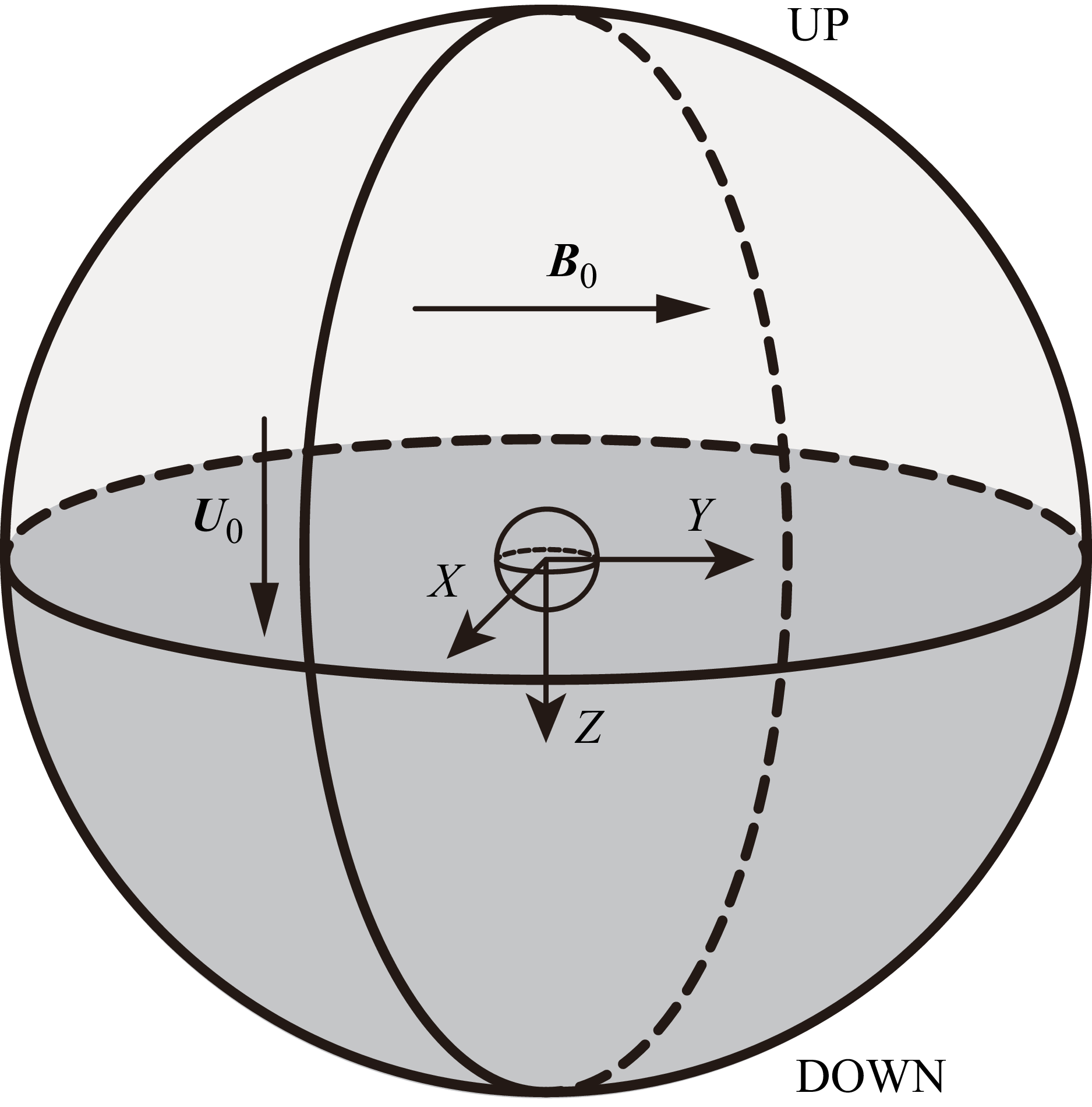
The flow configuration around the moving sphere and relevant geometrical parameters are presented in figure 1. The movement of the sphere is limited to the positive Zaxis through the simulation. The simulation of this paper is under the assumption of infinite domain and mainly investigates the flow around the sphere, so any interactions between the wake and the boundaries are not considered. Therefore, the pressure and velocity on the down surface are set as far-field conditions with a zero pressure gradient and zero velocity. On the up surface, a fixed pressure and zero-gradient velocity are imposed for numerical convenience. The no-slip boundary condition is applied on the sphere surface.
Schematic diagram of the computational domain and configurations. The upper hemispherical surface defines the boundary UP (light grey part), while the lower hemispherical surface represents the boundary DOWN (dark grey part). A uniform magnetic field
 $\boldsymbol{{B}}_0$
is applied along the positive Y axis, and the sphere initially moves with a constant velocity
 $\boldsymbol{{U}}_0$
along the positive Z axis before undergoing an impulsive stop.

To resolve the Hartmann layer correctly and balance the computational time, the finest mesh is adopted at the surface of the sphere. Considering the mesh orthogonality, the computational domain is designed to a spherical area and a O-type mesh is adopted here. Generally speaking, the flow around a sphere is extremely important due to the existence of a boundary layer. The thickness of the boundary layer depends on the Reynolds number in the absence of a magnetic field. While imposing a magnetic field, the thickness of the Hartmann layer has to be considered, which depends mainly on the Hartmann number
 $ \textit{Ha} = (N {\textit{Re}}_{\!D})^{1/2}$
. The parameter ranges investigated in this paper are basically
 $60\leqslant {\textit{Re}}_{\!D} \leqslant 300$
and
 $ 0\leqslant N \leqslant 10$
, which corresponds to
 $0\leqslant \textit{Ha}\leqslant 54.8$
. Nevertheless, in order to explore the influence of magnetic field on the wake structure and particle dynamics at high Reynolds numbers, simulations with
 ${\textit{Re}}_{\!D}=1000$
for
 $ 0\leqslant N \leqslant 10$
were included in this study, which corresponds to
 $0\leqslant \textit{Ha}\leqslant 100$
. Utilising experience from our previous studies (Pan et al. Reference Pan, Zhang and Ni2019b
; Cai et al. Reference Cai, Pan and Ni2022), the thickness of the first layer on the sphere surface is set to
 $\delta _{\textit{min}} = 0.005D$
at
 ${\textit{Re}}_{\!D} \leqslant 300$
and
 $\delta _{\textit{min}} = 0.005D$
and
 $\delta _{\textit{min}} = 0.0025D$
at
 ${Re_D}=1000$
for the grid independence verification. The mesh spacing of all other meshes is then increased with an appropriate ratio of less than 1.1 far away from the sphere surface. Consequently, there are four to five grid layers to solve the strong shear layer. Five meshes are detailedly used to examine the grid independence for ensuring the accuracy of simulations in this paper. The extreme parameters
 ${\textit{Re}}_{\!D}=300$
and
 $N=10$
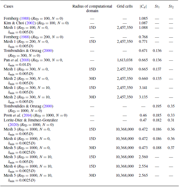
are tested here. The drag coefficient and frequency of vortex shedding at the fully developed stage of the wake are used to examine results of the test. Exact configurations are presented in table 1. In addition, for ease of data description, a new dimensionless variable
 $t^*=t-t_{\textit{stop}}$
is introduced here, where
 $t_{\textit{stop}}$
is the dimensionless time of the sphere’s impulsive stop. As observed from the moving reference frame attached to the moving sphere, there is essentially no difference between the drag of flow past a fixed sphere and the drag of a sphere moving in a quasi-static fluid. So the drag coefficient is compared with previous results of flow past a fixed sphere in table 1. Besides, the power spectrum of the streamwise velocity component for a point in the wake is plotted in figure 2(b) for comparing with previous fixed sphere results. The statistical primary frequency of flow past a sphere at
 ${\textit{Re}}_{\!D}=1000$
without a magnetic field and the second higher frequency are both in agreement with several previous studies, as presented in table 1. Based on the comparison results, mesh 1 for
 ${\textit{Re}}_{\!D} \leqslant 300$
and mesh 4 for
 ${\textit{Re}}_{\!D}=1000$
are selected for subsequent simulations, where the meshes are confirmed to sufficiently resolve the flow field.
Grid independence test and validation. Here
 $|C_d|$
is recorded as the average value after the flow reaches a statistical steady state;
 $St_1$
and
 $St_2$
are the primary frequency and the frequency relevant with the Kelvin–Helmholtz instability (Tomboulides & Orszag Reference Tomboulides and Orszag2000), respectively. The frequencies are both non-dimensionalised by
 $U_0/D$
.

The grid resolution test. (a) Close-up view of the mesh around the sphere. (b) Power spectrum of the streamwise velocity component for a point located 5D downstream of the sphere in the wake at
 ${\textit{Re}}_{\!D}=1000$
without a magnetic field.

3. Flow around a sphere following an impulsive stop
The flow around a sphere undergoing an impulsive stop under the influence of a magnetic field differs significantly from that observed in conventional hydrodynamic flows past a fixed sphere. Due to the characteristics of MHD flows, the orientation of the magnetic field relative to the primary flow direction plays a critical role in forming the flow structure. This section examines the flow structures around a sphere following an impulsive stop in the presence of a uniform transverse magnetic field. In all cases, the magnetic field is imposed from the beginning of the simulation and the flow is first computed to a fully developed state prior to the sphere’s impulsive stop. The parameter range investigated here is
 $60 \leqslant {\textit{Re}}_{\!D} \leqslant 300$
and
 ${\textit{Re}}_{\!D} = 1000$
with
 $0 \leqslant N \leqslant 10$
.
3.1. Vortex structures at
 $60 \leqslant {\textit{Re}}_{\!D} \leqslant 300$
with
$0 \leqslant N \leqslant 10$


The wake generated by the moving sphere continues to propagate downstream after the sphere undergoes an impulsive stop, forming a more complex vortex system due to the presence of the stationary sphere. Vortices appear in the sphere wake, exhibiting an axisymmetric and steady behaviour at
 $20 \lt {\textit{Re}}_{\!D} \lt 210$
, a steady planar symmetric behaviour between
 $210 \lt {\textit{Re}}_{\!D} \lt 270$
and an unsteady planar symmetric behaviour at
 ${\textit{Re}}_{\!D} \gt 270$
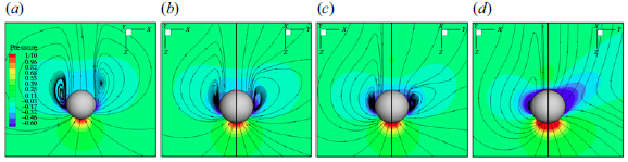
(Johnson & Patel Reference Johnson and Patel1999). The primary flow after the impulsive stop is aligned with the direction of the sphere’s prior motion, namely the positive Z axis, so the negative Z zone is referred to as the upstream region and the positive Z zone is referred to as downstream, as shown in figure 3(a). At the moment of the impulsive stop, the vortex closest to the sphere, defined as the primary vortex, interacts immediately with the sphere. At short time scales after the impulsive stop, the primary vortex still locates on the upstream side of the sphere and pulls streamlines away from the sphere surface, promoting the development of the recirculation zone, as shown in figure 3(b). At long time scales, when
 ${\textit{Re}}_{\!D}$
is large enough, the primary vortex propagates to the downstream side, as shown in figure 3(c). The streamlines are pushed close to the sphere surface due to the primary vortex located on the downstream side. The influence of the primary vortex on the recirculation gradually shifts from enhancement to suppression as it moves from the upstream to downstream side. Moreover, the presence of the primary vortex downstream facilitates the shedding of the vortex in the recirculation zone due to the induced velocity. Meanwhile, the vortices gradually move away from the sphere surface owing to inertia and the self-induced velocity of the vortex ring.
The unsteady nature of the flow after the stop leads to a time-dependent evolution of the wake structures. A fixed dimensionless time of
 $t^* = 6$
is used to characterise and compare the flow features in the following analysis. At this moment, the primary vortex propagates downstream across most Reynolds numbers and interaction parameters. To elucidate the influence of a transverse magnetic field, the flow structures at
 $N=0$
are first discussed here. The instantaneous streamlines, the vortex structures identified by the Q-criterion and the corresponding skin friction lines on the downstream surface of the sphere are shown in figure 4. Lighthill (Reference Lighthill1963) pointed out that skin friction lines converge at separation regions in three-dimensional flow, providing a clear representation of flow traces around the sphere, enabling a more effective analysis of flow structures. At
 ${\textit{Re}}_{\!D}=100$
, no vortex ring forms downstream and the skin friction lines converge at a single central point. This indicates that the flow prior to the impulsive stop lacks sufficient energy to generate a recirculation zone, instead merely following the sphere surface downstream as presented in the streamlines plot. At
 ${\textit{Re}}_{\!D}=200$
,
 $250$
and
 $300$
, a downstream vortex ring is clearly observed, which is actually the primary vortex propagating downstream. The corresponding skin friction lines form a closed convergence line, indicating the presence of a recirculation zone near the downstream side of the sphere. Moreover, the vortex system exhibits axisymmetry at
 ${\textit{Re}}_{\!D}=100$
and
 $200$
, but transitions to planar symmetry at
 ${\textit{Re}}_{\!D}=250$
and
 $300$
, which is consistent with the flow past a stationary sphere. As a result, the vorticity on the symmetry plane becomes asymmetric between the two sides of the sphere and exhibits alternating dominance at higher Reynolds numbers. This asymmetry leads to unequal recirculation strengths on both sides, causing the divergence point to deviate from the centre point. At
 ${\textit{Re}}_{\!D}=300$
, the asymmetry becomes more pronounced, resulting in skin friction lines that converge into a non-circular closed line, in contrast to the nearly circular convergence line at
 ${\textit{Re}}_{\!D}=200$
and
 $250$
. Nevertheless, the symmetry of the skin friction lines remains consistent with that of the vortex ring.
Schematic illustrating the flow evolution process following the impulsive stop of the sphere. The upstream and downstream regions are demarcated by the plane passing through the sphere centre and oriented perpendicular to the sphere motion direction. The vortex structures might not be symmetrical at higher Reynolds numbers. The sphere velocity before the impulsive stop is from top to bottom. (a) Before the impulsive stop; (b) short time scales after the impulsive stop; (c) long time scales after the impulsive stop.

Vortex structures and corresponding skin friction lines on the downstream surface of the sphere without a magnetic field for various
 ${\textit{Re}}_{\!D}$
. The top row shows instantaneous streamlines on the symmetry plane. The middle row presents vortex structures identified by the Q-criterion and the bottom row shows skin friction lines. All plots are from the data at
 $t^*=6$
. Results are shown for (a)
 ${\textit{Re}}_{\!D}=100$
, (b)
 ${\textit{Re}}_{\!D}=200$
, (c)
 ${\textit{Re}}_{\!D}=250$
, (d)
 ${\textit{Re}}_{\!D}=300$
.

The wake of the sphere influenced by a transverse magnetic field with different strengths can be categorised into three main states: the steady double-plane symmetric state, the steady plane symmetric state and the unsteady plane symmetric state (Pan et al. Reference Pan, Zhang and Ni2019b
). Due to the different initial states at the instant the sphere impulsively stops, various vortex structures are generated and developed under the influence of a magnetic field with various strengths. Pan et al. (Reference Pan, Zhang and Ni2018, Reference Pan, Zhang and Ni2019b
) reported a ‘reversion phenomenon’ in the study of wake structure behind a sphere, which means that the topological structure with a higher
 ${\textit{Re}}_{\!D}$
and a higher
 $N$
is similar to the case with lower
 ${\textit{Re}}_{\!D}$
and
 $N$
. Furthermore, the magnetic field typically counteracts the inertia effects of the fluid, exerting a stabilising influence at lower Reynolds numbers and interaction parameters (Zheng, Pan & Ni Reference Zheng, Pan and Ni2023). Consequently, within the range
 $60\leqslant {\textit{Re}}_{\!D}\leqslant 300$
and
 $0\leqslant N\leqslant 10$
, the flow behaviour at
 ${\textit{Re}}_{\!D}=300$
with varying interaction parameters may exhibit greater complexity. Therefore, the cases at
 ${\textit{Re}}_{\!D}=300$
for
 $0\leqslant N\leqslant 10$
are discussed first. For comparison, the instantaneous streamlines at the fully developed state with different
 $N$
are provided in Appendix A. The vortex structures and corresponding skin friction lines on the downstream surface of the sphere at
 ${\textit{Re}}_{\!D}=300$
with corresponding
 $N$
are presented in figure 5. At
 $N=0.05$
, the vortex near the sphere propagates downstream and detaches, forming a primary vortex structure identified by the Q-criterion. With increasing
 $N$
, the formation of the primary vortex structure becomes increasingly incomplete and is eventually confined to the upstream region. Consequently, four distinct flow regimes emerge, each associated with a characteristic topology of skin friction lines, as shown in the bottom row.
Vortex structures and corresponding skin friction lines on the downstream surface of the sphere at
 ${\textit{Re}}_{\!D}=300$
with various
 $N$
at
 $t^* = 6$
. The top row presents vortex structures identified by the Q-criterion and the bottom row shows skin friction lines. Results are shown for (a)
 $N=0.05$
, (b)
 $N=0.2$
, (c)
 $N=0.5$
, (d)
 $N=4$
.

Skin friction lines on the downstream surface of the sphere and azimuthal vorticity contours at
 ${\textit{Re}}_{\!D}=300$
with
 $N=0.01$
for different impulsive stop instants within a vortex-shedding period. Results are shown for (a,b)
 $t_{\textit{stop}}=0T$
and (c,d)
 $t_{\textit{stop}}=1/2T$
. Azimuthal vorticity contours are shown on the symmetry plane normal to the Yaxis. From left to right is the positive X direction.

At
 ${\textit{Re}}_{\!D}=300$
and
 $N=0.05$
, the magnetic field is relatively weak, so the flow around the sphere resembles that in the absence of a magnetic field as shown in figures 4(d) and 5(a). Periodic vortex shedding occurs for
 $t^*\lt 0$
and a primary vortex ring forms as the wake continues moving downstream and interacts with the sphere. When the sphere is impulsively stopped at different times within the shedding period, slight variations in the skin friction lines arise. Figure 6 compares the flow fields at two representative stop times,
 $t_{\textit{stop}} = 0T$
and
 $t_{\textit{stop}} = 1/2T$
, where
 $T$
is the vortex-shedding period prior to the stop. A prominent accompanying vortex appears near the sphere for
 $t_{\textit{stop}}=1/2T$
, which corresponds to the vortex shed from the sphere prior to the impulsive stop. For
 $t_{\textit{stop}}=0T$
, a weak accompanying vortex also emerges on the upstream side of the sphere, while it is much weaker as it had not yet been shed completely prior to the impulsive stop. However, a more pronounced vortex is observed farther away from the sphere. This distant vortex gradually moves closer to the sphere due to inertial effects while simultaneously dissipating, as indicated by the azimuthal vorticity contour in figure 6(b). Differences in the skin friction lines are also observed between the two impulsive stop instances, as shown in figure 6(a,c). When
 $t_{\textit{stop}} = 1/2T$
, a closed circular convergence line forms on the downstream surface of the sphere, indicating a recirculation zone extending continuously in the azimuthal direction. However, at
 $t_{\textit{stop}} = 0T$
, the convergence line of the skin friction lines is not closed, suggesting the absence of recirculation on the right-hand side, as shown in figure 6(a). As illustrated in figure 3, the upstream vortex pulls streamlines away from the sphere, promoting recirculation, while the downstream vortex pushes streamlines toward the sphere, suppressing recirculation. In both cases, the wake retains sufficient residual energy to sustain recirculation after the impulsive stop. For
 $t_{\textit{stop}} = 0T$
, the primary vortex on the right-hand side retains enough energy to suppress recirculation, preventing the formation of a closed convergence line. However, for
 $t_{\textit{stop}} = 1/2T$
, a strong upstream accompanying vortex closer to the sphere facilitates the formation of recirculation, counteracting the suppression from the downstream primary vortex. As a result, a convergence line also forms on the right-hand side, completing a closed convergence loop, as shown in figure 6(d). Although the skin friction lines differ slightly between the two cases, the underlying vortex structures remain fundamentally similar. Accordingly, both cases are classified as model V in figure 8.
Effect of a directionally anisotropic Lorentz force damping on wake structural dynamics. (a) Isosurface of azimuthal vorticity at
 ${\textit{Re}}_{\!D}=300$
,
 $N=0.2$
. (b) Distribution of the main current lines around the sphere. (c) The Z component of the Lorentz force contour in a section 0.5
 $D$
away from the sphere centre. The circle of the black solid line represents the vertical projection of the sphere along the Zaxis on the plane. The direction perpendicular to the paper and outward is the positive direction of the Z axis.

At
 ${\textit{Re}}_{\!D} = 300$
and
 $N = 0.2$
, the anisotropic influence of the transverse magnetic field on the vortex structure gradually emerges, promoting a transition toward a steady wake characterised by double-plane symmetry in the fully developed stage. At
 $t^*\lt 0$
, vortex shedding is entirely suppressed, resulting in a flow field that is perfectly symmetric on the plane perpendicular to the magnetic field. At
 $t^*\gt 0$
, the wake propagates downstream and develops into a primary vortex ring, as illustrated in figure 5(b). In contrast to the streamwise magnetic field configuration, a transverse magnetic field disrupts the circumferential symmetry of the primary vortex. This symmetry breaking originates from the misalignment between the velocity vector of the vortex ring and the direction of the applied transverse magnetic field. An isolated view of the primary vortex from the negative Z-axis perspective, as presented in figure 7(a). The distinctive vortex ring size results from spatial variations in the Lorentz force across different flow regions. To elucidate the Lorentz force distribution, the spatial distribution of current lines around the stopped sphere at
 $t^*=6$
is presented in figure 7(b). According to Ohm’s law (2.3), the electric current comprises two components: one induced by electromotive effects and the other arising from electrostatic potential. The former is generated by the motion of conducting fluid within a magnetic field, while the latter results from electric potential gradients. A competition between these two components determines the local distribution of electric current within the computational domain.
In the present flow configuration, the sphere moves with a constant velocity for
 $t^*\lt 0$
, causing the fluid near the sphere to flow downstream, while the fluid farther away remains nearly stationary. As a result, electromotive effects dominate the electric current in the vicinity of the sphere, whereas electrostatic potential contributions prevail in the region far from the sphere. The sphere moves at a constant velocity along the positive Z axis for
 $t^*\lt 0$
, inducing a downstream fluid motion with velocity vectors predominantly aligned in the same direction for
 $t^*\gt 0$
. Consequently, the flow interacts with the applied magnetic field oriented along the positive Y axis, generating electric currents along the negative X axis near the sphere, in accordance with Ohm’s law. In the region far from the sphere, the flow velocity is significantly weaker. Therefore, the current direction is governed by the electric potential induced by the currents near the sphere, resulting in a net current flowing along the positive Xaxis. Meanwhile, due to the charge conservation law and the electrically insulating condition of the sphere, current lines are closed and bend along the sphere surface, as shown in figure 7(b).
A simple map of skin friction line patterns on the downstream surface of an impulsively stopped sphere in the plane
 $\{N,{\textit{Re}}_{\!D}\}$
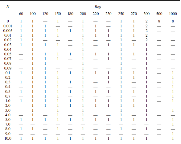
. The direction of the magnetic field is transverse with the motion direction of a sphere. Marks of various shapes represent calculated data points, of which only a subset is shown for clarity. A summary of the simulation cases is provided in table 2 in Appendix B. The patterns are divided into five regimes labelled I, II, III, IV and V, corresponding to five schematic diagram models on the right-hand side, respectively. Model I: one straight convergent line; model II: one convergent point; model III: one circular convergent line with one divergent point located at the centre; model IV: one circular convergent line with two divergent points located at two sides of the centre; model V: one circular convergent line with one off-centre convergent point. Here
 $\circ$
and
 $\square$
respectively represent the convergence point and the divergence point.

The currents, interacting with the applied magnetic field oriented along the positive Y axis, generate Lorentz forces directed along the positive Z axis in the region far from the sphere and along the negative Zaxis near the sphere, as illustrated in figure 7(c). The Lorentz forces suppress the flow along the positive Zaxis near the sphere, and again damp the flow in the upper and lower regions farther away. As a result, the vorticity near the Y–Z plane is more strongly suppressed than that near the X–Z plane. Accordingly, the isosurface of azimuthal vorticity becomes progressively thinner from the Y–Z plane to the X–Z plane along the circumferential direction, as shown in figure 7(a). Moreover, the wake retains sufficient energy to form recirculation around the sphere surface, resulting in a closed circular convergence line in the skin friction lines, as presented in figure 5(b). The stronger primary vortex on the downstream side of the sphere along the X direction pushes the streamline closer to the sphere surface, ultimately delaying flow separation on the X–Z plane. Consequently, the convergence line of skin friction lines in figure 5(b) develops an elliptic shape with its major axis aligned along the Y direction. Nevertheless, a circular convergence line and a divergence point appear in the skin friction lines in this class of flow pattern, which is categorised as model III in figure 8.
At
 ${\textit{Re}}_{\!D}=300$
and
 $N=0.5$
, the difference in the damping effect of the transverse magnetic field between the regions near the Y–Z plane and the X–Z plane enhances. The wake still contains enough energy to form the recirculation zone downstream. However, at
 $t^*=6$
, the primary recirculations appear on both sides and have not yet developed to be adjacent. After passing the two primary recirculation zones, the flow remains closely attached to the sphere surface. When the streamlines from both sides meet near the downstream centre, the fluid tends to move along the magnetic field direction (Yaxis) because the damping in other directions is stronger. Ultimately, this seems like the separation of a single divergence point into two, and the line connecting them is perpendicular to the magnetic field, as shown in figure 5(c), which is concluded as model IV in figure 8. With further increases in magnetic field strength, the flow perpendicular to the magnetic field direction weakens dramatically, becoming insufficient to generate a recirculation zone. Consequently, the closed convergence lines in the skin friction line diagram vanish, transforming into a single convergence line driven primarily by the flow parallel to the magnetic field direction. Although the flow intensity in the Y-axis direction remains relatively high, the transverse magnetic field causes the flow near the bottom of the sphere to align parallel to the magnetic field, preventing the occurrence of recirculation. As a result, the skin friction lines form a straight line crossed by the centre at
 ${\textit{Re}}_{\!D}=300$
with
 $N=4$
, as shown in figure 5(d), which is concluded as model I in figure 8. Moreover, the straight and convergent skin friction line is perpendicular to the direction of the transverse magnetic field due to the preferred orientation of the vortex symmetry plane at
 $t^*\lt 0$
, reported by Pan et al. (Reference Pan, Zhang and Ni2019b
).
At lower Reynolds numbers, the wake lacks sufficient energy to sustain recirculation, primarily due to the limited residual energy from the wake prior to the impulsive stop. Meanwhile, when the transverse magnetic field is relatively weak, the anisotropy damping effect is not pronounced. Therefore, the skin friction lines exhibit nearly axisymmetric patterns and converge at a centre point on the sphere surface, resembling the topological structure observed in the absence of a magnetic field at
 ${\textit{Re}}_{\!D}=100$
. This flow pattern can be categorised as model II in figure 8. Moreover, as the interaction parameters varies, flow patterns corresponding to models III, IV and V can also be observed for
 $150 \leqslant {\textit{Re}}_{\!D} \leqslant 300$
. Due to the different initial states mentioned above before the impulsive stop of the sphere and the influence of the transverse magnetic field, there are a total of five primary flow types at
 $60 \leqslant {\textit{Re}}_{\!D} \leqslant 300$
with
 $0 \leqslant N \leqslant 10$
, as shown in the skin friction lines diagram in figure 8. After a series of numerical simulations for nearly 200 cases, flow structures following the impulsive stop of the sphere are categorised into five regimes in the
 $\{N,{\textit{Re}}_{\!D}\}$
phase plot as shown in figure 8, based on the diagrams of skin friction lines. In the phase plot, marks of various shapes represent calculated data points, of which only a subset is shown for clarity. The cases summary is provided in table 2 in Appendix B.
3.2. Vortex structures around an impulsively stopped sphere at
${\textit{Re}}_{\!D}=1000$

Most previous studies have focused on
 ${\textit{Re}}_{\!D}\leqslant 300$
, whereas cases at slightly higher Reynolds numbers can exhibit more complex flow structures. For example, Tomboulides & Orszag (Reference Tomboulides and Orszag2000) reported that the wake at
 ${\textit{Re}}_{\!D}=1000$
becomes weakly turbulent due to the presence of the Kelvin–Helmholtz instability. To explore this regime, the case of
 ${\textit{Re}}_{\!D}=1000$
with
 $0\leqslant N\leqslant 10$
is investigated in this subsection. In all cases, the sphere is brought to a impulsive stop after travelling a sufficient distance to reach a fully developed state. When
 $N\gt 0$
, the imposed magnetic field is present from the beginning of the simulation.
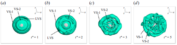
Temporal evolution of vortex structures visualised using the Q-criterion (
 $Q_{\textit{criterion}}=1$
) at
 ${\textit{Re}}_{\!D}=1000$
without a magnetic field. Results are shown for (a)
 $t^*=-12$
, (b)
 $t^*=0$
, (c)
 $t^*=1$
, (d)
 $t^*=5$
.

Vortex structures visualised using the Q-criterion (
 $Q_{\textit{criterion}}=1$
) at
 ${\textit{Re}}_{\!D}=1000$
with
 $N=0.3$
at
 $t^*=6$
. Panels (a) and (b) represent the views at the symmetry plane perpendicular to the Yaxis and the X axis, respectively.

In the absence of a magnetic field, complex wake structures comprising small-scale vortices due to the Kelvin–Helmholtz instability are observed at
 $t^* \lt 0$
, as shown in figure 9. A prominent vortex-shedding period is present, indicating the formation of fundamental vortex structures in the wake. Meanwhile, as shown in figure 2(b), a secondary and slightly pronounced vortex-shedding frequency is also detected, suggesting the presence of numerous secondary induced vortices appear among the primary vortices as illustrated in figure 9(a). Compared with the
 ${\textit{Re}}_{\!D}=300$
cases, more complex vortex structures are revealed at
 ${\textit{Re}}_{\!D}=1000$
when visualised using the same Q-criterion threshold, indicating the generation of a stronger wake. Following the impulsive stop (
 $t^* \gt 0$
), the residual kinetic energy remains sufficiently large for the downstream vorticity to detach from the sphere surface, forming a sequence of vortex structures, including a leading vortex structure (LVS), a first vortex structure (VS-1) and a second vortex structure (VS-2). Details of their formation and interaction are provided in Appendix A. During the wake evolution, a primary vortex structure develops downstream and a series of accompanying vortices interact with the sphere simultaneously, as shown in figure 9(d). The overall interaction pattern is broadly similar to that observed at
 ${\textit{Re}}_{\!D}=300$
, except that numerous small-scale vortices coexist with the fundamental vortex structures.
With the application of a transverse magnetic field, the wake structure before the impulsive stop tends to develop a double-plane symmetric state as
 $N$
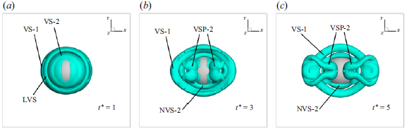
increases. As demonstrated in figure 7, the Lorentz force induces anisotropy, enhancing vorticity generation in the X–Z plane and confining vortex shedding within this plane, unlike the helical shedding without a magnetic field. After the stop, a primary vortex forms and, under the anisotropic magnetic influence, an additional vortex-pair structure (VSP-2) develops as shown in figure 10, arising from the combined effects of VS-1 induction and the residual wake energy. A detailed visualisation of these vortex structures is provided in Appendix A. Due to the anisotropic damping, vortices aligned with the magnetic field exhibit greater intensity, particularly near the Y–Z plane. The downstream vortex structure VS-1 suppresses recirculation, causing the convergence line of skin friction lines near the X–Z plane to shift closer to the central point, indicating a delayed onset of recirculation. This produces a gourd-like closed convergent line, as presented in figure 11(a), deviating from circular or elliptical shapes but consistent with model III. Similar to cases with lower Reynolds numbers, as
 $N$
increases further, the vortex-shedding period approaches infinity, indicating the emergence of a completely steady wake behind the sphere. Moreover, the kinetic energy of the flow around the sphere decays progressively, eventually becoming insufficient to sustain a recirculation zone. As a consequence, the skin friction lines exhibit the characteristics described in model I, featuring only a straight convergent line perpendicular to the magnetic field direction as presented in figure 11(c). Further details about the influence of the transverse magnetic field on the wake evolution are provided in Appendix A. With the increment of
 $N$
at
 ${\textit{Re}}_{\!D}=1000$
, the pattern of skin friction lines undergoes a sequence of transitions, model III
 $\to$
IV
 $\to$
I, which is similar to cases at
 ${\textit{Re}}_{\!D}=300$
. This consistent transition pathway reaffirms the presence of the ‘reversion phenomenon’.
Skin friction lines on the downstream surface of the sphere at
 $t^*=6$
for
 ${\textit{Re}}_{\!D}=1000$
with various interaction parameters. Results are shown for (a)
 $N=0.3$
, (b)
 $N=0.9$
, (c)
 $N=5$
.

4. Decay of the drag coefficient following an impulsive stop
The hydrodynamic behaviour of a sphere in an electrically conducting fluid is influenced by MHD effects, where the applied magnetic field interacts with the motion fluid to induce the Lorentz force that modifies the flow field and consequently affects the sphere’s dynamics. The influence of the surrounding fluid modified by MHD effects on the sphere’s dynamics can be characterised conventionally using a drag coefficient to quantify the resultant force on the sphere. Besides, the drag at
 $t^*\lt 0$
is different within the different parameters. Therefore, in this section a normalised drag coefficient, defined as
 \begin{align} C_d^*=\frac {C_{d,{t^*\gt 0}}}{\lvert {C_{d,{t^*\lt 0}}\rvert }}, \end{align}
is introduced to investigate the force acting on the sphere for
 $t^*\gt 0$
under a transverse magnetic field. Here,
 $C_d$
represents the dimensionless drag coefficient, defined as
 \begin{align} C_d = \frac {F_d}{\dfrac {1}{2}\rho {U_0}^2 A}, \end{align}
where
 $F_d$
is the drag force,
 $\rho$
is the fluid density,
 $U_0$
is the constant velocity of the sphere for
 $t^*\lt 0$
and
 $A$
is the projected area of the sphere along the
 $U_0$
direction. The term
 $\lvert C_{d,{t^*\lt 0}} \rvert$
denotes the average drag coefficient for
 $t^*\lt 0$
after the flow around the sphere reaching a fully developed state.
While previous studies have established drag decay laws mainly for low-Reynolds-number regimes, extending these results to higher Reynolds numbers and magnetic field conditions remains challenging due to the complexity of the unsteady flow. Based on the physical process described in the preceding section and the physical interpretation of the drag formulation components, a drag decomposition framework is constructed in this section. This framework enables the derivation of drag decay scaling laws that remain valid beyond the Stokes regime. The subsequent subsections present the inspiration, examination and extension of this framework.
4.1. Inspiration in the Stokes flow regime
To better understand the influence of vortex evolution on drag following the impulsive stop of a sphere, insight is first drawn from the classical Stokes flow. In the classical first Stokes problem, an infinite plate impulsively starts from rest and moves at a constant velocity parallel to its surface. The velocity profile as a function of time
 $t$
and the wall-normal coordinate
 $z$
can be obtained by solving the governing equation using the method of the separation of variables. Analogously, for an infinite plate that impulsively stops from a constant velocity, the velocity profile
 $u(z, t)$
can be derived as
 \begin{equation} u(z, t) = u_0 {\textit{erf}}(\eta ) = u_0 \frac {2}{\sqrt {\pi }} \int _{0}^{\eta } {\rm e}^{-\lambda ^2} \, {\rm d}\lambda ,\end{equation}
where the dimensionless variable
 $\eta = {z}/{2\sqrt {\nu t}}$
and
 $u_0$
is the velocity of the plate prior to the stop. The shear force per unit area acting on the plate can be expressed as
 \begin{equation} f_{\textit{plate}} = \rho \nu \left . \frac {\partial u}{\partial z} \right |_{z=0} = \frac {\rho u_0 \sqrt {\nu }}{\sqrt {\pi t}}. \end{equation}
Based on the fluid density
 $\rho$
and the initial plate velocity
 $u_0$
, the force can be non-dimensionalised into a force coefficient defined as
 \begin{equation} C_{d, {\textit{plate}}} = \frac {f_{\textit{plate}}}{\frac {1}{2} \rho u_0^2} = \frac {2}{\sqrt {\pi }}\frac {\nu }{u_0 \sqrt {\nu t}} = \frac {2}{\sqrt {\pi }}\frac {1}{{\textit{Re}}} ,\end{equation}
where
 ${\textit{Re}}$
is the Reynolds number based the characteristic length scale
 $\sqrt {\nu t}$
. Following the impulsive stop of the plate, vorticity is generated at the surface and diffuses outward in the wall-normal direction, forming a thin vorticity-concentrated boundary layer whose thickness grows as
 $\sqrt {\nu t}$
. This diffusive length scale characterises the unsteady flow field and naturally serves as the basis for constructing a time-dependent drag scaling law.
Inspired by the classical first Stokes problem and (4.5), the temporal evolution of the drag coefficient following an impulsive stop can be inferred by adopting the vorticity diffusion scale,
 $\sqrt {\nu t^*}$
, as the characteristic length. In the Stokes flow regime the drag coefficient of a sphere is given by
 $ {24}/{{\textit{Re}}_{\!D}}$
. At short time scales following the impulsive stop of the sphere, the vorticity is generated on the sphere surface and diffuses outward. By substituting the vorticity diffusion length scale into the drag expression after the impulsive stop, a temporal scaling of
 $C_d^{\textit{Stokes}} \sim {{\textit{Re}}}^{-1} \sim {t^*}^{-1/2}$
is obtained, in agreement with the classical result rigorously derived from the Stokes equations by Basset (Reference Basset1888). This scaling behaviour is further validated by the present numerical simulation at
 ${\textit{Re}}_{\!D}=0.1$
as shown in figure 12, where the temporal evolution of the drag coefficient agrees well with both the present scaling prediction and the analytical solution in Basset (Reference Basset1888), confirming the validity of the proposed characteristic length scale and the underlying assumptions of the scaling analysis. Moreover, the flow around the sphere retains the characteristics as Stokes flow at both short time scales and long time scales following the impulsive stop, as shown in figure 12(b,c). However, the drag decay exhibits two distinct scaling laws:
 ${t^*}^{-1/2}$
at short time scales and
 ${t^*}^{-1}$
at long time scales. The former can be predicted well by the present scaling analysis, whereas the latter has been derived based on the global mass and momentum conservation principles (Lawrence & Mei Reference Lawrence and Mei1995). In Lawrence & Mei (Reference Lawrence and Mei1995) the flow is assumed to be fully developed both before and after the impulsive stop, and the
 ${t^*}^{-1}$
decay law is obtained by analysing the decay of the characteristic velocity at long time scales.
Verification at low Reynolds numbers
 ${\textit{Re}}_{\!D}=0.1$
. (a) The time history of the normalised drag coefficient; (b) instantaneous streamlines on the symmetry plane at short time scales; (c) instantaneous streamlines on the symmetry plane at long time scales.

4.2. Extension to inertia and MHD damping effects
The previously discussed scaling law, derived from the Stokes flow, is valid only in the low-Reynolds-number regime where the inertial effect is negligible. However, as the Reynolds number increases, inertial effects become significant and the presence of a transverse magnetic field introduces additional damping on the flow through the Lorentz force. To extend the drag decay analysis to this more general regime, appropriate corrections must be incorporated. The corrections can be systematically derived within the scaling analysis framework, which is inspired in the Stokes regime through substituting the characteristic length scale in drag coefficient expressions.
The drag on a sphere has been extensively studied, with the inertia correction introduced to the classical Stokes drag at high Reynolds numbers. At low but finite Reynolds numbers, Oseen’s theory refines the classical Stokes drag by incorporating the convective inertia correction, yielding the Oseen drag
 ${24}/{{\textit{Re}}_{\!D}}(1 +({3}/{16}) {\textit{Re}}_{\!D})$
. The second term in this expression represents the first-order inertial correction and is valid within the low-Reynolds-numbers regime. At higher Reynolds numbers, the semi-empirical formula
 $C_d = {24}/{{\textit{Re}}_{\!D}}(1 + 0.15{\textit{Re}}_{\!D}^{0.687})$
is commonly used across a wide range of Reynolds numbers (Clift, Grace & Weber Reference Clift, Grace and Weber2005). Analogous to the Oseen drag, the second term can also be considered as a correction part, introducing inertia effects at high Reynolds numbers. Consequently, the sphere drag can be considered as comprising two parts: the Stokes part
 $C_d^{\textit{Stokes}} \sim {{\textit{Re}}^{-1}}$
and a correction part
 $C_d^{\textit{correction}} \sim {{\textit{Re}}^{-1/3}}$
. The Stokes part can be derived as
 $C_d^{\textit{Stokes}} \sim {{t^*}^{-1/2}}$
, as illustrated in § 4.1. For the correction part, we need to consider two components: the inertia effect and MHD effect. At high Reynolds numbers, convection induced by the inertia effect becomes increasingly significant, indicated by the formation and propagation of vortex structures, which are both relevant to the vorticity diffusion scale. Inspired by the Stokes part in § 4.1, the vorticity diffusion distance is adopted as the characteristic length scale of the inertia correction component, deriving
 $C_d^{\textit{inertia}} \sim {({t^*}^{1/2})^{-1/3}} \sim {t^*}^{-1/6}$
.
Drag decomposition model. The drag decay following an impulsive stop of a sphere is decomposed into three contributions: the original Stokes effect, an inertia correction and a MHD correction. Based on the vorticity diffusion scale and the drag coefficient formulation, the temporal scalings associated with each contribution are derived and summarised here.

Furthermore, the scaling law analysis of drag is extended to account for the presence of a transverse magnetic field here. Due to the increasingly significant dissipation induced by the transverse magnetic field as the interaction parameter increases, the vorticity magnitude decays over time. This decay can be quantitatively characterised by the decay of the angular momentum
 $\varGamma \sim {t^*}^{-1/2}$
(Davidson Reference Davidson2001). Since the viscous forces scale proportionally with angular momentum and appear in the denominator part of
 ${\textit{Re}}$
, the correction to the drag coefficient induced by the MHD effect can be expressed as
 $C_d^{\textit{MHD}} \sim {{\textit{Re}}^{-1/3}} \sim ({\textit{inertia}\, \textit{force}}/{{\textit{viscous}\, \textit{force}}})^{-1/3} \sim ( {1}/{{t^*}^{-1/2}})^{-1/3} \sim {t^*}^{-1/6}$
. The Stokes effect, as originally derived from theoretical analyses (Basset Reference Basset1888; Lawrence & Mei Reference Lawrence and Mei1995), along with the present extensions incorporating for inertia and MHD effects, are schematically illustrated and summarised in figure 13. Notably, although partial flow separation occurs after the impulsive stop, the sphere remains predominantly enveloped by the surrounding flow, representing the baseline Stokes contribution to the drag. The inertia effect and the MHD damping effect both influence the enveloped flow, further influencing the drag decay. Therefore, the inertia and MHD corrections are superimposed on the baseline Stokes flow, and the coupled decay law is obtained through a multiplicative combination of these effects rather than a simple additive relation. The drag coefficient for
 $t^*\gt 0$
is influenced by these three components in different ways, depending on the Reynolds number, the interaction parameter and the characteristic time scale.
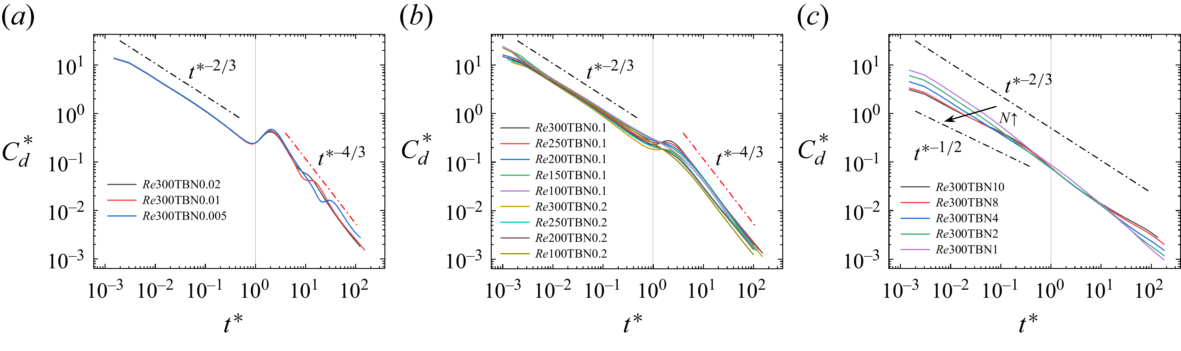
For short time scales
 $t^* \ll 1$
, as presented in figure 14, the drag coefficient decays according to the scaling law
 ${t^*}^{-2/3}$
for small interaction parameters, while a slower decay is observed for large interaction parameters. The decay scaling law of the drag coefficient without a magnetic field at short time scales has been reported as
 ${t^*}^{-1/2}$
by Basset (Reference Basset1888) in the case of an impulsively started sphere without a magnetic field, whereas our previous work found
 ${t^*}^{-2/3}$
in the impulsively stopped case (Cai et al. Reference Cai, Pan and Ni2022). The discrepancy originates from the formation of a primary vortex ring following the impulsive stop, which induces an outward tendency in the upstream region near the sphere, thereby reducing the surface shear stress and ultimately leading to a faster attenuation of the drag coefficient. In the presence of a streamwise magnetic field, the attenuation rate of the drag coefficient remains comparable to the non-magnetic cases at smaller
 $N$
, but significantly decreases at larger
 $N$
(Cai et al. Reference Cai, Pan and Ni2022). Similarly, under a transverse magnetic field, the decay also follows
 ${t^*}^{-2/3}$
at smaller
 $N$
but slows down at larger
 $N$
, as shown in figure 14. The fact that the decay scaling laws remain identical under both streamwise and transverse magnetic fields can be explained qualitatively by the flow structure. Although the direction of the magnetic field is different, the vortex before the stop is still present and the damping effect of the magnetic field is significantly weak at smaller
 $N$
, indicating that the vortex structure is similar to the case without a magnetic field. The formation and diffusion of the vortex can be demonstrated by the instantaneous streamlines on the symmetry plane, as shown in figure 15. The primary vortex persists both at
 $t^*=0$
and
 $t^*=1$
, and the new vorticity is generated around the sphere at
 $0 \lt t^* \lt 1$
, as shown in figure 15(d) by streamlines of the velocity difference. Therefore, the temporal behaviour of the drag coefficient is the same as in the case without a magnetic field, involving two components: the Stokes effect and the inertia effect. These two effects together determine the decay scaling law
 ${t^*}^{-1/2}{t^*}^{-1/6} \sim {t^*}^{-2/3}$
for
 $t^* \ll 1$
. As a result, at shorter time scales with small
 $N$
, the decay rate of the normalised drag coefficient remains
 ${t^*}^{-2/3}$
, which is nearly identical regardless of the presence and the direction of the magnetic field.
The time history of
 $C_d^*$
at
 ${\textit{Re}}_{\!D} \leqslant 300$
with a transverse magnetic field of different intensity. Results are shown for (a)
 ${\textit{Re}}_{\!D} = 300$
with smaller
 $N$
, (b) small
 $N$
with different
 ${\textit{Re}}_{\!D}$
, (c)
 ${\textit{Re}}_{\!D}=300$
with larger
 $N$
.

Instantaneous streamlines on the X–Z plane at
 ${\textit{Re}}_{\!D}=270$
with
 $N=0.1$
. The blank part represents the impulsively stopped sphere. Results are shown for (a)
 $t^*=0$
, (b)
 $t^*=1$
, (c)
 $t^*=15$
. (d) Difference between
 $t^*=0$
and
 $t^*=1$
. (e) Difference between
 $t^*=14$
and
 $t^*=15$
.

Instantaneous streamlines on two symmetry planes at
 ${\textit{Re}}_{\!D}=300$
with
 $N=1$
at different time scales. The blank part represents the impulsively stopped sphere. Results are shown for (a) the X–Z plane at
 $t^*=1$
, (b) the Y–Z plane at
 $t^*=1$
, (c) the X–Z plane at
 $t^*=10$
, (d) the Y–Z plane at
 $t^*=10$
.

With the increment of the interaction parameter, the damping effect of the magnetic field is strong enough to suppress thoroughly the vortex shedding before the stop. Meanwhile, the double-plane symmetry of the flow structure is enhanced by the stronger transverse magnetic field. On the X–Z symmetry plane, vortices remain visible on the upstream side, as shown in figure 16(a). The formation mechanism is similar to that described in figure 3. Unlike in low-
 $N$
cases, however, the upstream vortices remain nearly stationary, without inducing significant inertial convection effects due to their lack of motion. Nonetheless, the MHD effect due to the dissipation of vortex intensity still exists. As a result, the flow pattern on the X–Z plane reflects the combined influence of the origin Stokes part and the MHD part in figure 13, yielding a drag decay scaling law
 $C_d^* \sim {t^*}^{-1/2}{t^*}^{-1/6} \sim {t^*}^{-2/3}$
. On the Y–Z symmetry plane, no vortices are observed in figure 16(b), owing to the stronger damping effect as illustrated in figure 7. Consequently, both the convective and MHD contributions are absent, and the drag decays at a slower rate and tends to a
 ${t^*}^{-1/2}$
scaling with the Stokes effect as the sole governing mechanism. As the interaction parameter increases, the flow pattern on the Y–Z plane, characterised by the Stokes-like behaviour, gradually dominates the overall dynamics, leading the drag decay scaling law to transition from
 ${t^*}^{-2/3}$
to
 ${t^*}^{-1/2}$
, as shown in figure 14(c).
For long time scales
 $t^* \gg 1$
, as shown in figure 14(a,b), the scaling law
 $C_d^* \sim {t^*}^{-4/3}$
under a transverse magnetic field is observed for small interaction parameters. For weak magnetic field intensities and
 ${\textit{Re}}_{\!D}=300$
, vortex shedding still occurs from the sphere for
 $t^*\lt 0$
, although the shedding period increases with the magnetic field intensity, as reported by Pan et al. (Reference Pan, Zhang and Ni2019b
). The detached vortex at
 $t^*\lt 0$
moves downstream at
 $t^*\gt 0$
due to inertia, interacting with the sphere and leading to oscillations in
 $C_d^*$
, as shown in figure 14(a). The oscillations of
 $C_d^*$
at
 $t^* \approx 1$
and
 $t^* \gg 1$
arise from the same underlying mechanism: the contrary influence of the vortex depending on its position relative to the sphere. When the vortex resides on the upstream side, it pulls streamlines away from the sphere surface, reducing the local shear stress. As the vortex propagates downstream, it pushes streamlines closer to the sphere surface, enhancing the shear stress. In addition, the low-pressure region associated with the vortex also travels from the upstream to the downstream side, further contributing to the oscillations in
 $C_d^*$
. However, despite the presence of oscillations, the scaling law
 $C_d^* \sim {t^*}^{-4/3}$
remains clearly evident. When the magnetic field is slightly stronger or when
 ${\textit{Re}}_{\!D}\lt 270$
, no vortex shedding occurs from the sphere at
 $t^*\lt 0$
. As a result, the oscillations in
 $C_d^*$
at long time scales disappear, as shown in figure 14(b). The propagation and evolution of the vortex at long time scales is illustrated in figure 15(c,e). The primary vortex appearing at short time scales propagates downstream and gradually dissipates. However, the residual wake gives rise to new vortices on the upstream side of the sphere, which dominates the variation of the drag coefficient. Meanwhile, the damping effect of the transverse magnetic field causes the vorticity magnitude to decay over time. Therefore, all three components in figure 13 need to be considered, i.e. the origin Stokes effect
 ${t^*}^{-1}$
at long time scales reported by Lawrence & Mei (Reference Lawrence and Mei1995), the inertia effect and the MHD effect. Consequently, the scaling law at
 $t^* \gg 1$
can be derived as
 $C_d^* \sim {t^*}^{-1}{t^*}^{-1/6}{t^*}^{-1/6} \sim {t^*}^{-4/3}$
.
Difference of streamlines at long time scales, at
 ${\textit{Re}}_{\!D}=200$
, with and without a transverse magnetic field. (a) Without a magnetic field; (b) with a transverse magnetic field,
 $N=0.1$
; (c) contour of the X component of the Lorentz force at
 $t^*=1$
.

In the absence of a magnetic field, the drag decay scaling law at long time scales within the range
 $60 \leqslant {\textit{Re}}_{\!D} \leqslant 250$
is previously found to follow a temporal decay of
 ${t^*}^{-1}$
(Cai et al. Reference Cai, Pan and Ni2022). In contrast, when a transverse magnetic field is applied here, both the inertia and MHD effects are incorporated as corrections to the original Stokes contribution in the drag decomposition model at long time scales. The MHD effect arises naturally from the imposition of the magnetic field. However, the inertia effect, which is negligible in non-magnetic cases, becomes significant under the influence of the transverse magnetic field. This difference is primarily attributed to the presence of vortex structures on the local upstream side of the sphere, which persist due to the Lorentz force and consequently influence the incoming flow after the impulsive stop. The instantaneous streamlines on the symmetry plane at long time scales, at
 ${\textit{Re}}_{\!D}=200$
, with and without a transverse magnetic filed, are shown in figure 17(a,b). After the sphere is impulsively stopped, the residual wake is convected downstream and away from the centreline due to the presence of the sphere. As a result, no vortex structures appear in the local inflow zone marked by the red rectangle in the absence of a magnetic field. However, the Lorentz force under a transverse magnetic field confines the wake closer to the centreline at short time scales, as shown in figure 17(c), allowing the upstream vortices in the local inflow zone to influence the flow impacting on the sphere at long time scales. Consequently, the inertia effect associated with the convection effect of vortices must be accounted for when applying a transverse magnetic field with small
 $N$
. At long time scales, both the inertia and MHD effects are coupled with the original Stokes effect, leading to the drag decay scaling
 $C_d^* \sim {t^*}^{-1}{t^*}^{-1/6}{t^*}^{-1/6} \sim {t^*}^{-4/3}$
, which is consistent with simulation results as shown in figure 14(b).
Under a stronger magnetic field, the vortex near the X–Z plane lacks sufficient energy to propagate to the downstream side. In contrast to cases with smaller interaction parameters, the primary vortex appears to be effectively trapped on the upstream side due to the pronounced damping induced by the Lorentz force. As a consequence, the vortex remains upstream even at long time scales, as illustrated in figure 16(c), leading to the absence of oscillations in the time evolution of the normalised drag coefficient
 $C_d^*$
. Moreover, the temporal decay of
 $C_d^*$
at
 $t^* \gg 1$
follows the same decay scaling law,
 $C_d^* \sim {t^*}^{-2/3}$
, as that observed at
 $t^* \ll 1$
in figure 14(c). This behaviour can be qualitatively understood from the perspective of flow structure evolution. The damping effect of the transverse magnetic field is strong enough to suppress the formation of a complete vortex ring at short time scales. Meanwhile, at long time scales, no vortex in the wake moves downstream. Therefore, the flow structure remains similar at both short and long time scales. As a result, the scaling law governing the decay of
 $C_d^*$
remains consistent across different time scales.
4.3. Extension to higher
${\textit{Re}}$

The time history of
 $C_d^*$
at
 ${\textit{Re}}_{\!D}=500$
and
 $1000$
without a magnetic field. The average value of
 $C_d^*$
is averaged for different stopped times. Results are shown for (a)
 ${\textit{Re}}_{\!D}=500$
and (b)
 ${\textit{Re}}_{\!D}=1000$
.

At higher Reynolds numbers, increasingly complex vortex structures emerge in the wake of the sphere, and the applicability of the formerly constructed drag decomposition model is examined. At
 ${\textit{Re}}_{\!D}=500$
and
 $1000$
, the large-scale wake structures remain clearly observable and the drag coefficient continues to follow a power-law decay. Considering the combined contributions of the Stokes effect and inertia effects, as illustrated in figure 13, the temporal evolution of the normalised drag coefficient follows
 $C_d^* \sim {t^*}^{-1/2}{t^*}^{-1/6} \sim {t^*}^{-2/3}$
at short time scales and
 $C_d^* \sim {t^*}^{-1}{t^*}^{-1/6} \sim {t^*}^{-7/6}$
at long time scales. These scaling predictions show better agreement with the simulation results than the original ones, as shown in figure 18. As mentioned in § 3, in the absence of a magnetic field, the flow field exhibits unsteady vortex shedding at
 ${\textit{Re}}_{\!D}=1000$
during the fully developed stage prior to the impulsive stop of the sphere. Therefore, to analyse the general evolution, drag coefficients from cases with varying stop times are averaged. Eight stop times are selected, uniformly distributed within a single primary vortex-shedding period. Similar to the cases with lower Reynolds numbers and interaction parameters, the decay scaling behaviour
 ${t^*}^{-2/3}$
remains essentially unchanged, as presented in figure 18. Notably, a significant fluctuation in
 $C_d^*$
occurs near
 $t^*=1$
, including a reversal in its direction. This behaviour results from the exclusion of negative values on the log–log scale. After the impulsive stop of the sphere, the upstream fluid continues moving forward and interacts with the sphere. Due to the acceleration effect caused by the sphere’s curved surface, the flow velocity near the upstream-facing side of the sphere increases, forming a low-pressure region. The low-pressure region continues to move downstream and gradually dissipates due to viscous and magnetic damping effects, as shown in figure 19. As a result, a significant fluctuation occurs in the pressure drag, which in turn causes a fluctuation in the total drag. At long time scales, the complex wake structures cause the drag decay to exhibit rather chaotic behaviours. However, the averaged overall trend still remains more consistent with the scaling laws derived from the drag decomposition framework than with the original ones.
Pressure contours of
 $t^*=1$
and
 $t^*=2$
at
 ${\textit{Re}}_{\!D}=1000$
without a magnetic field. The stopped instant
 $t_{\textit{stop}}=0.75T$
.

The time history of
 $C_d^*$
at
 ${\textit{Re}}_{\!D}=1000$
with different interaction parameters. (a) Relatively large
 $N$
; (b) relatively larger
 $N$
.

Instantaneous streamlines on the symmetry plane X–Z at
 ${\textit{Re}}_{\!D}=1000$
with
 $N=0.3$
. The blank part represents the impulsively stopped sphere. Results are shown for (a)
 $t^*=1$
and (b)
 $t^*=15$
.

Instantaneous streamlines on two symmetry planes at
 $t^*=15$
at
 ${\textit{Re}}_{\!D}=1000$
with
 $N=10$
. The blank part represents the impulsively stopped sphere. Results are shown for the (a) X–Z plane and (b) the Y–Z plane.

When a transverse magnetic field is applied, the temporal decay of the drag coefficient follows a
 ${t^*}^{-5/6}$
scaling for large
 $N$
and a
 ${t^*}^{-2/3}$
scaling for larger
 $N$
, as shown in figure 20. As shown in figure 10, when the magnetic field is not very strong, vortex shedding still occurs from the sphere surface before the impulsive stop. Under the influence of the transverse magnetic field, the flow around the sphere exhibits double-plane symmetry. The streamlines on the X–Z symmetry plane, as shown in figure 21, reveal the presence of persistent upstream vortex structures that propagate downstream due to inertia. As a result, the inertial convection induced by these vortex structures remains significant. Meanwhile, due to the damping effect of the transverse magnetic field on vortices, the MHD effect must also be accounted for. Consequently, the drag is corrected by both the inertia effect and MHD effect based on the Stokes effect. Therefore, the scaling law becomes
 $C_d^* \sim {t^*}^{-1/2}{t^*}^{-1/6}{t^*}^{-1/6} \sim {t^*}^{-5/6}$
by incorporating the three effects. At long time scales, the main vortex structures concentrate on the upstream side and remain similar to that at short time scales as shown in figure 21. As a result, the decay rate of
 $C_d^*$
at long time scales is consistent with that observed at short time scales. However, when the magnetic field is sufficiently strong to suppress the downstream propagation of vortices, the vortex structures appear frozen on the upstream side, as illustrated by the instantaneous streamlines at long time scales in figure 22(a). Consistent with the case of
 ${\textit{Re}}_{\!D}=300$
, the streamlines indicate that the flow around the Y–Z plane is similar to the Stokes flow as shown in figure 22(b). Thus, the MHD effect
 ${t^*}^{-1/6}$
combines with the Stokes contribution
 ${t^*}^{-1/2}$
, resulting in an overall scaling law of
 ${t^*}^{-2/3}$
, as shown in figure 20(b). Although the vortex structures become increasingly complex at higher Reynolds numbers, the reasonable extension of the drag decomposition model gives the explanation for the drag decay with three effects in figure 13 across various parameters. The derived scaling laws exhibit better consistency with the simulation results than the original scaling laws.
4.4. Extension to prolate spheroid
The alteration of particle shape can lead to increasing flow complexity. Specifically, the geometric anisotropy of a prolate spheroid introduces additional asymmetry into the flow field after an impulsive stop. In this context, the applicability of the established drag decomposition model is further examined. In the moderate Reynolds number regime, the drag coefficient formula of a prolate spheroid is given by the correlation proposed in Fröhlich et al. (Reference Fröhlich, Meinke and Schröder2020):
 \begin{align} C_d^{\theta } = \frac {24}{{{\textit{Re}}}_{d_e}} g_{\theta }(\beta )\left (1+0.15 {{{\textit{Re}}}_{d_e}^{0.687}} + c_{\theta ,1}(\log \beta )^{c_{\theta ,2}} {{{\textit{Re}}}_{d_e}}^{c_{\theta ,3} + c_{\theta ,4} \log \beta }\right )\! .\end{align}
Here
 $\theta$
is the inclination angle between the free-stream velocity and the spheroid’s long axis,
 $\beta$
is the aspect ratio between the long axis and the short axis, and
 $g_{\theta }(\beta )$
is a function relevant to the geometric shape parameters. The coefficients
 $c_{\theta ,i}$
are empirical fitting parameters. In the general definition of
 ${{\textit{Re}}}_{d_e}$
, the volume-equivalent diameter
 $d_e$
is adopted as the characteristic length. It is noted that
 $c_{\theta , 1}$
is generally at least one order of magnitude smaller than the preceding term coefficient
 $0.15$
. Moreover,
 $g_{\theta }$
depends solely on the shape parameters and is independent of the Reynolds number. Consequently, the drag decay scaling law remains the same behaviour as that for a sphere, regardless of the aspect ratio
 $\beta$
or the inclination angle
 $\theta$
.
The time history of
 $C_d^*$
for a prolate spheroid with different configuration parameters. The legend in the plot, for example, `AR4an90Re200T1’ indicates that
 $\beta =4$
,
 $\theta =90^\circ$
,
 ${{\textit{Re}}}_{d_e}$
= 200 and
 $t_{\textit{stop}}=1/4T$
, where
 $T$
is the vortex-shedding period prior to the impulsive stop. (a) Relatively low
 ${{\textit{Re}}}_{d_e}$
, no oscillations appearing at
 $t^* \gg 1$
; (b) relatively high
 ${{\textit{Re}}}_{d_e}$
, oscillations appearing at
 $t^* \gg 1$
.

Temporal evolution of vortex structures around a prolate spheroid (
 $\beta =4$
,
 $\theta =90^\circ$
) at
 ${{\textit{Re}}}_{d_e}=100$
and
 ${{\textit{Re}}}_{d_e}=200$
. Results are shown for (a)
 ${{\textit{Re}}}_{d_e}=100$
, visualised using the instantaneous streamlines on the symmetry plane (Y–Z plane); (b)
 ${{\textit{Re}}}_{d_e}=200$
, visualised using the Q-criterion (
 $Q_{\textit{criterion}}=0.1$
).

The time history of
 $C_d^*$
after the impulsive stop for a prolate spheroid with different
 $\beta$
,
 $\theta$
and
 ${{\textit{Re}}}_{d_e}$
is presented in figure 23. For short time scales
 $t^* \ll 1$
, all configurations exhibit a drag decay following the scaling law
 $C_d^* \sim {t^*}^{-2/3}$
. For long time scales
 $t^* \gg 1$
, the drag decays as
 ${t^*}^{-1}$
at relatively low
 ${{\textit{Re}}}_{d_e}$
and as
 ${t^*}^{-7/6}$
at relatively high
 ${{\textit{Re}}}_{d_e}$
where unsteady vortex shedding is present prior to the impulsive stop. As
 $\beta$
approaches unity, the spheroid geometry approaches that of a sphere, while larger
 $\beta$
introduces greater anisotropy. Therefore, cases with
 $\beta = 4$
are selected to visualise the vortex structures and examine the validity of the drag decomposition model. The temporal evolution of the vortex structures around an impulsively stopped prolate spheroid with
 $\beta =4$
and
 $\theta =90^\circ$
is presented in figure 24. At
 ${{\textit{Re}}}_{d_e}=200$
, the wake exhibits periodic vortex shedding in the fully developed stage prior to the impulsive stop. To capture this vortex-shedding behaviour, the vortex evolution is visualised using the Q-criterion. However, at
 ${{\textit{Re}}}_{d_e}=100$
, the wake remains steady and exhibits double-plane symmetry prior to the impulsive stop, so the evolution process is visualised by streamlines on the symmetry plane. The X-Z plane is chosen for comparison, as the vortex shedding at
 ${{\textit{Re}}}_{d_e}=200$
primarily develops around this plane. At short time scales, the primary vortex forms upstream near the spheroid for both
 ${{\textit{Re}}}_{d_e}=100$
and
 $200$
. Therefore, the inertia effect must be incorporated with the Stokes effect in the drag decomposition model, leading to
 ${C_d}^* \sim {t^*}^{-1/2}{t^*}^{-1/6} \sim {t^*}^{-2/3}$
, which is consistent with the simulation results shown in figure 23 at
 $t^* \ll 1$
.
At long time scales, the drag decay at moderate
 ${{\textit{Re}}}_{d_e}$
is surprisingly found to still follow the same scaling law as that derived by Lawrence & Mei (Reference Lawrence and Mei1995) for a sphere at the low-Reynolds-numbers regime, following the temporal decay of
 ${t^*}^{-1}$
. The flow around a prolate spheroid involves both the long-axis and short-axis sides. Due to its geometry, thicker in the middle and tapered at both ends, the majority of the drag arises from the abdominal region. Therefore, the vortex structures developing near the short-axis side have a more pronounced influence on the overall drag evolution. After the impulsive stop, the primary vortex propagates downstream and radially outward from the centreline, driven by its self-induced radial velocity. Due to the smaller cross-section on the short-axis side and the steady flow prior to the impulsive stop, no upstream vortex structure forms in the local region near the upstream side of the spheroid at long time scales, as shown in figure 24(a). As a result, the upstream flow impacting on the spheroid at long time scales resembles that in the low-Reynolds-number regime for a sphere. This suggests that the Stokes effect can still be defined as
 ${t^*}^{-1}$
at long time scales in the drag decomposition model. At
 ${{\textit{Re}}}_{d_e}=200$
, a sequence of accompanying vortices move downstream as shown in figure 24(b), influencing the inflow impacting on the spheroid. As a result, the inertia effect must again be combined with the Stokes effect, giving
 ${C_d}^* \sim {t^*}^{-1}{t^*}^{-1/6} \sim {t^*}^{-7/6}$
, which aligns well with the simulation results presented in figure 23(b) for
 $t^* \gg 1$
. To further examine the inertia effect
 ${t^*}^{-1/6}$
in the drag decomposition model at moderate
 $\theta$
, the time history of
 $C_d^*$
and evolution of vortex structures for a prolate spheroid with
 $\beta =4$
and
 $\theta =75^\circ$
are presented in figure 25. Under this configuration, the wake prior to the impulsive stop exhibits periodic vortex shedding. After the impulsive stop, a primary vortex forms upstream at short time scales and a sequence of accompanying vortices on the upstream side impacts on the spheroid at long time scales. Therefore, the drag decay must incorporate the inertia effect with the Stokes effect both at short and long time scales, leading to the decay law
 ${C_d}^* \sim {t^*}^{-1/2}{t^*}^{-1/6} \sim {t^*}^{-2/3}$
for
 $t^*\ll 1$
and
 ${C_d}^* \sim {t^*}^{-1}{t^*}^{-1/6} \sim {t^*}^{-7/6}$
for
 $t^*\gg 1$
. Although the spheroid is notably prolate with
 $\beta =1.5, 2.5, 4$
and inclined with
 $\theta =0^\circ , 75^\circ , 90^\circ$
, the drag decomposition model presented in figure 13 successfully predicts the drag decay scaling law by reasonably extending the framework to incorporate the evolution of the vortex structures. At
 $t^* \sim 1$
, the vortex structures around the spheroid are significantly influenced by its shape, but the coefficient of the shape-correction term is relatively small compared with the inertial contribution and was therefore neglected. Nevertheless, the proposed scaling laws still capture the overall decay trend more accurately than the uncorrected laws.
The time history of
 $C_d^*$
and temporal evolution of vortex structures for a prolate spheroid with
 $\beta =4$
and
 $\theta =75^\circ$
at
 ${{\textit{Re}}}_{d_e}=250$
. (a) Time history of
 $C_d^*$
; (a) vortex structures at different
 $t^*$
, visualised using the Q-criterion (
 $Q_{\textit{criterion}}=0.1$
).

4.5. Extension to magnetic fields with different directions
In realistic situations the magnetic field is not necessarily aligned or perpendicular to the primary flow direction. Therefore, it is essential to extend the analysis to magnetic fields with different orientations. Before introducing an inclined magnetic field, the streamwise configuration is re-examined here after our previous work (Cai et al. 2022). The slight difference between the streamwise and transverse cases about the drag decay exists in the small and medium interaction numbers regime. However, for strong magnetic fields, a new drag decay law at long time scales is identified.
The time history of
 $C_d^*$
after the impulsive stop for different interaction parameters is shown in figure 26. When
 $N$
is relatively small, the streamwise magnetic field is too weak to noticeably influence the vortex structure and vorticity transport. Accordingly, the drag decay follows the same scaling laws as those without a magnetic field, only including the Stokes effect and the inertia effect. This leads to the decay scaling law
 ${C_d}^* \sim {t^*}^{-1/2} {t^*}^{-1/6} \sim {t^*}^{-2/3}$
at short time scales and
 ${C_d}^* \sim {t^*}^{-1} {t^*}^{-1/6} \sim {t^*}^{-7/6}$
at long time scales. The difference between the streamwise and transverse cases arises primarily from the angle between the magnetic field and the main flow direction. In the transverse configuration the nearly perpendicular alignment causes the MHD effect to appear even at small interaction parameters, whereas the nearly parallel configuration delays the effect under the same parameters. When
 $N$
reaches moderate values, the drag decay scaling law is consistent with that at smaller Reynolds numbers without a magnetic field, as presented in figure 26(b). In this regime, the inertia effect must be considered at short time scales but it becomes negligible at long time scales. While no vortex structures were observed in the key region at long time scales in figure 17 (§ 4.2), a primary vortex does exist in the upstream zone at short time scales, as shown in figure 27. As a result, both the Stokes effect and inertia effect are included at short time scales, whereas only the Stokes effect remains at long time scales, leading to
 ${C_d}^* \sim {t^*}^{-1/2} {t^*}^{-1/6} \sim {t^*}^{-2/3}$
at short time scales and
 ${C_d}^* \sim {t^*}^{-1}$
at long time scales.
The time history of
 $C_d^*$
at
 ${\textit{Re}}_{\!D} = 300$
with a streamwise magnetic field of different intensity. (a) Smaller
 $N$
; (b) medium
 $N$
; (c) larger
 $N$
.

Instantaneous streamlines on the symmetry plane X–Z at
 ${\textit{Re}}_{\!D}=300$
with
 $N=1$
. The blank part represents the impulsively stopped sphere. Results are shown for (a)
 $t^*\approx 1$
and (b)
 $t^*=10$
.

Instantaneous streamlines on the symmetry plane X–Z at
 ${\textit{Re}}_{\!D}=300$
with
 $N=9$
when
 $t^*=10$
, representing longer time scales. The blank part represents the impulsively stopped sphere. (a) Streamwise magnetic field; (b) transverse magnetic field.

When
 $N$
is large, the drag decays as a different law, exhibiting an exponential decay law at long time scales, as shown in figure 26(c). In applications of the drag formulations, the drag force is often expressed dimensionally as
 $F_d=3\pi \rho \nu U D g({\textit{Re}})$
, where
 $U$
is the real local velocity of the fluid around the sphere and
 $g({\textit{Re}})$
is the drag coefficient as a function of the real local Reynolds number,
 ${\textit{Re}}=UL / \nu$
. The local velocity can be set as
 $U=\gamma (t) U_0$
and then
 ${\textit{Re}}=\gamma (t) {\textit{Re}}_0$
. When
 $\gamma (t) \ll 1$
, the drag can be expanded at zero as
 \begin{equation} F_d \sim \gamma (t) g(\gamma {\textit{Re}}_0) \sim \gamma (t)g(0) + \gamma ^2(t) g'(0) {\textit{Re}}_0 + {\cdots} \sim \gamma (t), \quad \gamma (t) \ll 1. \end{equation}
Consequently, the drag decay follows the same functional form as the velocity decay, both exhibiting either a power-law decay or an exponential behaviour. When the magnetic field is aligned with the flow direction, the streamlines are confined with a narrow region in the wake. In the wake region the electric current arising from electromotive effects plays a more significant role than electrostatic potential effects. The electric current density is dominated by the partial Ohm’s law,
 $\boldsymbol{{J}} \approx \boldsymbol{{u}} \times \boldsymbol{{B}}_0$
. At sufficiently large values of
 $N$
, the contribution of the Lorentz force becomes more important than other terms in the momentum equation. Accordingly, the relation between the fluid velocity and the Lorentz force can be approximated as
 $ {\partial \boldsymbol{{u}}}/{\partial t} \sim N (\boldsymbol{{J}} \times \boldsymbol{{B}}_0 ).$
Substituting the partial Ohm’s law and following a straightforward derivation, the simplified velocity decay can be expressed as
 \begin{equation} {|\boldsymbol{{u}}|} \sim U_0 e^{-f\left (N\right )t} \sim \gamma (t) U_0. \end{equation}
At long time scales, the velocity magnitude becomes small and
 $\gamma (t) \ll 1$
is satisfied. Hence, the drag decay follows the same exponential form as the velocity, as presented in figure 26. The difference between the streamwise and transverse cases arises primarily from the different vortex structures as presented in figure 28. In MHD flows, a strong magnetic field prompts vortices to tend to be parallel to its direction, so the upstream vortex observed in the transverse case does not form for a streamwise magnetic field. Moreover, the strong streamwise magnetic field confines the vorticity to a narrow region around the sphere. The mechanism of vorticity transport dominating the drag decay gradually loses the leading role. As a result, the drag decay law in the streamwise case is dominated by the velocity decay rather than by the vortex-induced effects.
The time history of
 $C_d^*$
at
 $\textit{Re}_D=300$
and
 $N=0.1$
for a magnetic field with different directions.

After examining the two extreme configurations for the direction of a magnetic field, cases with a magnetic field of any direction were then also investigated. The angle between the applied magnetic field and the transverse direction is set to
 $0^\circ$
,
 $30^\circ$
,
 $45^\circ$
,
 $60^\circ$
and
 $90^\circ$
, as presented in figure 29. For
 $N=0.1$
, the drag decay exhibits different behaviours between the streamwise and transverse configurations. Therefore, the drag decay at
 ${\textit{Re}}=300$
and
 $N=0.1$
is examined for different magnetic field orientations. As shown in figure 29, the drag decay as
 ${t^*}^{-2/3}$
at short time scales, which is the same as the two extreme configurations. At long time scales, as the magnetic field orientation changes from transverse to streamwise, the drag decay law transitions from
 ${t^*}^{-4/3}$
to
 ${t^*}^{-1}$
. As expected, the changing tendency of the drag decay law is the same as the orientation angle of the magnetic field. The closer the orientation is to either extreme configuration, the more closely its drag decay follows the corresponding scaling law. Although the magnetic field might take any orientation in realistic situations, the drag decay behaviour remains bounded by the two limiting cases.
5. Summary
The flow dynamics around an impulsively stopped sphere immersed in an incompressible, viscous and electrically conducting fluid under a uniform transverse magnetic field has been investigated numerically in detail. The transverse magnetic field is applied from the beginning of all simulations, and the sphere wake has reached a fully developed state after a forced and long enough distance motion with a constant velocity. The study focuses on parameters ranges of
 $60 \leqslant {\textit{Re}}_{\!D} \leqslant 300$
and
 ${\textit{Re}}_{\!D}=1000$
with
 $0\leqslant N \leqslant 10$
. A rich vortex structure system emerges, influenced by the initial state at different Reynolds numbers and interaction parameters. A simplified regime map of wake flow patterns is constructed in the
 $\{N$
,
 ${\textit{Re}}_{\!D}\}$
phase space based on nearly 200 simulation cases. The categorisation is based on topological features of the skin friction lines on the downstream sphere surface, including the presence of convergent/divergent nodes and a closed or straight convergent line. Due to the presence of a transverse magnetic field, the wake at
 $t^*\gt 0$
inherently retains planar symmetry, with the symmetry plane oriented perpendicular to the magnetic field direction. As a result, all observed skin friction patterns also possess planar symmetry. At higher Reynolds number (
 ${\textit{Re}}_{\!D} = 1000$
), the enhanced anisotropy damping effect of the magnetic field leads to the emergence of a gourd-shaped convergent line in the skin friction lines topology, a feature that can also be incorporated into the regime categorisation established at
 $60 \leqslant {\textit{Re}}_{\!D} \leqslant 300$
. Moreover, the so-called `reversion phenomenon’ is reaffirmed, indicating that the flow patterns around a sphere at higher
 ${\textit{Re}}_{\!D}$
and higher
 $N$
correspond to those observed at lower
 ${\textit{Re}}_{\!D}$
and lower
 $N$
.
Furthermore, the decay of drag coefficient after the sphere stops is investigated. Motivated by the classical first Stokes problem, the vorticity diffusion scale is introduced as a dynamic characteristic length for the Reynolds number during the decay process. Utilising this time-dependent length scale, the temporal evolution of the drag coefficient can be simply derived by the drag coefficient formula. A drag decomposition model is constructed to decompose the drag into three principal contributions: the original Stokes drag component and two correction factors arising from inertia and MHD effects. As to which of the three components predominantly contribute to the resulting decay scaling laws is based on the flow structures, which depends on
 ${\textit{Re}}_{\!D}$
,
 $N$
and the characteristic time scale. At shorter time scales, the normalised drag coefficient
 ${C_d}^*$
follows an algebraic decay of
 ${t^*}^{-2/3}$
for relatively small interaction parameters within
 $60 \leqslant {\textit{Re}}_{\!D} \leqslant 300$
. As
 $N$
increases, the decay rate decreases slightly but generally remains consistent with the
 ${t^*}^{-2/3}$
scaling. At longer time scales, the decay rate of the drag coefficient approaches either
 ${t^*}^{-4/3}$
or
 ${t^*}^{-2/3}$
, depending on
 $N$
. The established drag decomposition model has been extended to higher Reynolds numbers with the more complex vortex evolution and a prolate spheroid with an anisotropy geometry. For
 ${\textit{Re}}_{\!D}=1000$
and
 $N=0$
,
 ${C_d}^*$
initially decays algebraically as
 ${t^*}^{-2/3}$
at shorter time scales. However, at longer time scales, the presence of numerous secondary vortices induces chaotic oscillations, while the averaged decay rate asymptotically follows
 ${t^*}^{-7/6}$
. When
 $N\gt 0$
for
 ${\textit{Re}}_{\!D}=1000$
, the large-amplitude oscillations observed near
 $t^* \approx 1$
are progressively damped and eventually vanish. For large
 $N$
, the decay rate of
 ${C_d}^*$
follows
 ${t^*}^{-5/6}$
, while for larger
 $N$
, it converges towards
 ${t^*}^{-2/3}$
. As for the impulsively stopped spheroid, the drag decay scaling law exhibits a similar behaviour with the sphere, i.e.
 ${C_d}^*$
follows a decay law of
 ${t^*}^{-2/3}$
at short time scales and a decay law of
 ${t^*}^{-1}$
or
 ${t^*}^{-7/6}$
at long time scales depending on the presence of accompanying vortices. Although the vortex structures become increasingly complex at higher Reynolds numbers and the prolate spheroid introduces geometric anisotropy, the drag decomposition model proposed here, with appropriate extensions, successfully captures the drag decay following an impulsive stop. This demonstrates its capability to reveal the underlying physical mechanisms governing the drag decay.
Moreover, cases with different magnetic field orientations are examined. In the streamwise configuration the drag decay is identified to be consistent with the results based on the drag decomposition framework in both the small and moderate
 $N$
regimes. For large
 $N$
, an exponential decay law is identified at long time scales. Across various magnetic field orientations, the drag decay behaviour remains bounded by the two extreme configurations. This continuous transition makes the drag decay law more broadly applicable to realistic situations.
Funding
The authors gratefully acknowledge support from National Key Research and Development Program of China (2022YFE03130000), National Natural Science Foundation of China (12472260, U23B20110, 12388101), Innovation Special Project of the Bureau of Major Science and Technology Programs by CAS(RCJJ-145-24-58) and Young Elite Scientists Sponsorship Program by CAST (2022QNRC001).
Declaration of interests
The authors report no conflict of interest.
Appendix A. Flow details
A.1. Flow in the fully developed stage at
${{\textit{Re}}_{\!D}}=300$
with various
$N$


Instantaneous streamlines in the fully developed stage at
 ${\textit{Re}}_{\!D}=300$
with various
 $N$
. The streamlines on the symmetry planes at
 $t^* = 0$
are shown with the common contour legend in the first plot. The first plot displays streamlines on a single symmetry plane, while the remaining plots in the row show results on two symmetry planes for half of the plot. (a) Results are shown for
 $N=0.05$
, (b)
 $N=0.2$
, (c)
 $N=0.5$
, (d)
 $N=4$
.

The wake in the fully developed stage induced by a moving sphere with a transverse magnetic field is significantly different from that without a magnetic field. To better understand the flow field after the sphere stops impulsively, streamlines on the symmetry planes for the fully developed wake structure are shown in figure 30. At
 $ Re_D = 300$
with
 $N=0.05$
, the wake exhibits single plane symmetry so the first plot in the figure 30 displays streamlines on a single symmetry plane.
A.2. Details about wake evolution at
${\textit{Re}}_{\!D} = 1000$

A detailed description about the wake evolution at
 $ Re_D = 1000$
is provided here. Following the impulsive stop (
 $t^* \gt 0$
), the residual kinetic energy remains sufficiently large for the vorticity to detach from the sphere surface. The downstream vorticity rolls up to form a LVS, while the upstream vortex is convected downstream, giving rise to the first vortex structure (VS-1). Subsequently, driven by the induced flow of VS-1 and the remaining wake energy, the second vortex structure (VS-2) forms and gradually detaches from the sphere surface. During this process, numerous hairpin-shaped vortices originating from the previous wake interact with the sphere and with VS-1 and VS-2, as shown in figure 31. Their legs are wrapped by the surrounding large-scale structures, producing transient radial vortices. The complexity inherited by the old wake, combined with the interactions among multiple vortex structures, gives rise to the three-dimensional instability. As a result, the vortex system evolves into an increasingly complicated structure and gradually dissipates through convection and viscous diffusion until it vanishes.
When a transverse magnetic field is applied, the evolution pathway of these vortices is significantly modified, as illustrated in figure 32. The Lorentz force suppresses the Kelvin–Helmholtz instability, effectively damping the formation of small-scale vortices that are otherwise abundant in the non-magnetic case. Therefore, such small-scale structures are scarcely observed during the wake evolution and the flow remains more coherent and symmetric. The detachment of VS-2 is also restrained due to suppression effects. The LVS remains partially connected to VS-1, primarily in the Y–Z plane, due to anisotropic magnetic damping. Meanwhile, the residual hairpin vortices from the old wake propagate downstream and promote the splitting of the secondary vortex pair (VSP-2) along the X axis. Under the curling effect of VS-1, VSP-2 evolves into two closed vortex rings, and a new secondary ring (NVS-2) appears near the sphere as the residual wake continues to impact on the body. Throughout this evolution, the wake preserves its double-plane symmetry and exhibits markedly reduced small-scale activity compared with the non-magnetic case.
Temporal evolution of downstream vortex structures, at
 ${\textit{Re}}_{\!D}=1000$
, without a magnetic field, visualised using the Q-criterion (
 $Q_{\textit{criterion}}=1$
) . Results are shown for (a)
 $t^*=1$
, (b)
 $t^*=2$
, (c)
 $t^*=3$
, (d)
 $t^*=5$
. Here VS-1 and VS-2 indicate the first and second vortex ring structures, respectively.

Temporal evolution of vortex structures downstream visualised using the Q-criterion (
 $Q_{\textit{criterion}}=1$
) at
 ${\textit{Re}}_{\!D}=1000$
with
 $N=0.3$
. Results are shown for (a)
 $t^*=1$
, (b)
 $t^*=3$
, (c)
 $t^*=5$
. Here VS-1 and VSP-2 represent the first vortex structure and the second vortex pair, respectively; NVS-2 denotes the newly formed vortex ring.

Appendix B. Summary of simulation cases
For greater transparency, simulation cases of the present work are summarised in tables 2 and 3, corresponding to simulation cases of the stopped sphere and the prolate spheroid, respectively. The parameter space covers 13
 $ Re_D$
and 26
 $N$
values. Values greater than one listed in the two tables indicate the number of simulation cases performed at the same
 $ Re_D$
and
 $N$
but with different stopped instants.
Summary of simulation cases. The number in the table represents the number of simulation cases with the same
 ${\textit{Re}}_{\!D}$
and
 $N$
but different stopped instants. The parameter space includes 13
 ${\textit{Re}}_{\!D}$
and 26
 $N$
values.

Summary of simulation cases of a prolate spheroid. The parameters
 $\beta$
,
 $\theta$
and
 ${{\textit{Re}}}_{d_e}$
represent the aspect ratio between the long axis and the short axis, the inclination angle between the free-stream velocity and the spheroid’s long axis, and the Reynolds number with the volume-equivalent diameter
 $d_e$
as the characteristic length scale, respectively.