Threshold searchers: the ‘supply side’ approach

This involves plotting the marginal health gain (MHG) of health care expenditures, dH/dE, against health care expenditures, E. Figure 1, taken from Culyer et al. (Reference Culyer, McCabe, Briggs, Claxton, Buxton, Akehurst, Sculpher and Brazier2007), presents the case of the MHG diminishing at a constant rate. Interventions appear in descending order of MHG (or what the authors call the ‘impact on health per pound spent’) (i.e., line ha, Figure 1).

Figure 1

Marginal health gain from current interventions. Based on Culyer et al. (Reference Culyer, McCabe, Briggs, Claxton, Buxton, Akehurst, Sculpher and Brazier2007)

Once resources, E*, have been exhausted no more interventions can be funded. The authors note that MHG at this point, a, represents the inverse of the marginal cost-effectiveness of expenditure (Culyer et al., Reference Culyer, McCabe, Briggs, Claxton, Buxton, Akehurst, Sculpher and Brazier2007: 57),Footnote ¹ which they interpret to be the “threshold incremental cost-effectiveness ratio”. This implicitly assumes that MHG is equal to the incremental health gain (IHG) and the MC is equal to the incremental cost, (or alternatively, the ratio of MHG to MC is equal to the ICER). Only under these assumptions, could we expect to have the downward sloping straight line for MHG.

Figure 2 (from Culyer et al., Reference Culyer, McCabe, Briggs, Claxton, Buxton, Akehurst, Sculpher and Brazier2007) introduces the MHG for interventions not currently funded, cf, and the solution to allocating expenditure E* between all possible interventions by aggregating expenditures horizontally to give hde. Optimal allocation is determined by adopting interventions in descending order of MHG up to E*. This requires 0E' be allocated to existing interventions and E'E* (=E*E'') to new interventions. Funds have been reallocated from interventions with lower MHG to interventions with higher MHG. The marginal cost-effectiveness of expenditure has increased to E*b (>E*a), the area under the new MHG curve (hdb) is greater than in Figure 1 and total health gains from E* (and efficiency of resource use) has increased.

Figure 2

Allocating expenditures with new interventions. Based on Culyer et al. (Reference Culyer, McCabe, Briggs, Claxton, Buxton, Akehurst, Sculpher and Brazier2007)

However, MHG is given by comparing the health gain from an intervention with the health gain that would be produced from one less unit of expenditure on the same intervention (i.e., moving along the MHG line) while the IHG is the difference between the health gain from the intervention and the health gain from whatever would be done for the same patient population in the absence of the intervention. The assumption of equality between the MHG from additional expenditure and IHG from adoption of a new programme requires that the incremental cost of the new programme equals one indivisible unit of expenditure (i.e., the margin), a very special case with little practical relevance when comparing different health care interventions.

The ICER involves measuring the difference between health gains of the new intervention and the current way of treating the same patient group (IHG), the difference between the costs of the new intervention and the current way of treating the same patient group (incremental costs), and taking the ratio of incremental costs to incremental effects, no matter how large these increments are. The ratio therefore measures the average cost per additional QALY (ACAQ), with its inverse being the average rate of return on (additional) investment (ARRI). When considering new interventions, decision makers are concerned with increments based on the population to receive the intervention as opposed to, for example, the subjects included in a trial, because incremental costs and effects, and hence the opportunity costs, would be substantially different between policy and study populations even if the ICERs were the same.

The use of the ICER or ACAQ for determining the marginal condition for efficiency requires that intra-incremental changes in programmes are possible (perfect divisibility) so that reallocations can be made at the margin. Moreover, it requires that the ACAQ is constant (constant returns to scale) so that the rate of return observed on average for the size of the incremental intervention is the same for intra-incremental changes in intervention size. However, the authors recognise that there is no reason to believe that MHG (and hence the ACAQ) is constant as “people with the best chances of being helped have already been helped” (Culyer et al., Reference Culyer, McCabe, Briggs, Claxton, Buxton, Akehurst, Sculpher and Brazier2007: 57).

Threshold searching is essentially a form of programme budget marginal analysis (PBMA) (Mooney, Reference Mooney2003; Mitton and Donaldson, Reference Mitton and Donaldson2004). A key element of marginal analysis is the comparison of choices directly based on benefits produced (effects of spending one dollar more on intervention A and intervention B). However, health care managers face decisions about investing large amounts of resources on interventions with a mixture of fixed and variable costs. So the usual marginal conditions for efficiency are not relevant. Interventions involve lumpy investments that require different amounts of additional resources and hence cannot be compared directly or reduced to comparable size with other interventions. The threshold searchers and PBMA both use ICERs as indicators of changes in health gains and costs at the margin to compare a new intervention with an intervention it might replace even though the interventions involve different levels of resource investment. This suggests that PBMA might be more appropriately renamed programme budgeting incremental analysis.

Donaldson et al. (Reference Donaldson, Bate, Mitton, Dionne and Ruta2010) mention the problem of ‘lumpy’ investments in terms of rational disinvestment under which expenditure is reduced on interventions generating less health effects than produced by allocating the same expenditure to the new intervention. The authors describe this as marginal analysis, possibly because the changes considered relate to the size of existing interventions, not replacing one intervention with another. However, the ‘lumpiness’ in the changes in interventions gives rise to the problems with marginal analysis (and the need to base analysis on increments), not the nature of the programme comparisons.

Threshold surveyors: the ‘demand side’ approach

This seeks to complement threshold searching with information on societal willingness to pay (WTP) for health gains estimated from individuals’ WTP (Baker et al., Reference Baker, Chilton, Donaldson, Jones-Lee, Lancsar, Mason, Metcalf, Pennington and Wildman2011). Although their conceptual framework differs from the threshold searchers’ framework, it also uses incremental values to measure marginal changes. As a result, it compounds the errors of the threshold searchers’ approach as opposed to enhancing it.

The framework (Figure 3, based on Baker et al. (Reference Baker, Chilton, Donaldson, Jones-Lee, Lancsar, Mason, Metcalf, Pennington and Wildman2011)) involves plotting total benefits, B, and total costs, C, against ‘quantity of health care’, Q. It is not clear how Q is measured, but it is different from expenditure (or costs) because this is on the vertical axis. Benefits are a fixed multiple of Q, B=VQ where V is the fixed ‘value per unit of health care’, which they suggest is the value per QALY. However, this confuses inputs to health production (quantity of health care) with outcomes (QALYs). In other words, fixing V implies a constant marginal productivity of ‘health care’, dQALY/dQ, and a constant marginal valuation of QALYs, dV/dQALY (or the special case where non-constancy in one is offset exactly by non-constancy in the other).Footnote ²

Figure 3

Finding a value of a QALY. Based on Baker et al. (Reference Baker, Chilton, Donaldson, Jones-Lee, Lancsar, Mason, Metcalf, Pennington and Wildman2011)

The authors assume that the MC of health care, dC/dQ, which equals the MC of QALY production under the implicit assumptions, increases even under the modest variations in Q they invoke to justify the constant marginal benefits assumption. The marginal condition for efficiency occurs at Q* where the (constant) marginal benefit (the gradient of the benefit line) equals the (non-constant) MC (the gradient of the total cost curve).

As the opportunity cost of health care is the benefit forgone of not using resources in other uses, the non-constant MCs implies non-constant marginal benefits of other uses of resources. In other words, health care (and only health care) is characterised by constant marginal benefits and the MC of non-health care expenditure, as measured by the benefits forgone from shifting expenditure from health care, is also constant. Moreover, the total cost curve assumes no fixed costs. Under this framework the optimal level of health care provision is at Q* where MC (the gradient of the total cost curve) equals marginal benefit (or marginal value of health care). However, the marginal value of health care is interpreted to be identical to the value of the QALY (and hence also assumed constant). Thus, to provide one more unit of health care would add more to cost (benefits forgone outside the health care system) than to benefits produced in the system and hence would be inefficient. In effect, the threshold surveyors ‘determine’ the (constant) marginal value of a QALY, which is then used to determine the ‘optimal’ level of health care expenditure.

The problem identified by the threshold surveyors is that the decision maker “must have adequate information concerning the nature of the cost function…” without which “the constrained optimum (i.e., equality between MC and marginal benefit) will simply be achievable only by chance” (Baker et al., Reference Baker, Chilton, Donaldson, Jones-Lee, Lancsar, Mason, Metcalf, Pennington and Wildman2011: 440). However, they overlook the availability of information on the benefit function, assuming that benefits are a constant multiple of health care quantity. If this linear relationship is relaxed, indicating that the value of (or WTP for) additional health care varies with the quantity of health care, the optimal solution will be based on the traditional MB=MC.

Baker et al. (Reference Baker, Chilton, Donaldson, Jones-Lee, Lancsar, Mason, Metcalf, Pennington and Wildman2011) suggest that Q might be measured in QALYs; but the QALY is a measure of outcome, not ‘quantity of health care’. In this case, the approach does not generate an optimal amount of health care to implement but an optimal amount of QALYs, based on equality between the MC and marginal benefit of QALYs. Moreover, there is no reason why the marginal benefit of QALYs is constant. Health might be different from other commodities, whose values at the margin diminish as quantity increases; but value is established through what one is willing to sacrifice. If the marginal value of QALYs is constant it means that the marginal opportunity cost (value of what society is willing to sacrifice for a QALY) is also constant. Finally, in the presence of indivisibilities, decision makers do not face marginal decisions, but instead struggle to solve a budget allocation problem faced with a range of ‘lumpy’ investments of differing sizes.

The threshold surveyors solution is to provide a ‘best estimate’ of MC from the ‘threshold searchers’ (p. 441) (where MC is the expected additional cost of one more unit of health care, not the additional cost of replacing a current intervention with a new intervention) together with information on ‘the level of V’ from the threshold surveyors (the ‘value of a QALY’, not the additional value from replacing a current intervention with a new intervention). Interventions with MC<V would be adopted; those with MC>V would be rejected, even though adoption would involve increments of costs (what is required for implementation) and of health gains (what is produced by implementation), not margins (what is ‘estimated’ by the searchers and surveyors, respectively, using invalid assumptions).

The attempt to solve the budget allocation problem through reconciling threshold searching and surveying, runs into roadblocks that can only be overcome through the adoption of unrealistic assumptions.

If not thresholds, then what?

Threshold-based approaches rely on the established marginal conditions for efficiency even though decision makers do not face decisions about marginal changes in interventions and do not have information about marginal cost-effectiveness (the additional cost of producing one more QALY across different interventions). Instead the searchers and surveyors apply their respective approaches based on measures of incremental changes of replacing one programme by another and then ‘estimate’ marginal changes by assuming constant MC (threshold searchers) and constant marginal valuation (threshold surveyors). The assumption of constant MCs is incompatible with the threshold surveyors’ analysis, while the assumption of constant marginal valuation is incompatible with the threshold searchers’ analysis. Finally, the threshold searchers’ use of the ICER for determining efficiency implies constant MHG even though they recognise diminishing MHG in their presentation.

The inability of cost-effectiveness methodology to inform decision making about the efficiency of interventions has been recognised for many years (Birch and Gafni, Reference Birch and Gafni1992). Mathematical programming models were identified and presented to solve the optimisation problem facing the decision maker (Torrance et al., Reference Torrance, Thomas and Sackett1972; Chen and Bush, Reference Chen and Bush1976; Drummond, Reference Drummond1980). This refocuses evaluation away from an individual intervention, its effects and costs, towards the impact on total health gains of introducing the intervention into the portfolio of interventions.

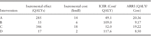
Figure 4 illustrates the mathematical programming solution using the diagrammatic approach employed by threshold searchers but also compatible with the questions addressed by threshold surveyors, based on the data in Table 1. Consider a decision maker with a budget of $20 million (E*) that is currently spent on interventions, A (incremental costs=$14 million, incremental effects=285 QALYs, ICER=49.1) and B (incremental costs=$6 million, incremental effects=55 QALYs, ICER=109). As we do not assume perfect divisibility, there is no MHG relevant to the decision maker. Instead we plot on the vertical axis the IHG (incremental benefit from the surveyors’ perspective) expressed as ARRI (QALYs per $1 million expenditure), which is the inverse of the ICER, in descending order. The ARRI of A and B are 20.36 and 9.17, respectively. The area under the IHG curve AA'BB' represents the total health gain from the $20 million budget and is given by the sum of the IHG for both interventions (or the ARRI multiplied by the expenditure on the intervention for each intervention and summed over both interventions). Total health gain for A and B is 340 QALYs.Footnote ³

Figure 4

Maximising efficiency under indivisibilities and non-constant returns to scale

Table 1

Incremental effects and incremental costs of interventions

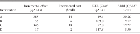
ICER=incremental cost-effectiveness ratio; ARRI=average rate of return on (additional) investment.

The right hand ‘panel’ on the diagram shows the corresponding IHGs (or benefits) for interventions C (incremental costs=$18 million, incremental effects=346 QALYs, ICER=52) and D (incremental costs=$2 million, incremental effects=17QALYs, ICER=117.6) not currently funded from the budget. Following Culyer et al. (Reference Culyer, McCabe, Briggs, Claxton, Buxton, Akehurst, Sculpher and Brazier2007), the ICER for current intervention B exceeds the ICER for new intervention C and so B should be replaced by C. However, the resources spent on B are insufficient to support C, so we cannot replace B by C. Hence, the ICER threshold approach says C should replace B, but there is no way of doing this using available resources without also cancelling A. However, the ICER threshold approach says A is preferred to C (it has a lower ICER than C) and hence should not be cancelled in order to provide resources for C.

The area under the IHG curve, CC'DD' in the right hand panel represents the health gain from spending the budget on new interventions C and D. This is 363 QALYs, greater than total health gains of the current interventions. This is seen by rotating the new interventions IHG curve CC'DD' around the vertical line at E* to give CFGJ in the current interventions panel. Although the ICER for A is less than the ICER for C and the ICER for B is less than the ICER for D, moving the entire budget from A and B and spending it on C and D would increase total health gain (and hence increase efficiency). Use of the ICER threshold rule and assumptions about incremental changes being simple aggregates of constant marginal changes leads the decision maker to choose the allocation of resources that produces less health gains.

Comparing areas under the IHG curves provides an unambiguous approach to determining whether introducing a new intervention represents an efficient resource allocation. Restricted (second best) solutions where full information on all possible programmes is not available have also been presented that generate unambiguous improvements in efficiency (Birch and Gafni, Reference Birch and Gafni1992; Sendi et al., Reference Sendi, Gafni and Birch2002; Gafni et al., Reference Gafni, Walter and Birch2013).