1 Introduction
Vortices are ubiquitous in nature. They are subject to various instabilities induced by interaction with their surroundings. In this work, we analyse the so-called curvature instability, which is a short-wavelength instability induced by the local curvature of the vortex. We provide theoretical predictions for a curved vortex when the underlying vortex structure is a Batchelor vortex (Gaussian axial velocity and axial vorticity). This work is the follow-up of Blanco-Rodríguez & Le Dizès (Reference Blanco-Rodríguez and Le Dizès2016), hereafter BRLD16, where another short-wavelength instability, the elliptic instability, was analysed using the same theoretical framework.
These two instabilities are different from the long-wavelength instabilities that occur in vortex pairs (Crow Reference Crow1970) and helical vortices (Widnall Reference Widnall1972; Quaranta, Bolnot & Leweke Reference Quaranta, Bolnot and Leweke2015). Their characteristics strongly depend on the internal vortex structure and their wavelength is of the order of the vortex core size. When the vortex is weakly deformed, both instabilities can be understood as a phenomenon of resonance between two (Kelvin) modes of the underlying vortex and a vortex correction. For the elliptic instability, the resonance occurs with a quadripolar correction generated by the background strain field (Moore & Saffman Reference Moore and Saffman1975), while for the curvature instability, it is associated with a dipolar correction created by the vortex curvature (Fukumoto & Hattori Reference Fukumoto and Hattori2005). Numerous works have concerned the elliptic instability in the context of straight vortices (Tsai & Widnall Reference Tsai and Widnall1976; Eloy & Le Dizès Reference Eloy and Le Dizès1999; Fabre & Jacquin Reference Fabre and Jacquin2004a ; Lacaze, Ryan & Le Dizès Reference Lacaze, Ryan and Le Dizès2007). The specific case of the curved Batchelor vortex has been analysed in BRLD16. In contrast to the elliptic instability, the curvature instability has only been considered for vortices with uniform vorticity (Fukumoto & Hattori Reference Fukumoto and Hattori2005; Hattori & Fukumoto Reference Hattori and Fukumoto2014).
Both elliptic and curvature instabilities have also been analysed using the local Lagrangian method popularized by Lifschitz & Hameiri (Reference Lifschitz and Hameiri1991) (see Bayly (Reference Bayly1986), Waleffe (Reference Waleffe1990) for the elliptic instability, Hattori & Fukumoto (Reference Hattori and Fukumoto2003, Reference Hattori and Fukumoto2009, Reference Hattori and Fukumoto2012) for the curvature instability). This method can be used to treat strongly deformed vortices, but it provides local information on a given streamline only. When the vortex is uniform, like the Rankine vortex, the local instability growth rate is also uniform. In that case, a connection can be made between the local results and the global results obtained by analysing the mode resonances (Waleffe Reference Waleffe1990; Eloy & Le Dizès Reference Eloy and Le Dizès2001; Fukumoto Reference Fukumoto2003; Hattori & Fukumoto Reference Hattori and Fukumoto2010, Reference Hattori and Fukumoto2014). Le Dizès & Laporte (Reference Le Dizès and Laporte2002) used the local prediction at the vortex centre to estimate the global growth rate of the elliptic instability in a non-uniform vortex. Although good agreement was demonstrated for the Lamb–Oseen vortex, no such link is expected in general.
The goal of the present work is to obtain global estimates for the curvature instability using the framework of Moore & Saffman (Reference Moore and Saffman1975) for the Batchelor vortex. Such an analysis was performed by Hattori & Fukumoto (Reference Hattori and Fukumoto2014) for a Rankine vortex. The passage from the Rankine vortex to the Batchelor vortex will turn out not to be trivial. The main reason comes from the different properties of the Kelvin modes in the two vortices. In smooth vortices, Kelvin modes are affected by the presence of critical layers (Le Dizès Reference Le Dizès2004), which introduce singularities and damping (Sipp & Jacquin Reference Sipp and Jacquin2003; Fabre, Sipp & Jacquin Reference Fabre, Sipp and Jacquin2006). These singularities have to be monitored and avoided in the complex plane to be able to obtain the properties of the Kelvin modes from the inviscid equations, as shown in Lacaze et al. (Reference Lacaze, Ryan and Le Dizès2007). In the present work, we shall also use the asymptotic theory of Le Dizès & Lacaze (Reference Le Dizès and Lacaze2005) to obtain an approximation of the Kelvin mode dispersion relation and analyse the condition of resonance.
The dipolar correction responsible of the curvature instability is also obtained by an asymptotic theory in the limit of small vortex core size (Callegari & Ting Reference Callegari and Ting1978). This correction appears as a first-order correction to the Batchelor vortex. The detail of the derivation can be found in Blanco-Rodríguez et al. (Reference Blanco-Rodríguez, Le Dizès, Selçuk, Delbende and Rossi2015). As for the elliptic instability, the coupling terms, as well as weak detuning and viscous effects, are computed using an orthogonality condition. The final result is an expression for the growth rate of a given resonant configuration close to the condition of resonance. Each resonant configuration provides a growth rate expression. We shall consider up to 50 resonant configurations to extract the most unstable one. This will allows us to obtain the curvature instability diagram as a function of the curvature ratio and the Reynolds number.
The paper is organized as follows. In § 2, the base flow and perturbation equations are provided. In § 3, the analysis leading to the growth rate expression of a resonant configuration is presented. The results for the Batchelor vortex are obtained in § 4. We first provide the characteristics of the resonant modes, then the stability diagrams for the Batchelor vortex for a few values of the axial flow parameter. Section 5 provides an application of the results to a vortex ring with and without swirl (axial flow). In that section, we analyse the competition of the curvature with the elliptic instability using the results of BRLD16. A numerical error affecting the strength of the elliptic instability has been found in BRLD16. It is corrected in a corrigendum which is presented in appendix D. Finally, § 6 gives a brief summary of the main results of the paper.
2 Problem formulation
2.1 Base flow
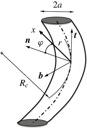
The first description of the base flow was provided by Callegari & Ting (Reference Callegari and Ting1978). Here, as in BRLD16, we mainly follow the presentation given in Blanco-Rodríguez et al. (Reference Blanco-Rodríguez, Le Dizès, Selçuk, Delbende and Rossi2015). The vortex is considered in the local Frenet frame (
 $\boldsymbol{t},\boldsymbol{n},\boldsymbol{b}$
) attached to the vortex centreline and moving with the structure. We assume that the vortex is concentrated (i.e. thin), which means that its core size
 $a$
is small compared with the local curvature radius
 $R_{c}$
of the vortex centreline and the shortest separation distance
 $\unicode[STIX]{x1D6FF}$
to other vortex structures. For simplicity, we consider a single small parameter
 $\unicode[STIX]{x1D700}=a/R_{c}$
, and assume that
 $\unicode[STIX]{x1D6FF}=O(R_{c})$
. The internal vortex dynamics is described using the ‘cylindrical’ coordinate system (
 $r,\unicode[STIX]{x1D711},s$
) constructed from the Frenet frame (see figure 1).
Sketch of the vortex structure and definition of the local Frenet frame (adapted from BRLD16).

The velocity–pressure field of the base flow is expanded in powers of
 $\unicode[STIX]{x1D700}$
as
 $\boldsymbol{U}=\boldsymbol{U}_{0}+\unicode[STIX]{x1D700}\boldsymbol{U}_{1}+\cdots \,$
. The leading-order contribution is the prescribed Batchelor vortex of velocity field
 $\boldsymbol{U}_{0}=(0,V^{(0)}(r),W^{(0)}(r),P^{(0)}(r))$
with
 $$\begin{eqnarray}V^{(0)}=\frac{1-\text{e}^{-r^{2}}}{r},\quad W^{(0)}=W_{0}\,\text{e}^{-r^{2}}.\end{eqnarray}$$
As in BRLD16, spatial and time scales have been non-dimensionalized using the core size
 $a$
and the maximum angular velocity of the vortex
 $\unicode[STIX]{x1D6FA}_{max}^{(0)}=\unicode[STIX]{x1D6E4}/(2\unicode[STIX]{x03C0}a^{2})$
,
 $\unicode[STIX]{x1D6E4}$
being the vortex circulation. The axial flow parameter
 $W_{0}$
is defined as the ratio
 $$\begin{eqnarray}W_{0}=\frac{W_{max}^{(0)}}{\unicode[STIX]{x1D6FA}_{max}^{(0)}a}.\end{eqnarray}$$
We assume that
 $W_{0}\leqslant 0.5$
, such that the vortex remains unaffected by the inviscid swirling jet instability (Mayer & Powell Reference Mayer and Powell1992). We also implicitly assume that the weak viscous instabilities occurring for small values of
 $W_{0}$
(Fabre & Jacquin Reference Fabre and Jacquin2004b
; Le Dizès & Fabre Reference Le Dizès and Fabre2007) remain negligible in the parameter regime that is considered. In the following, we shall also use the expression of the angular velocity
 $\unicode[STIX]{x1D6FA}^{(0)}(r)$
and vorticity
 $\unicode[STIX]{x1D701}^{(0)}(r)$
,
 $$\begin{eqnarray}\unicode[STIX]{x1D6FA}^{(0)}(r)=\frac{1-\text{e}^{-r^{2}}}{r^{2}},\quad \unicode[STIX]{x1D701}^{(0)}(r)=2\text{e}^{-r^{2}}.\end{eqnarray}$$
As explained by Blanco-Rodríguez et al. (Reference Blanco-Rodríguez, Le Dizès, Selçuk, Delbende and Rossi2015), the first-order correction is a dipolar field which can be written as
 $$\begin{eqnarray}\boldsymbol{U}_{1}\sim \unicode[STIX]{x1D700}Re\left(\boldsymbol{U}^{(1)}\text{e}^{\text{i}\unicode[STIX]{x1D711}}\right)=\frac{\unicode[STIX]{x1D700}}{2}\left(\begin{array}{@{}c@{}}\text{i}U^{(1)}(r)\\ V^{(1)}(r)\\ W^{(1)}(r)\\ P^{(1)}(r)\end{array}\right)\text{e}^{\text{i}\unicode[STIX]{x1D711}}+\text{c.c.},\end{eqnarray}$$
where expressions for
 $U^{(1)}$
,
 $V^{(1)}$
,
 $W^{(1)}$
and
 $P^{(1)}$
are provided in appendix A. It is worth emphasizing that these expressions only depend on the local characteristics of the vortex at leading order. In particular, they do not depend on the local torsion. For helices, torsion as well as the Coriolis effects associated with the change of frame appear at second order (Hattori & Fukumoto Reference Hattori and Fukumoto2009). The above expression then describes the internal structure of both helices and rings up to the order
 $\unicode[STIX]{x1D700}$
. This contrasts with the quadripolar correction responsible for the elliptic instability which appears at second order. This quadripolar correction varies according to the global vortex geometry and is different for rings and helices even if they have the same local curvature.
2.2 Perturbation equations
The perturbation equations are obtained by linearizing the governing equations around the base flow
 $\boldsymbol{U}=\boldsymbol{U}_{0}+\unicode[STIX]{x1D700}\boldsymbol{U}_{1}+\cdots \,$
. As shown in BRLD16, if the perturbation velocity–pressure field is written as
 $\boldsymbol{u}=(-\text{i}u,v,w,p)$
, we obtain up to
 $o(\unicode[STIX]{x1D700})$
terms a system of the form
 $$\begin{eqnarray}\left(\text{i}\unicode[STIX]{x2202}_{t}\boldsymbol{I}+\text{i}\unicode[STIX]{x2202}_{s}\boldsymbol{P}+\boldsymbol{M}\right)\boldsymbol{u}=\unicode[STIX]{x1D700}\left(\text{e}^{\text{i}\unicode[STIX]{x1D711}}\boldsymbol{N}_{+}^{(1)}+\text{e}^{-\text{i}\unicode[STIX]{x1D711}}\boldsymbol{N}_{-}^{(1)}\right)\boldsymbol{u}+\displaystyle \frac{\text{i}}{\mathit{Re}}\boldsymbol{V}\boldsymbol{u},\end{eqnarray}$$
where the operators
 $\boldsymbol{I}$
,
 $\boldsymbol{P}$
,
 $\boldsymbol{M}=\boldsymbol{M}(-\text{i}\unicode[STIX]{x2202}_{\unicode[STIX]{x1D711}})$
,
 $\boldsymbol{N}_{\pm }^{(1)}=\boldsymbol{N}_{\pm }^{(1)}(-\text{i}\unicode[STIX]{x2202}_{\unicode[STIX]{x1D711}},-\text{i}\unicode[STIX]{x2202}_{s})$
,
 $\boldsymbol{V}=\boldsymbol{V}(-\text{i}\unicode[STIX]{x2202}_{\unicode[STIX]{x1D711}},-\text{i}\unicode[STIX]{x2202}_{s})$
are defined in appendix B.
The left-hand side corresponds to the inviscid perturbation equations of the undeformed Batchelor vortex. The first term on the right-hand side is responsible for the curvature instability, while the second term accounts for the viscous effects on the perturbations. By introducing viscous effects in this equation, we implicitly assume that the Reynolds number
 $$\begin{eqnarray}\mathit{Re}=\frac{\unicode[STIX]{x1D6FA}_{max}^{(0)}a^{2}}{\unicode[STIX]{x1D708}}=\frac{\unicode[STIX]{x1D6E4}}{2\unicode[STIX]{x03C0}\unicode[STIX]{x1D708}},\end{eqnarray}$$
with
 $\unicode[STIX]{x1D708}$
the kinematic viscosity, is of order
 $1/\unicode[STIX]{x1D700}$
.
3 Instability description
3.1 Curvature instability mechanism
The mechanism of the curvature instability is similar to that of the elliptic instability. The instability results from a resonant coupling of two Kelvin modes of the undeformed axisymmetric vortex with non-axisymmetric corrections. Two Kelvin modes of characteristics
 $(\unicode[STIX]{x1D714}_{A},k_{A},m_{A})$
and
 $(\unicode[STIX]{x1D714}_{B},k_{B},m_{B})$
are resonantly coupled via the dipolar correction if they satisfy the condition of resonance (assuming
 $m_{A}<m_{B}$
)
 $$\begin{eqnarray}\unicode[STIX]{x1D714}_{A}=\unicode[STIX]{x1D714}_{B},\quad k_{A}=k_{B},\quad m_{A}=m_{B}-1.\end{eqnarray}$$
Fukumoto (Reference Fukumoto2003) further demonstrated that the coupling is destabilizing only if the energies of the modes are opposite or if the frequency vanishes. This leads to a growth of the Kelvin mode combination with a maximum growth rate scaling as
 $\unicode[STIX]{x1D700}$
.
3.2 Formal derivation of the growth rate formula
For each resonant configuration, a growth rate expression can be obtained from an orthogonality condition, as we did for the elliptic instability (see BRLD16). We consider a combination of two Kelvin modes of azimuthal wavenumbers
 $m_{A}$
and
 $m_{B}=m_{A}+1$
close to the their condition of resonance (3.1),
 $$\begin{eqnarray}\boldsymbol{u}=\left(A\tilde{\boldsymbol{u}}_{A}(r)\,\text{e}^{\text{i}m_{A}\unicode[STIX]{x1D711}}+B\tilde{\boldsymbol{u}}_{B}(r)\,\text{e}^{\text{i}m_{B}\unicode[STIX]{x1D711}}\right)\,\text{e}^{\text{i}ks-\text{i}\unicode[STIX]{x1D714}t},\end{eqnarray}$$
where
 $k$
is close to
 $k_{A}=k_{B}=k_{c}$
, and
 $\unicode[STIX]{x1D714}$
is close to
 $\unicode[STIX]{x1D714}_{A}=\unicode[STIX]{x1D714}_{c}$
and
 $\unicode[STIX]{x1D714}_{B}=\unicode[STIX]{x1D714}_{c}+\text{i}\,\text{Im}(\unicode[STIX]{x1D714}_{B})$
. We assume that the resonance is not perfect. The mode B will exhibit a weak critical layer damping given by
 $\text{Im}(\unicode[STIX]{x1D714}_{B})$
(imaginary part of
 $\unicode[STIX]{x1D714}_{B}$
). The functions
 $\tilde{\boldsymbol{u}}_{A}(r)$
and
 $\tilde{\boldsymbol{u}}_{B}(r)$
are the eigenfunctions of the Kelvin modes which satisfy
 $$\begin{eqnarray}\displaystyle & \displaystyle \left(\unicode[STIX]{x1D714}_{A}\boldsymbol{I}-k_{A}\boldsymbol{P}+\boldsymbol{M}(m_{A})\right)\tilde{\boldsymbol{u}}_{A}=0, & \displaystyle\end{eqnarray}$$
 $$\begin{eqnarray}\displaystyle & \displaystyle \left(\unicode[STIX]{x1D714}_{B}\boldsymbol{I}-k_{B}\boldsymbol{P}+\boldsymbol{M}(m_{B})\right)\tilde{\boldsymbol{u}}_{B}=0, & \displaystyle\end{eqnarray}$$
with a prescribed normalization
 $$\begin{eqnarray}\tilde{p}_{A}\;\underset{r\,\rightarrow \,0}{{\sim}}\;r^{|m_{A}|},\quad \tilde{p}_{B}\;\underset{r\,\rightarrow \,0}{{\sim}}\;r^{|m_{B}|}.\end{eqnarray}$$
If we plug (3.2) into (2.5), we obtain for the components proportional to
 $\text{e}^{\text{i}m_{A}\unicode[STIX]{x1D711}}$
and
 $\text{e}^{\text{i}m_{B}\unicode[STIX]{x1D711}}$
 $$\begin{eqnarray}\displaystyle & \displaystyle A\left(\unicode[STIX]{x1D714}\boldsymbol{I}-k\boldsymbol{P}+\boldsymbol{M}(m_{A})-\displaystyle \frac{\text{i}}{\mathit{Re}}\boldsymbol{V}(m_{A},k)\right)\tilde{\boldsymbol{u}}_{A}=B\unicode[STIX]{x1D700}\boldsymbol{N}_{-}^{(1)}(m_{B},k)\tilde{\boldsymbol{u}}_{B}, & \displaystyle\end{eqnarray}$$
 $$\begin{eqnarray}\displaystyle & \displaystyle B\left(\unicode[STIX]{x1D714}\boldsymbol{I}-k\boldsymbol{P}+\boldsymbol{M}(m_{B})-\displaystyle \frac{\text{i}}{\mathit{Re}}\boldsymbol{V}(m_{B},k)\right)\tilde{\boldsymbol{u}}_{B}=A\unicode[STIX]{x1D700}\boldsymbol{N}_{+}^{(1)}(m_{A},k)\tilde{\boldsymbol{u}}_{A}. & \displaystyle\end{eqnarray}$$
Relations between the amplitudes
 $A$
and
 $B$
are obtained by projecting these equations onto the subspace of the adjoint Kelvin modes. We define the adjoint eigenfunctions
 $\tilde{\boldsymbol{u}}_{A}^{\dagger }$
and
 $\tilde{\boldsymbol{u}}_{B}^{\dagger }$
of the Kelvin modes as the solutions to the adjoint equations of (3.3)–(3.4) with respect to the scalar product
 $$\begin{eqnarray}\langle \boldsymbol{u}_{1},\boldsymbol{u}_{2}\rangle =\int _{0}^{\infty }\boldsymbol{u}_{1}^{\star }\boldsymbol{\cdot }\boldsymbol{u}_{2}\,r\,\text{d}r=\int _{0}^{\infty }\left(u_{1}^{\star }u_{2}+v_{1}^{\star }v_{2}+w_{1}^{\star }w_{2}+p_{1}^{\star }p_{2}\right)r\,\text{d}r.\end{eqnarray}$$
We then obtain
 $$\begin{eqnarray}\left(\unicode[STIX]{x1D714}-\unicode[STIX]{x1D714}_{c}-Q_{A}(k-k_{c})-\text{i}\displaystyle \frac{V_{A}}{\mathit{Re}}\right)A=\unicode[STIX]{x1D700}C_{AB}B,\end{eqnarray}$$
 $$\begin{eqnarray}\left(\unicode[STIX]{x1D714}-\unicode[STIX]{x1D714}_{c}-\text{i}\,\text{Im}(\unicode[STIX]{x1D714}_{B})-Q_{B}(k-k_{c})-\text{i}\displaystyle \frac{V_{B}}{\mathit{Re}}\right)B=\unicode[STIX]{x1D700}C_{BA}A,\end{eqnarray}$$
where the coefficients of these equations are given by
 $$\begin{eqnarray}Q_{A}=\displaystyle \frac{\langle \tilde{\boldsymbol{u}}_{A}^{\dagger },\boldsymbol{P}\,\tilde{\boldsymbol{u}}_{A}\rangle }{\langle \tilde{\boldsymbol{u}}_{A}^{\dagger },\boldsymbol{I}\,\tilde{\boldsymbol{u}}_{A}\rangle },\quad Q_{B}=\displaystyle \frac{\langle \tilde{\boldsymbol{u}}_{B}^{\dagger },\boldsymbol{P}\,\tilde{\boldsymbol{u}}_{B}\rangle }{\langle \tilde{\boldsymbol{u}}_{B}^{\dagger },\boldsymbol{I}\,\tilde{\boldsymbol{u}}_{B}\rangle },\end{eqnarray}$$
 $$\begin{eqnarray}V_{A}=\displaystyle \frac{\langle \tilde{\boldsymbol{u}}_{A}^{\dagger },\boldsymbol{V}\,\tilde{\boldsymbol{u}}_{A}\rangle }{\langle \tilde{\boldsymbol{u}}_{A}^{\dagger },\boldsymbol{I}\,\tilde{\boldsymbol{u}}_{A}\rangle },\quad V_{B}=\displaystyle \frac{\langle \tilde{\boldsymbol{u}}_{B}^{\dagger },\boldsymbol{V}\,\tilde{\boldsymbol{u}}_{B}\rangle }{\langle \tilde{\boldsymbol{u}}_{B}^{\dagger },\boldsymbol{I}\,\tilde{\boldsymbol{u}}_{B}\rangle },\end{eqnarray}$$
 $$\begin{eqnarray}C_{AB}=\displaystyle \frac{\langle \tilde{\boldsymbol{u}}_{A}^{\dagger },\boldsymbol{N}_{+}^{(1)}(m_{B},k_{B})\,\tilde{\boldsymbol{u}}_{B}\rangle }{\langle \tilde{\boldsymbol{u}}_{A}^{\dagger },\boldsymbol{I}\,\tilde{\boldsymbol{u}}_{A}\rangle },\quad C_{BA}=\displaystyle \frac{\langle \tilde{\boldsymbol{u}}_{B}^{\dagger },\boldsymbol{N}_{-}^{(1)}(m_{A},k_{A})\,\tilde{\boldsymbol{u}}_{A}\rangle }{\langle \tilde{\boldsymbol{u}}_{B}^{\dagger },\boldsymbol{I}\,\tilde{\boldsymbol{u}}_{B}\rangle }.\end{eqnarray}$$
The formula for the complex frequency
 $\unicode[STIX]{x1D714}$
is then finally given by
 $$\begin{eqnarray}\left(\unicode[STIX]{x1D714}-\unicode[STIX]{x1D714}_{c}-\text{i}~\text{Im}(\unicode[STIX]{x1D714}_{B})-Q_{B}(k-k_{c})-\text{i}\displaystyle \frac{V_{B}}{\mathit{Re}}\right)\left(\unicode[STIX]{x1D714}-\unicode[STIX]{x1D714}_{c}-Q_{A}(k-k_{c})-\text{i}\displaystyle \frac{V_{A}}{\mathit{Re}}\right)=-\unicode[STIX]{x1D700}^{2}N^{2},\end{eqnarray}$$
with
 $$\begin{eqnarray}N=\sqrt{-C_{AB}C_{BA}}~.\end{eqnarray}$$
The right-hand side of (3.14) represents the coupling terms responsible for the curvature instability. The left-hand side of (3.14) gives the dispersion relation of each Kelvin mode close to the resonant point. It is important to mention that none of the coefficients
 $Q_{A}$
,
 $Q_{B}$
,
 $V_{A}$
,
 $V_{B}$
and
 $N$
depend on the normalization chosen for the Kelvin modes.
4 Instability results for the Batchelor vortex profile
4.1 Resonant Kelvin modes
The main difficulty of the analysis is to determine the Kelvin modes that satisfy the condition of resonance (3.1). A similar problem was already addressed in Lacaze et al. (Reference Lacaze, Ryan and Le Dizès2007). The Kelvin modes are here defined from the inviscid equations. Two kinds of Kelvin modes are found to exist: the regular and neutral Kelvin modes, which can easily be obtained by integrating the inviscid perturbation equations in the physical domain, and the singular and damped Kelvin modes, which require a particular monitoring of the singularities of the perturbation equations in the complex plane. We shall see below that the condition of resonance always involves a singular mode.
The singularities of the inviscid perturbation equations are the critical points
 $r_{c}$
where
 $\unicode[STIX]{x1D714}-kW^{(0)}(r_{c})-m\unicode[STIX]{x1D6FA}^{(0)}(r_{c})=0$
. When
 $\text{Im}(\unicode[STIX]{x1D714})>0$
, these singularities are in the complex plane and do not affect the solution in the physical domain (real
 $r$
). However, one of these critical points may cross the real axis when
 $\text{Im}(\unicode[STIX]{x1D714})$
becomes negative. As explained in Le Dizès (Reference Le Dizès2004), the inviscid equations must in that case be integrated on a contour in the complex
 $r$
plane that avoids the critical point from below (respectively above) if the critical point has moved in the lower (respectively upper) part of the complex plane. On such a contour, the solution remains regular and fully prescribed by the inviscid equations. On the real axis, the inviscid solution is, however, not regular anymore. As illustrated in Fabre et al. (Reference Fabre, Sipp and Jacquin2006), it no longer represents the vanishing viscosity limit of a viscous solution in a large interval of the physical domain. The Kelvin mode formed by the contour deformation technique is damped and singular. The inviscid frequency of the mode then possesses a negative imaginary part, which corresponds to what we call the critical layer damping rate. By definition, the critical layer damping rate is independent of viscosity.
A mode cannot be involved in a resonance if it is damped too much. In the asymptotic framework, the growth rate associated with the resonance is expected to be
 $O(\unicode[STIX]{x1D700})$
, so the damping rate of the modes should a priori be asymptotically small of order
 $\unicode[STIX]{x1D700}$
. However, in practice, we shall consider values of
 $\unicode[STIX]{x1D700}$
up to
 $0.2$
, and the maximum growth rate will turn out to be approximately
 $0.05\,\unicode[STIX]{x1D700}$
. We shall then discard all the modes with a damping rate whose absolute value exceeds
 $0.01$
.
4.1.1 Predictions from the large-
 $k$
asymptotic analysis

Le Dizès & Lacaze (Reference Le Dizès and Lacaze2005) showed that information on the spectrum of the Kelvin modes can be obtained using a large-
 $k$
asymptotic analysis. They applied their theory to the Batchelor vortex and were able to categorize the neutral Kelvin modes into four different types: regular core modes, singular core modes, regular ring modes and singular ring modes. For each
 $m$
, they provided the region of existence of each type of mode in a (
 $kW_{0},\unicode[STIX]{x1D714}$
) plane. The energy of the waves can also be deduced from the asymptotic expression of the dispersion relation, as shown in Le Dizès (Reference Le Dizès2008). It is immediately found that regular core modes and regular ring modes are always of negative energy, while singular modes have positive energy.
Prediction from the large-
 $k$
asymptotic analysis of the domains of parameters in the (
 $kW_{0},\unicode[STIX]{x1D714}$
) plane where resonance between two Kelvin modes
 $(m_{A},m_{A}+1)$
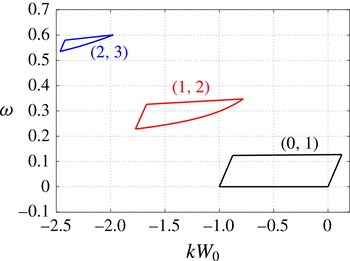
is possible. Only positive frequencies are considered. A symmetrical plot is obtained for negative frequencies.

The condition of resonance can then easily be analysed. One just needs to superimpose the domains of existence of each pair of modes of azimuthal wavenumbers
 $m$
and
 $m+1$
to find the regions of possible resonance. The final result is summarized in figure 2. For positive frequencies, only three different regions are obtained corresponding to
 $(m_{A},m_{B})=(0,1)$
,
 $(1,2)$
and
 $(2,3)$
(Negative frequencies are obtained by symmetry changing
 $m\rightarrow -m$
and
 $k\rightarrow -k$
.) No intersection of the domains of existence of the modes
 $m$
and
 $m+1$
is obtained for
 $m$
larger than
 $2$
. In each region of figure 2, we always find that the mode
 $A$
is a regular core mode of negative energy, while the mode
 $B$
is a singular core mode of positive energy. Each branch crossing is therefore expected to provide an instability.
As shown in Le Dizès & Lacaze (Reference Le Dizès and Lacaze2005), both types of core modes have an asymptotic dispersion relation of the form
 $$\begin{eqnarray}k\int _{0}^{r_{t}}\frac{\sqrt{\unicode[STIX]{x0394}(r)}}{\unicode[STIX]{x1D6F7}(r)}\,\text{d}r=\left(|m|+2l\right)\frac{\unicode[STIX]{x03C0}}{2}\quad l=0,1,2,\ldots ,\end{eqnarray}$$
where
 $$\begin{eqnarray}\displaystyle & \displaystyle \unicode[STIX]{x0394}(r)=2\unicode[STIX]{x1D6FA}^{(0)}(r)\unicode[STIX]{x1D701}^{(0)}(r)-\unicode[STIX]{x1D6F7}^{2}(r), & \displaystyle\end{eqnarray}$$
 $$\begin{eqnarray}\displaystyle & \displaystyle \unicode[STIX]{x1D6F7}(r)=\unicode[STIX]{x1D714}-m\unicode[STIX]{x1D6FA}^{(0)}(r)-kW^{(0)}(r) & \displaystyle\end{eqnarray}$$
and
 $r_{t}$
is a turning point defined by
 $\unicode[STIX]{x0394}(r_{t})=0$
. The integer
 $l$
is a branch label which measures the number of oscillations of the mode in the vortex core. The larger
 $l$
is, the more oscillating the mode is.
Singular modes differ from regular modes by the presence of a critical point
 $r_{c}>r_{t}$
where
 $\unicode[STIX]{x1D6F7}(r_{c})=0$
in their radial structure. In the large-
 $k$
asymptotic description, this critical point does not create any damping at leading order. However, it makes the eigenfunction singular. It will justify the use of a complex integration path in the numerical resolution of the mode.
4.1.2 Numerical determination of the Kelvin modes
The characteristics of the resonant modes are obtained by integrating (3.3)–(3.4) numerically. The numerical code is based on a Chebyshev spectral collocation method, essentially identical to that used in Fabre & Jacquin (Reference Fabre and Jacquin2004b ).
The eigenvalue problem is solved in a Chebyshev domain
 $(-1,1)$
on
 $2(N+1)$
nodes, which is mapped onto a line in the complex-
 $r$
plane using the mapping
 $$\begin{eqnarray}r(x;A_{c},\unicode[STIX]{x1D703}_{c})=A_{c}\,\tanh (x)\,\text{e}^{\text{i}\,\unicode[STIX]{x1D703}_{c}},\end{eqnarray}$$
where
 $A_{c}$
is a parameter close to 1 that controls the spreading of the collocation points and
 $\unicode[STIX]{x1D703}_{c}$
is the small inclination angle of the path in the complex-
 $r$
plane. We typically take
 $\unicode[STIX]{x1D703}_{c}\approx \unicode[STIX]{x03C0}/10$
, such that the critical point of the singular mode is avoided. As in Fabre & Jacquin (Reference Fabre and Jacquin2004b
), we take advantage of the parity properties of the eigenfunctions by expressing for odd
 $m$
(respectively even
 $m$
),
 $\tilde{w}$
and
 $\tilde{p}$
on odd polynomials (respectively even) and
 $\tilde{u}$
and
 $\tilde{v}$
on even polynomials (respectively odd). This leads to a discretized eigenvalue problem of order
 $4N$
, which is solved using a global eigenvalue method. We also use an Arnoldi algorithm in order to follow specific eigenvalues and easily find the condition of resonance. In most computations, the value
 $N=200$
was found to be adequate.
This collocation method was also used to determine the adjoint modes and compute the integrals that define the coefficients in the growth rate equation (3.14).
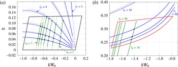
Typical results for the eigenvalues are shown in figure 3. In this figure, we compare the numerical results with the theoretical formula (4.1). The good agreement demonstrates the usefulness of the asymptotic approach to obtain valuable estimates for the condition of resonance.
Analysis of the branch crossing for the Batchelor vortex at
 $W_{0}=0.2$
. Plot of
 $\text{Re}(\unicode[STIX]{x1D714})$
versus
 $kW_{0}$
of the first branches of the Kelvin modes of azimuthal wavenumber
 $m_{A}$
(in blue) and
 $m_{B}=m_{A}+1$
(in green) for (a)
 $(m_{A},m_{B})=(0,1)$
and (b)
 $(m_{A},m_{B})=(1,2)$
. The branch labels are also indicated. The solid lines show numerical results and the dashed lines show large-
 $k$
asymptotic predictions. The domains shown in figure 2 where branch crossings are expected have also been indicated.

4.2 Stability diagram
4.2.1 Lamb–Oseen vortex
In this section, we assume that there is no axial flow. The underlying vortex is then a Lamb–Oseen vortex. For this vortex, Kelvin mode properties have been documented in Le Dizès & Lacaze (Reference Le Dizès and Lacaze2005) and Fabre et al. (Reference Fabre, Sipp and Jacquin2006) for
 $m=0$
, 1, 2, 3. It was shown that the singular core modes become strongly damped as soon as the critical layer singularity moves in the vortex core. This gives a constraint on the frequency of the mode
 $B$
which has to be small. As a consequence, we immediately see that the only modes
 $(m_{A},m_{B})$
that can possibly resonate are the modes
 $(m_{A},m_{B})=(0,1)$
. Moreover, the constraint on the frequency implies that only large branch labels of the mode
 $m_{A}=0$
will be able to resonate with a weakly damped mode
 $m_{B}=1$
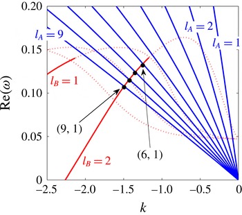
. In figure 4, we show the crossing of the first
 $m_{A}=0$
and
 $m_{B}=1$
branches in the
 $(k,\unicode[STIX]{x1D714})$
plane. Only the modes with a damping rate smaller (in absolute value) than 0.01 are plotted with solid lines. We observe that the branch label of the
 $m_{A}=0$
modes must be 6 or larger to cross the first
 $m_{B}=1$
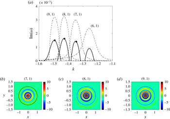
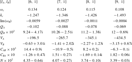
branch in the part where it is only weakly damped. The characteristics of these first resonance points are given in table 1 (appendix C). We also give in this table the values of the coefficients of (3.14) at each resonant point. For each resonant configuration, we can then plot the growth rate
 $\text{Im}(\unicode[STIX]{x1D714})$
of the curvature instability as a function of the wavenumber
 $k$
for any
 $\mathit{Re}$
and
 $\unicode[STIX]{x1D700}$
. An example of such a plot is provided in figure 5. In this figure, we have plotted only the first four resonant configurations. Other configurations have been computed corresponding to labels
 $(2,6),(2,7)$
, etc., but their growth rates were found to be much weaker for
 $\mathit{Re}\leqslant 10^{5}$
. The spatial structures of the most unstable resonant configurations are also given in figure 5. We have plotted the vorticity contours for a particular phase that maximizes the relative amplitude of the Kelvin mode
 $m_{A}=0$
. This mode is then clearly visible in each case. If we had chosen a phase such that
 $\text{e}^{\text{i}ks-\text{i}\unicode[STIX]{x1D714}t}=\text{i}$
, we would have seen the mode
 $m_{B}=1$
only.
Frequency versus wavenumber of the Kelvin modes of the Lamb–Oseen vortex for
 $m_{A}=0$
(blue) and
 $m_{B}=1$
(red) in the frequency–wavenumber domain where resonance exists. The real part of the frequency is plotted with solid lines when
 $|\text{Im}(\unicode[STIX]{x1D714})|<0.01$
(neutral or weakly damped modes) and with dotted lines when
 $|\text{Im}(\unicode[STIX]{x1D714})|>0.01$
(strongly damped modes).

(a) Temporal growth rate of the curvature instability as a function of the axial wavenumber for the Lamb–Oseen vortex (
 $W_{0}=0$
) at
 $\unicode[STIX]{x1D700}=0.1$
,
 $\mathit{Re}=\infty$
(dashed line) and
 $\mathit{Re}=10^{5}$
. The label
 $[l_{A},l_{B}]$
corresponds to the branch indices of the resonant configuration. It means that the resonant configuration is formed of the
 $l_{A}$
th branch of the Kelvin mode
 $m_{A}=0$
and the
 $l_{B}$
th branch of the Kelvin mode
 $m_{B}=1$
. (b–d) Vorticity contours in an
 $(x,y)$
cross-section of modes
 $(7,1)$
,
 $(8,1)$
and
 $(9,1)$
for the parameters indicated by a star in (a) (that is, at
 $k=k_{c}$
). The vorticity is defined by (3.2) at a time
 $t$
and location
 $s$
such that
 $\text{e}^{\text{i}ks-\text{i}\unicode[STIX]{x1D714}t}=1$
with
 $A=1$
. The black circle indicates the vortex core radius.

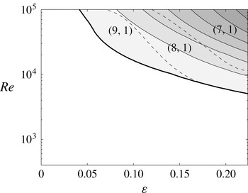
We have systematically computed the maximum growth rate and obtained the most unstable mode characteristics for all
 $\unicode[STIX]{x1D700}\leqslant 0.22$
and
 $\mathit{Re}\leqslant 10^{5}$
. The result is displayed in figure 6, where the maximum growth rate is shown in the
 $(\unicode[STIX]{x1D700},\mathit{Re})$
plane. The labels of the most unstable configurations are also shown in this plot. We can note that only three resonant configurations can become the most unstable corresponding to the crossing of the first branch of the Kelvin mode
 $m_{B}=1$
with the seventh–ninth branches of the Kelvin mode
 $m_{A}=0$
. In particular, the resonant configuration
 $(6,1)$
observed in figure 5 never becomes the most unstable configuration although this configuration possesses the largest coupling coefficient
 $N$
(see table 1 in appendix C). This is directly related to the property mentioned above: the critical layer damping rate
 $\text{Im}(\unicode[STIX]{x1D714}_{B})$
of the mode
 $m_{B}=1$
is too large.
Maximum growth rate contour of the curvature instability in the (
 $\unicode[STIX]{x1D700}$
,
 $\mathit{Re}$
) plane for the Lamb–Oseen vortex (
 $W_{0}=0$
). The contours are every 0.001. The thick solid line indicates the marginal stability curve. The dashed lines are the parameter boundaries where the most unstable configuration indicated by the label
 $[l_{A},l_{B}]$
changes.

Figure 6 provides the stability diagram of the Lamb–Oseen vortex with respect to the curvature instability. It is important to emphasize the large value of the Reynolds number needed for instability. Even for a value as large as
 $\unicode[STIX]{x1D700}=0.2$
, the critical Reynolds number for instability is
 $\mathit{Re}_{c}\approx 6000$
. We shall see in the next section that axial flow will strongly decrease this value.
4.2.2 Effects of the axial flow
The characteristics of the Kelvin modes strongly vary with the parameter
 $W_{0}$
. Additional branch crossings involving smaller branch labels are obtained as
 $W_{0}$
increases. As explained in the previous section, resonances between
 $m_{A}=1$
and
 $m_{B}=2$
, as well as between
 $m_{A}=2$
and
 $m_{B}=3$
, become a priori possible (see figure 2). However, they involve very high branch labels, which implies that they never become the most unstable modes for moderate Reynolds numbers (
 $\mathit{Re}\leqslant 10^{5}$
).
For the parameters
 $W_{0}=0.1,0.2,0.3,0.4$
and 0.5, we have considered the crossing points of the first seven branches of the Kelvin modes
 $m_{A}=0$
and
 $m_{B}=1$
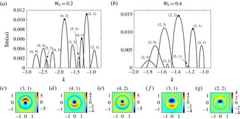
. Each crossing point corresponds to a mode resonance. At each crossing point, we have computed the coefficients of the growth rate expression. In figure 7, we have plotted the growth rate curves obtained from (3.14) for
 $W_{0}=0.2$
and 0.4, and for
 $\unicode[STIX]{x1D700}=0.2$
and
 $\mathit{Re}=5000$
. In contrast to the Lamb–Oseen vortex, more resonant configurations can now become unstable. Moreover, they involve smaller branch labels. The spatial structure of the main resonant configurations have also been provided in figure 7 for this set of parameters. As in figure 5, we have plotted the vorticity contour for a particular phase that maximizes the relative amplitude of the Kelvin mode
 $m_{A}=0$
. It should be noted that the spatial structure of the resonant mode
 $(3,1)$
is different for
 $W_{0}=0.2$
and
 $W_{0}=0.4$
. This difference is not only associated with the different values of the coefficient
 $B/A$
obtained from (3.6), but also with an effect of
 $W_{0}$
on the Kelvin modes.
(a,b) Temporal growth rate of the curvature instability as a function of the axial wavenumber for the Batchelor vortex at
 $\unicode[STIX]{x1D700}=0.2$
and
 $\mathit{Re}=5000$
for
 $W_{0}=0.2$
(a) and
 $W_{0}=0.4$
(b). (c–g) Vorticity contours in an
 $(x,y)$
cross-section of modes
 $(3,1)$
,
 $(4,1)$
and
 $(4,2)$
for
 $W_{0}=0.2$
(c,d,e) and modes (3, 1) and (2, 2) for
 $W_{0}=0.4$
(f,g). See the caption to figure 5 for more information.

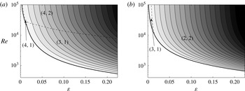
If we take the maximum value of the growth rate over all possible
 $k$
for each
 $\unicode[STIX]{x1D700}$
and
 $\mathit{Re}$
, we obtain the plots shown in figure 8. The same colourmap and contour levels have been used as in figure 6 for comparison. We clearly see that the growth rates are larger in the presence of axial flow. The region of instability is also much larger. In these plots, we have indicated the labels of the most unstable modes. As for the Lamb–Oseen vortex, the most unstable configuration changes as
 $\unicode[STIX]{x1D700}$
or
 $\mathit{Re}$
varies. However, the branch labels of the Kelvin modes are now smaller in the presence of axial flow. This property explains in part the larger growth rates of the configurations with jets. Indeed, the viscous damping of the modes with the smallest labels is the weakest. The impact of viscosity is therefore weaker on these modes. However, the resonant configurations with the smallest labels are not necessarily the most unstable because they may also exhibit a larger critical layer damping, or a smaller coupling coefficient
 $N$
(see (3.14)).
Maximum growth rate contours of the curvature instability in the (
 $\unicode[STIX]{x1D700}$
,
 $\mathit{Re}$
) plane for the Batchelor vortex for (a)
 $W_{0}=0.2$
and (b)
 $W_{0}=0.4$
. See the caption to figure 6.

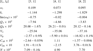
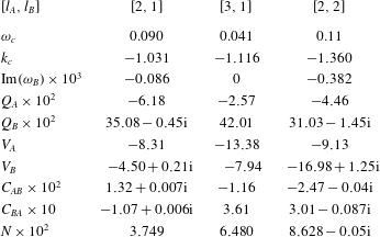
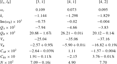
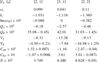
In tables 2 and 3 of appendix C, we have provided the characteristics of the main resonant configurations for
 $W_{0}=0.2$
and
 $W_{0}=0.4$
. The data for the other resonant configurations and for other values of
 $W_{0}$
are available as supplementary material at https://doi.org/10.1017/jfm.2017.34.
5 Competition with the elliptic instability in a vortex ring
The results obtained in § 4 can readily be applied to a vortex ring by using
 $\unicode[STIX]{x1D700}=a/R$
, where
 $R$
is the radius of the ring and
 $a$
is the core radius.
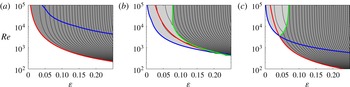
Maximum growth rate contours of short-wavelength instabilities (curvature instability and elliptic instability) in a vortex ring with a Batchelor vortex profile in the (
 $\unicode[STIX]{x1D700}=a/R$
,
 $\mathit{Re}$
) plane for (a)
 $W_{0}=0$
, (b)
 $W_{0}=0.2$
and (c)
 $W_{0}=0.4$
. The contours are every 0.002. The blue line shows the marginal curve of the curvature instability (
 $\text{Im}(\unicode[STIX]{x1D714}_{curv})=0$
), the red line shows the marginal curve of the elliptic instability (
 $\text{Im}(\unicode[STIX]{x1D714}_{ellip})=0$
) and the green line shows the line of equal dominance of both instabilities (
 $\text{Im}(\unicode[STIX]{x1D714}_{ellip})=\text{Im}(\unicode[STIX]{x1D714}_{curv})$
). Elliptic instability dominates curvature instability in the dark grey region.

As first shown by Widnall, Bliss & Tsai (Reference Widnall, Bliss and Tsai1974), a vortex ring is also subject to the elliptic instability. This instability appears at the order
 $\unicode[STIX]{x1D700}^{2}$
, so it is a priori smaller. However, the short-wavelength instability observed experimentally in a vortex ring without swirl has always been attributed to the elliptic instability (see the review by Shariff & Leonard Reference Shariff and Leonard1992). It is therefore natural to provide a more precise comparison of the growth rates of the two instabilities.
In BRLD16, we obtained theoretical predictions for the elliptic instability in a vortex ring with a Batchelor profile. As for the curvature instability, growth rate contour plots can be obtained for the elliptic instability in an
 $(\unicode[STIX]{x1D700},\mathit{Re})$
plane using the data of this paper. It should be noted that an error of a factor 2 was found in some of the coefficients of the elliptic instability growth rate formula. This error, which is corrected in appendix D, does not affect the main conclusion of this paper but modifies the relative importance of the elliptic instability with respect to the curvature instability.
The comparison of the elliptic instability with the curvature instability is shown in figure 9 for three values of the axial flow parameter (
 $W_{0}=0,0.2,0.4$
). In this figure, we have plotted the largest values of both instability growth rates in the
 $(\unicode[STIX]{x1D700},\mathit{Re})$
plane. We have also indicated where each instability appears and becomes dominant over the other one. Interestingly, we observe that, depending on the value of
 $W_{0}$
, the region of dominance of the curvature instability changes. For the case without axial flow (figure 9
a), the elliptic instability domain is larger than the curvature instability domain and the elliptic instability is always the dominant instability. For the other two cases,
 $W_{0}=0.2$
and
 $W_{0}=0.4$
, the situation is different: there is a balance between the two instabilities. For both cases, the curvature instability is dominant over the elliptic instability for small
 $\unicode[STIX]{x1D700}$
while it is the opposite for large
 $\unicode[STIX]{x1D700}$
. However, there are some differences between the two cases. For
 $W_{0}=0.2$
, we observe that the curvature instability is the first instability to appear as
 $\mathit{Re}$
is increased for all
 $\unicode[STIX]{x1D700}<0.2$
. For
 $W_{0}=0.4$
, the elliptic instability domain is larger and extends to smaller values of the Reynolds numbers than for the other two cases. It is also the dominant instability for all Reynolds numbers as soon as
 $\unicode[STIX]{x1D700}$
is larger than 0.1.
These plots have interesting implications. First, they explain why the curvature instability has never been observed in a vortex ring without swirl. For such a vortex ring, the elliptic instability is always stronger than the curvature instability. Second, they imply that the curvature instability should be visible in a vortex ring with swirl if
 $\unicode[STIX]{x1D700}$
is smaller than 0.1 and the Reynolds number is larger than 10 000.
It should also be noted that due to the different inviscid scalings, which are in
 $\unicode[STIX]{x1D700}$
for the curvature instability growth rate and in
 $\unicode[STIX]{x1D700}^{2}$
for the elliptic instability growth rate, the curvature instability should always become dominant over the elliptic instability whatever the value of
 $W_{0}$
if
 $\unicode[STIX]{x1D700}$
is sufficiently small and the Reynolds number is sufficiently large. This tendency is clearly seen in figure 9(b,c) for
 $W_{0}=0.2$
and
 $W_{0}=0.4$
. For
 $W_{0}=0$
(figure 9
a), the change of dominance of the two instabilities occurs for a much larger Reynolds number.
6 Conclusion
In this work, we have provided the characteristics of the curvature instability for a Batchelor vortex for several axial flow parameters. We have shown that although the same resonant coupling is active as in a Rankine vortex, the characteristics of the resonant configurations are very different due to the critical layer damping of many Kelvin modes. We have shown that this effect precludes the resonance of Kelvin modes with azimuthal wavenumbers larger than
 $m=3$
. Moreover, when it occurs, the resonance of modes
 $(m_{A},m_{B})=(1,2)$
or
 $(2,3)$
involves a Kelvin mode with a very high complexity (large branch label) which is strongly sensitive to viscous effects. For moderate Reynolds numbers (
 $\mathit{Re}\leqslant 10^{5}$
), we have then found that the most unstable configuration always involves Kelvin modes of azimuthal wavenumbers
 $m_{A}=0$
and
 $m_{B}=1$
. We have analysed the condition of resonance of the first seven branches (nine for the Lamb–Oseen vortex) for several axial flow parameters to identify the most unstable configuration.
For the case without axial flow (Lamb–Oseen vortex), we have shown that the most unstable configuration involves the first branch of the Kelvin mode of azimuthal wavenumber
 $m_{B}=1$
and the seventh–ninth branches of the Kelvin mode of azimuthal wavenumber
 $m_{A}=0$
, depending on the Reynolds number and
 $\unicode[STIX]{x1D700}$
(for
 $\mathit{Re}\leqslant 10^{5}$
). The high value of the branch label implies a larger viscous damping and therefore a weaker growth rate of the curvature instability for this case. In the presence of axial flow, resonant configurations with smaller branch labels were shown to become possible. The instability growth rate was then found to be larger than without axial flow. We have presented the characteristics of the most unstable configurations for two axial flow parameters,
 $W_{0}=0.2$
and
 $W_{0}=0.4$
. The data provided as supplementary material can be used to obtain the instability characteristics for other values of
 $W_{0}$
(
 $W_{0}=0,0.1,0.2,0.3,0.4,0.5$
).
We have applied our results to a vortex ring and analysed the competition of the curvature instability with the elliptic instability. We have shown that the elliptic instability is always dominant without axial flow. However, the situation changes in the presence of axial flow, which provides hope in observing this instability in vortex rings with swirl.
The present results can also be applied to helical vortices as they only depend on the local vortex curvature. By contrast, the elliptic instability characteristics in helices depend on the helix pitch and on the number of helices (Blanco-Rodríguez & Le Dizès Reference Blanco-Rodríguez and Le Dizès2016). Whether the curvature instability dominates the elliptic instability must then be analysed on a case by case basis. All of the elements to perform such an analysis are now available.
Our analysis has been limited to a particular model of vortices. In the very-large-Reynolds-number context of aeronautics, other models have been introduced to describe the vortices generated by wing tips (Moore & Saffman Reference Moore and Saffman1973; Spalart Reference Spalart1998). It would be interesting to analyse the occurrence of the curvature instability in these models as well as the competition with the elliptic instability (Fabre & Jacquin Reference Fabre and Jacquin2004a ; Feys & Maslowe Reference Feys and Maslowe2016).
Acknowledgements
This work received support from the French Agence Nationale de la Recherche under the A*MIDEX grant ANR-11-IDEX-0001-02, the LABEX MEC project ANR-11-LABX-0092 and the ANR HELIX project ANR-12-BS09-0023-01.
Supplementary material
Supplementary material is available at https://doi.org/10.1017/jfm.2017.34.
Appendix A. Dipolar correction
The first order correction is given by
 $$\begin{eqnarray}\boldsymbol{U}_{1}\sim \unicode[STIX]{x1D700}Re\left(\boldsymbol{U}^{(1)}\text{e}^{\text{i}\unicode[STIX]{x1D711}}\right)=\frac{\unicode[STIX]{x1D700}}{2}\left(\begin{array}{@{}c@{}}\text{i}U^{(1)}(r)\\ V^{(1)}(r)\\ W^{(1)}(r)\\ P^{(1)}(r)\end{array}\right)\text{e}^{\text{i}\unicode[STIX]{x1D711}}+\text{c.c.},\end{eqnarray}$$
where
 $$\begin{eqnarray}\displaystyle & \displaystyle U^{(1)}=\displaystyle \frac{\unicode[STIX]{x1D6F9}^{(1)}}{r}, & \displaystyle\end{eqnarray}$$
 $$\begin{eqnarray}\displaystyle & \displaystyle V^{(1)}=-\unicode[STIX]{x1D6F9}_{r}^{(1)}+rV^{(0)}, & \displaystyle\end{eqnarray}$$
 $$\begin{eqnarray}\displaystyle & \displaystyle W^{(1)}=-\displaystyle \frac{W_{r}^{(0)}}{V^{(0)}}\unicode[STIX]{x1D6F9}^{(1)}+rW^{(0)}, & \displaystyle\end{eqnarray}$$
 $$\begin{eqnarray}\displaystyle & \displaystyle P^{(1)}=-\unicode[STIX]{x1D701}^{(0)}\unicode[STIX]{x1D6F9}^{(1)}+V^{(0)}\unicode[STIX]{x1D6F9}_{r}^{(1)}-r\left[V^{(0)}\right]^{2}-r\left[W^{(0)}\right]^{2}, & \displaystyle\end{eqnarray}$$
with
 $$\begin{eqnarray}\displaystyle & \displaystyle \unicode[STIX]{x1D6F9}^{(1)}(r)=V^{(0)}(r)\int _{0}^{r}\frac{\displaystyle \int _{0}^{z}V^{(0)}(\unicode[STIX]{x1D702})F_{0}(\unicode[STIX]{x1D702})\unicode[STIX]{x1D702}\,\text{d}\unicode[STIX]{x1D702}}{z\left[V^{(0)}(z)\right]^{2}}\,\text{d}z, & \displaystyle\end{eqnarray}$$
 $$\begin{eqnarray}\displaystyle & \displaystyle F_{0}(\unicode[STIX]{x1D702})=2\unicode[STIX]{x1D702}\unicode[STIX]{x1D701}^{(0)}(\unicode[STIX]{x1D702})+V^{(0)}(\unicode[STIX]{x1D702})+2\unicode[STIX]{x1D702}\frac{W^{(0)}(\unicode[STIX]{x1D702})W_{r}^{(0)}(\unicode[STIX]{x1D702})}{V^{(0)}(\unicode[STIX]{x1D702})}. & \displaystyle\end{eqnarray}$$
We have used the index
 $r$
to denote the derivative with respect to
 $r$
(for example,
 $W_{r}^{(0)}=\unicode[STIX]{x2202}_{r}W^{(0)}$
).
Appendix B. Operators
The operators appearing in equation (2.5) are given by
 $$\begin{eqnarray}\boldsymbol{I}=\left[\begin{array}{@{}cccc@{}}1 & 0 & 0 & 0\\ 0 & 1 & 0 & 0\\ 0 & 0 & 1 & 0\\ 0 & 0 & 0 & 0\end{array}\right],\quad \boldsymbol{P}=\left[\begin{array}{@{}cccc@{}}W^{(0)} & 0 & 0 & 0\\ 0 & W^{(0)} & 0 & 0\\ 0 & 0 & W^{(0)} & 1\\ 0 & 0 & -1 & 0\end{array}\right],\end{eqnarray}$$
 $$\begin{eqnarray}\boldsymbol{M}(-\text{i}\unicode[STIX]{x2202}\unicode[STIX]{x1D711})=\left[\begin{array}{@{}cccc@{}}\unicode[STIX]{x1D6FA}^{(0)}\,\text{i}\unicode[STIX]{x2202}_{\unicode[STIX]{x1D711}} & -2\,\unicode[STIX]{x1D6FA}^{(0)} & 0 & \unicode[STIX]{x2202}_{r}\\ -\unicode[STIX]{x1D701}^{(0)} & \unicode[STIX]{x1D6FA}^{(0)}\,\text{i}\unicode[STIX]{x2202}_{\unicode[STIX]{x1D711}} & 0 & {\displaystyle \frac{\text{i}}{r}}\unicode[STIX]{x2202}_{\unicode[STIX]{x1D711}}\\ -W_{r}^{(0)} & 0 & \unicode[STIX]{x1D6FA}^{(0)}\,\text{i}\unicode[STIX]{x2202}_{\unicode[STIX]{x1D711}} & 0\\ {\displaystyle \frac{1}{r}}+\unicode[STIX]{x2202}_{r} & -{\displaystyle \frac{\text{i}}{r}}\unicode[STIX]{x2202}_{\unicode[STIX]{x1D711}} & 0 & 0\end{array}\right],\end{eqnarray}$$
 $$\begin{eqnarray}\boldsymbol{V}(-\text{i}\unicode[STIX]{x2202}\unicode[STIX]{x1D711},-\text{i}\unicode[STIX]{x2202}_{s})=\left[\begin{array}{@{}cccc@{}}\unicode[STIX]{x1D6E5}-\displaystyle \frac{1}{r^{2}} & \displaystyle \frac{2\text{i}}{r^{2}}\unicode[STIX]{x2202}_{\unicode[STIX]{x1D711}} & 0 & 0\\ \displaystyle \frac{2\text{i}}{r^{2}}\unicode[STIX]{x2202}_{\unicode[STIX]{x1D711}} & \unicode[STIX]{x1D6E5}-\displaystyle \frac{1}{r^{2}} & 0 & 0\\ 0 & 0 & \unicode[STIX]{x1D6E5} & 0\\ 0 & 0 & 0 & 0\end{array}\right],\end{eqnarray}$$
 $$\begin{eqnarray}\boldsymbol{N}_{\pm }^{(1)}(-\text{i}\unicode[STIX]{x2202}\unicode[STIX]{x1D711},-\text{i}\unicode[STIX]{x2202}_{s})=\frac{1}{2}\left[\begin{array}{@{}cccc@{}}D_{\pm }^{(1)}\pm U_{r}^{(1)} & \displaystyle \frac{U^{(1)}}{r}+2\displaystyle \frac{V^{(1)}}{r} & -2W^{(0)} & 0\\ V_{r}^{(1)}+\displaystyle \frac{V^{(1)}}{r} & D_{\pm }^{(1)}\pm \displaystyle \frac{V^{(1)}}{r}\pm \displaystyle \frac{U^{(1)}}{r} & \pm 2W^{(0)} & 0\\ W_{r}^{(1)}-W^{(0)} & \pm \displaystyle \frac{W^{(1)}}{r}\mp W^{(0)} & D_{\pm }^{(1)}\mp V^{(0)} & -r\text{i}\unicode[STIX]{x2202}_{s}\\ 1 & \pm 1 & r\text{i}\unicode[STIX]{x2202}_{s} & 0\end{array}\right],\end{eqnarray}$$
where
 $$\begin{eqnarray}\displaystyle \displaystyle D_{\pm }^{(1)}=\pm U^{(1)}\,\unicode[STIX]{x2202}_{r}-\displaystyle \frac{V^{(1)}}{r}\,\text{i}\unicode[STIX]{x2202}_{\unicode[STIX]{x1D711}}-T_{w}\,\text{i}\unicode[STIX]{x2202}_{s},\quad T_{w}=W^{(1)}+rW^{(0)}, & & \displaystyle\end{eqnarray}$$
 $$\begin{eqnarray}\displaystyle \displaystyle T_{v}=V^{(1)}+rV^{(0)},\quad \unicode[STIX]{x1D6E5}=\unicode[STIX]{x2202}_{r}^{2}+\frac{1}{r}\unicode[STIX]{x2202}_{r}+\frac{1}{r^{2}}\unicode[STIX]{x2202}_{\unicode[STIX]{x1D711}}^{2}+\unicode[STIX]{x2202}_{s}^{2}. & & \displaystyle\end{eqnarray}$$
Appendix C. Tables
In this section, we provide the coefficients of the growth rate formula (3.14) for the dominant instability modes for the three cases
 $W_{0}=0$
,
 $W_{0}=0.2$
and
 $W_{0}=0.4$
.
Characteristics of the first resonant configurations
 $(m_{A},m_{B})=(0,1)$
of label
 $[l_{A},l_{B}]$
for the Lamb–Oseen vortex (
 $W_{0}=0$
).

The same as table 1 for the Batchelor vortex with
 $W_{0}=0.2$
.
The same as table 1 for the Batchelor vortex with
 $W_{0}=0.4$
.
Appendix D. Elliptic instability of a curved Batchelor vortex – corrigendum
Due to a normalization mistake, a systematic error was made in the values of the coefficients
 $R_{AB}$
and
 $R_{BA}$
in the dispersion relation (4.7) of Blanco-Rodríguez & Le Dizès (Reference Blanco-Rodríguez and Le Dizès2016). The correct values are twice those indicated in that paper for all of the modes. This modifies the values given in table 2 and formulae (C2n-q), (C3n-q) and (C4n-q). For instance, in table 2 the correct value of
 $R_{AB}$
for the mode
 $(-2,0,1)$
at
 $W_{0}=0.4$
is
 $R_{AB}=2.302+0.382\text{i}$
instead of
 $R_{AB}=1.151+0.191\text{i}$
.
This error affects the
 $y$
-scales of the plots (c) and (d) of figure 5, which have to be multiplied by two, and those of figure 6, which have to be divided by two. It also changes all of the figures obtained in § 8. The correct figures (available on request) are nevertheless qualitatively similar if we multiply the
 $y$
-scales of all of the plots by a factor of 2.
The comparison with Widnall & Tsai (Reference Widnall and Tsai1977) made in § 8.1 for a vortex ring is also slightly modified. With the correct normalization, the inviscid result of Widnall & Tsai (Reference Widnall and Tsai1977) for the Rankine vortex is
 $\unicode[STIX]{x1D70E}_{max}/\unicode[STIX]{x1D700}^{2}=[(0.428\log (8/\unicode[STIX]{x1D700})-0.455)^{2}-0.113]^{1/2}$
, while we obtain for the Lamb–Oseen vortex
 $\unicode[STIX]{x1D70E}_{max}/\unicode[STIX]{x1D700}^{2}=0.5171\log (8/\unicode[STIX]{x1D700})-0.9285$
. The Lamb–Oseen vortex ring is thus less unstable than the Rankine vortex ring as soon as
 $\unicode[STIX]{x1D700}>0.039$
for the same reason as previously indicated.