1. Introduction
An accurate comprehension of shock wave/turbulent boundary-layer interaction is needed in many aerospace and aeronautical applications to predict flows around transonic airfoils, supersonic air intakes or deflected control surfaces of vehicles at transonic or supersonic speeds. These interactions can lead to an increase of drag, flow separation being one of the primary causes of performance degradation. Moreover, shock wave/turbulent boundary-layer interaction (SWTBLI) generally produces low-frequency unsteadiness of the shock system. This unsteadiness produces strong constraints on the structure due to the induced noise and the local heat transfer. It is well known that the flow separation may be at the origin of this unsteadiness and for a supersonic flow it takes a particular form when the separation is induced by a shock wave.
A considerable amount of experimental work has been undertaken on SWTBLI to investigate the steady and unsteady aspects. Experimental research into shock wave/boundary-layer interaction started in the mid-1940s with the work of Ackeret, Feldmann & Rott (Reference Ackeret, Feldmann and Rott1947) and has since remained a very active field. Since then, several experiments have been performed to investigate the shock wave/boundary-layer interactions in detail. Detailed investigations of the phenomenon and its dependence on flow and boundary-layer parameters are described in Délery & Marvin (Reference Délery and Marvin1986) and Dolling (Reference Dolling2001). Recent works, initiated by the Supersonic Group of the IUSTI Laboratory, have characterized the space–time dynamics of an oblique shock wave/turbulent boundary-layer interaction (OSWTBLI) (Dupont et al.
Reference Dupont, Haddad, Ardissone and Debiève2005; Dupont, Haddad & Debiève Reference Dupont, Haddad and Debiève2006) and, in particular, have tried to understand the physical origin of the low-frequency unsteadiness (Dussauge, Dupont & Debiève Reference Dussauge, Dupont and Debiève2006). More specifically Dupont et al. (Reference Dupont, Haddad, Ardissone and Debiève2005) have shown, when the interaction is strong enough, that the OSWBLI is the seat of low-frequency unsteadiness, characterized by self-sustained oscillations of the separated shock around a Strouhal number
 $St_{L_{int}}=0.03$
(see also Dussauge et al.
Reference Dussauge, Dupont and Debiève2006 and Humble, Sacarano & van Oudheusden Reference Humble, Sacarano and van Oudheusden2009). Furthermore, Dupont et al. (Reference Dupont, Haddad and Debiève2006), Souverein et al. (Reference Souverein, Dupont, Debieve, Dussauge, van Oudheusden and Scarano2010), Souverein, Bakker & Dupont (Reference Souverein, Bakker and Dupont2013) and Jaunet, Debieve & Dupont (Reference Jaunet, Debieve and Dupont2014), have shown that the low-frequency dynamics, for a wide set of OSWBLI, is scaled by the interaction length
 $L_{int}$
. In a more general way, the characteristic frequency of the turbulence in the incoming boundary layer is
 $O(U_{\infty }/{\it\delta}_{99})$
, whereas the low-frequency unsteadiness is
 $O(0.01U_{\infty }/{\it\delta}_{99})$
. This result suggests a robust and general mechanism to explain the low-frequency dynamics. For several years, scenarios attempting to model this low-frequency dynamics have been proposed. The first of them is related to the interaction of large structures upstream of the boundary layer, with the shock leading to low-frequency response of the shock itself (Ganapathisubramani, Clemens & Dolling Reference Ganapathisubramani, Clemens and Dolling2007). However, Dussauge & Piponniau (Reference Dussauge and Piponniau2008) have shown, in oblique shock reflection, that the influence of downstream conditions, especially in the recirculation zone, is more significant than the upstream conditions with respect to low frequencies. Pirozzoli & Grasso (Reference Pirozzoli and Grasso2006) suggested that the low-frequency dynamics results from an acoustic feedback loop between the acoustic emission of turbulent structures through the incident shock and the foot of the separated shock. This scenario can be assessed by a linear stability analysis as it involves a pressure feedback loop. Piponniau et al. (Reference Piponniau, Dussauge, Debieve and Dupont2009) used a qualitative model to find the order of the magnitude of the Strouhal number for the low-frequency dynamics. This model is based on a mass balance of the system ‘shear-layer/separated zone’ where the coherent structures in the shear layer feed the recirculation zone which increases up to a critical size beyond which it empties. The latter mechanism causes the breathing of the separated zone and consequently the movement of the reflected shock. The latter scenario was formulated more recently by Touber & Sandham (Reference Touber and Sandham2011) showing that the separated shock foot acts as a low-pass filter with respect to white noise. This result is in qualitative agreement with the results of Ribner (Reference Ribner1953) and Robinet & Casalis (Reference Robinet and Casalis2001) where shock response is proportional to the frequency content of the initial forcing. If the separated shock is forced by white noise, the response of the shock corresponds to a low-pass filter. Regarding the mechanisms responsible for the low-frequency dynamics, the reader will find a recent synthesis in Morgan et al. (Reference Morgan, Duraisamy, Nguyen, Kawai and Lele2013) and Clemens & Narayanaswamy (Reference Clemens and Narayanaswamy2014).
From a numerical point of view, the first LES on OSWBLI were performed by Garnier, Sagaut & Deville (Reference Garnier, Sagaut and Deville2002) and Pirozzoli & Grasso (Reference Pirozzoli and Grasso2006) where mean and fluctuating velocity components were found to be in satisfactory agreement with the experimental data of Deleuze (Reference Deleuze1995) and Laurent (Reference Laurent1996). However, these numerical simulations were integrated over a time range which was too short to allow an analysis of the low-frequency dynamics. The LES simulations computed by Touber & Sandham (Reference Touber and Sandham2009a
,Reference Touber and Sandham
b
) allowed this analysis for the first time, showing a very good agreement with IUSTI experiments (Dupont et al.
Reference Dupont, Haddad and Debiève2006, Reference Dupont, Piponniau, Sidorenko and Debieve2008) for moderate interaction (
 ${\it\sigma}=8^{\circ }$
). In particular, this study has shown that the low-frequency dynamics is broadband in nature. Recent numerical simulations have improved the statistical convergence to better determine some of physical properties of the shock wave/boundary-layer interaction (Pirozzoli & Bernardini Reference Pirozzoli and Bernardini2011), see Priebe, Wu & Martin (Reference Priebe, Wu and Martin2009), for reflected shock and Wu & Martin (Reference Wu and Martin2008), for compression ramp. Priebe & Martin (Reference Priebe and Martin2012) and Aubard, Gloerfelt & Robinet (Reference Aubard, Gloerfelt and Robinet2013) have studied the physical mechanisms that drive the shock motion. In their simulations, the flow undergoes low-frequency unsteadiness that leads to flow topology modifications in the interaction region, including the break-up of the recirculation bubble and the shedding of vortical structures. In addition, the development of energetic turbulent structures in the shear layer is observed to be modulated at low frequency and this could imply a modulation of the shear-layer entrainment rate which is consistent with the scenario of Piponniau et al. (Reference Piponniau, Dussauge, Debieve and Dupont2009). Grilli et al. (Reference Grilli, Schmid, Hickel and Adams2011) analysed the flow dynamics by a dynamic mode decomposition (DMD) and have shown that low-frequency modes are mainly associated with the dynamics of the separation bubble. Priebe & Martin (Reference Priebe and Martin2012) assume that this low-frequency dynamics could be the signature of a globally unstable mode. This hypothesis is to our knowledge not proven and serves as motivation for this present paper.
The linear stability analysis of a laminar or transitional shock wave/boundary-layer interaction has been poorly studied until now when compared with supersonic boundary-layer flows. Most of the studies were carried out using local approaches where the flow is assumed to be weakly non-parallel. These approaches have mainly shown that shock wave/boundary-layer interaction develops convective instabilities in the interaction region over a wide range of Strouhal numbers (
 $0<f{\it\delta}^{\star }/U_{\infty }<1$
). On these instability waves the compressibility has a stabilizing effect and in the supersonic regime the most unstable waves are three-dimensional (Mack Reference Mack1969). Some examples of linear stability studies for hypersonic shock wave/boundary-layer interaction flows are given by Pagella, Rist & Wagner (Reference Pagella, Rist and Wagner2000, Reference Pagella, Rist and Wagner2002), Bedarev et al. (Reference Bedarev, Maslov, Sidorenko, Fedorova and Shiplyuk2002) and Balakumar, Zhao & Atkins (Reference Balakumar, Zhao and Atkins2005). Although a local stability approach gives results that appear consistent with some experimental observations, due to the strong non-parallelism of the flow, local approaches are limited to the study of medium and high-frequency instabilities. The low-frequency dynamics analysis requires a global approach.
The notion of global instability was originally formulated for quasi-parallel flows. In this framework, the flow is globally unstable if there is a sufficiently large absolute instability region in the flow (Huerre & Monkewitz Reference Huerre and Monkewitz1990; Monkewitz, Huerre & Chomaz Reference Monkewitz, Huerre and Chomaz1993). Examples of recent applications in the compressible regime can be found in Méliga, Sipp & Chomaz (Reference Méliga, Sipp and Chomaz2008) and Weiss et al. (Reference Weiss, Deck, Robinet and Sagaut2009). The study of the linear stability for open and highly non-parallel flows was performed for the first time by Jackson (Reference Jackson1987) and Zebib (Reference Zebib1987) around a cylinder in incompressible regime. This method has undergone development during the past 20 years and has been applied to many flows (Theofilis Reference Theofilis2003, Reference Theofilis2011). The compressible regime, and particularly the supersonic regime, has been less studied. Shear-driven cavity flows (Theofilis & Colonius Reference Theofilis and Colonius2003, Reference Theofilis and Colonius2004; Bres & Colonius Reference Bres and Colonius2008; Yamouni, Sipp & Jacquin Reference Yamouni, Sipp and Jacquin2013), jet flows (Garnaud et al.
Reference Garnaud, Lesshafft, Schmid and Huerre2013) and afterbody flows (Méliga, Sipp & Chomaz Reference Méliga, Sipp and Chomaz2010) are examples of flows studied by global stability analysis in the subsonic regime. In supersonic regime, Nichols & Lele (Reference Nichols and Lele2011) and Beneddine, Mettot & Sipp (Reference Beneddine, Mettot and Sipp2015) have studied the stability of supersonic cold or underexpanded screeching jets, respectively. Furthermore, an analysis of swept flow around a parabolic body was also performed by Mack, Schmid & Sesterhenn (Reference Mack, Schmid and Sesterhenn2008), Mack & Schmid (Reference Mack and Schmid2011a
,Reference Mack and Schmid
b
). Regarding the laminar shock wave/boundary-layer interaction, only a few studies have been performed. The first global stability analysis was carried out by Robinet (Reference Robinet2007) and showed that a separated flow in the supersonic regime can develop a three-dimensional steady global instability close to that observed in subsonic regime (Theofilis, Hein & Dallmann Reference Theofilis, Hein and Dallmann2000). However, this analysis is incomplete because convective instabilities developing in the separated zone have not been taken into account. These instabilities are important because they are responsible of the transition to turbulence. Touber & Sandham (Reference Touber and Sandham2009b
) and Pirozzoli et al. (Reference Pirozzoli, Larsson, Nichols, Bernardini, Morgan and Lele2010) analysed the linear stability of an averaged flow from a LES simulation. They have shown that the low-frequency modes correspond to the breathing of the separated zone. More recently, Sansica, Sandham & Hu (Reference Sansica, Sandham and Hu2014) have investigated the dynamics of a transitional OSWBLI by direct and linearized numerical simulations. They have shown that the dynamics of OSWBLI at
 $M_{\infty }=1.5$
is mainly governed by medium-frequency dynamics and that the amplitude of low-frequency response evolves quadratically with respect to the amplitude of the forcing, suggesting a nonlinear response to this frequency range.
Almost all the results mentioned above relate to the dynamics of a turbulent SWBLI. A few studies (Boin et al. Reference Boin, Robinet, Corre and Deniau2006; Robinet Reference Robinet2007; Sansica et al. Reference Sansica, Sandham and Hu2014) have addressed the case of a laminar or transitional SWBLI and they show that there is some analogy between laminar and turbulent dynamics, especially in the separation bubble. In this work, we propose to study the global stability of an interaction between an oblique shock wave and a laminar boundary layer developing on a flat plate. Several cases for different incident angles, Reynolds and Mach numbers will be discussed starting from the Degrez, Boccadoro & Wendt (Reference Degrez, Boccadoro and Wendt1987) configuration. To keep the computational cost affordable, a two-dimensional OSWBLI is addressed both for the base flow and for the perturbation. We will focus on the low and medium-frequency dynamics through a linear stability analysis. A detailed analysis is realized on the different scales in time and space driving these instabilities. The global response of OSWBLI to a harmonic forcing is then discussed by computing the global resolvent in order to clarify some of the results given by the stability analysis. These results are then compared with the linear and nonlinear response of the flow to a localized forcing (upstream and downstream).
The paper is structured as follows. In § 2, the problem formulation is given, the flow configurations are specified and the theoretical background to the stability analysis is presented. The numerical procedure used to perform these analyses is detailed in § 3 where we will show how a standard CFD numerical code can be used to extract eigenmodes. In § 4, different types of laminar interactions will be considered; moreover, we will examine the influence of the angle of the incident shock and Reynolds and Mach numbers on the linear stability of OSWBLI. We will show that the flow is globally stable and its dynamics is similar to a selective noise amplifier problem whose receptivity is mainly at medium frequency and localized in the interaction region. Nonlinear dynamics will be also analysed through two-dimensional Navier–Stokes (N–S) simulations. In § 5, we discuss the results and their implications, especially for fully-turbulent shock wave/boundary-layer interactions.
2. Simulation set-up and governing equations
2.1. Flow configuration
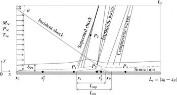
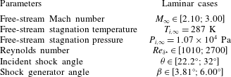
In the present study, an oblique shock wave/laminar-boundary-layer interaction is considered. The flow configuration is displayed in figure 1. To enable a comprehensive analysis of the unsteadiness of the structures developing in such a flow, a set of flow cases are run with parameters referenced in table 1. Hereafter, the coordinate system is the following:
 $x$
is oriented in the streamwise direction and
 $y$
is associated with the direction normal to the wall. Also
 $L_{sep}$
and
 $L_{int}$
the separation and interaction lengths, respectively.
The computational domain and a schematic representation of oblique shock wave/boundary-layer interaction.

Flow parameters for laminar OSWBLIs.

2.2. Governing equations
The two-dimensional compressible Navier–Stokes equations for a compressible perfect gas are considered. These equations govern the evolution of the system state
 $\boldsymbol{q}=[{\it\rho},{\it\rho}\boldsymbol{u},{\it\rho}E]^{\text{T}}$
in the conservative form, where
 ${\it\rho}$
,
 $\boldsymbol{u}$
and
 $E$
are the fluid density, the velocity vector and the total energy, respectively. Written in non-dimensional form, these equations are
 $$\begin{eqnarray}\displaystyle & \displaystyle \frac{\partial {\it\rho}}{\partial t}+\boldsymbol{{\rm\nabla}}\boldsymbol{\cdot }({\it\rho}\boldsymbol{u})=0, & \displaystyle\end{eqnarray}$$
 $$\begin{eqnarray}\displaystyle & \displaystyle \frac{\partial }{\partial t}({\it\rho}\boldsymbol{u})+\boldsymbol{{\rm\nabla}}\boldsymbol{\cdot }\left[{\it\rho}\boldsymbol{u}\otimes \boldsymbol{u}+p\boldsymbol{I}-\frac{1}{Re}{\bf\tau}\right]=\mathbf{0}, & \displaystyle\end{eqnarray}$$
 $$\begin{eqnarray}\displaystyle & \displaystyle \frac{\partial }{\partial t}({\it\rho}E)+\boldsymbol{{\rm\nabla}}\boldsymbol{\cdot }\left[({\it\rho}E+p)\boldsymbol{u}-\frac{1}{Re}{\bf\tau}\odot \boldsymbol{u}+\frac{{\it\kappa}}{({\it\gamma}-1)ReM_{\infty }^{2}}\boldsymbol{{\rm\nabla}}T\right]=0. & \displaystyle\end{eqnarray}$$
 $p$
and energy
 $E$
are related to the temperature through the equation of state for an ideal gas.
 $$\begin{eqnarray}p=\frac{1}{{\it\gamma}M_{\infty }^{2}}{\it\rho}T,\quad E=\frac{T}{{\it\gamma}({\it\gamma}-1)M_{\infty }^{2}}+\frac{1}{2}\boldsymbol{u}\boldsymbol{\cdot }\boldsymbol{u},\end{eqnarray}$$
 ${\bf\tau}$
is the viscous stress tensor and is written as
 $$\begin{eqnarray}{\bf\tau}={\it\mu}\left[\boldsymbol{{\rm\nabla}}\otimes \boldsymbol{u}+(\boldsymbol{{\rm\nabla}}\otimes \boldsymbol{u})^{\text{T}}-{\textstyle \frac{2}{3}}(\boldsymbol{{\rm\nabla}}\boldsymbol{\cdot }\boldsymbol{u})\boldsymbol{I}\right].\end{eqnarray}$$
The dynamics viscosity
 ${\it\mu}(T)$
is computed using Sutherland’s law, i.e.,
 $$\begin{eqnarray}{\it\mu}(T)=T^{3/2}\frac{1+T_{s}/T_{\infty }}{T+T_{s}/T_{\infty }},\end{eqnarray}$$
where
 $T_{s}=110.4~\text{K}$
. The coefficient of heat conductivity
 ${\it\kappa}(T)$
is given in terms of the Prandtl number
 ${\it\kappa}(T)={\it\mu}(T)/Pr$
. Here,
 $M_{\infty }$
is the free-stream Mach number at the inflow and
 $Re_{{\it\delta}^{\star }}$
is the Reynolds number based on the free-stream velocity downstream of the separated shock,
 $U_{e}$
, and the boundary layer displacement thickness at the theoretical position where the incident shock impinges the boundary-layer,
 ${\it\delta}^{\star }$
. The time scales are normalized with
 ${\it\delta}^{\star }/U_{e}$
and pressure with
 ${\it\rho}_{\infty }U_{e}^{2}$
. Finally, the specific heat capacity ratio is equal to
 ${\it\gamma}=1.4$
and the Prandtl number is taken as
 $Pr=0.72$
.
In the following, the system (2.1) can be recast in the formal conservative form:
 $$\begin{eqnarray}\frac{\partial \boldsymbol{q}}{\partial t}={\mathcal{R}}(\boldsymbol{q}),\end{eqnarray}$$
where
 ${\mathcal{R}}$
is the differential nonlinear Navier–Stokes operator.
2.3. Compressible global stability analysis
Linear stability analysis assumes the existence of an equilibrium solution to the system (2.5) referred to as the base flow and defined by
 ${\mathcal{R}}(\boldsymbol{q}_{b})=0$
. In the following, the base flow is assumed to be two-dimensional
 $\boldsymbol{q}_{b}(x,y)$
. Using the standard small-perturbation technique, the instantaneous flow is decomposed into a base flow and a small disturbance:
 $$\begin{eqnarray}\boldsymbol{q}(x,y,t)=\boldsymbol{q}_{b}(x,y)+{\it\varepsilon}\boldsymbol{q}^{\prime }(x,y,t),\quad {\it\varepsilon}\ll 1.\end{eqnarray}$$
The resulting equations are further simplified by considering that the perturbation is infinitesimal, i.e. the nonlinear fluctuating terms are neglected. Finally, the compressible Navier–Stokes equations are transformed into linear partial differential equations
 $$\begin{eqnarray}\frac{\partial \boldsymbol{q}^{\prime }}{\partial t}={\mathcal{J}}\boldsymbol{q}^{\prime },\end{eqnarray}$$
where the vector
 $\boldsymbol{q}^{\prime }=({\it\rho}^{\prime },{\it\rho}^{\prime }\boldsymbol{u}_{b}+{\it\rho}_{b}\boldsymbol{u}^{\prime },{\it\rho}^{\prime }E_{b}+{\it\rho}_{b}E^{\prime })^{\text{T}}$
represents the conservative variables for the perturbation and
 ${\mathcal{J}}=\partial {\mathcal{R}}/\partial \boldsymbol{q}|_{\boldsymbol{q}_{b}}$
is the Jacobian operator which corresponds to the linearization of the Navier–Stokes operator
 ${\mathcal{R}}$
around the base flow
 $\boldsymbol{q}_{b}$
.
 $$\begin{eqnarray}\frac{\partial {\it\rho}^{\prime }}{\partial t}+\boldsymbol{{\rm\nabla}}\boldsymbol{\cdot }({\it\rho}^{\prime }\boldsymbol{u}_{b}+{\it\rho}_{b}\boldsymbol{u}^{\prime })=0,\end{eqnarray}$$
 $$\begin{eqnarray}\frac{\partial }{\partial t}({\it\rho}^{\prime }\boldsymbol{u}_{b}+{\it\rho}_{b}\boldsymbol{u}^{\prime })+\boldsymbol{{\rm\nabla}}\boldsymbol{\cdot }\left({\it\rho}_{b}\boldsymbol{u}^{\prime }\otimes \boldsymbol{u}_{b}+{\it\rho}_{b}\boldsymbol{u}_{b}\otimes \boldsymbol{u}^{\prime }+{\it\rho}^{\prime }\boldsymbol{u}_{b}\otimes \boldsymbol{u}_{b}+p^{\prime }\boldsymbol{I}-\frac{1}{Re}{\bf\tau}^{\prime }\right)=\mathbf{0},\end{eqnarray}$$
 $$\begin{eqnarray}\displaystyle & & \displaystyle \frac{\partial }{\partial t}({\it\rho}^{\prime }E_{b}+{\it\rho}_{b}E^{\prime })+\boldsymbol{{\rm\nabla}}\boldsymbol{\cdot }\left[({\it\rho}_{b}E_{b}+p_{b})\boldsymbol{u}^{\prime }+({\it\rho}_{b}E^{\prime }+{\it\rho}^{\prime }E_{b}+p^{\prime })\boldsymbol{u}_{b}-\frac{1}{Re}{\bf\tau}^{\prime }\odot \boldsymbol{u}_{b}\right.\nonumber\\ \displaystyle & & \displaystyle \qquad \left.-\frac{1}{Re}{\bf\tau}_{b}\odot \boldsymbol{u}^{\prime }+\frac{{\it\kappa}^{\prime }}{({\it\gamma}-1)ReM_{\infty }^{2}}\boldsymbol{{\rm\nabla}}T_{b}+\frac{{\it\kappa}_{b}}{({\it\gamma}-1)ReM_{\infty }^{2}}\boldsymbol{{\rm\nabla}}T^{\prime }\right]=0,\end{eqnarray}$$
 $$\begin{eqnarray}{\bf\tau}^{\prime }={\it\mu}_{b}\left[(\boldsymbol{{\rm\nabla}}\otimes \boldsymbol{u}^{\prime }+\boldsymbol{{\rm\nabla}}\otimes \boldsymbol{u}^{\prime T})-{\textstyle \frac{2}{3}}(\boldsymbol{{\rm\nabla}}\boldsymbol{\cdot }\boldsymbol{u}^{\prime })\boldsymbol{I}\right]+{\it\mu}^{\prime }\left[(\boldsymbol{{\rm\nabla}}\otimes \boldsymbol{u}_{b}+\boldsymbol{{\rm\nabla}}\otimes \boldsymbol{u}_{b}^{\text{T}})-{\textstyle \frac{2}{3}}(\boldsymbol{{\rm\nabla}}\boldsymbol{\cdot }\boldsymbol{u}_{b})\boldsymbol{I}\right].\end{eqnarray}$$
The perturbed pressure, total energy, dynamic viscosity and heat conductivity coefficient are written
 $$\begin{eqnarray}p^{\prime }=\frac{1}{{\it\gamma}M_{\infty }^{2}}({\it\rho}_{b}T^{\prime }+{\it\rho}^{\prime }T_{b}),\quad E^{\prime }=\frac{T^{\prime }}{{\it\gamma}({\it\gamma}-1)M_{\infty }^{2}}+\boldsymbol{u}_{b}\boldsymbol{\cdot }\boldsymbol{u}^{\prime },\quad {\it\mu}^{\prime }=\frac{\partial {\it\mu}_{b}}{\partial T_{b}}T^{\prime },\quad {\it\lambda}^{\prime }=\frac{{\it\mu}^{\prime }}{Pr}.\end{eqnarray}$$
3. Numerical strategy
3.1. Navier–Stokes solver and boundary conditions
All numerical simulations in this paper were run with an in-house CFD solver named Phoenix, both to compute the base flow and to solve the linearized and the full Navier–Stokes equations. The numerical method implemented in our solver is based on the finite-volume approach and on a cell-centred discretization. The code solves the compressible Navier–Stokes equations on multi-block structured grids and these equations are discretized in space using an upwind scheme. Roe’s flux difference splitting scheme (Roe Reference Roe1981) is employed to obtain advective fluxes at the cell interface for all N–S equations. The MUSCL approach extends the spatial accuracy to third order. All viscous terms are centrally differentiated. For unsteady computations, the dual time stepping method, proposed by Jameson (Reference Jameson1991), was used to tackle the lack of numerical efficiency of the global time stepping approach. The derivative with respect to the physical time is discretized by a second-order formula. The use of an implicit scheme with respect to the dual time provides fast convergence to the time-accurate solution. Between each time step, the solution is advanced in a dual time and acceleration strategies developed for steady problems can be used to speed up the convergence in fictitious time. The implicit time-integration procedure leads to a system which can be solved directly or iteratively. The direct inversion can be memory intensive and computationally expensive. Therefore, an implicit relaxation procedure is preferred and the point Jacobi relaxation algorithm was chosen. The initialization of the derivative with respect to the physical time was performed with a first-order formula.
The boundary conditions applied to the computational domain are no-slip velocity, adiabatic temperature and pressure extrapolation at the wall. The steady two-dimensional Navier–Stokes solution is imposed at the inflow. To minimize the reflection of waves into the domain at the outflow and at the upper boundary, a characteristic method is used for the conservative variables. The oblique shock is imposed by the Rankine–Hugoniot jump relations at the top boundary.
3.2. Linearization of discrete Navier–Stokes equations
Equations (2.8) are discretized with the same type of scheme as the nonlinear N–S equations (2.1). However, the spatial schemes as well as boundary conditions have to be adapted to the new set of equations (2.8). To achieve such a task, the different schemes and boundary conditions are built by considering the flux function associated with the linearized equations (2.8). The Roe scheme is adopted in this study. As suggested by Crouch, Garbaruk & Magidov (Reference Crouch, Garbaruk and Magidov2007), the Roe scheme adapted for the linearized compressible N–S variables is based on the Jacobian matrix of the new flux function associated with the linearized equations, as discussed above. The latter matrix being only a function of the base flow, there is no need for a Roe average. In addition, the boundary conditions are also only driven by the base flow, yielding similar modifications of our CFD solver. Finally the semi-discrete system can be written as
 $$\begin{eqnarray}\frac{\text{d}\boldsymbol{q}^{\prime }}{\text{d}t}=\unicode[STIX]{x1D645}\boldsymbol{q}^{\prime },\end{eqnarray}$$
where
 $\unicode[STIX]{x1D645}$
is
 $(n\times n)$
Jacobian matrix and
 $n=\text{dim}(\boldsymbol{q}^{\prime })\times n_{x}\times n_{y}$
.
3.3. Stability algorithm
To determine the eigenmodes of discrete linearized Navier–Stokes equations (3.1) the solution is sought under the form of a normal mode
 $\boldsymbol{q}^{\prime }(\boldsymbol{x},t)=\widehat{\boldsymbol{q}}(\boldsymbol{x})\exp ({\it\lambda}t)$
, the problem (3.1) becomes an eigenproblem
 $\unicode[STIX]{x1D645}\widehat{\boldsymbol{q}}={\it\lambda}\widehat{\boldsymbol{q}}$
where
 ${\it\lambda}={\it\sigma}+\text{i}{\it\omega}$
is the eigenvalue and
 $\widehat{\boldsymbol{q}}$
is the eigenvector. The sign of the leading eigenvalue’s real part
 ${\it\sigma}$
then determines whether the fixed point
 $\boldsymbol{q}_{b}$
is linearly stable or unstable, whereas its imaginary part
 ${\it\omega}$
characterizes the stationary or oscillatory nature of the associated eigenvector. To solve this eigenproblem, two types of methods can be used: (i) methods where the Jacobian matrix is explicitly formed or (ii) methods wherein the matrix is not directly and fully calculated, these methods are known as matrix-free methods. In the present configuration, the size of our problem (
 $\unicode[STIX]{x1D645}$
would be approximately a
 $10^{5}\times 10^{5}$
matrix) is not limiting and both methods are possible. The matrix-free method is selected where snapshots of the solution of (3.1) are used to approximate the Jacobian matrix. In the compressible regime, this method has a number of advantages because it is written in a fully-discrete formalism allowing to better take into account the complex boundary conditions such as the presence or the emission of acoustic waves while maintaining an accurate description of the hydrodynamic instability. Using a snapshot method based on the discrete equation (3.1), we solve the following eigenvalue problem
 $\unicode[STIX]{x1D648}({\rm\Delta}t_{s})\boldsymbol{q}^{\prime }=\widehat{{\it\lambda}}\boldsymbol{q}^{\prime }$
, where
 $\unicode[STIX]{x1D648}({\rm\Delta}t_{s})=\exp (\unicode[STIX]{x1D645}{\rm\Delta}t_{s})$
is the exponential propagator of the system (3.1). It appears at first sight that this so-called time stepper approach (Edwards et al.
Reference Edwards, Tuckerman, Friesner and Sorensen1994; Bagheri et al.
Reference Bagheri, Akervik, Brandt and Henningson2009) does not really simplify the initial problem of memory footprint. Indeed, not only is
 $\exp (\unicode[STIX]{x1D645}{\rm\Delta}t_{s})$
a matrix of very large dimensions, but it is well known that computing a matrix exponential can be quite a challenging computational task. The most interesting feature of such a time-stepper approach however is that, though
 $\exp (\unicode[STIX]{x1D645}{\rm\Delta}t_{s})$
is as computationally expensive to construct explicitly as the Jacobian
 $\unicode[STIX]{x1D645}$
, the action of this exponential propagator on a vector
 $\boldsymbol{q}_{0}^{\prime }$
can easily be approximated by simply time marching the linearized Navier–Stokes equations (3.1) with
 $\boldsymbol{q}_{0}^{\prime }$
as the initial condition. The eigenmodes of
 $\unicode[STIX]{x1D648}$
are the same as those of the matrix
 $\unicode[STIX]{x1D645}$
if
 ${\rm\Delta}t_{s}$
is chosen in accordance with the Nyquist criterion. The dataset length
 $N_{s}{\rm\Delta}t_{s}$
is sufficient to capture the slowest frequency of the system by a factor 20 (see table 2). The iterative technique is based on the orthogonal projection of the large matrix
 $\unicode[STIX]{x1D648}$
onto a lower-dimensional Krylov subspace which is spanned by snapshots taken from the flow field
 $\boldsymbol{q}^{\prime }$
separated by a constant time interval
 ${\rm\Delta}t_{s}$
. The resulting system is a significantly smaller system and can be solved using classical direct or iterative methods:
 $$\begin{eqnarray}\boldsymbol{K}_{m}(\unicode[STIX]{x1D648},\boldsymbol{q}_{0}^{\prime })=\text{span}[\boldsymbol{q}_{0}^{\prime },\unicode[STIX]{x1D648}\boldsymbol{q}_{0}^{\prime },\unicode[STIX]{x1D648}^{2}\boldsymbol{q}_{0}^{\prime },\ldots ,\unicode[STIX]{x1D648}^{m-1}\boldsymbol{q}_{0}^{\prime }]=\text{span}[\boldsymbol{q}_{0}^{\prime },\boldsymbol{q}_{1}^{\prime },\boldsymbol{q}_{2}^{\prime },\ldots ,\boldsymbol{q}_{m-1}^{\prime }].\end{eqnarray}$$
To increase the conditioning of the Krylov basis, a Gram–Schmidt orthogonalisation process is used. The exponential propagator matrix
 $\exp (\unicode[STIX]{x1D645}{\rm\Delta}t_{s})$
is then projected on this unitary basis
 $\boldsymbol{U}$
:
 $$\begin{eqnarray}\unicode[STIX]{x1D648}\boldsymbol{U}_{k}=\boldsymbol{U}_{k}\unicode[STIX]{x1D643}_{k}+\boldsymbol{r}_{k}\boldsymbol{e}_{k}^{\text{T}},\end{eqnarray}$$
where
 $\boldsymbol{U}_{k}$
is an orthonormal set of vectors,
 $\unicode[STIX]{x1D643}_{k}$
a
 $k\times k$
upper Hessenberg matrix and
 $\boldsymbol{r}_{k}\boldsymbol{e}_{k}^{\text{T}}$
is the residual vector indicating how far from an invariant subspace of
 $\unicode[STIX]{x1D648}$
is
 $\boldsymbol{U}_{k}$
. Because of its relatively small dimension, the eigenpairs (
 $\widehat{{\it\lambda}}_{H},\boldsymbol{X}$
) of the Hessenberg matrix can be directly computed which are a good approximation to those of
 $\unicode[STIX]{x1D648}$
. Since this Hessenberg matrix is a low-dimensional approximation of the exponential propagator
 $\unicode[STIX]{x1D648}=\exp (\unicode[STIX]{x1D645}{\rm\Delta}t_{s})$
, these Ritz pairs are linked to the eigenpairs of the Jacobian matrix
 $\unicode[STIX]{x1D645}$
by:
 $$\begin{eqnarray}\left.\begin{array}{@{}c@{}}{\it\lambda}\simeq \displaystyle \frac{\log (\widehat{{\it\lambda}}_{H})}{{\rm\Delta}t_{s}},\\ \widehat{\boldsymbol{q}}\simeq \boldsymbol{U}_{k}\boldsymbol{X}.\end{array}\right\}\end{eqnarray}$$
The easiest way to solve the eigenvalue problem for a matrix-free method is (i) to force the system (3.1) by an impulse-shaped parietal forcing; (ii) to generate the set of snapshots; and (iii) to solve the eigenproblem by an Arnoldi method. Although this method is used to calculate with good accuracy the unstable modes, the stable part of the spectrum is more difficult to obtain. When the flow is globally stable (selective noise amplifier behaviour) this problem becomes critical. The origin of the problem is two-fold. For the open flows, the linearized evolution operator is often highly non-normal, the eigenvalues are then highly sensitive to perturbations (Trefethen & Embree Reference Trefethen and Embree2005; Schmid Reference Schmid2007). In addition, a snapshot method, which is similar to a signal processing method, is ill conditioned for temporally stable flows because over time the modes fade, making it more difficult to extract their frequency content. To solve this problem, the computation of the matrix
 $\unicode[STIX]{x1D643}$
from numerical simulations is accomplished by an in-house Arnoldi method (Arnoldi Reference Arnoldi1951; Lehoucq, Sorensen & Yang Reference Lehoucq, Sorensen and Yang1997; Barkley, Blackburn & Sherwin Reference Barkley, Blackburn and Sherwin2008) directly integrated into the temporal loop of our CFD solver (see Loiseau et al.
Reference Loiseau, Robinet, Cherubini and Leriche2014).
4. Laminar OSWBLI cases
4.1. Base flows
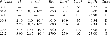
Seven flow cases will be considered hereafter, referenced A–G in table 3. For all flow cases, a preliminary laminar boundary-layer flow computation without an impinging shock is carried out. Then we denote by
 ${\it\delta}^{\star }$
the displacement thickness at the position of impact of the incident shock. For flow case A, the flow conditions are matched to the experimental and numerical investigation of Degrez et al. (Reference Degrez, Boccadoro and Wendt1987). The free-stream Mach number is
 $M_{\infty }=2.15$
and the angle of the incident shock measured clockwise from the horizontal axis is
 ${\it\theta}=30.8^{\circ }$
(corresponding to a flow deflection angle of
 $3.81^{\circ }$
). The Reynolds number based on
 ${\it\delta}^{\star }$
is fixed to
 $Re_{{\it\delta}^{\star }}=1050$
. The computational domain
 ${\mathcal{D}}$
has dimensions
 $[x_{0}/{\it\delta}^{\star };x_{n}/{\it\delta}^{\star }]\times [y_{0}/{\it\delta}^{\star };y_{n}/{\it\delta}^{\star }]=[0;400]\times [0;80]$
in the streamwise and wall-normal directions, respectively. The total number of points that are clustered in the normal-to-wall direction, as well as in the interaction region, is
 $(N_{x}\times N_{y})=(560\times 100)$
. Numerical validations (not shown here for the sake of conciseness) have proven that this guarantees grid independency. The dual time step is switched off and the CFL (Courant–Friedrichs–Lewy) number is held to 10.
Numerical set-up for the different stability computations.
 ${\rm\Delta}t$
is the time stepping used in linearized Navier–Stokes solver,
 ${\rm\Delta}t_{s}$
is the time between two consecutive snapshots,
 $N_{s}$
is the number of snapshots,
 ${\it\varepsilon}_{ev}$
is the minimal eigenvalues convergence.

Flow parameters for the OSWBLI.

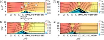
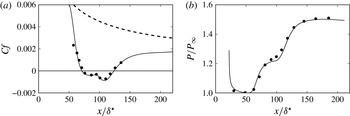
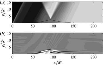
After having reached a steady state for the laminar boundary-layer flow, the incident shock is introduced at the inflow condition through the Rankine–Hugoniot relations. The latter shock impinges the boundary-layer, which creates a separated flow. It thus leads to compression waves behind the bubble which coalesce to form the reflected or separated shock. The converged base flow is shown in figure 2(a) in terms of streamwise velocity fields and streamlines. Comparisons with both experimental and numerical results given by Degrez et al. (Reference Degrez, Boccadoro and Wendt1987) are displayed in figure 3. The latter figure shows that our simulation is in good agreement with the mean-flow characteristics reported by Degrez et al. (Reference Degrez, Boccadoro and Wendt1987), both in terms of friction coefficient and wall pressure measurements.
Streamlines and streamwise velocity component of the computed steady base flow for different values for Reynolds and Mach numbers and incident angles. The incident shock (1), the reflected shock (2), the expansion fan (3) and compression waves (4) are also represented. (a)
 $Re_{{\it\delta}^{\star }}=1050$
,
 $M_{\infty }=2.15$
and
 ${\it\theta}=30.8^{\circ }$
, (b)
 $Re_{{\it\delta}^{\star }}=1050$
,
 $M_{\infty }=2.15$
and
 ${\it\theta}=32^{\circ }$
, (c)
 $Re_{{\it\delta}^{\star }}=1090$
,
 $M_{\infty }=2.20$
and
 ${\it\theta}=30.8^{\circ }$
, (d)
 $Re_{{\it\delta}^{\star }}=1950$
,
 $M_{\infty }=2.15$
and
 ${\it\theta}=30.8^{\circ }$
.

Flow case A. (a) Friction coefficient and (b) wall pressure distribution normalized by
 $P_{\infty }$
shown as a function of the streamwise position scaled by
 ${\it\delta}^{\star }$
. Full line: our computation. Full circle, the results given by Degrez et al. (Reference Degrez, Boccadoro and Wendt1987). (a) The dashed-line is associated with the friction coefficient of the laminar boundary layer without the impinging incident shock.

In order to investigate the influence of various physical parameters (bubble shapes,
 $M_{\infty }$
and
 $Re_{{\it\delta}^{\star }}$
) on stability properties, equilibrium states associated with B–G are also computed (see figure 2
b–d).
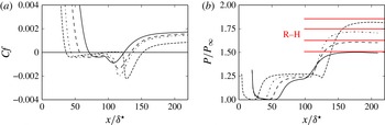
Figure 4(a,b) show the distribution of skin-friction coefficients and dimensionless pressure, respectively, as a function of the streamwise position
 $x$
for
 ${\it\theta}$
varying from
 $30.8^{\circ }$
to
 $32.5^{\circ }$
when the Reynolds number and the Mach number are fixed to 1050 and 2.15, respectively. It is observed that when the incident angle increases, the interaction zone increases almost linearly. Figure 4(a) also shows that for an angle close to
 $32.5^{\circ }$
(computed for the same flow conditions in terms of Mach and Reynolds numbers), there is a critical point (around
 $x/{\it\delta}^{\star }\simeq 99.2$
) where the skin-friction coefficient becomes positive. In an incompressible regime, Theofilis et al. (Reference Theofilis, Hein and Dallmann2000) and Rodriguez & Theofilis (Reference Rodriguez and Theofilis2010) have shown that the latter behaviour is associated with a bifurcation of the flow towards a three-dimensional state. This behaviour has also been observed for supersonic separated flows by Boin et al. (Reference Boin, Robinet, Corre and Deniau2006) and Robinet (Reference Robinet2007). Hence, the figure 4(a) suggests that
 ${\it\theta}=32.5^{\circ }$
is a relevant upper limit when considering a two-dimensional equilibrium state. Figure 4(b) shows that the pressure ratio reaches the value provided by the Rankine–Hugoniot relationship downstream of the reflected shock for the different incident angles
 ${\it\theta}$
studied. Hereafter, the stability analysis will be limited to the incident angles
 ${\it\theta}\leqslant 32^{\circ }$
. Similar behaviour is observed when the Reynolds number and/or Mach number are increased.
 $M_{\infty }=2.15$
,
 $Re_{{\it\delta}^{\star }}=1050$
. Distributions of (a) skin-friction coefficient and (b) dimensionless pressure with the streamwise position. The values provided by the Rankine–Hugoniot relationship are also provided as horizontal full lines labelled R–H. Full line:
 ${\it\theta}=30.8^{\circ }$
, long dashed line:
 ${\it\theta}=31.4^{\circ }$
, dash-dot line:
 ${\it\theta}=32^{\circ }$
and dashed line:
 ${\it\theta}=32.5^{\circ }$
.

4.2. Global mode analysis and linear dynamics
4.2.1. Linear impulse response
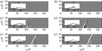
According to Huerre & Monkewitz (Reference Huerre and Monkewitz1990), the onset of unsteadiness in open flows may be classified into two categories. In particular, the flow behaves either as a noise amplifier or an oscillator. To emphasize the specificity of the OSWBLI, we first consider its response to a localized impulse placed close to the inlet. The space and time behaviour of the resulting wavepacket is illustrated in figures 5–7.
Case A: linear dynamics of the wavepacket resulting from an impulsive perturbation localized at (a)
 $t=64~{\it\delta}^{\star }/U_{e}$
, (b)
 $t=91~{\it\delta}^{\star }/U_{e}$
, (c)
 $t=119~{\it\delta}^{\star }/U_{e}$
, (d)
 $t=146~{\it\delta}^{\star }/U_{e}$
, (e)
 $t=174~{\it\delta}^{\star }/U_{e}$
and ( f)
 $t=202~{\it\delta}^{\star }/U_{e}$
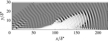
. The shaded contours represent the pressure fluctuations. The line contours represent the spanwise vorticity component of the velocity fluctuation fields.

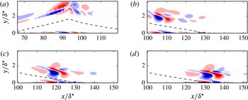
Case A: the spanwise vorticity component of the velocity fluctuation fields associated with the linear dynamics of the wavepacket shown in figure 5 represented for (a)
 $t=91~{\it\delta}^{\star }/U_{e}$
, (b)
 $t=119~{\it\delta}^{\star }/U_{e}$
, (c)
 $t=146~{\it\delta}^{\star }/U_{e}$
, (d)
 $t=174~{\it\delta}^{\star }/U_{e}$
. The separation line is depicted by the dashed lines. Negative values in blue; positive values in red.

Case A: Space–time diagram for the linear dynamics resulting from an impulsive perturbation localized at
 $x/{\it\delta}^{\star }=20$
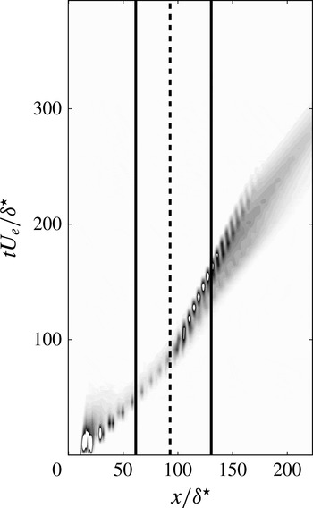
. The vertical axis is the dimensionless time. The horizontal axis is the dimensionless streamwise position. The shaded contours represent the kinetic energy associated with the velocity fluctuation fields. The bold vertical lines are associated with the separation point and point of reattachment.

 $M_{\infty }=2.15$
,
 ${\it\theta}=30.8^{\circ }$
and
 $Re_{{\it\delta}^{\star }}=1050$
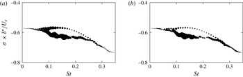
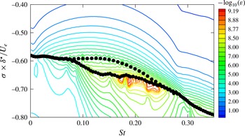
(Case A): global spectrum showing the temporal amplification rate
 ${\it\sigma}{\it\delta}^{\star }/U_{e}$
versus the Strouhal number
 $St=({\it\omega}{\it\delta}^{\star }/U_{e})/2{\rm\pi}$
. Where
 ${\it\delta}^{\star }$
and
 $U_{e}$
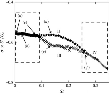
are the displacement thickness taken at the impact of the oblique shock and the external velocity downstream of separated shock. Each region shows the least stable eigenvalues belonging to region I: supersonic Kelvin–Helmholtz modes (circles), region II: subsonic Kelvin–Helmholtz modes (stars), region III: boundary-layer modes (crosses) and region IV: acoustic modes (
 $+$
).

Figures 5 and 6 show multiple snapshots of the wavepacket at different times. In these figures, the linear response of the flow exhibits a transient temporal growth when evolving downstream along the flat plate, characteristic of noise amplifier dynamics. In figure 6, the spanwise vorticity component of the velocity fluctuation field is shown in the vicinity of the separation line for different times. In particular, the wavepacket takes the form of vortices that evolve into a single row of alternating sign structures along the separation line. These vortices are reminiscent of ones that develop in a mixing layer under the action of a Kelvin–Helmholtz convective instability mechanism. In addition, while the wavepackets grow along the shear layer, we observe the emission of acoustic waves radiated into the expansion fan when the latter crosses the impact point of the incident shock. The wavepacket dynamics is also illustrated through the space–time diagram shown in figure 7 where the distribution of the integrated kinetic energy along the wall normal direction
 $E(x,t)=\int _{y=0}^{L_{y}}{\it\rho}(u^{2}+v^{2}+w^{2})\,\text{d}y$
(where
 $L_{y}$
is associated with the upper limit along the direction normal to the wall) is represented as a function of the streamwise position and time. Figure 7 shows that the upstream front velocity of the wavepacket decreases slowly after the impact point of the incident shock and accelerates again when it reaches the attached zone. Then, it leaves smoothly the computational domain and the flow relaxes to its equilibrium state. In addition, figure 7 clearly illustrates the non-parallel and dispersive effects of the wavepacket space–time dynamics. Cossu & Chomaz (Reference Cossu and Chomaz1997) have demonstrated that the convective nature of the wavepacket can be interpreted as a consequence of the streamwise non-normality of global modes (see Chomaz (Reference Chomaz2005) for a recent review). In this context, the noise amplifier behaviour can be captured by a suitable superposition of global modes that lead to transient energy growth. To illustrate the observed wavepacket behaviour, the global modes, temporal and spatial scales, are investigated in the next section which in turn will allow for an interpretation of both numerical and experimental observations of shock wave/boundary-layer interaction dynamics.
4.2.2. Features of the global spectrum
The algorithm outlined in § 3.3 is applied to linear simulations of shock wave/boundary-layer interaction referenced in table 3. Details on the numerical parameters are given in table 2. Hereafter, the dimensionless frequency based on
 ${\it\delta}^{\star }$
and
 $U_{e}$
is given by the Strouhal number
 $St=({\it\omega}{\it\delta}^{\star }/U_{e})/2{\rm\pi}$
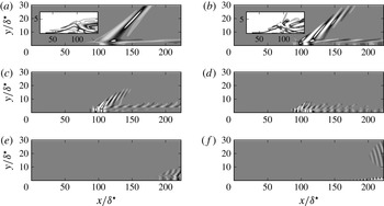
. Figure 8 shows the global spectrum for case A. Additional computations were carried out for different grids (see § A.1) showing a good approximation of the eigenspectrum for the grid used in this section. The growth rate of each eigenvalue is negative. This means that all of the modes are temporally damped consistent with the noise amplifier dynamics observed in the previous section. In figure 8, we observe that the global modes are grouped in different regions. Figure 9(a,b) shows the real part of the perturbation pressure associated with modes labelled (a) and (b) in figure 8. It clearly shows that vortical structures are mainly localized in the separated area and emit a beam of acoustic radiation into the far field. From its spanwise vorticity component, we observe that the latter type of modes display typical features of Kelvin–Helmholtz instabilities developing along the shear layer. In addition, figure 9(a,b) shows that while the structures are tilted against the shear behind the impact of the incident shock, they are reoriented along the shear direction afterwards.
Case A: representatives global modes of regions I (a–c), II (d), III (e) and IV ( f), marked with arrows in figure 8. The real part of the normalized perturbation pressure by the integrated kinetic energy is shown. Contours levels range from
 $-0.5$
to 0.5 in steps of 0.1. In (a), the real part of the spanwise vorticity component in the separated zone is visualized. Contours levels range from
 $-5$
to 5 with a step of 1.

The shear layer generated by the separation is composed of an upper and a lower stream, referenced hereafter by
 $\bullet _{1}$
and
 $\bullet _{2}$
, respectively. The relative phase velocities are defined as
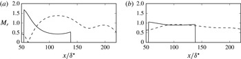
 $$\begin{eqnarray}M_{r,i}=\frac{|{\it\omega}/{\it\alpha}_{r}-U_{i}|}{a_{i}},\end{eqnarray}$$
with
 $U_{i}$
,
 $a_{i}$
(
 $i=1,2$
) the streamwise velocity component and the speed of sound associated with the base flow, respectively. The wavenumber of the mode in a curvilinear coordinates (
 $s$
) system attached to the shear layer is
 ${\it\alpha}_{r}$
, its circular frequency is
 ${\it\omega}$
. In particular, as underlined by Cheung & Lele (Reference Cheung and Lele2009), the instability waves are classified as subsonic or supersonic if
 $M_{r}<1$
or
 $M_{r}>1$
, respectively. In a global modes framework, as recently shown by Song et al. (Reference Song, Alizard, Robinet and Gloerfelt2013), the wavenumber can be extracted from the eigenmode by
 $$\begin{eqnarray}{\it\phi}=\tan ^{-1}\left(\frac{\hat{v}_{i}}{\hat{v}_{r}}\right),\quad {\it\alpha}_{r}=\frac{\text{d}{\it\phi}}{\text{d}s}.\end{eqnarray}$$
In figure 10(a,b), we show the relative phase speed of modes labelled (b) and (c) in figure 9. While the modes have a subsonic phase speed in the lower stream, they exhibit a supersonic phase speed in the upper stream behind the incident shock. Hence, the instability waves propagate supersonically with respect to the exterior fluid in the upper stream and create Mach wave radiation (Tam & Burton Reference Tam and Burton1984) in the localized region close to the expansion fan. Hence, the modes belonging to region I are referred to as supersonic Kelvin–Helmholtz modes.


Besides supersonic Kelvin–Helmholtz modes, the flow also contains modes with a large contribution of the pressure fluctuations in the free stream (region IV) shown in figure 9( f). The latter modes travel downstream and emit an acoustic radiation in the free stream with a downstream directivity. In a global stability framework, as recently noted by Nichols & Lele (Reference Nichols and Lele2011), to visualize the neutrally propagating part of the global acoustic mode travelling downstream, we have to post-multiply the pressure component by
 $\exp (-k_{i}(x-x_{s}))$
. The transformation
 $k_{i}=-{\it\sigma}/(U_{\infty }+c_{0})$
is used to convert the temporal growth rate
 ${\it\sigma}$
to the spatial one
 $-k_{i}$
where
 $c_{0}$
and
 $U_{\infty }$
stand for the speed of sound and the streamwise velocity in the free stream, respectively. In figure 11, we show the neutrally propagating part of the global mode labelled ( f) in figure 9. It exhibits a beam of acoustic radiation that is directive with a shallow emission angle from a source localized close to the impact of the incident shock. The latter modes are reminiscent of superdirective global modes observed in a cold supersonic jet by Nichols & Lele (Reference Nichols and Lele2011). Different computations were carried out for different domain sizes in the streamwise direction. The results appear independent of the domain.
The neutrally propagating part of the pressure component associated with the global mode shown in figure 9( f).

In the intermediate frequencies (regions II and III), we observe in figure 8 that the spectrum exhibits two distinct kinds of modes. While the least temporally damped modes are associated with Kelvin–Helmholtz modes that travel with a subsonic relative phase speed along the shear layer, the second one consists of boundary-layer modes as shown in figure 9(e). Hence, the modes associated with regions II and III are referred to as subsonic Kelvin–Helmholtz modes and boundary-layer modes, respectively.
The global spectrum shows that a wide range of physical processes exists, associated with different families of modes that exhibit a distinct characteristic frequency. In addition, these characteristic frequencies are seen to be independent of the computational domain size. It is thus clear that, while modes of regions I, II and III may play an important role on the space–time behaviour of the wavepacket associated with a linear impulse (discussed in the previous section), radiating modes of region IV do not seem to be involved in such dynamics.
Finally, one may also remark that the spectrum obtained in the laminar regime differs from those given by Pirozzoli et al. (Reference Pirozzoli, Larsson, Nichols, Bernardini, Morgan and Lele2010) and Sartor et al. (Reference Sartor, Mettot, Bur and Sipp2015) associated with supersonic and transonic turbulent shock wave/boundary-layer interactions, respectively. For instance, the least damped mode obtained by Pirozzoli et al. (Reference Pirozzoli, Larsson, Nichols, Bernardini, Morgan and Lele2010) is non-oscillatory and concentrated in the recirculation zone. The latter authors suggest that this mode plays a predominant role in the low-frequency dynamics of this flow. However, such a mode is not observed in the present computation. Furthermore, the least damped global modes associated with transonic channel flow over a bump computed recently by Sartor et al. (Reference Sartor, Mettot, Bur and Sipp2015) are acoustic resonance modes and shock-wave low-frequency modes. Sartor et al. (Reference Sartor, Mettot, Bur and Sipp2015) conclude that the major part of the stable modes are probably not linked to the unsteady dynamics observed in turbulent SWBLI. In our case, from observations of the impulse response in the linear regime, it seems clear that the space–time dynamics of the laminar OSWBLI is closely associated with global modes.
4.2.3. Scaling analysis
As the above discussion suggests, the linear dynamics of a OSWBLI involves a wide variety of global modes with various frequencies and spatial scales. Of particular interest is the dependence of the characteristic frequencies on the representative spatial scales. For this purpose, we will attempt to define a suitable scaling for both supersonic and subsonic Kelvin–Helmholtz modes and boundary-layer modes. This will be done by considering the interaction length (
 $L_{int}$
) and the displacement thickness at the impact (
 ${\it\delta}^{\star }$
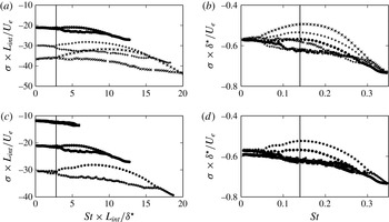
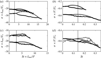
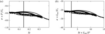
). Trying to unravel the Reynolds and Mach number effects, we show in figure 12 global spectra associated with flow cases A–E where both the Reynolds number and the Mach number are kept nearly constant. Hence, in the latter five cases, we mainly focus on the influence of the bubble shape by means of minor variations of the Mach number (flow cases D and E) or the angle of the incident shock (flow cases B and C) around the reference case A. In figure 13, global spectra for flow cases F and G associated with different Reynolds and Mach numbers are displayed. In figures 12 and 13 the frequencies and the temporal amplification rates are scaled either by
 $L_{int}$
or
 ${\it\delta}^{\star }$
. Figure 12 gives some evidence that the driving mechanism for the unsteadiness associated with supersonic Kelvin–Helmholtz modes is based on the characteristic length
 $L_{int}$
. In particular, the separation between regions I and II/III occurs for
 $St\times L_{int}/{\it\delta}^{\star }\approx 2.8$
for flow cases A–E.
Global spectra showing the temporal amplification rate versus the Strouhal number. (a,c) The frequencies and the growth rate are scaled by
 $L_{int}$
and
 $U_{e}$
. (b,d) The frequencies and the growth rate are scaled by
 ${\it\delta}^{\star }$
and
 $U_{e}$
. ●,
 $+$
,
 $\times$
, ▪ and
 $\star$
are associated with flow cases A–E, respectively. The vertical lines correspond to
 $St\times L_{int}/{\it\delta}^{\star }\approx 2.8$
(a,c) and
 $St\approx 0.145$
(b,d).

Global spectra showing the temporal amplification rate versus the Strouhal number. (a,c) The frequencies and the growth rate are scaled by
 $L_{int}$
and
 $U_{e}$
. (b,d) The frequencies and the growth rate are scaled by
 ${\it\delta}^{\star }$
and
 $U_{e}$
. ●, ▸ and ▴ are associated with flow cases A, F and G, respectively. The vertical lines correspond to
 $St\times L_{int}/{\it\delta}^{\star }\approx 2.8$
(a,c) and
 $St\approx 0.145$
(b,d).

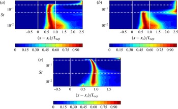
Distribution of integrated kinetic energy along the wall normal direction as a function of the streamwise position for frequencies associated with global modes for (a,b): flow case A and (c) flow case C. (a) Regions I, II, IV are considered. (b) Regions I, III and IV are considered. The horizontal lines denotes the position associated with the separation between modes of regions I and II/III and separation between modes of regions II/III and region IV. Vertical lines denote the separation and the reattachment points.

In contrast to the latter modes, both the subsonic Kelvin–Helmholtz modes and boundary-layer modes appear to scale with the local scale
 ${\it\delta}^{\star }$
for a given couple of Reynolds and Mach numbers. In particular, for cases A–E, the least damped mode associated with region II oscillates with a frequency
 $St\approx 0.145$
. In addition, as expected, a slight increase in
 $M_{\infty }$
and/or
 ${\it\theta}$
leads to an increase in the temporal amplification rates of mode II. Furthermore, when considering flow cases A and F, we may observe that a large increase of the Reynolds number leads to decrease the dominant frequencies associated with region II, when the latter are made dimensionless by
 ${\it\delta}^{\star }$
(see figure 13
b). In contrast, the separation between subsonic and supersonic Kelvin–Helmholtz modes is not affected (see figure 13
a). When focusing on the Mach number effect, figure 13(d) shows that an increase in Mach number leads to higher frequencies for the subsonic Kelvin–Helmholtz waves. In addition, the modes belonging to region I are displaced further to the lower frequency range when scaled by
 $U_{e}$
and
 $L_{int}$
as shown in figure 13(c). The latter remark seems to show that the gap between the lowest frequencies and those associated with subsonic Kelvin–Helmholtz modes widens with an increase of the Mach number. However, it is clear that making definite statements regarding Reynolds and Mach number effects is a hard task, mainly due to the difficulty of changing the two parameters separately. To give further insight into the observed scaling, we provide in figure 14 the distribution of the integrated kinetic energy along the wall-normal direction for each global mode as a function of the streamwise coordinate for flow cases A and C. It is interesting to note that the energy associated with the region I frequencies (i.e. supersonic Kelvin–Helmholtz modes) are mainly localized in the separation zone; whereas frequencies for region II (i.e. subsonic Kelvin–Helmholtz modes) are strongly concentrated near the reattachment point. This behaviour tends to be more pronounced with an increase of the separation zone as observed in figure 14(c). It thus provides more evidence that frequencies for region I are driven by a scale proportional to the separation or interaction length whereas frequencies for region II are governed by a local scale
 ${\it\delta}^{\star }$
. Finally, one may also remark that figure 14(a,b) clearly show the spatial separation between subsonic Kelvin–Helmholtz modes and boundary-layer modes. In particular, the latter modes are spatially amplified in the attached region downstream of the bubble.
4.3. Linear regime: noise amplifier dynamics and receptivity
In the previous sections, we have shown that OSWBLI is globally stable for a wide range of angles of the incident shock, and of Reynolds and Mach numbers. The flow behaviour will thus depend on the receptivity (i.e. associated with both the level and the shape of the external noise; and the way it affects the flow) and a frequency-selective noise amplification of the external perturbation due to non-orthogonal interactions between the modes (see Schmid (Reference Schmid2007) for a review).
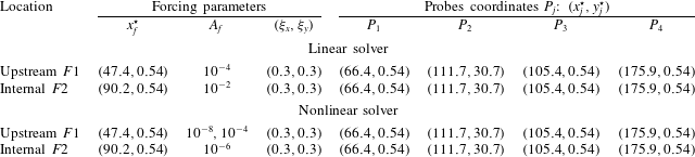
To give insight into the selection frequency process of such a flow, we investigate the linear flow response to a white noise excitation (i.e. the linear version of the CFD code is used). For this purpose, a spatially localized forcing near the wall is chosen as actuator. In particular, the latter has a Gaussian envelope:
 $$\begin{eqnarray}v_{f}^{\prime }(x^{\star },y^{\star })=A_{f}\exp \left[-\!\left(\frac{x^{\star }-x_{f}^{\star }}{{\it\xi}_{x}}\right)^{2}-\left(\frac{y^{\star }-y_{f}^{\star }}{{\it\xi}_{y}}\right)^{2}\right]\cdot W_{v}(t),\end{eqnarray}$$
where
 $x_{f}^{\star }=x_{f}/{\it\delta}^{\star }$
and
 $y_{f}^{\star }=x_{f}/{\it\delta}^{\star }$
fix the forcing location and
 $A_{f}$
accounts for its magnitude. Its spatial extent along the flat plate is controlled with
 ${\it\xi}_{x}$
and
 ${\it\xi}_{y}$
.
 $W_{v}(t)$
is a white noise signal varying between
 $[-0.5;0.5]$
. The actuator is placed at two locations: one starting upstream of the separation point and a second one localized at the centre of the recirculation zone (referenced as
 $F1$
and
 $F2$
respectively). Four pressure probes are placed at several abscissa to measure the response of the flow. The various parameters are specified in table 4. The flow response is investigated through the analysis of frequency-weighted power spectral densities (WPSDs) at various pressure measurement points. The power spectral density (PSD) is estimated using the overlapping segments technique. Three segments with 50 % overlap are used over pressure time series data with a total record length 1000. The WPSDs associated with the flow response at the separation point (
 $P_{1}$
), far from the wall close to the separated shock (
 $P_{2}$
) and inside the bubble (
 $P_{3}$
) are shown in figures 15 and 16 (for
 $F1$
and
 $F2$
, respectively) as a function of the non-dimensional frequency
 $St$
. The choice of the position of the probe
 $P_{2}$
allows us to evaluate the influence of the separation shock with respect to the interaction zone. For the upstream broadband white noise forcing,
 $F1$
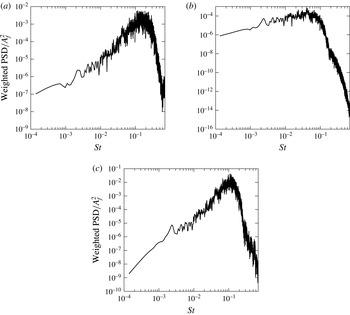
, the WPSDs exhibit a broadband amplification frequency centred at a non-dimensional frequency in the range of
 $St\in [0.05;0.5]$
for
 $P_{1}$
and
 $P_{3}$
. This selectivity is mainly due to the shear layer. Similar results are obtained for
 $P_{4}$
(not shown here). In addition, figure 15(b) shows that the measurement associated with probe
 $P_{2}$
exhibits a low-frequency broadband energy content. In this position, the linearized dynamics presents no particular selectivity and beyond
 $St\approx 0.1$
, all frequencies are attenuated. Different grids has been tested, showing that these features are independent of the numerical choices.
Linear and nonlinear regimes: forcing parameters and measurement coordinates.

 $M_{\infty }=2.15$
,
 ${\it\theta}=30.8^{\circ }$
and
 $Re_{{\it\delta}^{\star }}=1050$
(Case A). Linear regime. Frequency response to upstream broadband white noise forcing (
 $F1$
) at the (a) separating point; (b) separated shock; (c) downstream position. The WPSDs normalized by the forcing amplitude are represented as a function of the dimensionless frequency (
 $St$
). (a)
 $P_{1}$
– separating point, (b)
 $P_{2}$
– separated shock, (c)
 $P_{3}$
– separated zone.

 $M_{\infty }=2.15$
,
 ${\it\theta}=30.8^{\circ }$
and
 $Re_{{\it\delta}^{\star }}=1050$
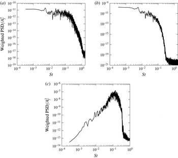
(Case A). Linear regime. Frequency response to internal broadband white noise forcing (
 $F2$
) at the (a) separating point; (b) separated shock; (c) downstream position. The WPSDs normalized by the forcing amplitude are represented as a function of the dimensionless frequency (
 $St$
). (a)
 $P_{1}$
– separating point, (b)
 $P_{2}$
– separated shock, (c)
 $P_{4}$
– downstream point.

For the internal broadband white noise forcing,
 $F2$
, the WPSDs have a low-frequency broadband content with no particular selectivity for
 $P_{1}$
and
 $P_{2}$
.
 $P_{3}$
and
 $P_{4}$
display a selective-frequency response similar to the
 $F1$
case. In addition, it is interesting to note that when the forcing is localized near the separation point, the amplitude of the response is larger than the one associated with forcing
 $F2$
(i.e. inside the bubble). These results are in agreement with those of Sansica et al. (Reference Sansica, Sandham and Hu2014), only the frequency range involved is different and can be largely explained by an effect of the Mach number (1.5 in their case). To characterize the spatial shape of structures for a single frequency associated with the response to a white noise forcing, 10 000 every
 ${\rm\Delta}t{\it\delta}^{\star }/U_{e}=0.148$
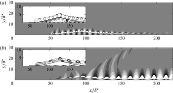
of streamwise velocity and pressure fluctuation snapshots are stored and Fourier transformed. In figure 17(a,b), Fourier modes corresponding to
 $St\approx 0.145$
and
 $St\approx 0.056$
are represented for case A. On the one hand, figure 17(a) shows that most amplified frequencies are associated with not radiating Kelvin–Helmholtz modes reminiscent of subsonic Kelvin–Helmholtz global modes. On the other hand, low-frequency Fourier modes exhibit a spatial amplification of vortices along the separated zone with emission of an acoustic wave into the expansion fan, similar to supersonic Kelvin–Helmholtz global modes. To further illustrate this, the Fourier modes are projected into a set of global modes using an orthogonal projection that relies on Gram–Schmidt orthonormalization. The procedure is detailed in Song et al. (Reference Song, Alizard, Robinet and Gloerfelt2013). Hence, a single Fourier mode may be decomposed as
 $$\begin{eqnarray}\boldsymbol{q}_{Fourier}(x,y)=\mathop{\sum }_{i=1}^{N}W_{i}\hat{\boldsymbol{q}}_{i}(x,y),\end{eqnarray}$$
with
 $W_{i}$
being the coefficient of projection onto the global mode
 $\hat{\boldsymbol{q}}_{i}$
. Hereafter,
 $N=100$
global modes are considered. The weighted spectra are shown in figure 18(a,b). The figures show that, while the Fourier mode associated with
 $St\approx 0.145$
involves mainly global modes associated with regions II and III, the global modes of region I concentrate more energy for the Fourier mode corresponding to
 $St\approx 0.056$
, consistent with the acoustic radiation observed in figure 17(a). Consequently, it is clear from figure 17(a,b) that Fourier modes may be considered to be a train of wavepackets beating to a single frequency given by the Fourier transform. In particular, the latter wavepackets are composed of many frequency components, each of them being associated with a global mode. In addition, figure 17(a,b) also show the consequence of dispersive effects associated with boundary-layer modes and Kelvin–Helmholtz modes (region I, II and III, respectively) that travel with different phase velocities. In particular, one may observe that the wavepacket spreads out for low frequencies in comparison to medium frequencies (as depicted in figure 17
a,b). From the discussion above, it seems clear that OSWBLI filters and amplifies a specific range of frequencies, characteristic of a selective noise amplifier (Sipp et al.
Reference Sipp, Marquet, Méliga and Barbagallo2010) and also give a physical explanation of individual global modes as a wavepacket component. The Fourier analysis shows that actuation in the vicinity of the separation provides a more efficient response for the most amplified frequencies than an actuation inside the separation zone. Hence, one may conclude that subsonic Kelvin–Helmholtz global modes have greater receptivity near the separation point whereas supersonic Kelvin–Helmholtz global modes are more receptive to a forcing localized inside the bubble. In addition, the predominance of supersonic Kelvin–Helmholtz global modes for Fourier modes with
 $St\approx 0.056$
provide physical insight useful to the interpretation of the amplification of lower frequencies measured with
 $P_{2}$
as shown in figures 15(b) and 16(b). Indeed, in the region near the probe
 $P_{2}$
, the flow is mainly driven by acoustic disturbances which are associated with supersonic Kelvin–Helmholtz modes.
 $M_{\infty }=2.15$
,
 ${\it\theta}=30.8^{\circ }$
and
 $Re_{{\it\delta}^{\star }}=1050$
(Case A). Linear regime. Fourier analysis: contours of the pressure fluctuations for (a) mode with
 $St\approx 0.145$
(i.e.
 $St\times L_{int}/{\it\delta}^{\star }=5.52$
) and (b) mode with
 $St\approx 0.056$
(i.e.
 $St\times L_{int}/{\it\delta}^{\star }=2.05$
). In the subfigures, the corresponding spanwise vorticity is represented.

 $M_{\infty }=2.15$
,
 ${\it\theta}=30.8^{\circ }$
and
 $Re_{{\it\delta}^{\star }}=1050$
(Case A). Linear regime. Contributions of individual global modes to (a) the single Fourier mode associated with
 $St\approx 0.145$
(see figure 17
a) and (b) the single Fourier mode associated with
 $St\approx 0.056$
(see figure 17
b). The circles are proportional to the corresponding expansion coefficients associated with the projection of the Fourier modes (referenced as
 $W_{i}$
in (4.4)).

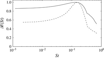
The frequency selection observed in figures 15(a,c) and 16(a,c), can be explained in a global framework through the analysis of the global resolvent,
 ${\mathcal{R}}({\it\omega})$
(see Sipp et al. (Reference Sipp, Marquet, Méliga and Barbagallo2010) for the technical details). The latter quantity represents the maximum response of the flow due to a harmonic forcing at a frequency
 ${\it\omega}$
and is strongly associated with the non-orthogonality of the global modes.
 ${\mathcal{R}}({\it\omega})$
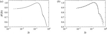
can be approximated by using the Hessenberg matrix from the Arnoldi algorithm (see Toh & Trefethen Reference Toh and Trefethen1996). The relevancy of our approach is discussed in § A.2. In figure 19, the distribution of
 ${\mathcal{R}}$
is shown as a function of the non-dimensional frequency
 $St$
for flow cases A and C. Apart from the amplification of a wide range of frequencies in between, the latter curve exhibits a maximum for
 $St\approx 0.145$
consistent with the linear simulation. In addition, the most amplified Strouhal number is seen to be not affected by an increase of
 ${\it\theta}$
from 30.8° to 32°. This result is in agreement with the scaling for the global spectra analysed in the previous section.
Distribution of the global resolvent as a function of the dimensionless frequency
 $St$
for case A (full line) and case C (dashed lines). The maximum amplitude of
 ${\mathcal{R}}$
is defined up to a multiplicative constant.

4.4. Influence of nonlinearities
 $M_{\infty }=2.15$
,
 ${\it\theta}=30.8^{\circ }$
and
 $Re_{{\it\delta}^{\star }}=1050$
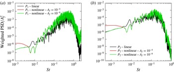
(Case A). Frequency response to upstream broadband white noise forcing for nonlinear Navier–Stokes equations. (a)
 $P_{1}$
– separating point, (b)
 $P_{2}$
– separated shock.

 $M_{\infty }=2.15$
,
 ${\it\theta}=30.8^{\circ }$
and
 $Re_{{\it\delta}^{\star }}=1050$
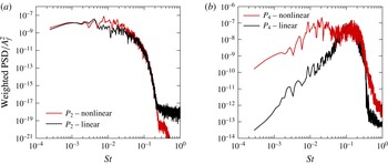
(Case A). Frequency response to internal broadband white noise forcing for nonlinear Navier–Stokes equations. (a)
 $P_{2}$
– separated shock, (b)
 $P_{4}$
– downstream.

To give insight into the influence of nonlinearities, we investigate the nonlinear response to a white noise forcing for case A. For that purpose, the same forcing as the one described in the previous section is used. Besides the linear regime, different simulations with various amplitudes are carried out. In particular,
 $A_{f}=10^{-8}$
and
 $A_{f}=10^{-4}$
are considered for
 $F1$
and
 $A_{f}=10^{-6}$
is considered for
 $F2$
. In figure 20, the WPSDs associated with
 $F1$
are reported for the probes
 $P_{1}$
and
 $P_{2}$
. It is interesting to note that the frequency selection observed in the linear regime is not strongly affected by nonlinearities. In particular, WPSDs associated with the probe
 $P_{1}$
exhibit an energy peak close to
 $St\approx 0.14$
and a wide range of amplified frequencies between
 $St\approx 0.05$
and
 $St\approx 0.5$
for both
 $A_{f}=10^{-8}$
and
 $A_{f}=10^{-4}$
, in agreement with the linear frequency response. However, the figure 20 also shows that low frequencies are energetically more significant when the forcing amplitude is increased for both
 $P_{1}$
and
 $P_{2}$
. This suggests a stronger selectivity of the lower frequency when nonlinearities have a significant contribution. These results are compatible with the results obtained by Sansica et al. (Reference Sansica, Sandham and Hu2014). However, in their work, the influence of nonlinearity is more pronounced because the interaction zone is larger which yields intense nonlinear dynamics of the shear layer. The WPSDs associated with
 $F_{2}$
are displayed in figure 21. In (a), the figure shows that the frequency response associated with pressure measurements in
 $P_{2}$
are not affected by nonlinearities. Similar results are obtained for
 $P_{1}$
. In (b), one may observe an increase of the energy content over the low frequencies when increasing the forcing amplitude inside the recirculation zone. On the one hand, this suggests that the nonlinear receptivity to frequencies associated with regions I and II (see spectrum 8) exhibit a similar behaviour as the one discussed in the section devoted to the linear regime. In particular, while the nonlinear receptivity of frequencies for region II are localized near the separation point, frequencies for region I have a greater receptivity to a forcing inside the recirculation zone. On the other hand, it is clear from the figure 21(b) that nonlinearities tend to increase this behaviour. Finally, in figure 22, the Fourier mode associated with
 $St=0.02$
(
 $St\times L_{int}/{\it\delta}^{\star }\approx 0.73$
) is represented. As for the linear regime, we may observe that its spatial support is mainly localized in the separated region. This indicates that nonlinearities tend to favour the emergence of low-frequency modes strongly associated with the recirculation zone. We can also remark that no acoustic radiation is observed in figure 22(a). This thus provides evidence that the mechanism associated with the nonlinear Fourier mode shown in figure 21 is distinct from the one linked to the supersonic Kelvin–Helmholtz modes observed in the linear regime.
Case A: nonlinear regime. Fourier mode for
 $St=0.02$
. (a) The pressure component. (b) The spanwise vorticity component. The black solid line denotes a streamline above the separation line.

5. Discussion and conclusion
The interaction between an oblique impinging shock wave and laminar boundary layer developing on a flat plate has been analysed using a linear stability approach and numerical simulations. This study was carried out for different values of the incident shock angle, Reynolds and Mach numbers. The stability analysis has shown that OSWBLIs are globally stable for this range of parameters. In particular, the global spectrum involves a wide variety of global modes that are identified and catalogued. Kelvin–Helmholtz modes, describing the perturbation dynamics along the shear layer, are observed to fall into two categories: one where Mach-waves are radiated in the free stream (called supersonic Kelvin–Helmholtz modes) and one that is characterized by waves that propagate with a subsonic relative phase velocity (called subsonic Kelvin–Helmholtz modes). Boundary-layer modes are also identified, dominated by structures mainly located in the attached region. Finally, global modes dominated by acoustic waves (i.e. propagating at the speed of sound) in the free stream are also found. In addition, when the Reynolds and Mach numbers are kept almost constant (
 $M_{\infty }\approx 2.15$
and
 $Re_{{\it\delta}^{\star }}\approx 1000$
), it is seen that characteristic frequencies for subsonic and supersonic Kelvin–Helmholtz modes exhibit a universal behaviour when using a scaling based either on the interaction length or the displacement thickness at the impact of the incident shock, not dependent on the bubble’s shape. This scaling is seen to be Reynolds number and/or Mach number dependent but further investigations at various Mach numbers and Reynolds numbers are needed in order to make a firm statement on this point. The main consequence is that the OSWBLI behaves as a selective noise amplifier and its dynamics is driven mainly by receptivity mechanisms and a non-modal transient response. To further illustrate this behaviour, we have exploited the global modes and carried out numerical simulations of forced OSWBLI for the case
 $M_{\infty }=2.15$
and
 $Re_{{\it\delta}^{\star }}=1050$
(also referred to as the Degrez’s case). The global stability analysis has revealed that the spatial scales responsible for the Strouhal number range
 $St\in [0.05,0.5]$
are localized mainly in the interaction zone. The lower the frequency, the more the perturbations at the origin of these frequencies are located in the separated shock and shear-layer foots. The global resolvent has shown that the frequency response is multi-modal with a selectivity around
 $St\in [0.05,0.5]$
and a peak close to 0.14 (we recall that
 $St$
is based on
 ${\it\delta}^{\star }$
and
 $U_{e}$
). No particular selectivity is observed at low frequency. In order to clarify the receptivity mechanisms, Degrez’s case has been locally forced upstream (respectively downstream) to the OSWBLI. The linear and nonlinear response of the flow has been analysed at some chosen points. The linear forcing confirmed the stability analysis results and the most amplified frequencies exhibit good agreement with the shape of the global resolvent. Nonlinear dynamics has shown two different response families. For the medium and high frequencies,
 $St\in [0.05,0.5]$
, the nonlinear dynamics is qualitatively close to the linear response. It corresponds to the dynamics of the shear layer, where Kelvin–Helmholtz-type instabilities develop. In contrast, the low-frequency dynamics,
 $St\in [5\times 10^{-4},0.05]$
, is qualitatively different to the linearized one. When the amplitude of the forcing or the interaction intensity are strong enough, the amplitude of the response is higher in comparison with the linear dynamics. An underlying nonlinear mechanism appears to be responsible for this behaviour. Sansica et al. (Reference Sansica, Sandham and Hu2014) indicate that this low-frequency response can be driven by the nonlinearities of the shear layer at the reattachment point. Such a mechanism has already been found for separated subsonic flows where self-sustained low-frequency oscillations are observed for a large separation zone (Dovgal, Kozlov & Michalke Reference Dovgal, Kozlov and Michalke1994; Ehrenstein & Gallaire Reference Ehrenstein and Gallaire2008).
Concerning the scenarios discussed in the introduction, none of these can be definitely ruled out. The selective-amplifier character of the OSWBLI for two-dimensional disturbances does not exclude a forcing of upstream disturbances (Ganapathisubramani et al. Reference Ganapathisubramani, Clemens and Dolling2007). However, we have shown that a forcing in the interaction zone is more effective than an upstream one. Concerning the scenario linked to an acoustic feedback loop (Pirozzoli & Grasso Reference Pirozzoli and Grasso2006), we have highlighted various acoustic emission mechanisms, yet none of them can explain the two orders of magnitude between the main flow dynamics (vortex shedding or shear-layer instabilities) and the dynamics of the separated shock. The scenario proposed by Piponniau et al. (Reference Piponniau, Dussauge, Debieve and Dupont2009) is only indirectly connected to the instabilities of the shear layer. It postulates that the low frequencies are the result of a rebalancing mechanism between the loss of mass carried by vortices developing in the shear layer and its basic state (the equilibrium state of the undisturbed separated zone). At this stage it is unclear whether the model of Piponniau et al. matches the nonlinear mechanism observed in this study. As for the Touber’s scenario (Touber & Sandham Reference Touber and Sandham2011), it is not inconsistent with our results. To better discriminate among these scenarios, it is necessary to further study the different nonlinear mechanisms which may be responsible for the low-frequency dynamics.
Our analysis seems also to establish a strong coupling between the dynamics of the separated zone and the low-frequency dynamics. In particular, this link seems to have a nonlinear origin consistent with the results given by Sansica et al. (Reference Sansica, Sandham and Hu2014). An interesting synthesis of these different scenarios is given by Morgan et al. (Reference Morgan, Duraisamy, Nguyen, Kawai and Lele2013).
Although this paper focuses on a strictly laminar interaction, some clues can be given to better understand the turbulent interaction. Numerical simulations realized by Touber & Sandham (Reference Touber and Sandham2009b
), Priebe & Martin (Reference Priebe and Martin2012) and Aubard et al. (Reference Aubard, Gloerfelt and Robinet2013) highlight a dynamics qualitatively similar to that of a laminar flow. Two frequency scales appear clearly,
 $St_{L_{int}}\approx 0.5$
and
 $St_{L_{int}}\approx 0.03$
, matching the dynamics of the shear layer and the shock of separation, respectively. However, some quantitative differences are observed. The most obvious difference lies in the scale ranges set in. In the laminar regime, the Strouhal numbers range related to the shear-layer dynamics is around
 $St_{L_{int}}\approx 5$
while in the turbulent regime is close to
 $St_{L_{int}}\approx 0.5$
. This difference implies that the instabilities in the turbulent OSWBLI have larger wavelengths than those in the laminar case. This difference can be explained by the different values of the displacement thickness (or vorticity thickness). For example; a comparison between Degrez and IUSTI cases gives:
 $(L_{int}/{\it\delta}^{\star })_{lam}\simeq 36.7$
and
 $(L_{int}/{\it\delta}^{\star })_{tur}\simeq 13.2$
and
 ${\it\delta}_{tur}^{\star }/{\it\delta}_{lam}^{\star }\simeq 5$
.
Both numerical simulations and experiments of turbulent OSWBLI indicate a smaller mean separated zone compared to the one observed in a laminar case. With regards to the convective/absolute transition criterion based on the reversed-flow velocity (see Hammond & Redekopp Reference Hammond and Redekopp1998), it suggests a convective nature of instabilities developing in the interaction zone. In addition, the separated zone of turbulent OSWBLI is continuously forced by turbulent structures. It may thus be supposed that the origin of low-frequency unsteadiness in the turbulent regime is also associated with the nonlinear interaction between instability modes arising in the shear layer, as shown for the laminar case in the present study.
However, based on the assumption that coherent structures are uncorrelated to the disorganized ones, recent global stability analyses carried out on a mean turbulent flow (Sartor et al. Reference Sartor, Mettot, Sipp and Bur2013; Sartor Reference Sartor2014) suggest that low-frequency unsteadiness in transonic turbulent shock wave/boundary-layer interaction cannot be explained by the presence of unstable global modes, and is mainly driven by a linear pseudo-resonance mechanism. Hence, it should be an interesting prospect to perform a similar analysis for the turbulent OSWBLI to give a more definitive statement.
Furthermore, our analysis is restricted to two-dimensional disturbances. Robinet (Reference Robinet2007) has highlighted that a laminar OSWBLI could become globally unstable with respect to three-dimensional disturbances, leading to a bifurcation from a 2-D steady state to a 3-D steady state. However, convective instabilities may induce an abrupt transition to turbulence and can ‘bypass’ this global mechanism. For supersonic flow, Mack (Reference Mack1969) has found that the most unstable convective waves are three-dimensional. Pagella et al. (Reference Pagella, Rist and Wagner2002) and Yao et al. (Reference Yao, Krishnan, Sandham and Roberts2007) have shown that these instabilities can play an important role in mechanisms of transition to turbulence in a laminar OSWBLI. In future work, it would be interesting to study the global stability and receptivity process of an OSWBLI with respect to 3-D perturbations.
Acknowledgements
This work was supported through the French Centre National d’Études Spatiales (CNES) and the Direction Générale de l’Armement (DGA) and was conducted as part of ATAC (Aérodynamique des Tuyères des Arrières-Corps) Group. The authors would like to thank Supersonic group at IUSTI and more globally the members of ANR DECOMOS project for fruitful conversations.
Appendix A. Numerical validations
A.1. Eigenspectrum
To test the robustness of the eigenspectrum for case A, two other grids are studied
 $(N_{x}\times N_{y})=(650\times 100)$
and
 $N_{x}\times N_{y}=900\times 200$
. Figure 23 shows the eigenspectra obtained with the reference grid (the one used in the paper) and the other resolutions.
In figure 23, we may observe that results carried out on
 $(N_{x}\times N_{y})=(560\times 100)$
and
 $(N_{x}\times N_{y})=(650\times 100)$
are almost undistinguishable. However, when comparing with the finest resolution, significant differences occur for the highest frequencies (above
 $St\approx 0.16$
). This suggests a very slow convergence of the spectrum for this part of the spectrum. It is also consistent with the fact that higher frequencies are associated with smaller scales and are better discretized with the finest grid. However, the characteristic scales (i.e. the frequency peak around
 $St\approx 0.14$
and the separation between subsonic and supersonic Kelvin–Helmholtz modes around
 $St\times L_{int}/{\it\delta}^{\star }\approx 2.8$
) are not really modified when increasing the number of grid points from the reference grid. In addition, modes corresponding to frequencies above
 $St\approx 0.16$
are not quite involved in the space dynamics of OSWBLI as shown in figure 18 where a projection of the flow response onto a set of global modes is performed. Hence, the reference grid can be considered a good compromise between resolution and a reasonable computational time.
 $M_{\infty }=2.15$
,
 ${\it\theta}=30.8^{\circ }$
and
 $Re_{{\it\delta}^{\star }}=1050$
(case A). ● (reference grid):
 $(N_{x}\times N_{y})=(560\times 100)$
; ▪:
 $(N_{x}\times N_{y})=(650\times 100)$
;
 $\star$
:
 $(N_{x}\times N_{y})=(900\times 200)$
.

Furthermore, the slow convergence for the global spectrum can be explained by the
 ${\it\varepsilon}$
-pseudospectrum and not only by a lack of spatial resolution. A current definition of the
 ${\it\varepsilon}$
-pseudospectrum is given by
 $$\begin{eqnarray}{\it\Lambda}_{{\it\varepsilon}}=\{{\it\omega}\in \mathbb{C}:\Vert {\mathcal{R}}({\it\omega})\Vert >{\it\varepsilon}^{-1}\}.\end{eqnarray}$$
The pseudo-spectrum can also be interpreted as
 $\Vert {\mathcal{R}}({\it\omega})\Vert \geqslant 1/\text{dist}[z,Sp(J)]$
where
 $z$
is a point in complex plane and
 $\text{dist}[z,Sp(J)]$
denotes the distance between
 $z$
and the spectrum (Sp) of the Jacobian
 $J$
. The pseudospectrum gives a measure of the potential change in the eigenvalues once the Jacobian operator is perturbed by an operator
 ${\mathcal{P}}$
of norm
 ${\it\varepsilon}$
(see Trefethen & Embree Reference Trefethen and Embree2005). It yields some useful information about the robustness of eigenvalues to the numerical parameters. In figure 24, it can be observed that when the Jacobian operator is disturbed, for example by
 ${\it\varepsilon}\simeq 10^{-6}$
, it causes a disturbance
 ${\rm\Delta}{\it\lambda}$
of the order of
 $6\times 10^{-3}$
on the eigenvalues of the branch II. However, this same disturbance causes a
 ${\rm\Delta}{\it\lambda}\simeq 8\times 10^{-2}$
for some eigenvalues of branch III around
 $St=0.2$
. This result shows that the eigenvalues are highly sensitive to data (physical or numerical origins) disturbances related to the non-normality of the Jacobian operator. For the eigenvalues of the branch III, this sensitivity is mainly of numerical origin, these modes are associated with the boundary layer downstream and are exponentially amplified in the streamwise direction. The envelope of these modes is not contained in the computational domain (unless we have a very large domain, which is too expensive numerically), the influence of the downstream boundary condition is not negligible for these modes.
 ${\it\varepsilon}$
-pseudospectrum for the case A:
 $M_{\infty }=2.15$
,
 ${\it\theta}=30.8^{\circ }$
and
 $Re_{{\it\delta}^{\star }}=1050$
. The grid used is
 $(N_{x}\times N_{y})=(560\times 100)$
and the domain size is
 $[0;400]\times [0;80]$
.

 $M_{\infty }=2.15$
,
 ${\it\theta}=30.8^{\circ }$
and
 $Re_{{\it\delta}^{\star }}=1050$
(Case A). Dependence on global resolvent with respect to number of snapshots
 $N_{s}$
(
 $N_{s}=320$
: full line,
 $N_{s}=360$
dashed line,
 $N_{s}=400$
dash-dot line) for the reference grid:
 $(N_{x}\times N_{y})=(560\times 100)$
.

A.2. Global resolvent
The global resolvent being computed from the pseudospectra (figure 24), it is important to check that the latter quantity is not dependent on the Krylov subspace dimension
 $N_{s}$
. In figure 25(a), we show that the resolvant curves
 ${\mathcal{R}}(St)$
computed with
 $N_{s}=320,360$
and 400 are almost undistinguishable.