





1. Introduction
Electrophoresis, the motion of a charged particle in a liquid electrolyte under an imposed electric field, is one of the oldest and most widely studied phenomena in colloidal science. Its origins trace back to the early nineteenth century, and its modern applications span the separation of biomacromolecules (Heller Reference Heller2001), the measurement of zeta potentials (Doane et al. Reference Doane, Chuang, Hill and Burda2012), microfluidic manipulation of particles and cells (Velegol et al. Reference Velegol, Garg, Guha, Kar and Kumar2016), and the characterisation of surface charge in complex environments. The central quantity is the electrophoretic mobility, defined as the ratio of the particle velocity to the applied field strength. Over the last century, a large body of theoretical, computational and experimental work has sought to understand how the mobility depends on the properties of the particle and the surrounding electrolyte. A comprehensive review of the historical development can be found in Anderson (Reference Anderson1989), and modern advances related to nonlinear electrophoresis are described in Khair (Reference Khair2022).
Much of this theoretical progress has focused on the canonical geometry of a sphere. In the limit of a thin Debye layer (
 $\kappa a \gg 1$
, where
 $a$
is the particle radius, and
 $\kappa ^{-1}$
is the Debye length), the Helmholtz–Smoluchowski formula gives the electrophoretic velocity as
 $\boldsymbol{U} = (\varepsilon _{\kern-1pt f} \zeta / \mu )\boldsymbol{E}_\infty$
, where
 $\varepsilon _{\kern-1pt f}$
is the fluid permittivity,
 $\zeta$
is the zeta potential,
 $\mu$
is the viscosity, and
 $\boldsymbol{E}_\infty$
is the applied electric field (Smoluchowski Reference Smoluchowski1921). In the opposite limit of a thick Debye layer (
 $\kappa a \ll 1$
), Hückel (Reference Hückel1924) showed that the mobility is reduced by a factor of
 $2/3$
relative to the Smoluchowski result, reflecting the balance between the electrostatic driving force and the Stokes drag. Henry (Reference Henry1931) bridged these two limits by computing the mobility at arbitrary
 $\kappa a$
within the linearised Poisson–Boltzmann (Debye–Hückel) approximation, yielding the well-known interpolation function
 $f_H(\kappa a)$
that increases monotonically from
 $2/3$
to
 $1$
. Extensions beyond the Debye–Hückel regime, accounting for the distortion of the double layer during particle motion (the so-called relaxation effect), were developed by O’Brien & White (Reference O’Brien and White1978) through a landmark numerical computation that revealed a mobility maximum at sufficiently large zeta potentials. More recent work has addressed the fully nonlinear regime at large applied fields, where the mobility itself becomes field-dependent (Khair Reference Khair2022).
A remarkable feature (and constraint for separation applications) of the Smoluchowski result is its independence of particle shape. Morrison (Reference Morrison1970) proved that the electrophoretic velocity
 $\boldsymbol{U} = (\varepsilon _{\kern-1pt f} \zeta / \mu )\boldsymbol{E}_\infty$
holds for an insulating particle of any shape, provided that the Debye layer is thin compared to all local radii of curvature, and the zeta potential is uniform. The key insight is that the velocity field
 $\boldsymbol{u} = (\varepsilon _{\kern-1pt f} \zeta / \mu )\boldsymbol{E}$
is itself irrotational and satisfies both the Stokes equation and the slip boundary condition, regardless of the particle geometry. This result was independently confirmed by Teubner (Reference Teubner1982). As a consequence, shape effects on the electrophoretic mobility can only arise when the thin-Debye-layer assumption is relaxed.
The effect of particle shape at finite Debye length has received comparatively less attention. The most complete analytical treatment is the work of Yoon & Kim (Reference Yoon and Kim1989), who obtained exact solutions for spheroidal particles by solving the linearised Poisson–Boltzmann equation in spheroidal coordinates using spheroidal wavefunctions. Their results revealed several important features. First, the mobility of a spheroid depends on its orientation relative to the applied field. For a prolate particle, motion along the symmetry axis yields a mobility different from motion perpendicular to it. Second, for certain orientations (a prolate spheroid with the field perpendicular to its axis, or an oblate spheroid with the field along its axis), the mobility is not monotonic in
 $\kappa a$
but exhibits a minimum at intermediate double-layer thicknesses, reflecting a subtle competition between electrostatic and hydrodynamic retardation forces. Third, when the mobility is averaged over all orientations (as would be measured for a randomly oriented ensemble), the result deviates only modestly from the sphere, and the orientation-averaged Hückel-limit mobility is exactly
 $2/3$
for all spheroids, regardless of aspect ratio. Beyond spheroids, computational studies have addressed the electrokinetics of rod-like and slender particles (Solomentsev & Anderson Reference Solomentsev and Anderson1994; Ohshima Reference Ohshima1996), but to the best of our knowledge, no general analytical framework exists for arbitrary shape effects on electrophoretic mobility.
The shape-independence of the Smoluchowski result implies that the question of how shape affects electrophoresis is inextricably tied to finite double-layer effects. This coupling presents a methodological challenge. Much of the modern literature on phoretic mobility calculations, particularly for self-propelled particles, relies on the slip velocity formulation popularised by Stone & Samuel (Reference Stone and Samuel1996). In this framework, the thin-Debye-layer approximation is invoked to replace the electrokinetic body force with an effective slip velocity at the particle surface, after which the velocity is obtained from a surface integral using the Lorentz reciprocal theorem. This approach is powerful and widely used (Stone & Samuel Reference Stone and Samuel1996; Masoud & Stone Reference Masoud and Stone2019), but it is restricted to thin Debye layers and therefore cannot capture shape-dependent corrections to the mobility. To study the interplay between shape and finite double-layer thickness, one must instead work with the full volume integral formulation, in which the body force throughout the fluid is retained explicitly.
In this work, we employ the unified mobility expression derived by Ganguly et al. (Reference Ganguly, Roychowdhury and Gupta2024), building on the framework of Brady (Reference Brady2021), to compute the electrophoretic mobility of a nearly spherical particle at arbitrary
 $\kappa a$
and small zeta potential. The particle surface is described by
 $r_s(\theta ) = a[1 + \varepsilon f(\theta )]$
, where
 $\varepsilon \ll 1$
, and
 $f(\theta )$
is expanded in Legendre polynomials. The perturbation to the fields is obtained via the domain perturbation technique of Brenner (Reference Brenner1964), and the correction to the Stokes flow around the deformed particle is computed analytically using a Gegenbauer streamfunction decomposition. While the results are formally valid for small deformations (
 $\varepsilon \ll 1$
), they should provide useful physical insight and motivate the broader question of shape-dependent electrophoretic mobility.
The remainder of this paper is organised as follows. In § 2, we define the problem and state the governing equations. In § 3, we carry out the perturbation analysis, and compute each contribution to the shape correction coefficient. In § 4, we present the resulting mobility corrections, and validate the results against the exact solutions of Yoon & Kim (Reference Yoon and Kim1989). In § 5, we summarise the key findings, and discuss directions for future work. Finally, we note that this work was developed with the assistance of Claude (Anthropic), as detailed in § 6.
2. Problem set-up
2.1. Geometry and physical setting
We consider a rigid, non-conducting particle immersed in a symmetric binary electrolyte of viscosity
 $\mu$
, permittivity
 $\varepsilon _{\kern-1pt f}$
, and Debye length
 $\kappa ^{-1} = (\varepsilon _{\kern-1pt f} k_B T / 2 e^2 c_0)^{1/2}$
, where
 $k_B$
is the Boltzmann constant,
 $T$
is the temperature,
 $e$
is the elementary charge, and
 $c_0$
is the bulk electrolyte concentration. The particle surface is described by
 \begin{align} r_s(\theta ) = a\bigl [1 + \varepsilon f(\theta )\bigr ], \quad f(\theta ) = \sum _{n=0}^{\infty } c_n\, P_n(\cos \theta ), \end{align}
where
 $a$
is the radius of a reference sphere,
 $\varepsilon \ll 1$
is a small dimensionless parameter characterising the amplitude of the shape deformation,
 $P_n$
are Legendre polynomials, and
 $c_n$
are order-unity coefficients. We restrict attention to axisymmetric shapes, so that the surface depends only on the polar angle
 $\theta$
measured from the axis of the applied field. The particle carries a uniform zeta potential
 $\zeta$
on its surface, and the analysis is conducted within the Debye–Hückel (linearised Poisson–Boltzmann) approximation,
 $e\zeta / k_B T \ll 1$
. A uniform electric field
 $\boldsymbol{E}_\infty = E_\infty \hat {\boldsymbol{e}}_z$
is applied far from the particle. The geometry is illustrated in figure 1.
Geometry of the problem. A nearly spherical particle with surface
 $r_s(\theta ) = a[1 + \varepsilon f(\theta )]$
(lighter shade) is immersed in an electrolyte with Debye length
 $\kappa ^{-1}$
(outer shaded region). The darker circle indicates the reference sphere of radius
 $a$
. The applied electric field
 $\boldsymbol{E}_\infty$
is directed along the
 $z$
-axis. The particle carries a uniform zeta potential
 $\zeta$
.

2.2. Governing equations
Under the assumptions stated above (small
 $\zeta$
, weak applied field, negligible ionic Péclet number), the electrokinetic problem decomposes into three independent sub-problems (Henry Reference Henry1931; O’Brien & White Reference O’Brien and White1978; Ganguly et al. Reference Ganguly, Roychowdhury and Gupta2024): (i) the equilibrium double-layer potential
 $\psi$
, (ii) the applied-field potential
 $\varPhi$
, and (iii) the fluid velocity driven by the resulting body force. The equilibrium double-layer potential
 $\psi$
satisfies the linearised Poisson–Boltzmann equation
 \begin{align}{\nabla} ^2 \psi = \kappa ^2 \psi \quad \text{in} \ r \gt r_s, \end{align}
with
 $\psi = \zeta$
on
 $r = r_s$
, and
 $\psi \to 0$
as
 $r \to \infty$
. We adopt the constant surface potential condition here; an equivalent formulation specifies a constant surface charge density
 $\sigma$
via Gauss’s law,
 $-\varepsilon _{\kern-1pt f} \, \partial \psi /\partial n|_{r_s} = \sigma$
. For the weak-field electrophoresis problem in the linearised regime, O’Brien & White (Reference O’Brien and White1978) showed that the mobility is independent of whether one specifies constant potential or constant charge, a point also noted by Yoon & Kim (Reference Yoon and Kim1989) for spheroids, and by Ganguly et al. (Reference Ganguly, Roychowdhury and Gupta2024) for arbitrary particle shapes. The two formulations therefore yield identical results for the shape corrections computed in this work; for a recent and detailed comparison of the constant-potential and constant-charge formulations, including the nonlinear high-potential regime where this equivalence no longer holds, see Casarella et al. (Reference Casarella, Gourdin-Bertin and Chassagne2025). We note, however, that this equivalence does not extend to diffusiophoresis, where the imposed solute gradient perturbs the equilibrium ion distribution, and the surface electrostatic condition enters the mobility at leading order (Prieve et al. Reference Prieve, Anderson, Ebel and Lowell1984; Gupta et al. Reference Gupta, Rallabandi and Stone2019). Thus while the electrophoretic results of this paper are insensitive to the choice of boundary condition, a generalisation to diffusiophoresis would require specifying the surface condition explicitly.
The potential associated with the applied electric field,
 $\varPhi$
, satisfies Laplace’s equation:
 \begin{align} {\nabla} ^2 \varPhi = 0 \quad \text{in}\quad r \gt r_s, \end{align}
with the insulating boundary condition
 $\partial \varPhi / \partial n = 0$
on
 $r = r_s$
, and
 $\varPhi \to -E_\infty r \cos \theta$
as
 $r \to \infty$
. Following Brady (Reference Brady2021) and Ganguly et al. (Reference Ganguly, Roychowdhury and Gupta2024), the fluid motion is driven by an osmophoretic body force
 \begin{align} {\boldsymbol{b}} = \varepsilon _{\kern-1pt f} \kappa ^2 \psi \boldsymbol{\nabla }\kern-1pt\varPhi , \end{align}
which arises at leading order in the Debye–Hückel limit for a symmetric electrolyte. The body force is concentrated in the diffuse double layer, where the equilibrium charge density
 $\rho _e = -\varepsilon _{\kern-1pt f} \kappa ^2 \psi$
is non-zero. We emphasise that the decomposition into
 $\psi$
and
 $\varPhi$
is a consequence of the weak-field (linear) approximation and holds at arbitrary
 $\kappa a$
.
2.3. Unified mobility expression
The translational velocity of the particle is obtained from a reciprocal theorem framework. For a particle of arbitrary shape, the result reads
 \begin{align} \boldsymbol{U} = \boldsymbol{M}_{\textit{UF}} \boldsymbol{\cdot }\int _V (\boldsymbol{D}^{\rm T} - \boldsymbol{I}) \boldsymbol{\cdot }{\boldsymbol{b}} \, \mathrm{d} V, \end{align}
where
 $\boldsymbol{M}_{\textit{UF}}$
is the hydrodynamic mobility tensor relating force to translational velocity,
 $\boldsymbol{D}^{\rm T}$
is the disturbance tensor for translation (i.e.
 $\boldsymbol{D}^{\rm T} \boldsymbol{\cdot }\hat {U}\hat {\boldsymbol{e}}_z = \hat {\boldsymbol{u}}$
, the Stokes velocity field for the particle translating with velocity
 $\hat {U}\hat {\boldsymbol{e}}_z$
), and
 $\boldsymbol{I}$
is the identity tensor. The integration is over the entire fluid volume
 $V$
exterior to the particle. The identity subtraction in
 $(\boldsymbol{D}^{\rm T} - \boldsymbol{I})$
removes the direct osmophoretic force, leaving only the hydrodynamic correction due to the disturbance flow near the particle surface. Here,
 $\hat {U}$
is an arbitrary reference speed whose value cancels in the final mobility; it serves only to define
 $\boldsymbol{D}^{\rm T}$
as a purely geometric (shape-dependent) quantity. For a sphere of radius
 $a$
,
 $\boldsymbol{M}_{\textit{UF}} = (6\pi \mu a)^{-1}\boldsymbol{I}$
, and the disturbance tensor takes the form (Kim & Karrila Reference Kim and Karrila2005)
 \begin{align} \boldsymbol{D}^{\rm T} = \frac {3a}{4r}(\boldsymbol{I} + \boldsymbol{e}_r \boldsymbol{e}_r) + \frac {a^3}{4r^3}(\boldsymbol{I} - 3\boldsymbol{e}_r \boldsymbol{e}_r), \end{align}
where
 $\boldsymbol{e}_r$
is the radial unit vector. An important property of (2.6) is that
 $\boldsymbol{D}^{\rm T} \to \boldsymbol{I}$
as
 $r \to a$
, so that
 $(\boldsymbol{D}^{\rm T} - \boldsymbol{I}) \boldsymbol{\cdot }{\boldsymbol{b}}$
vanishes on the sphere surface. This vanishing will have direct consequences for the domain correction at
 $O(\varepsilon )$
.
Projecting (2.5) onto the
 $z$
-axis, and substituting the leading-order fields on the reference sphere, recovers the classical result of Henry (Reference Henry1931),
 \begin{align} U_0 = \frac {\varepsilon _{\kern-1pt f} \zeta E_\infty }{\mu } \, f_H(\kappa a), \end{align}
where
 $f_H(\kappa a)$
is Henry’s function, which interpolates monotonically from
 $f_H(0) = 2/3$
(the Hückel limit) to
 $f_H(\infty ) = 1$
(the Smoluchowski limit). Interested readers are referred to Ganguly et al. (Reference Ganguly, Roychowdhury and Gupta2024) for a more detailed derivation of this result.
2.4. Perturbation structure
To compute the
 $O(\varepsilon )$
correction to the mobility, we expand all fields in powers of
 $\varepsilon$
:
 $\psi = \psi _0 + \varepsilon \psi _1 + {\cdots}$
,
 $\varPhi = \varPhi _0 + \varepsilon \varPhi _1 + {\cdots}$
,
 ${\boldsymbol{b}} = {\boldsymbol{b}}_0 + \varepsilon {\boldsymbol{b}}_1 + {\cdots}$
. The deformed particle also modifies the disturbance tensor
 $\boldsymbol{D}^{\rm T} = \boldsymbol{D}^{\rm T}_0 + \varepsilon \boldsymbol{D}^{\rm T}_1 + {\cdots}$
, the mobility tensor
 $\boldsymbol{M}_{\textit{UF}} = (6\pi \mu a)^{-1}(1 + \varepsilon \alpha _n^{\textit{drag}} + {\cdots} )\boldsymbol{I}$
(where
 $\alpha _n^{\textit{drag}}$
is the Brenner drag correction), and the integration domain
 $V = V_0 + \varepsilon \,\delta V + {\cdots}$
. The perturbation fields
 $\psi _1$
and
 $\varPhi _1$
are obtained by Taylor-expanding the boundary conditions from the deformed surface
 $r = r_s$
to the reference sphere
 $r = a$
, and solving the resulting boundary-value problems on the sphere, following the domain perturbation technique of Brenner (Reference Brenner1964). The perturbation to the Stokes flow,
 $\hat {\boldsymbol{u}}_1 = \boldsymbol{D}^{\rm T}_1 \boldsymbol{\cdot }\hat {U}\hat {\boldsymbol{e}}_z$
, is likewise obtained by projecting the no-slip condition onto the reference sphere.
The electrophoretic velocity at
 $O(\varepsilon )$
may be written as
 \begin{align} U = U_0 \bigl [1 + \varepsilon c_n \, \sigma _n(\kappa a) + O(\varepsilon ^2)\bigr ], \end{align}
where
 $\sigma _n(\kappa a)$
is a shape correction coefficient that depends on the Legendre mode
 $n$
and the dimensionless Debye length
 $\kappa a$
. Collecting terms at
 $O(\varepsilon )$
in (2.5) yields
 \begin{align} \sigma _n(\kappa a) = \frac {\mathcal{I}^{(\psi _1)} + \mathcal{I}^{(\varPhi _1)} + \mathcal{I}^{(\hat {\boldsymbol{u}}_1)} + \mathcal{I}^{({dom})}}{\mathcal{J}_0} + \alpha _n^{\textit{drag}}, \end{align}
where
 $\mathcal{J}_0$
is the base integral that produces Henry’s result (2.7), and the four numerator integrals arise respectively from (i) the perturbation to the equilibrium potential (
 $\psi _1$
), (ii) the perturbation to the applied field (
 $\varPhi _1$
), (iii) the perturbation to the Stokes flow (
 $\hat {\boldsymbol{u}}_1$
), and (iv) the shift in the integration domain (
 $\delta V$
). Each of these contributions has a distinct physical origin and
 $\kappa a$
-dependence, and they are evaluated in detail in § 3.
3. Mathematical derivation
We now evaluate each contribution to the shape correction coefficient
 $\sigma _n(\kappa a)$
defined in (2.9). For concreteness, we present the complete derivation for the quadrupolar mode
 $f(\theta ) = c_2\, P_2(\cos \theta )$
, which is the leading shape deformation that produces a net mobility correction. Higher modes are discussed in § 3.7.
3.1. Leading-order fields and Henry’s function
On the reference sphere, the equilibrium potential satisfying (2.2) with
 $\psi _0(a) = \zeta$
and
 $\psi _0 \to 0$
at infinity is
 \begin{align} \psi _0(r) = \zeta \frac {a}{r} \, {\rm e}^{-\kappa (r-a)}. \end{align}
The exponential decay on the scale
 $\kappa ^{-1}$
reflects the screening of the surface charge by the diffuse double layer, while the
 $a/r$
prefactor is the familiar electrostatic potential of a sphere. The applied-field potential satisfying (2.3) with
 $\partial \varPhi _0/\partial r = 0$
at
 $r = a$
, and
 $\varPhi _0 \to -E_\infty r\cos \theta$
at infinity, is
 \begin{align} \varPhi _0(r,\theta ) = -E_\infty \left (r + \frac {a^3}{2r^2}\right )\cos \theta . \end{align}
The dipole correction
 $a^3/(2r^2)$
arises from the insulating boundary condition, and enhances the tangential electric field at the particle surface by a factor
 $3/2$
relative to the imposed field.
Substituting
 ${\boldsymbol{b}}_0 = \varepsilon _{\kern-1pt f}\kappa ^2\psi _0\,\boldsymbol{\nabla }\varPhi _0$
into the
 $z$
-component of (2.5), and performing the angular integration, recovers the classical result
 $U_0 = (\varepsilon _{\kern-1pt f}\zeta E_\infty /\mu )\,f_H(\kappa a)$
, with Henry’s function given by (Henry Reference Henry1931)
 \begin{align} f_H(\kappa a) = 1 + 2\int _1^\infty \frac {{\rm e}^{-\kappa a(s-1)}}{s^5}\,\mathrm{d} s - 5\int _1^\infty \frac {{\rm e}^{-\kappa a(s-1)}}{s^7}\,\mathrm{d} s, \end{align}
where
 $s = r/a$
. In the thick-double-layer limit (
 $\kappa a \to 0$
), the exponential factor approaches unity throughout the fluid, and the integrals evaluate to
 $1/4$
and
 $1/6$
, yielding
 $f_H(0) = 1 + 1/2 - 5/6 = 2/3$
(the Hückel result). In the thin-double-layer limit (
 $\kappa a \to \infty$
), the exponential factor
 ${\rm e}^{-\kappa a(s-1)}$
confines both integrands to
 $s \approx 1$
, where
 $1/s^5 \approx 1/s^7 \approx 1$
, so each integral reduces to
 $\int _1^\infty {\rm e}^{-\kappa a(s-1)}\,\mathrm{d} s = 1/(\kappa a)$
, and
 $f_H \to 1 + 2/(\kappa a) - 5/(\kappa a) = 1 - 3/(\kappa a)$
, recovering the Smoluchowski result
 $f_H = 1$
at leading order, with a first correction
 $-3/(\kappa a)$
at finite
 $\kappa a$
.
For the perturbation analysis, it is useful to define the base integral
 \begin{align} \mathcal{J}_0 = 2\pi a^3 \int _1^\infty \frac {{\rm e}^{-\kappa a(s-1)}}{s}\left (\frac {2\tilde {A}}{3} + \frac {4\tilde {B}}{3}\right )s^2\,\mathrm{d} s, \end{align}
which is the volume integral producing
 $U_0$
, with the angular kernel functions
 \begin{align} \tilde {A}(s) = -\left (1-\frac {1}{s^3}\right )\left (1 - \frac {3}{2s} + \frac {1}{2s^3}\right ), \quad \tilde {B}(s) = \left (1+\frac {1}{2s^3}\right )\left (1 - \frac {3}{4s} - \frac {1}{4s^3}\right ). \end{align}
These arise from the
 $z$
-projection of
 $[(\boldsymbol{D}^{\rm T}_0 - \boldsymbol{I})\boldsymbol{\cdot }{\boldsymbol{b}}_0]_z = \varepsilon _{\kern-1pt f}\kappa ^2\psi _0 E_\infty [\tilde {A}(s)\cos ^2\theta + \tilde {B}(s)\sin ^2\theta ]$
, where the factors
 $\cos ^2\theta$
and
 $\sin ^2\theta$
come from projecting the body force components (
 $b_r\cos \theta$
and
 $b_\theta \sin \theta$
) onto
 $\boldsymbol{e}_z$
through the
 $(\boldsymbol{D}^{\rm T}_0 - \boldsymbol{I})$
kernel. Both kernel functions vanish at
 $s = 1$
,
 $\tilde {A}(1) = \tilde {B}(1) = 0$
, consistent with the property
 $(\boldsymbol{D}^{\rm T}_0 - \boldsymbol{I})|_{r=a} = \boldsymbol{0}$
noted in § 2.
3.2. Perturbation to the equilibrium potential
The deformed surface carries the same potential
 $\zeta$
, so the boundary condition
 $\psi (r_s) = \zeta$
must hold to all orders in
 $\varepsilon$
. Taylor-expanding from
 $r = r_s$
to
 $r = a$
at
 $O(\varepsilon )$
gives
 \begin{align} \psi _1(a,\theta ) = -ac_2\,P_2(\cos \theta ) \left .\frac {\partial \psi _0}{\partial r}\right |_{r=a} = \zeta c_2\,(1+\kappa a)\,P_2(\cos \theta ), \end{align}
where we have used
 $\partial \psi _0/\partial r|_{r=a} = -\zeta (1+\kappa a)/a$
from (3.1). Physically, the boundary value of
 $\psi _1$
is large when
 $\kappa a \gg 1$
because the equilibrium potential drops steeply near the surface; shifting the surface by a small amount
 $\varepsilon a$
produces a perturbation of order
 $\varepsilon \kappa a$
relative to
 $\zeta$
. The perturbation expansion is therefore well-ordered only when
 $\varepsilon \kappa a \ll 1$
, i.e. when the surface deformation is small compared to the Debye length. We note, however, that the final result for
 $\sigma _2(\kappa a)$
does recover the correct Smoluchowski limit
 $\sigma _2 \to 0$
as
 $\kappa a \to \infty$
(§ 3.8.2), so the shape correction vanishes precisely in the regime where the ordering constraint is most severe. Nonetheless, this constraint should not be overlooked when applying the theory at large but finite
 $\kappa a$
.
The perturbation
 $\psi _1$
satisfies the same linearised Poisson–Boltzmann equation,
 ${\nabla} ^2\psi _1 = \kappa ^2\psi _1$
, in
 $r \gt a$
, with
 $\psi _1 \to 0$
at infinity. The solution is
 \begin{align} \psi _1(r,\theta ) = \zeta c_2\,(1+\kappa a)\,\frac {k_2(\kappa r)}{k_2(\kappa a)}\,P_2(\cos \theta ), \end{align}
where
 $k_n(x) = \sqrt {\pi /(2x)}\,K_{n+1/2}(x)$
is the modified spherical Bessel function of the second kind, which is the unique solution of
 $({\nabla} ^2 - \kappa ^2)\phi = 0$
with
 $P_n(\cos \theta )$
angular dependence that decays at infinity. The ratio
 $k_2(\kappa r)/k_2(\kappa a)$
can be evaluated numerically using standard library functions for
 $K_{n+1/2}$
(e.g. scipy.special.kv).
The contribution of
 $\psi _1$
to the mobility correction arises from the body force perturbation
 $\varepsilon _{\kern-1pt f}\kappa ^2\psi _1\boldsymbol{\nabla }\varPhi _0$
, projected through the
 $(\boldsymbol{D}^{\rm T}_0 - \boldsymbol{I})$
kernel. Since
 $\psi _1 \propto P_2(\cos \theta )$
and the kernel functions
 $\tilde {A}(s)\cos ^2\theta + \tilde {B}(s)\sin ^2\theta$
contain only
 $P_0$
and
 $P_2$
angular components (because
 $\cos ^2\theta = (2P_2+1)/3$
and
 $\sin ^2\theta = 2(1-P_2)/3$
), the angular integral reduces by Legendre orthogonality to
 \begin{align} \mathcal{I}^{(\psi _1)} = 2\pi a^3\,(1+\kappa a)\int _1^\infty \frac {k_2(\kappa a s)}{k_2(\kappa a)}\,\frac {4(\tilde {A}-\tilde {B})}{15}\,s^2\,\mathrm{d} s. \end{align}
The angular projection coefficient
 $4(\tilde {A} - \tilde {B})/15$
arises from
 $(2/3)\int _0^\pi P_2^2\sin \theta \,\mathrm{d}\theta = 4/15$
. The radial integral is evaluated numerically using Gauss quadrature, exploiting the exponential decay of
 $k_2(\kappa a s)$
at large
 $s$
.
This result has an important corollary. For any shape mode
 $n \neq 0, 2$
, the angular integral
 $\int _0^\pi P_n\,[\tilde {A}\cos ^2\theta + \tilde {B}\sin ^2\theta ]\sin \theta \,\mathrm{d}\theta$
vanishes by orthogonality, since the integrand contains only
 $P_0$
and
 $P_2$
angular components. Therefore, the
 $\psi _1$
contribution to
 $\sigma _n$
vanishes identically for all
 $n \geqslant 3$
(and for
 $n = 1$
, which corresponds to a rigid translation and is not a genuine shape deformation).
3.3. Perturbation to the applied field
The insulating boundary condition on the deformed surface requires more care than the Dirichlet condition for
 $\psi$
, because the outward unit normal to
 $r = r_s(\theta )$
is tilted relative to
 $\boldsymbol{e}_r$
at
 $O(\varepsilon )$
. For
 $r_s = a[1 + \varepsilon f(\theta )]$
, the outward normal is
 \begin{align} \boldsymbol{n} = \boldsymbol{e}_r - \varepsilon \,f'(\theta )\,\boldsymbol{e}_\theta + O(\varepsilon ^2), \end{align}
where
 $f' = \mathrm{d} f/\mathrm{d}\theta$
. Expanding the condition
 $\boldsymbol{n}\boldsymbol{\cdot }\boldsymbol{\nabla }\varPhi |_{r_s} = 0$
to
 $O(\varepsilon )$
yields two contributions – one from Taylor-expanding
 $\partial \varPhi _0/\partial r$
from
 $r_s$
to
 $r = a$
, and one from the tilted normal acting on
 $\varPhi _0$
. Together, they give
 \begin{align} \left .\frac {\partial \varPhi _1}{\partial r}\right |_{r=a} = -a\,f(\theta )\left .\frac {\partial ^2\varPhi _0}{\partial r^2}\right |_{r=a} + \frac {f'(\theta )}{a}\left .\frac {\partial \varPhi _0}{\partial \theta }\right |_{r=a}. \end{align}
From (3.2), the required derivatives at
 $r = a$
are
 \begin{align} \left .\frac {\partial ^2\varPhi _0}{\partial r^2}\right |_{r=a} = -\frac {3E_\infty \cos \theta }{a}, \quad \left .\frac {\partial \varPhi _0}{\partial \theta }\right |_{r=a} = \frac {3}{2}\,E_\infty a\sin \theta . \end{align}
For
 $f(\theta ) = c_2\, P_2(\cos \theta )$
, we have
 $f'(\theta ) = -3c_2\sin \theta \cos \theta$
, and (3.10) becomes
 \begin{align} \left .\frac {\partial \varPhi _1}{\partial r}\right |_{r=a} = 3c_2 E_\infty P_2\cos \theta - \frac {9}{2}\,c_2 E_\infty \sin ^2\theta \cos \theta . \end{align}
The first term is
 $3c_2 E_\infty P_2\cos \theta$
, which arises from the curvature of
 $\varPhi _0$
in the radial direction; the second,
 $-(9/2)c_2 E_\infty \sin ^2\theta \cos \theta$
, arises from the normal tilt. Expanding in Legendre polynomials using the identities
 $P_2\cos \theta = (2P_1 + 3P_3)/5$
and
 $\sin ^2\theta \cos \theta = (2P_1 - 2P_3)/5$
gives
 \begin{align} \left .\frac {\partial \varPhi _1}{\partial r}\right |_{r=a} = c_2\,E_\infty \left (-\frac {3}{5}\cos \theta + \frac {18}{5}\,P_3\right ). \end{align}
The deformation thus excites
 $P_1$
(dipole) and
 $P_3$
(octupole) harmonics in the perturbed applied field, even though the shape perturbation itself is purely
 $P_2$
.
The solution of Laplace’s equation decaying at infinity with the Neumann condition (3.13) is
 \begin{align} \varPhi _1(r,\theta ) = c_2E_\infty a\left [\frac {3}{10}\left (\frac {a}{r}\right )^{2}\cos \theta - \frac {9}{10}\left (\frac {a}{r}\right )^{4} P_3(\cos \theta )\right ]\!. \end{align}
The coefficients are obtained by matching (3.13) mode by mode. The exterior harmonic
 $(a/r)^2\cos \theta$
has radial derivative
 $-2\cos \theta /a$
at
 $r = a$
(from the
 $P_1$
mode), yielding the factor
 $3/10$
, while
 $(a/r)^4 P_3$
has derivative
 $-4P_3/a$
(from the
 $P_3$
mode), yielding
 $-9/10$
.
The contribution of
 $\varPhi _1$
to the mobility correction is
 \begin{align} \mathcal{I}^{(\varPhi _1)} = \varepsilon _{\kern-1pt f}\kappa ^2\int _{V_0}\left [ \left(\boldsymbol{D}^{\rm T}_0 - \boldsymbol{I} \right)\boldsymbol{\cdot }(\psi _0\boldsymbol{\nabla }\varPhi _1)\right ]_z\,\mathrm{d} V. \end{align}
Unlike the
 $\psi _1$
integral, the angular structure of
 $\boldsymbol{\nabla }\varPhi _1$
involves both
 $P_1$
and
 $P_3$
harmonics with
 $r$
-dependent gradient components, so the angular integral at each radial station does not simplify to a closed form. We evaluate (3.15) by performing the angular integration numerically via Gauss–Legendre quadrature at each
 $s$
, followed by Gauss quadrature in the radial direction, exploiting the exponential decay of
 $\psi _0$
at large
 $s$
.
3.4. Domain and drag corrections
3.4.1. Domain correction
The shift of the integration domain from the reference sphere (
 $r \gt a$
) to the actual domain (
 $r \gt r_s$
) produces, at
 $O(\varepsilon )$
, a surface integral over the shell between
 $r = a$
and
 $r = r_s$
:
 \begin{align} \mathcal{I}^{({dom})} = -\varepsilon _{\kern-1pt f}\kappa ^2\oint _{r=a}a\,f(\theta )\left [ \left(\boldsymbol{D}^{\rm T}_0 - \boldsymbol{I} \right)\boldsymbol{\cdot }{\boldsymbol{b}}_0\right ]_z\Big |_{r=a}\,\mathrm{d} S. \end{align}
However, the key property of the
 $(\boldsymbol{D}^{\rm T} - \boldsymbol{I})$
formulation is that
 $(\boldsymbol{D}^{\rm T}_0 - \boldsymbol{I})\boldsymbol{\cdot }{\boldsymbol{b}}_0$
vanishes at
 $r = a$
, because
 $\boldsymbol{D}^{\rm T}_0|_{r=a} = \boldsymbol{I}$
. Therefore,
 \begin{align} \mathcal{I}^{({dom})} = 0. \end{align}
This vanishing simplifies the perturbation analysis considerably.
3.4.2. Drag correction
The shape deformation modifies the Stokes resistance of the particle, entering through the mobility tensor
 $\boldsymbol{M}_{\textit{UF}}$
in (2.5). For a nearly spherical particle with surface
 $r_s = a [1 + \varepsilon \sum _k a_k\, P_k(\cos \theta )]$
, Brenner (Reference Brenner1964) showed (his equation (1.7), crediting Payne & Pell Reference Payne and Pell1960) that the Stokes drag force for translation along the symmetry axis is
 \begin{align} F = 6\pi \mu a U\left [1 + \varepsilon \left (a_0 - \tfrac {1}{5}a_2\right ) + O(\varepsilon ^2)\right ]. \end{align}
Only the
 $k = 0$
and
 $k = 2$
modes contribute at
 $O(\varepsilon )$
. For a pure
 $P_2$
deformation (
 $a_0 = 0$
,
 $a_2 = c_2$
), the drag decreases for a prolate shape (
 $c_2 \gt 0$
), which is physically intuitive. A particle elongated along its direction of motion is more streamlined. Inverting (3.18), we obtain the mobility:
 \begin{align} \alpha _2^{\textit{drag}} = +\frac {1}{5}. \end{align}
For higher modes
 $n \geqslant 3$
, Brenner showed that
 $\alpha _n^{\textit{drag}} = 0$
. The Stokes drag is unaffected at
 $O(\varepsilon )$
by shape perturbations of order
 $P_n$
with
 $n \geqslant 3$
, because such modes do not couple to the Stokeslet (dipole) far-field component that determines the net force (Brenner Reference Brenner1964; Kim & Karrila Reference Kim and Karrila2005). As a result,
 $\alpha _n^{\textit{drag}} = 0$
for
 $n \geqslant 3$
.
3.5. Perturbation to the Stokes disturbance flow
The perturbation to the disturbance tensor
 $\boldsymbol{D}^{\rm T}_1$
represents the change in the Stokes velocity field around the deformed particle. Since
 $\boldsymbol{D}^{\rm T}_1\boldsymbol{\cdot }\hat {U}\kern-1pt\boldsymbol{e}_z = \hat {\boldsymbol{u}}_1$
, the first-order velocity perturbation, this contribution requires solving the Stokes equations for
 $\hat {\boldsymbol{u}}_1$
and computing
 \begin{align} \mathcal{I}^{(\hat {\boldsymbol{u}}_1)} = \varepsilon _{\kern-1pt f}\kappa ^2\int _{V_0}\psi _0\,(\boldsymbol{\nabla }\varPhi _0\boldsymbol{\cdot }\hat {\boldsymbol{u}}_1)\,\mathrm{d} V. \end{align}
Recall that
 $\hat {U}\kern-1pt\boldsymbol{e}_z$
is simply an arbitrary translation velocity in the
 $z$
-direction, as discussed below (2.5). A subtle but important point is that this integral involves
 $\boldsymbol{D}^{\rm T}_1$
only (not
 $\boldsymbol{D}^{\rm T}_1 - \boldsymbol{I}$
), since the identity tensor is unchanged at
 $O(\varepsilon )$
. The integrand therefore need not vanish at
 $r = a$
, in contrast to the base integrand.
3.5.1. Boundary conditions
The reference disturbance field
 $\hat {\boldsymbol{u}}_0$
satisfies the no-slip condition
 $\hat {\boldsymbol{u}}_0(a) = \hat {U}\kern-1pt\boldsymbol{e}_z$
. On the deformed surface, we require
 $\hat {\boldsymbol{u}}(r_s) = \hat {U}\kern-1pt\boldsymbol{e}_z$
. Taylor-expanding at
 $O(\varepsilon )$
gives
 \begin{align} \hat {\boldsymbol{u}}_1(a,\theta ) = -ac_2\,P_2(\cos \theta )\left .\frac {\partial \hat {\boldsymbol{u}}_0}{\partial r}\right |_{r=a}. \end{align}
The components of the reference velocity field are
 $\hat {u}_{0,r} = \hat {U}(3/(2s) - 1/(2s^3))\cos \theta$
and
 $\hat {u}_{0,\theta } = -\hat {U}(3/(4s) + 1/(4s^3))\sin \theta$
, where
 $s = r/a$
. Evaluating the radial derivatives at
 $s = 1$
:
 \begin{align} \left .\frac {\partial \hat {u}_{0,r}}{\partial r}\right |_{r=a} = 0, \quad \left .\frac {\partial \hat {u}_{0,\theta }}{\partial r}\right |_{r=a} = \frac {3\hat {U}}{2a}\sin \theta . \end{align}
The vanishing of
 $\partial \hat {u}_{0,r}/\partial r|_{r=a}$
follows from the structure of the Stokes solution. The radial velocity
 $\hat {u}_{0,r}(a) = \hat {U}\cos \theta$
is already set by the kinematic boundary condition, and the combination of no-slip and incompressibility forces
 $\partial \hat {u}_{0,r}/\partial r|_{r=a} = 0$
. Therefore,
 \begin{align} \hat {u}_{1,r}(a,\theta ) = 0, \quad \hat {u}_{1,\theta }(a,\theta ) = -\frac {3\hat {U}}{2}\,c_2\,P_2(\cos \theta )\sin \theta . \end{align}
At infinity,
 $\hat {\boldsymbol{u}}_1 \to \boldsymbol{0}$
.
3.5.2. Gegenbauer streamfunction decomposition
For axisymmetric Stokes flow, the velocity field can be expressed in terms of a Stokes streamfunction
 $\varPsi _1(r,\theta )$
as
 \begin{align} \hat {u}_{1,r} = \frac {1}{r^2\sin \theta }\frac {\partial \varPsi _1}{\partial \theta }, \quad \hat {u}_{1,\theta } = -\frac {1}{r\sin \theta }\frac {\partial \varPsi _1}{\partial r}, \end{align}
and the Stokes equations reduce to the biharmonic equation
 $E^4\varPsi _1 = 0$
, where
 $E^2 = \partial ^2/\partial r^2 + (\sin \theta /r^2)\,\partial /\partial \theta \,(1/\sin \theta \,\partial /\partial \theta )$
is the Stokes stream operator (Kim & Karrila Reference Kim and Karrila2005). The general solution is expanded in Gegenbauer functions
 $C_m^{-1/2}(\cos \theta )$
as
 \begin{align} \varPsi _1 = \sum _m h_m(r)\,C_m^{-1/2}(\cos \theta ), \end{align}
where each radial function
 $h_m(r)$
satisfies the fourth-order ordinary differential equation (ODE)
 \begin{align} \left [\frac {{\mathrm{d}}^2}{\mathrm{d} r^2} - \frac {m(m-1)}{r^2}\right ]^2 h_m = 0. \end{align}
Angular decomposition. The tangential boundary condition (3.23) involves
 $P_2(\cos \theta )\sin \theta$
, which must be expressed in terms of the angular basis associated with the Gegenbauer modes. Writing
 $P_2 = (3\cos ^2\theta - 1)/2$
and using the decomposition
 \begin{align} 3\cos ^2\theta - 1 = -\frac {2}{5} + \frac {3}{5}\,\big(5\cos ^2\theta - 1 \big), \end{align}
the tangential boundary condition becomes
 \begin{align} \hat {u}_{1,\theta }(a) = \frac {3\hat {U}c_2}{10}\sin \theta - \frac {9\hat {U}c_2}{20} \big(5\cos ^2\theta - 1 \big)\sin \theta . \end{align}
The first term (proportional to
 $\sin \theta$
) drives a Gegenbauer mode
 $m = 2$
, for which
 $C_2^{-1/2} = \sin ^2\theta /2$
. The second term (proportional to
 $(5\cos ^2\!\theta - 1)\sin \theta$
) drives a mode
 $m = 4$
, for which
 $C_4^{-1/2} = \sin ^2\theta \,(5\cos ^2\theta - 1)/8$
. No other Gegenbauer modes are excited.
Mode
 $m = 2$
: Stokeslet and potential dipole. The radial ODE (3.26) with
 $m = 2$
is
 $[{\rm d}^2/{\rm d}r^2 - 2/r^2]^2 h_2 = 0$
, whose four independent solutions are
 $r^2$
,
 $r^{-1}$
,
 $r^4$
and
 $r$
. The solutions that produce velocity fields decaying at infinity are
 $r^{-1}$
(source dipole,
 $\boldsymbol{u} \sim r^{-3}$
) and
 $r$
(Stokeslet,
 $\boldsymbol{u} \sim r^{-1}$
). Applying the boundary conditions
 $h_2(a) = 0$
(from
 $\hat {u}_{1,r}(a) = 0$
) and
 $h_2'(a) = -3\hat {U}a c_2/5$
(from the
 $\sin \theta$
coefficient in (3.28), accounting for the Gegenbauer normalisation and the minus sign in (3.24)), we obtain
 \begin{align} h_2(r) = \frac {3\hat {U}a\,c_2}{10}\left (\frac {a^2}{r} - r\right ) \!. \end{align}
Mode
 $m = 4$
: octupole and hexadecapole. With
 $m = 4$
, the ODE
 $[{\rm d}^2/{\rm d}r^2 - 12/r^2]^2 h_4 = 0$
has decaying solutions
 $r^{-3}$
and
 $r^{-1}$
. The boundary conditions
 $h_4(a) = 0$
and
 $h_4'(a) = 18\hat {U}a\,c_2/5$
(from the
 $(5\cos ^2\theta - 1)\sin \theta$
coefficient) yield
 \begin{align} h_4(r) = \frac {9\hat {U}a^3 c_2}{5}\left (\frac {1}{r} - \frac {a^2}{r^3}\right )\!. \end{align}
3.5.3. Velocity field
Differentiating the streamfunction yields the velocity components. In terms of
 $s = r/a$
and dividing by
 $\hat {U}c_2$
,
 \begin{align} \frac {\hat {u}_{1,r}}{\hat {U}c_2} &= \frac {3}{10}\left (\frac {1}{s^3} - \frac {1}{s}\right )\cos \theta + \frac {9}{5}\left (\frac {1}{s^3} - \frac {1}{s^5}\right )P_3(\cos \theta ), \\[-12pt] \nonumber \end{align}
 \begin{align}\frac {\hat {u}_{1,\theta }}{\hat {U}c_2} &= \frac {3}{20}\left (\frac {1}{s^3} + \frac {1}{s}\right )\sin \theta + \frac {9}{40}\left (\frac {1}{s^3} - \frac {3}{s^5}\right )(5\cos ^2\theta - 1)\sin \theta . \\[10pt] \nonumber \end{align}
The
 $m = 2$
mode (first terms) decays as
 $1/s$
at large
 $s$
, characteristic of a Stokeslet; the
 $m = 4$
mode (second terms) decays as
 $1/s^3$
, characteristic of an octupole. One can verify that (3.31)–(3.32) satisfy
 $\hat {u}_{1,r}(1) = 0$
and
 $\hat {u}_{1,\theta }(1) = -(3/2)P_2\sin \theta$
.
The
 $\hat {\boldsymbol{u}}_1$
contribution (3.20) is evaluated by numerical integration over both angle and radius, with the integrand given by
 $\psi _0(\boldsymbol{\nabla }\varPhi _0\boldsymbol{\cdot }\hat {\boldsymbol{u}}_1)$
, where the analytical expressions (3.31)–(3.32) are used for
 $\hat {\boldsymbol{u}}_1$
, and the leading-order fields (3.1)–(3.2) for
 $\psi _0$
and
 $\boldsymbol{\nabla }\varPhi _0$
.
3.6. Assembly and numerical evaluation
Collecting the results from §§ 3.2–3.5, the shape correction coefficient for the
 $P_2$
mode is
 \begin{align} \sigma _2(\kappa a) = \frac {\mathcal{I}^{(\psi _1)} + \mathcal{I}^{(\varPhi _1)} + \mathcal{I}^{(\hat {\boldsymbol{u}}_1)}}{\mathcal{J}_0} + \frac {1}{5}, \end{align}
where the domain correction is zero, and the drag correction is
 $\alpha _2^{\textit{drag}} = +1/5$
(cf. (3.19)). The electrophoretic velocity of a nearly spherical particle with surface
 $r_s = a[1 + \varepsilon c_2\, P_2(\cos \theta )]$
is therefore
 \begin{align} U = \frac {\varepsilon _{\kern-1pt f}\zeta E_\infty }{\mu }\,f_H(\kappa a)\bigl [1 + \varepsilon c_2\,\sigma _2(\kappa a) + O(\varepsilon ^2)\bigr ]. \end{align}
All integrals in (3.33) are evaluated numerically. The radial integrals extend from
 $s = 1$
to
 $s = \infty$
but are dominated by the region
 $1 \lt s \lesssim 1 + \text{few}/(\kappa a)$
due to the exponential decay of
 $\psi _0$
and
 $k_2(\kappa a s)$
. We use Gauss quadrature with a change of variables suited to the exponential decay for the radial integration, and Gauss–Legendre quadrature for the angular integrals over
 $\theta \in [0,\pi ]$
. The modified spherical Bessel functions are computed via
 $k_n(x) = \sqrt {\pi /(2x)}\,K_{n+1/2}(x)$
using standard library routines.
3.7.
Higher modes:
 $n \geqslant 3$

The analysis above was carried out for the
 $n = 2$
mode. For higher-order shape perturbations
 $f(\theta ) = c_n\, P_n(\cos \theta )$
with
 $n \geqslant 3$
, every term in the assembly formula (2.9) vanishes identically.
-
(i) The drag correction vanishes:
$\alpha _n^{\textit{drag}} = 0$
(Brenner Reference Brenner1964). -
(ii) The
$\psi _1$
contribution vanishes by Legendre orthogonality (§ 3.2). -
(iii) The
$\varPhi _1$
contribution vanishes:
$\varPhi _1$
contains only
$P_1$
and
$P_{n-1}, P_{n+1}$
harmonics generated by the product
$P_n\cos \theta$
and the normal tilt correction, but its projection onto the Henry-type integrand
$\psi _0\,\boldsymbol{\nabla }\varPhi _0$
, which has a purely
$P_1$
angular structure, produces no net
$P_1$
component for any
$n \geqslant 3$
. -
(iv) The
$\hat {\boldsymbol{u}}_1$
contribution vanishes: the Gegenbauer decomposition of
$P_n\sin \theta$
produces Stokes flow modes
$m = n-1$
and
$m = n+1$
, neither of which projects onto
$P_1$
when combined with the body force
$\psi _0\,\boldsymbol{\nabla }\varPhi _0$
. -
(v) The domain correction is zero, as for
$n = 2$
.


Consequently,
 $\sigma _n \equiv 0$
for all
 $n \geqslant 3$
: the quadrupolar mode is the only Legendre mode that contributes to the electrophoretic mobility at
 $O(\varepsilon )$
. A physical interpretation is given in § 4.3.
3.8. Asymptotic limits
3.8.1. Hückel limit:
$\kappa a \to 0$

In the thick-double-layer limit, the body force
 $\varepsilon _{\kern-1pt f}\kappa ^2\psi _0\,\boldsymbol{\nabla }\varPhi _0$
is spread over a volume of order
 $(\kappa ^{-1})^3 \gg a^3$
, so the
 $O(\varepsilon a)$
surface deformation has a negligible effect on the volume integrals. More precisely, the perturbation integrals
 $\mathcal{I}^{(\psi _1)}$
,
 $\mathcal{I}^{(\varPhi _1)}$
and
 $\mathcal{I}^{(\hat {\boldsymbol{u}}_1)}$
all vanish relative to
 $\mathcal{J}_0$
as
 $\kappa a \to 0$
. The only surviving contribution is the drag correction, giving
 \begin{align} \sigma _2(0) = +\frac {1}{5}. \end{align}
This result has a clear physical interpretation: in the thick-double-layer limit, the electrostatic driving force is insensitive to particle shape, and the sole effect of deformation is to change the Stokes drag. A prolate particle (
 $c_2 \gt 0$
) aligned with the field experiences less drag than a sphere of the same volume, and therefore moves faster,
 $\sigma _2(0) \gt 0$
.
3.8.2. Smoluchowski limit:
$\kappa a \to \infty$

At large
 $\kappa a$
, the volume integrals are dominated by a thin boundary layer of thickness
 $O((\kappa a)^{-1})$
near
 $s = 1$
. To systematically parse the competing electrostatic and hydrodynamic effects in this narrow region, we have to analyse the asymptotic behaviour of the three integrals
 $\mathcal{J}_0$
,
 $\mathcal{I}^{(\psi _1)}$
and
 $\mathcal{I}^{(\hat {\boldsymbol{u}}_1)}$
.
We first examine the unperturbed base integral
 $\mathcal{J}_0$
. This integral features the
 $(\boldsymbol{D}^{\rm T}_0 - \boldsymbol{I})$
kernel, which suppresses contributions near the surface by vanishing linearly as
 $O(s-1)$
. This linear vanishing supplies one factor of
 $(\kappa a)^{-1}$
, and the scaled differential element supplies another, meaning the overall base integral
 $\mathcal{J}_0$
scales as
 $O((\kappa a)^{-2})$
.
In this region, the perturbation integrals
 $\mathcal{I}^{(\psi _1)}$
and
 $\mathcal{I}^{(\hat {\boldsymbol{u}}_1)}$
both grow as
 $O(\kappa a)$
relative to
 $\mathcal{J}_0$
, but with opposite signs:
 \begin{align} \frac {\mathcal{I}^{(\psi _1)}}{\mathcal{J}_0} \sim -\frac {\kappa a}{5}, \quad \frac {\mathcal{I}^{(\hat {\boldsymbol{u}}_1)}}{\mathcal{J}_0} \sim +\frac {\kappa a}{5} \quad (\kappa a \to \infty ). \end{align}
The prefactor
 $1/5$
can be exhibited explicitly. Near the surface (
 $s \to 1$
), the base kernels (3.5) behave as
 $\tilde {B} \sim ({9}/{4})(s-1)$
with
 $\tilde {A} = O((s-1)^2)$
subdominant, so the
 $\psi _1$
integrand (3.8) and the base integrand of
 $\mathcal{J}_0$
(3.4) share the same radial weight
 $\propto {\rm e}^{-\kappa a(s-1)}\,(s-1)$
, which cancels in the ratio. What remains is the angular factor
 $({4}/{15})(\tilde {A} - \tilde {B}) \to -({4}/{15})\tilde {B}$
over
 $({2}/{3})\tilde {A} + ( {4}/{3})\tilde {B} \to ({4}/{3})\tilde {B}$
, i.e.
 $( {4}/{15})\big /( {4}/{3}) = 1/5$
, and the boundary amplification
 $(1 + \kappa a)$
from (3.6) supplies the factor
 $\kappa a$
, giving
 $\mathcal{I}^{(\psi _1)}/\mathcal{J}_0 \sim -\kappa a/5$
. The
 $\hat {\boldsymbol{u}}_1$
integral shares this angular ratio but draws its
 $\kappa a$
from a different source. Its integrand
 $\psi _0\,(\boldsymbol{\nabla }\varPhi _0\boldsymbol{\cdot }\hat {\boldsymbol{u}}_1)$
carries no
 $(\boldsymbol{D}^{\rm T}_0 - \boldsymbol{I})$
kernel and does not vanish at
 $s = 1$
, where
 $\hat {u}_{1,\theta }(1) = -( {3}/{2})c_2\hat {U}P_2\sin \theta$
in (3.23) and
 $r^{-1}\,\partial _\theta \varPhi _0|_{s=1} = ({3}/{2})E_\infty \sin \theta$
in (3.2) give
 $\boldsymbol{\nabla }\varPhi _0\boldsymbol{\cdot }\hat {\boldsymbol{u}}_1|_{s=1} = -({9}/{4})E_\infty \hat {U}c_2 P_2\sin ^2\theta$
; with
 $\int _0^\pi P_2\sin ^2\theta \,\sin \theta \,\mathrm{d}\theta = -({4}/{15})$
, the angular ratio is again
 $1/5$
. Lacking the kernel, its radial weight
 $\int {\rm e}^{-\kappa a(s-1)}\,\mathrm{d} s \sim (\kappa a)^{-1}$
carries one fewer power of
 $(\kappa a)^{-1}$
than that of
 $\mathcal{J}_0$
, so
 $\mathcal{I}^{(\hat {\boldsymbol{u}}_1)}/\mathcal{J}_0 \sim +\kappa a/5$
. The two thus grow equally and oppositely:
 $\psi _1$
through the amplified boundary value, and
 $\hat {\boldsymbol{u}}_1$
through the lost kernel.
These two
 $O(\kappa a)$
contributions nearly cancel at leading order, reflecting a physical coupling: when the Debye layer is thin, the charge redistribution (
 $\psi _1$
) and the modified hydrodynamic response (
 $\hat {\boldsymbol{u}}_1$
) are tightly linked. After cancellation, the
 $\psi _1$
and
 $\hat {\boldsymbol{u}}_1$
integrals together contribute an
 $O(1)$
remainder that must be determined numerically. The
 $\varPhi _1$
contribution, however, can be evaluated analytically in this limit. Since
 $\varPhi _1$
involves only inverse powers of
 $r$
(cf. (3.14)), while
 $\psi _0 \sim {\rm e}^{-\kappa (r-a)}$
concentrates in a thin layer, the integral (3.15) localises to
 $s \approx 1$
, where the
 $(\boldsymbol{D}^{\rm T}_0 - \boldsymbol{I})$
kernel is approximately linear in
 $(s-1)$
. The product
 $\psi _0(s)\,\boldsymbol{\nabla }\varPhi _1(s)$
is slowly varying in
 $(s-1)$
compared to the exponential decay, and the radial integration collapses to
 \begin{align} \frac {\mathcal{I}^{(\varPhi _1)}}{\mathcal{J}_0} \to -\frac {1}{5} \quad (\kappa a \to \infty ). \end{align}
This finite limit arises from the
 $P_1$
harmonic of
 $\varPhi _1$
(the
 $(a/r)^2\cos \theta$
term with coefficient
 $3/10$
in (3.14)), which is the only mode that survives the angular projection onto Henry’s integrand. The
 $P_3$
component of
 $\varPhi _1$
is orthogonal to
 $\cos \theta$
and does not contribute.
The shape correction coefficient in the assembly formula (3.33) is therefore
 \begin{align} \sigma _2(\kappa a \to \infty ) = \underbrace {0}_{\psi _1 + \hat {\boldsymbol{u}}_1\;(\text{cancels})} + \underbrace {\left (-\tfrac {1}{5}\right )}_{\varPhi _1} + \underbrace {\tfrac {1}{5}}_{\text{drag}} {}= 0. \end{align}
Here, the first term denotes the
 $\psi _1 + \hat {\boldsymbol{u}}_1$
contribution: although the two integrals are each individually
 $O(\kappa a)$
, their growths cancel to leave an
 $O(1)$
quantity, and numerical evaluation shows that this remainder itself vanishes in the limit. We therefore write it explicitly as zero rather than as an
 $O(1)$
residual to avoid any ambiguity. The
 $\varPhi _1$
and drag contributions cancel exactly, so that
 $\sigma _2 \to 0$
. The volume integral formulation therefore recovers the Morrison–Teubner result
 $\sigma _n \to 0$
as
 $\kappa a \to \infty$
in a self-consistent manner. Physically, in the thin-double-layer limit, the slip velocity
 $\boldsymbol{v}_s = -(\varepsilon _{\kern-1pt f}\zeta /\mu )\boldsymbol{E}_t|_{r_s}$
is shape-independent and drives
 $\boldsymbol{U} = (\varepsilon _{\kern-1pt f}\zeta /\mu )\boldsymbol{E}_\infty$
regardless of particle geometry (Morrison Reference Morrison1970; Teubner Reference Teubner1982). The cancellation in (3.38) is the perturbative expression of this theorem.
It is worth clarifying in what sense the
 $\kappa a \to \infty$
behaviour is controlled, since the
 $O(\varepsilon )$
expansion is well-ordered only when
 $\varepsilon \kappa a \ll 1$
(§ 3.2). For fixed
 $\varepsilon$
, the series is asymptotic in
 $\kappa a$
up to
 $\kappa a \sim O(1/\varepsilon )$
, so the correction is quantitatively reliable at
 $\kappa a = O(1)$
, where it is also largest. The vanishing
 $\sigma _2 \to 0$
is not an artefact of subtracting two large integrals; it is fixed by the exact Morrison–Teubner theorem, which guarantees shape independence at vanishing double-layer thickness for any geometry. The cancellation that we observe, the analytic offset of
 $\mathcal{I}^{(\varPhi _1)}$
against the drag together with the vanishing
 $\psi _1 + \hat {\boldsymbol{u}}_1$
remainder, is simply the
 $O(\varepsilon )$
manifestation of that theorem; the charge redistribution and the modified hydrodynamic response are physically locked together in the thin-layer limit, so their
 $O(\kappa a)$
growths must cancel. The limit is thus controlled in the iterated sense
 $\varepsilon \to 0$
then
 $\kappa a \to \infty$
, and the agreement with Yoon & Kim (Reference Yoon and Kim1989) across the full range of
 $\kappa a$
(§ 4.2) confirms that this behaviour persists well beyond the naive bound
 $\varepsilon \kappa a \ll 1$
.
4. Results
4.1.
Shape correction coefficient
$\sigma _2(\kappa a)$

Figure 2 shows the shape correction coefficient
 $\sigma _2(\kappa a)$
computed from (3.33), together with the individual contributions from the perturbed equilibrium potential (
 $\mathcal{I}^{(\psi _1)}/\mathcal{J}_0$
), the perturbed applied field (
 $\mathcal{I}^{(\varPhi _1)}/\mathcal{J}_0$
), the perturbed Stokes flow (
 $\mathcal{I}^{(\hat {\boldsymbol{u}}_1)}/\mathcal{J}_0$
), and the Brenner drag correction (
 $\alpha _2^{\textit{drag}} = 1/5$
). We emphasise that as shown in §§ 3.7 and 4.3, all higher-order shape correction coefficients vanish identically,
 $\sigma _n \equiv 0$
for
 $n \geqslant 3$
, so
 $\sigma _2$
is the only non-trivial coefficient in the Legendre expansion of the
 $O(\varepsilon )$
mobility correction.
At small
 $\kappa a$
, the only contribution is the drag correction, giving
 $\sigma _2 \to 1/5$
as expected from the Hückel limit (3.35). As
 $\kappa a$
increases, the perturbation integrals grow:
 $\mathcal{I}^{(\psi _1)}$
becomes increasingly negative, while
 $\mathcal{I}^{(\hat {\boldsymbol{u}}_1)}$
becomes positive, reflecting the opposing effects of charge redistribution and modified hydrodynamic response near the deformed surface. These two contributions grow as
 $O(\kappa a)$
(cf. (3.36)) but nearly cancel, so the total
 $\sigma _2$
remains
 $O(1)$
. The
 $\varPhi _1$
contribution is smaller in magnitude but approaches the finite limit
 $-1/5$
at large
 $\kappa a$
, where it exactly cancels the drag correction.
The total correction
 $\sigma _2$
is positive for
 $\kappa a \lesssim 8$
, indicating that a prolate particle (
 $c_2 \gt 0$
) aligned with the field moves faster than a sphere. The correction has a maximum of approximately
 $0.25$
near
 $\kappa a \approx 0.5$
, then decreases through zero near
 $\kappa a \approx 8$
, and approaches zero from below as
 $\kappa a \to \infty$
, consistent with the Morrison–Teubner theorem (3.38).
The non-monotonic features of
 $\sigma _2(\kappa a)$
can be read directly from this decomposition. At small
 $\kappa a$
, only the constant drag term (
 $+1/5$
) survives, and the three perturbation integrals switch on linearly in
 $\kappa a$
. At
 $\kappa a \approx 0.5$
, the positive hydrodynamic contribution
 $\mathcal{I}^{(\hat {\boldsymbol{u}}_1)}/\mathcal{J}_0$
rises slightly faster than the negative charge-redistribution term
 $\mathcal{I}^{(\psi _1)}/\mathcal{J}_0$
, while the applied-field term
 $\mathcal{I}^{(\varPhi _1)}/\mathcal{J}_0$
has only just begun to depart from zero; the net effect lifts
 $\sigma _2$
to a maximum modestly above the Hückel value
 $1/5$
, the overshoot visible in figure 2. As
 $\kappa a$
increases further, the applied-field term saturates at
 $\mathcal{I}^{(\varPhi _1)}/\mathcal{J}_0 \to -1/5$
and offsets the drag, so that
 $\sigma _2$
is then governed entirely by the
 $\psi _1 + \hat {\boldsymbol{u}}_1$
remainder. That remainder approaches zero from below, which produces the zero crossing near
 $\kappa a \approx 8$
and the small negative excursion beyond it: as the thin-double-layer limit is approached, the charge-redistribution penalty transiently dominates the residual hydrodynamic gain before both decay. The negative
 $\sigma _2$
is admittedly counter-intuitive, since it implies a prolate particle (
 $c_2 \gt 0$
) migrating marginally slower than Henry’s prediction, but it is a small
 $O(\varepsilon )$
effect that must decay to zero as
 $\kappa a \to \infty$
by the Morrison–Teubner theorem. The shape correction therefore changes sign once before vanishing, rather than relaxing monotonically to zero.
The shape correction coefficient
 $\sigma _2(\kappa a)$
for the
 $P_2$
mode, and its decomposition into individual contributions: the perturbed equilibrium potential
 $\mathcal{I}^{(\psi _1)}/\mathcal{J}_0$
, the perturbed applied field
 $\mathcal{I}^{(\varPhi _1)}/\mathcal{J}_0$
, the perturbed Stokes flow
 $\mathcal{I}^{(\hat {\boldsymbol{u}}_1)}/\mathcal{J}_0$
, and the Brenner drag correction
 $\alpha _2^{ {drag}} = +1/5$
(horizontal grey dashed line). At small
 $\kappa a$
, only the drag contributes; at large
 $\kappa a$
, the
 $\psi _1$
and
 $\hat {\boldsymbol{u}}_1$
contributions nearly cancel, and the
 $\varPhi _1$
residual exactly offsets the drag. As shown in §§ 3.7 and 4.3,
 $\sigma _n \equiv 0$
for all
 $n \geqslant 3$
, so no analogous curves exist for higher modes.

4.2. Comparison with Yoon & Kim (Reference Yoon and Kim1989)
A natural validation of the perturbation theory is comparison with the exact electrophoretic mobility of a spheroidal particle, computed by Yoon & Kim (Reference Yoon and Kim1989) using spheroidal wavefunctions.
4.2.1. Spheroid geometry and
$P_2$
mapping

A spheroid (ellipsoid of revolution) is defined in Cartesian coordinates by
 \begin{align} \frac {x^2 + y^2}{b^2} + \frac {z^2}{c^2} = 1, \end{align}
where
 $c$
is the polar semi-axis (along
 $z$
) and
 $b$
the equatorial semi-axis. The particle is prolate when
 $c \gt b$
, and oblate when
 $c \lt b$
. In spherical coordinates
 $(r,\theta )$
centred at the origin with
 $z = r\cos \theta$
, the surface of the spheroid is
 \begin{align} r_s(\theta ) = \frac {cb}{\sqrt {c^2\cos ^2\theta + b^2\sin ^2\theta }}. \end{align}
Taking the equal-volume sphere
 $a = (cb^2)^{1/3}$
as the reference, and writing
 $c/b = 1 + \delta$
with
 $\delta \ll 1$
, we expand
 $r_s/a$
in Legendre polynomials. The volume-preserving condition eliminates the
 $P_0$
mode, and at leading order, the surface is
 $r_s = a[1 + \varepsilon c_2\, P_2(\cos \theta )]$
, with
 \begin{align} \varepsilon c_2 = \frac {2}{3}\delta + O(\delta ^2) = \frac {2}{3}\left (\frac {c}{b} - 1\right ) + O\left(\left (\frac {c}{b}-1\right )^2\right). \end{align}
The eccentricity
 $e = \sqrt {1 - b^2/c^2}$
is related to
 $\delta$
by
 $e^2 = 2\delta + O(\delta ^2)$
, so
 \begin{align} \varepsilon c_2 = \frac {e^2}{3} + O(e^4). \end{align}
We retain only the
 $P_2$
mode of the spheroid surface in this mapping. As pointed out to us, this is not an additional approximation. The Legendre expansion of the spheroid surface (4.2) contains, besides
 $P_0$
, only even harmonics
 $P_2, P_4, P_6, \ldots$
by its up–down symmetry; the
 $P_0$
mode is removed by the equal-volume constraint, and every harmonic
 $P_n$
with
 $n \geqslant 4$
is electrophoretically silent at
 $O(\varepsilon )$
(§ 4.3) and thus contributes nothing to the mobility regardless of its amplitude. Consequently, the only approximations entering the comparison are the truncation of the perturbation series at
 $O(\varepsilon )$
and the linearisation
 $\varepsilon c_2 = ({2}/{3})\delta + O(\delta ^2)$
of the geometric mapping; at this order, the
 $P_2$
result is exact, not merely a small-
 $\delta$
approximation.
4.2.2. Hückel-limit check
In the Hückel limit (
 $\kappa a \to 0$
), Yoon & Kim (Reference Yoon and Kim1989) obtained exact expressions for the parallel and perpendicular mobility coefficients
 $C_\parallel$
and
 $C_\perp$
of a prolate spheroid of arbitrary eccentricity (their equations (42) and (43)). A remarkable property of their result is that the orientation-averaged mobility
 $C^{ {AV}} = (C_\parallel + 2C_\perp )/3 = 2/3$
is exact for all eccentricities (their equation (44)). That is, the Hückel-limit mobility of a randomly oriented spheroid is the same as that of a sphere, regardless of aspect ratio.
The exact parallel mobility in the Hückel limit is (Yoon & Kim (Reference Yoon and Kim1989), equation (42))
 \begin{align} C_\parallel = \frac {-e + (1 + e^2)\,\mathrm{atanh}(e)}{2e^2\,\mathrm{atanh}(e)}. \end{align}
We expand for small
 $e$
using
 $\mathrm{atanh}(e) = e + e^3/3 + e^5/5 + O(e^7)$
. The numerator is
 \begin{align} -e + \big(1+e^2 \big) \big(e + e^3/3 + {\cdots} \big) = \frac {4}{3}e^3 + \frac {8}{15}e^5 + O(e^7), \end{align}
and the denominator is
 $2e^2(e + e^3/3 + {\cdots} ) = 2e^3(1 + e^2/3 + {\cdots} )$
. Dividing,
 \begin{align} C_\parallel = \frac {2}{3}\!\left (1 + \frac {e^2}{15} + O(e^4)\right )\!. \end{align}
Our perturbation result, combined with the mapping (4.4), predicts
 \begin{align} C_\parallel = \frac {2}{3}\bigl (1 + \varepsilon c_2\,\sigma _2(0)\bigr ) = \frac {2}{3}\left (1 + \frac {e^2}{3}\frac {1}{5}\right ) = \frac {2}{3}\left (1 + \frac {e^2}{15}\right )\!, \end{align}
in exact agreement with (4.7). This consistency check simultaneously validates the Brenner drag coefficient
 $\alpha _2^{\textit{drag}} = 1/5$
and the spheroid-to-
 $P_2$
mapping. Note that the same expression applies to oblate spheroids (
 $c \lt b$
) through the mapping (4.3): since
 $c/b - 1 \lt 0$
for an oblate particle, we have
 $\varepsilon c_2 \lt 0$
and the correction
 $\sigma _2(0)\,\varepsilon c_2 \lt 0$
, yielding
 $C_\parallel \lt 2/3$
. The perturbation formula thus naturally recovers the physically expected result that a prolate spheroid aligned with the field moves faster than a sphere, while an oblate one moves slower.
Comparison of the perturbation theory (solid lines) with the exact spheroid solutions of Yoon & Kim (Reference Yoon and Kim1989) (open circles, digitised from their figure 4). Each panel shows the mobility coefficient
 $C_\parallel (\kappa c)$
for a single spheroid geometry (silhouette inset), with the grey line indicating Henry’s function for a sphere: (
 $a$
) prolate,
 $c/a = 0.8$
,
 $\varepsilon c_2 = +1/6$
; (
 $b$
) prolate,
 $c/a = 0.6$
,
 $\varepsilon c_2 = +4/9$
; (
 $c$
) oblate,
 $c/a = 0.8$
,
 $\varepsilon c_2 = -2/15$
; (
 $d$
) oblate,
 $c/a = 0.6$
,
 $\varepsilon c_2 = -4/15$
. The electric field is along the symmetry axis in all cases. For
 $c/a = 0.8$
, the perturbation theory is nearly indistinguishable from the exact solution; for
 $c/a = 0.6$
, modest
 $O(\varepsilon ^2)$
discrepancies appear at intermediate
 $\kappa c$
.

4.2.3. Full
$\kappa a$
comparison

To validate the perturbation theory beyond the Hückel limit, we compare the predicted parallel mobility with the exact spheroid solutions of Yoon & Kim (Reference Yoon and Kim1989) for two aspect ratios:
 $c/a = 0.8$
(near-spherical) and
 $c/a = 0.6$
(moderate deformation). The four cases span both prolate and oblate geometries, with
 $\varepsilon c_2$
ranging from
 $-4/15$
to
 $+4/9$
. Figure 3 presents each case in a separate panel, with the spheroid silhouette inset. The Yoon & Kim (Reference Yoon and Kim1989) solutions used for comparison are a digitised data set, read from their figure 4.
For
 $c/a = 0.8$
(
 $\varepsilon c_2 = +1/6$
prolate,
 $-2/15$
oblate), the perturbation theory agrees closely with the exact solutions across the entire range of
 $\kappa c$
. The prolate mobility increases monotonically from the Hückel value
 $C_\parallel (0) = 0.687$
towards the Smoluchowski limit
 $C_\parallel = 1$
, while the oblate mobility starts below the sphere value (
 $C_\parallel (0) = 0.647$
), exhibits a subtle minimum near
 $\kappa c \sim 0.3$
(consistent with the non-monotonic behaviour noted by Yoon & Kim Reference Yoon and Kim1989), then rises to unity. The minimum arises because an oblate particle with the field along its short axis has both higher drag and a modified electrostatic driving force that initially compounds the drag penalty before the thin-double-layer enhancement takes over. This is the same physics as the overshoot of
 $\sigma _2$
in figure 2, viewed through the sign of the deformation. For an oblate particle
 $\varepsilon c_2 \lt 0$
, so the positive shape correction
 $\sigma _2(\kappa a)$
enters
 $C_\parallel = f_H(\kappa a)\,[1 + \varepsilon c_2\, \sigma _2(\kappa a)]$
as a reduction of the mobility, and this reduction is deepest near
 $\kappa a \approx 0.5$
where
 $\sigma _2$
peaks. At that point,
 $f_H$
is still well below its Smoluchowski value, so the deepening offset wins, and
 $C_\parallel$
dips below its starting value; as
 $\kappa a$
grows,
 $\sigma _2 \to 0$
and the rising
 $f_H$
pulls
 $C_\parallel$
back up towards unity. The shallow minimum is thus the product of a rising
 $f_H$
and a non-monotonic correction factor, both of which are encoded in figure 2.
For
 $c/a = 0.6$
(
 $\varepsilon c_2 = +4/9$
prolate,
 $-4/15$
oblate), the perturbation parameter is no longer small, and modest discrepancies emerge at intermediate
 $\kappa c$
, as expected from the neglected
 $O(\varepsilon ^2)$
terms. Nonetheless, the perturbation theory correctly captures the qualitative trends: the prolate curve lies above the sphere line, the oblate curve below, and both approach unity at large
 $\kappa c$
. The Hückel-limit predictions at
 $c/a = 0.6$
remain within
 $2\,\%$
of the exact values (
 $C_\parallel ^{ { pro}} = 0.712$
exact versus
 $0.726$
predicted;
 $C_\parallel ^{ {obl}} = 0.623$
exact versus
 $0.631$
predicted), indicating that the linear mapping (4.3) introduces errors that grow as
 $(c/b - 1)^2$
.
4.3. Electrophoretic silencing of higher harmonics
A striking consequence of the perturbation structure is that only the
 $P_2$
component of a nearly spherical shape affects the electrophoretic mobility at
 $O(\varepsilon )$
. Higher harmonics (
 $P_3$
,
 $P_4$
and beyond) as well as non-axisymmetric modes (
 $m \neq 0$
) are electrophoretically silent at leading order: as established term by term in § 3.7,
 $\sigma _n \equiv 0$
exactly for every
 $n \geqslant 3$
, not merely as a small correction.
This follows from the angular selection rules governing the volume integrals in (3.33). The applied field enters through
 $\boldsymbol{\nabla }\varPhi _0$
, which has
 $P_1$
(dipolar) angular symmetry, and the mobility is extracted by projecting the resulting force in the field direction. The coupling between a shape mode
 $P_n$
and the applied field
 $P_1$
produces a net
 $P_1$
component in the body force only when
 $n = 0$
or
 $n = 2$
. Since
 $n = 0$
is eliminated by the equal-volume constraint, only the
 $n = 2$
mode survives. Physically, the
 $P_1$
electric field cannot ‘sense’ a
 $P_3$
undulation or a
 $P_4$
waist pinch, because the body force contributions from opposite lobes cancel upon angular integration.
To illustrate this prediction, figure 4 compares the mobility of four nearly spherical particles that look markedly different but share the same
 $P_2$
content. A smooth prolate deformation (
 $\varepsilon c_2 = +0.2$
,
 $c_n = 0$
for
 $n \neq 2$
) and a pear-shaped particle (
 $\varepsilon c_2 = +0.2$
,
 $\varepsilon c_3 = +0.25$
) have identical
 $\varepsilon c_2$
and therefore produce indistinguishable mobility curves across the full range of
 $\kappa a$
. The same is true for a smooth oblate deformation (
 $\varepsilon c_2 = -0.2$
) and a mushroom-shaped particle (
 $\varepsilon c_2 = -0.2$
,
 $\varepsilon c_3 = +0.25$
), which differ dramatically in appearance (one is top–bottom symmetric with a flattened profile, the other has a protruding cap and a flat base) yet migrate at precisely the same speed.
The two pairs are separated by
 $|\Delta C/C_{{sphere}}| \approx 4\,\%$
in the Hückel limit, rising to
 $\approx 5\,\%$
near
 $\kappa a \approx 0.5$
where
 $\sigma _2$
peaks, and collapsing onto the sphere result for
 $\kappa a \gtrsim 50$
, consistent with
 $\sigma _2 \to 0$
in the Smoluchowski limit.
This electrophoretic silencing has a practical implication: the mobility of a nearly spherical particle is insensitive to fine-grained surface roughness, localised protrusions, or top–bottom asymmetry, provided that these features project weakly onto
 $P_2$
. What matters for the leading-order shape correction is only the quadrupolar elongation or flattening of the particle. Higher-order shape complexity is filtered out by the angular structure of the electrokinetic problem, and can contribute only through
 $O(\varepsilon ^2)$
mode-coupling terms.
Electrophoretic silencing of non-
 $P_2$
shape modes. (a) Four nearly spherical particles grouped into two pairs sharing the same
 $\varepsilon c_2$
but differing in higher harmonics. The prolate (
 $c_2 = +0.2$
) and pear (
 $c_2 = +0.2$
,
 $c_3 = +0.25$
) shapes have the same
 $P_2$
content; likewise for the oblate (
 $c_2 = -0.2$
) and mushroom (
 $c_2 = -0.2$
,
 $c_3 = +0.25$
) shapes. (b) Mobility coefficient
 $C_\parallel (\kappa a)$
for each shape. Within each pair, the solid and dashed curves are indistinguishable, confirming that
 $P_3$
(and higher) modes do not affect the mobility at
 $O(\varepsilon )$
.

Although the electrophoretic mobility is blind to non-
 $P_2$
shape content, the underlying Stokes disturbance flow is not. Figure 5 shows the total disturbance velocity
 $\hat {\boldsymbol{u}} = \hat {\boldsymbol{u}}_0 + \varepsilon \hat {\boldsymbol{u}}_1$
for the same four shapes from figure 4, together with a reference sphere. Within each same-mobility pair (prolate/pear and oblate/mushroom), the streamlines differ noticeably: the
 $P_3$
content of the pear and mushroom shapes breaks the fore–aft symmetry of the flow, producing asymmetric recirculation patterns that are absent in their pure-
 $P_2$
counterparts. These differences would be observable in, for instance, tracer-particle trajectories around the migrating colloid, even though the colloid velocity itself is identical. A more detailed visualisation of the individual perturbation fields (
 $\varepsilon \psi _1$
,
 $\varepsilon \varPhi _1$
and
 $\varepsilon \hat {\boldsymbol{u}}_1$
) for representative shapes is provided in Appendix A.
Stokes disturbance velocity fields for a sphere and four nearly spherical particles, plotted in the meridional plane with the symmetry axis
 $z/a$
(direction of the applied field) along the horizontal, and the radial coordinate
 $\rho /a$
along the vertical. In each non-sphere panel, two layers are overlaid: the leading-order base flow
 $\hat {\boldsymbol{u}}_0$
(light grey streamlines, common to all shapes), and the
 $O(\varepsilon )$
perturbation
 $\varepsilon \hat {\boldsymbol{u}}_1$
(coloured streamlines, inferno colour map, logarithmic speed scale). The sphere panel shows
 $\hat {\boldsymbol{u}}_0$
alone (greyscale). The prolate and pear shapes share
 $\varepsilon c_2 = +0.2$
and therefore have the same electrophoretic mobility; likewise, the oblate and mushroom share
 $\varepsilon c_2 = -0.2$
. Despite identical mobilities within each pair, the perturbation streamline patterns differ visibly due to the
 $P_3$
content of the pear and mushroom (
 $c_3 = +0.25$
). These velocity fields are purely hydrodynamic and independent of
 $\kappa a$
.

5. Conclusions
We have derived the electrophoretic mobility of a nearly spherical particle at arbitrary Debye length, restricted to weakly charged particles (small zeta potential,
 $e\zeta /k_BT \ll 1$
) and weak applied fields, which are the assumptions that underpin the linearised Poisson–Boltzmann framework and the decomposition of the problem into independent sub-problems used throughout, expressing the result in the compact form
 $C_\parallel = f_H(\kappa a)\,[1 + \varepsilon c_2\,\sigma _2(\kappa a)]$
, where
 $f_H$
is Henry’s function for a sphere, and
 $\sigma _2(\kappa a)$
is a universal shape correction coefficient that encodes the entire effect of
 $P_2$
deformation on particle migration. The principal findings are as follows.
-
(i) The shape correction
$\sigma _2(\kappa a)$
interpolates smoothly between the Hückel value
$\sigma _2(0) = +1/5$
, set entirely by the Brenner drag correction, and the Smoluchowski limit
$\sigma _2(\infty ) = 0$
, where the Morrison–Teubner theorem is recovered self-consistently through a cancellation of the
$\varPhi _1$
and drag contributions. -
(ii) The perturbation theory agrees quantitatively with the exact spheroid solutions of Yoon & Kim (Reference Yoon and Kim1989) for
$c/a = 0.8$
, in both the prolate and oblate orientations, across the full range of
$\kappa a$
. In particular, the subtle non-monotonic behaviour of the oblate parallel mobility at intermediate
$\kappa a$
is captured. -
(iii) At
$O(\varepsilon )$
, only the
$P_2$
component of the particle shape contributes to the electrophoretic mobility. Higher Legendre modes (
$P_3$
,
$P_4$
, and so on) and non-axisymmetric deformations are electrophoretically silent, as demonstrated by comparing pairs of particles that look markedly different (prolate versus pear-shaped, oblate versus mushroom-shaped), but produce indistinguishable mobility curves when they share the same
$P_2$
content. This is a consequence of angular selection rules governing the coupling between the dipolar applied field and the shape perturbation.


While we have focused on electrophoresis, the theoretical framework based on the unified mobility expression of Ganguly et al. (Reference Ganguly, Roychowdhury and Gupta2024) is readily applicable to other phoretic phenomena. For electrolytic diffusiophoresis, the equilibrium potential
 $\psi _0$
and applied field
 $\varPhi _0$
are modified by the diffusion-potential contribution arising from unequal ionic diffusivities (Prieve et al. Reference Prieve, Anderson, Ebel and Lowell1984; Gupta et al. Reference Gupta, Rallabandi and Stone2019), but the perturbation structure in shape remains identical: the same
 $\sigma _2(\kappa a)$
decomposition applies, with only the base-state fields replaced. For non-electrolytic diffusiophoresis, where the body force arises from solute–surface interactions rather than ionic screening, the analysis extends analogously through the appropriate thin-layer or volume integral formulation (Anderson Reference Anderson1989).
A further direction of considerable interest is the connection to self-propelling particles. The rapidly growing field of active colloids, in which particles generate local chemical or thermal gradients to achieve autonomous motion (Paxton et al. Reference Paxton, Kistler, Olmeda, Sen, St Angelo, Cao, Mallouk, Lammert and Crespi2004; Golestanian et al. Reference Golestanian, Liverpool and Ajdari2007), introduces additional complexity through asymmetric surface activity. Prior work from our group has analysed the self-phoretic propulsion of bent-rod particles using slender-body theory (Ganguly & Gupta Reference Ganguly and Gupta2023; Ganguly et al. Reference Ganguly, Alessio and Gupta2023; Raj et al. Reference Raj, Ganguly, Becker, Shields IV and Gupta2023), where both the geometry and the catalytic patch break the fore–aft symmetry that governs propulsion speed and direction. The present perturbation approach for shape effects could be combined with the active-patch formulation to investigate how particle shape and activity distribution jointly control self-propulsion at finite Debye length. More broadly, the framework utilised in this paper is well suited to probe finite interaction effects, for instance particle–wall or particle–particle hydrodynamic and electrokinetic coupling, while simultaneously accounting for non-spherical shape and non-uniform surface activity.
6. Usage of AI assistance
This paper was developed with the assistance of Claude (Anthropic) over a period of approximately one month, through three successive sessions in the Claude chat interface, followed by two development phases in Claude code integrated with VS code. Expert verification by the authors was carried out at every stage. The initial idea was conceived approximately 1.5 years ago as a calculation of electrolytic diffusiophoretic mobilities of spheroidal particles, inspired by the work of Yoon & Kim (Reference Yoon and Kim1989), and was later broadened to a general treatment of shape effects. A tractable formulation did not emerge, until a colleague (Professor H.A. Stone) suggested focusing on the deformed sphere as the canonical shape perturbation. Figure 6 summarises the five-phase workflow; in total, the authors issued approximately
 $160$
substantive prompts across the five phases.
Summary of the AI-assisted workflow used in developing this paper. Three successive sessions in the Claude chat interface (two with Sonnet 4.6 extended, one with Opus 4.6) each explored a distinct mathematical route, with the approaches and outcomes indicated; the work was then transitioned to Claude code (Opus 4.6) over two sessions for computation, verification, figure preparation and manuscript development. The lower table lists the dates, model/interface, and approximate counts of substantive user prompts and assistant messages for each phase. Note that the large assistant-message counts in Sessions 4 and 5 reflect the fact that Claude code emits one message per tool call (file read, edit, command execution), so the counts overstate the amount of genuine dialogue relative to the chat sessions.

The three chat sessions (two with Sonnet 4.6 extended, and one with Opus 4.6) each explored a different mathematical route. The first session attempted a double asymptotic expansion in the thin electric double layer (EDL) (Stone–Samuel) limit combined with a small-shape perturbation. As documented in Appendix C, this route revealed two structural difficulties. First, two individually
 $O(\kappa a)$
contributions were expected to cancel to leave an
 $O(1/\kappa a)$
residual, which is catastrophic under floating-point subtraction. Second, the model repeatedly constructed post hoc justifications for intermediate results rather than questioning their validity. Pressing the model to explain a factor
 $-9/5$
that it had produced eventually led to the acknowledgement that the calculation had not converged. Only after the authors proposed relaxing the thin-EDL assumption entirely, in favour of a Debye–Hückel linearisation with a single perturbation in
 $\varepsilon$
, did a viable direction emerge.
The second session was framed directly around the Ganguly et al. (Reference Ganguly, Roychowdhury and Gupta2024) reciprocal theorem formulation, with the four components
 $M_{\textit{UF}}$
,
 $D^{\rm T}$
,
 $b$
and
 $\mathrm{d}V$
identified as the quantities requiring perturbation to
 $O(\varepsilon )$
. An early misconception of one of the authors, that the self-mobility
 $M_{\textit{UF}}$
remains unchanged to
 $O(\varepsilon )$
, was caught after examining Brenner (Reference Brenner1964), which provides the required shape correction to the Stokes drag. The third session consolidated this insight, using Brenner’s result together with the Ganguly et al. (Reference Ganguly, Roychowdhury and Gupta2024) framework to set up the full calculation. Even at this stage, however, the model continued to struggle. The Smoluchowski limit was not recovered in the large-
 $\kappa a$
regime, and an interim ‘fix’ involving an ad hoc factor
 $0.8$
was proposed before the authors flagged the interpolation as unacceptable and insisted on a full calculation. It was at this point that the work was transitioned into Claude code, to gain finer control over file management and iterative manuscript development.
The first Claude code phase, using Opus 4.6, was the most productive. During this phase, a sign/magnitude error in the Brenner drag coefficient (
 $\alpha _2^{\textit{drag}} = +1/5$
, not
 $-3/5$
) was identified and corrected, the correct shape correction coefficient
 $\sigma _2(\kappa a)$
was computed and validated against the exact Yoon & Kim (Reference Yoon and Kim1989) solutions, and all figures and manuscript text were developed. A second Claude code phase, also using Opus 4.6, focused on refinement and verification. The
 $n = 3$
Gegenbauer streamfunction decomposition was derived and symbolically verified, the sign convention in the streamfunction definition (Convention A of Kim & Karrila Reference Kim and Karrila2005) was audited and corrected, the perturbation field visualisation (see figure 7 below) was produced, and the asymptotic analysis of the Smoluchowski and Hückel limits was expanded.
Throughout the project, the authors performed a systematic series of consistency checks at each stage. Whenever possible, key results were verified independently by hand: the Brenner drag coefficient
 $\alpha _2^{\textit{drag}} = +1/5$
was re-derived from equation 1.7 of Brenner (Reference Brenner1964), the Hückel-limit expansion was matched term-by-term against equation 42 of Yoon & Kim (Reference Yoon and Kim1989) (recovering the
 $e^2/15$
coefficient), and the sign convention in the Gegenbauer streamfunction definition was audited against Kim & Karrila (Reference Kim and Karrila2005). Beyond these by-hand checks, the authors read and audited the AI-generated Python code, ran symbolic verification scripts (using SymPy) to confirm governing equations, boundary conditions, and the biharmonic property
 ${E}^4\varPsi _1 = 0$
, and performed physical intuition checks (e.g. confirming that prolate particles move faster and oblate ones slower), in addition to the cross-validation against Yoon & Kim (Reference Yoon and Kim1989) and the limiting cases discussed above. The raw Python scripts that perform the symbolic derivations and numerical computations are provided in the source distribution for full transparency. Representative prompts from each of the five phases are provided in Appendix C.
The authors see substantial potential in AI-assisted theoretical research, but also clear limitations. Tasks that are time-intensive but well-specified (assembling perturbation integrals, implementing boundary-value solvers, drafting manuscript prose, and producing publication-quality figures) benefited greatly from AI assistance. At the same time, the chain of reasoning produced by the model had to be parsed carefully to ensure self-consistency, and the model tended to construct justifications for its own answers that had to be actively challenged. Physical reasoning, problem formulation, identification of the correct asymptotic regime, and interpretation of results required domain expertise that the AI could not reliably supply on its own. Because the model can produce mistakes that are superficially convincing, these tools must be used thoughtfully and not as a substitute for physical intuition – a point of particular importance in graduate research training. The ability to formulate the right question, recognise an inconsistency, and locate the source of an error remains squarely within the domain of the researcher.
Supplementary material
Supplementary material is available at https://doi.org/10.1017/jfm.2026.11948.
Acknowledgements
The authors are grateful to Professor H.A. Stone for suggesting the deformed-sphere approach during a dinner conversation with A.G., which catalysed the formulation of the present problem. They also thank the members of the LIFE research group for reading the manuscript and providing valuable feedback.
Funding
A.G. acknowledges financial support from the US National Science Foundation (Grant No. CBET-2238412, CAREER Award) and the Air Force Office of Scientific Research (Grant No. FA9550-25-1-0176, Young Investigator Program Award).
Declaration of interests
The authors report no conflict of interest.
Appendix A. Visualisation of the
$\boldsymbol{O(\varepsilon )}$
perturbation fields

Residual
 $O(\varepsilon )$
perturbation fields for four representative shape modes
 $f(\theta ) = c_2 P_2 + c_3 P_3$
, plotted in the meridional half-plane with the symmetry axis
 $z/a$
(direction of the applied field) along the horizontal, and the radial coordinate
 $\rho /a$
along the vertical, for (a–c) prolate (
 $\varepsilon c_2 = +0.15$
), (d–f) oblate (
 $\varepsilon c_2 = -0.15$
), (g–i) pear (
 $\varepsilon c_2 = +0.10$
,
 $\varepsilon c_3 = +0.10$
), (j–l) mushroom (
 $\varepsilon c_2 = -0.10$
,
 $\varepsilon c_3 = +0.15$
). The solid black curve in every panel is the deformed surface
 $r = a[1 + \varepsilon f(\theta )]$
. (a,d,g,j) The residual perturbed equilibrium potential
 $\varepsilon \psi _1/\zeta$
from (3.7) at
 $\kappa a = 2$
. (b,e,h,k) The residual perturbed applied potential
 $\varepsilon \varPhi _1/(E_\infty a)$
from (3.14), and its
 $n = 3$
analogue (B8). (c,f,i,l) Streamlines of the residual Stokes disturbance velocity
 $\varepsilon \hat {\boldsymbol{u}}_1/\hat {U}$
from (3.31)–(3.32) and (B6)–(B7), coloured by the local speed (log scale). Each column shares a common colour range so that magnitudes can be compared across rows. The
 $\varPhi _1$
and
 $\hat {\boldsymbol{u}}_1$
fields are purely hydrodynamic/electrostatic and independent of
 $\kappa a$
; only
 $\psi _1$
depends on
 $\kappa a$
(shown here at
 $\kappa a = 2$
). The fields are linear in the
 $c_n$
, so the contributions from each shape mode superpose.

The analytical expressions for the
 $O(\varepsilon )$
perturbation fields derived in §§ 3.2–3.5 can be visualised directly to build physical intuition for how the deformed-sphere fields adapt to the imposed shape. Although the mobility correction
 $\sigma _n(\kappa a)$
vanishes exactly for every
 $n \geqslant 3$
(§ 4.3), the underlying fields
 $\psi _1$
,
 $\varPhi _1$
and
 $\hat {\boldsymbol{u}}_1$
inherit the full angular content of
 $f(\theta )$
and are therefore non-trivial for any choice of
 $\{c_n\}$
. To make this point concretely, we evaluate the residual fields
 $\varepsilon \psi _1$
,
 $\varepsilon \varPhi _1$
and
 $\varepsilon \hat {\boldsymbol{u}}_1$
for four representative shape modes,
 \begin{align} f(\theta ) = c_2\, P_2(\cos \theta ) + c_3\, P_3(\cos \theta ), \end{align}
namely a prolate (
 $\varepsilon c_2 = +0.15$
,
 $\varepsilon c_3 = 0$
), an oblate (
 $\varepsilon c_2 = -0.15$
,
 $\varepsilon c_3 = 0$
), a pear (
 $\varepsilon c_2 = +0.10$
,
 $\varepsilon c_3 = +0.10$
) and a mushroom (
 $\varepsilon c_2 = -0.10$
,
 $\varepsilon c_3 = +0.15$
). Each field is linear in the
 $c_n$
, so the
 $n = 2$
and
 $n = 3$
contributions simply superpose; the
 $n = 2$
closed forms are (3.7), (3.14) and (3.31)–(3.32), while the
 $n = 3$
closed forms (which require a separate Gegenbauer decomposition) are derived in Appendix B.
Figure 7 shows the result, with rows indexing the four shapes, and columns the three perturbation fields; the white disc in each panel is the reference sphere
 $r = a$
, and the solid curve is the actual deformed surface
 $r = a[1 + \varepsilon f(\theta )]$
. Several features are worth highlighting. First,
 $\psi _1$
(figures 7
a,d,g,j) is sharply confined to a Debye layer of thickness
 $\sim (\kappa a)^{-1}$
and is essentially controlled by the local shape distortion. The prolate and oblate particles are mirror images, while pear and mushroom break the up–down symmetry. This confinement is the geometric origin of the
 $\varepsilon \kappa a$
ordering of the perturbation expansion. Second,
 $\varPhi _1$
(figures 7
b,e,h,k) decays only algebraically; its lobes also reflect the shape, but the angular structure mixes
 $(P_1, P_3)$
for the
 $n = 2$
contribution, and
 $(P_2, P_4)$
for the
 $n = 3$
contribution. By the angular selection rule of § 4.3, only the
 $P_1$
part of
 $\varPhi _1$
couples to the mobility at
 $O(\varepsilon )$
; everything else is electrophoretically silent yet clearly visible in the field. Third,
 $\hat {\boldsymbol{u}}_1$
(figures 7
c,f,i,l) shows the perturbed Stokes disturbance flow as streamlines coloured by the local speed (log scale). For pure
 $n = 2$
deformations, the near-field structure is an
 $m = 2$
Stokeslet plus
 $m = 4$
octupole, generating the four-eddy pattern visible in the prolate and oblate panels. For
 $n = 3$
deformations the corresponding Gegenbauer modes are
 $m = 3$
and
 $m = 5$
, neither of which carries a Stokeslet (as it should, since a
 $P_3$
deformation produces no
 $O(\varepsilon )$
drag correction); the resulting streamline pattern is visibly more localised, and is asymmetric under
 $z \to -z$
.
The take-away is that the angular selection rules silence the higher modes only at the level of the volume integral that defines the mobility; the underlying physical fields know about every harmonic of
 $f(\theta )$
, and the shape sensitivity that survives in the mobility is concentrated in the unique
 $P_2$
component of
 $f$
.
Appendix B. Closed form for
$\hat {\boldsymbol{u}}_{\boldsymbol{1}}$
in the
$\boldsymbol{n = 3}$
mode


The reduction of the perturbation problem for a
 $P_2$
shape mode to the closed-form expressions (3.31)–(3.32) is carried out in § 3.5. For the visualisation in Appendix A we also need the analogous closed forms for a
 $P_3$
shape mode,
 $f(\theta ) = c_3\, P_3(\cos \theta )$
; we record them here, together with their derivation. The mobility correction is
 $\sigma _3 \equiv 0$
irrespective of
 $\kappa a$
(§ 4.3), so the result is not needed for the main calculation, but it is needed if one wants to actually plot the perturbation fields for an asymmetric particle.
The boundary condition follows the same Taylor expansion as for the
 $n = 2$
mode: in the body frame,
 $\hat {\boldsymbol{u}}_1$
must vanish on the deformed surface, which translates to
 $\hat {u}_{1,r}(a,\theta ) = 0$
and
 \begin{align} \hat {u}_{1,\theta }(a,\theta ) = -\frac {3}{2}\hat {U}c_3\,P_3(\cos \theta )\sin \theta . \end{align}
We seek a streamfunction
 $\varPsi _1$
for axisymmetric Stokes flow satisfying
 ${E}^4 \varPsi _1 = 0$
in
 $r \gt a$
with
 $\varPsi _1(a,\theta ) = 0$
(impenetrability) and
 $\partial _r\varPsi _1|_{r=a} = (3/2)\hat {U}c_3 a\sin ^2\theta \, P_3(\cos \theta )$
, the latter obtained by inverting
 $\hat {u}_{1,\theta } = -(r\sin \theta )^{-1}\,\partial _r\varPsi _1$
. The natural angular basis is the Gegenbauer functions of order
 $-1/2$
,
 \begin{align} C_m^{-1/2}(\eta ) = \frac {P_{m-2}(\eta ) - P_m(\eta )}{2m-1}, \quad \eta = \cos \theta , \end{align}
which diagonalise the operator
 ${E}^2$
in the form
 ${E}^2[h_m(r)\, C_m^{-1/2}] = [h_m'' - m(m-1) h_m/r^2]\,C_m^{-1/2}$
. Decomposing the angular forcing
 $\sin ^2\theta \, P_3$
in this basis yields
 \begin{align} \sin ^2\theta \,P_3(\cos \theta ) = -\frac {6}{7}C_3^{-1/2}(\cos \theta ) + \tfrac {20}{7}C_5^{-1/2}(\cos \theta ), \end{align}
so
 $\varPsi _1 = h_3(r)\, C_3^{-1/2} + h_5(r)\, C_5^{-1/2}$
, with
 $h_3$
and
 $h_5$
each satisfying
 $[\mathrm{d}^2/\mathrm{d}r^2 - m(m-1)/r^2]^2 h_m = 0$
. Of the four power-law solutions for each mode, only those that are bounded at infinity and produce decaying velocity fields survive: for
 $m = 3$
, these are
 $r^0 = 1$
(bounded) and
 $r^{-2}$
(decaying), and for
 $m = 5$
, they are
 $r^{-2}$
and
 $r^{-4}$
. Note that no Stokeslet (
 $r$
) or source-dipole (
 $r^{-1}$
) modes appear, consistent with Brenner’s result that a
 $P_3$
shape distortion does not perturb the Stokes drag at
 $O(\varepsilon )$
. Imposing
 $h_m(a) = 0$
and matching
 $h_m'(a)$
to the Gegenbauer projection of the boundary forcing fixes the constants uniquely:
 \begin{align} h_3(r) = \frac {9}{14}\hat {U}c_3a^2\,\frac {a^2 - r^2}{r^2}, \quad h_5(r) = \frac {15}{7}\hat {U}c_3a^4\,\frac {r^2 - a^2}{r^4}. \end{align}
The resulting streamfunction is
 \begin{align} \varPsi _1^{(n=3)}(r,\theta ) = h_3(r)\,C_3^{-1/2}(\cos \theta ) + h_5(r)\,C_5^{-1/2}(\cos \theta ), \end{align}
and the radial velocity component, obtained via
 $\hat {u}_{1,r} = (r^2\sin \theta )^{-1}\,\partial _\theta \varPsi _1$
together with the identity
 $\partial _\theta C_m^{-1/2}(\cos \theta ) = \sin \theta \,P_{m-1}(\cos \theta )$
, takes the compact Legendre form (in the dimensionless radius
 $s = r/a$
)
 \begin{align} \hat {u}_{1,r}^{(n=3)} = \hat {U}c_3\left [\frac {9}{14}\left (\frac {1}{s^4} - \frac {1}{s^2}\right ) P_2(\cos \theta ) + \frac {15}{7}\left (\frac {1}{s^4} - \frac {1}{s^6}\right ) P_4(\cos \theta )\right ]. \end{align}
The polar component
 $\hat {u}_{1,\theta }^{(n=3)} = -(r\sin \theta )^{-1}\partial _r\varPsi _1^{(n=3)}$
does not collapse to a clean Legendre representation but follows immediately from (B5) by direct differentiation; we use the explicit polynomial form (verified symbolically and reproduced in the figure script) without writing it out here. For brevity we collectively label this pair of components (B6) and the implicit
 $\hat {u}_{1,\theta }^{(n=3)}$
as
 \begin{align} \hat {u}_{1,\theta }^{(n=3)}(r,\theta ) = -\frac {1}{r\sin \theta }\,\frac {\partial }{\partial r}\!\left [h_3(r)\,C_3^{-1/2} + h_5(r)\,C_5^{-1/2}\right ]. \end{align}
The corresponding perturbed applied potential, derived by exactly the same Legendre projection as in § 3.3 but with
 $f' = -(3/2) c_3 (5\cos ^2\theta - 1)\sin \theta$
, is
 \begin{align} \varPhi _1^{(n=3)}(r,\theta ) = c_3E_\infty a\left [\frac {3}{7}\left (\frac {a}{r}\right )^{3} P_2(\cos \theta ) - \frac {6}{7}\left (\frac {a}{r}\right )^{5} P_4(\cos \theta )\right ], \end{align}
and the perturbed equilibrium potential, by the same screened-Helmholtz argument as in § 3.2, is
 $\psi _1^{(n=3)} = \zeta c_3 (1 + \kappa a)\,k_3(\kappa r)/k_3(\kappa a)\,P_3(\cos \theta )$
. We have verified all of these expressions symbolically. The velocity field is divergence-free, the streamfunction satisfies
 ${E}^4\varPsi _1 = 0$
, and the boundary conditions
 $\hat {u}_{1,r}(a) = 0$
and (B1) hold exactly. The script that performs this derivation and verification is provided in the source distribution as derive_u1_n3.py.
Appendix C. Representative prompts used with Claude
The following are representative prompts issued by the authors to Claude during the development of this paper. They have been lightly edited only for mathematical typesetting and length; their content and intent are unchanged. They are reproduced to illustrate the nature of the human–AI interaction, including the process of identifying and correcting errors. Only technical prompts are included; those related to formatting, figure aesthetics, and manuscript styling have been omitted. The prompts are grouped by phase, corresponding to three successive sessions in the Claude chat interface, and two subsequent phases in Claude code.
C.1 Session 1: thin-EDL exploration with Sonnet 4.6 (extended)
The first session framed the problem as a thin-EDL expansion with a small-shape perturbation:
‘This paper lays out a general framework to solve for mobilities for any particle. Reality is, most people only solve spheres, which is what this paper also does. I am interested in electrophoresis, which is covered in this paper. I want to see if that can be done in thin EDL limit, but where we take one additional order of correction. So imagine if the thin EDL limit is kappa = a/lambda
 $\gg$
1, we want the first two non-zero orders for electrophoretic mobility. The leading order has to satisfy the Smoluchowski limit, and the next order is the shape correction. This is a challenging problem to do broadly, so how about we do it for a nearly spherical shape
 $r = a + \varepsilon f(\theta )$
, where
 $\varepsilon \ll 1$
, and
 $f(\theta )$
is an arbitrary function, and
 $a$
is the radius. You can assume small potentials to keep things easy.’
After many iterations using the thin-EDL (Stone–Samuel) slip-velocity approach, the model arrived at a factor
 $-9/5$
for the
 $\kappa ^{-1}$
correction that appeared to be incorrect. When pressed for a derivation of that factor, the model acknowledged an error, but was unable to arrive at a converged result, because two individually
 $O(\kappa a)$
terms were diverging, and their supposed cancellation was producing nonsense. After observing that the model had quietly moved on without resolving the discrepancy, we pressed it to confront the issue:
‘Couldn’t resolve it?’
‘Seems like you have given up?’
‘I am not sure if you clarified how Yoon and Kim give the
 $-9/5$
factor. Could you first clarify that?’
The response revealed the structural issue: the
 $-9/5$
result in the thin-EDL limit arises from two individually
 $O(\kappa a)$
contributions that cancel to leave an
 $O(1/\kappa a)$
residual, which is catastrophic under floating-point subtraction. Having identified the mechanism, we proposed a reformulation that avoids the double asymptotic expansion entirely:
‘Maybe we can relax the assumption of small kappa. Instead we just use Debye–Hückel and expand in epsilon – could you maybe try that? This way we can solve for all kappa.’
In the subsequent iteration, the model reverted to the Stone–Samuel formula, requiring an explicit correction:
‘I am confused by your approach. The Stone–Samuel formula is only true for the large
 $\kappa a$
limit, and using it for all
 $\kappa a$
is futile. You just need to redo § 3.2 of the attached manuscript, but for a nearly spherical axisymmetric particle. My understanding is that the mobility has a correction of
 $O(\varepsilon ^2)$
, so it will stay the same, and hence both
 $D^{\rm T}$
and
 $b$
need to be expanded in
 $O(\varepsilon )$
, and then volume integration needs to happen from the perturbed shape to infinity. This is required to capture the effect of all
 $\kappa a$
. I do not understand why Stone and Samuel are being invoked.’
Finally, we found it necessary to release the model from the assumption that a specific known result must be recovered:
‘I broadly agree that this looks correct. I do not really care if Yoon and Kim, the Hückel limit, or the Morrison limits are satisfied yet, because I disagree that
 $c_\sigma = -9/5$
has to come out as I am not yet convinced. The Morrison limit is also thin-EDL only so I don’t think it holds either. I just need to see a plot of
 $c_\sigma (\kappa a)$
, and then I want to see its variation.’
C.2 Session 2: reframing via the Ganguly et al. (Reference Ganguly, Roychowdhury and Gupta2024) formulation (Sonnet 4.6 extended)
The second session began with a clean restart, framed directly in terms of the Ganguly et al. (Reference Ganguly, Roychowdhury and Gupta2024) reciprocal theorem expression:
‘I want to follow this manuscript closely and use (2.11) to solve the translational electrophoretic mobility of a nearly axisymmetric spherical particle. This needs to be done in the Debye–Hückel limit and weak electric field for arbitrary Debye length; essentially formulating the same problem as in § 3.2 of the manuscript, but for a nearly axisymmetric particle. The electric field should be applied in the
 $z$
-direction, and the particle would be axisymmetric in the
 $x$
–
 $y$
plane. The shape of the sphere
 $r = a(1 + \varepsilon f(\theta ))$
, where
 $\varepsilon \ll 1$
. There are four key components to solve for this: (i)
 $M_{\textit{UF}}$
, (ii)
 $D^{\rm T}$
, (iii)
 $b$
, and (iv)
 $\mathrm{d}V$
. I want to get answers until
 $O(\varepsilon )$
. My understanding is that
 $M_{\textit{UF}}$
relaxes to a sphere since first non-zero corrections are
 $O(\varepsilon ^2)$
.
 $D^{\rm T}$
would have a correction on
 $O(\varepsilon )$
,
 $b$
would have a correction of
 $O(\varepsilon )$
, and
 $\mathrm{d}V$
I am not sure since the volume would change so that is something I am not confident yet.’
An early misconception was identified and corrected during the same session:
‘I think I made a mistake in assuming that the mobility
 $M_{\textit{UF}}$
is constant upon deformation up to
 $O(\varepsilon )$
. It doesn’t seem that this is the case based on the attached manuscript. Can you read this in detail? And confirm if this was the missing link, and perhaps that was causing the blowup? And perhaps this paper already gives the disturbance tensor?’
‘Does the solution simplify if the shapes just contain
 $P_2(\cos \theta )$
?’
C.3 Session 3: Brenner–Ganguly framework (Opus 4.6)
The third session consolidated these insights by combining Brenner’s deformed-sphere drag result with the Ganguly et al. (Reference Ganguly, Roychowdhury and Gupta2024) framework:
‘Based on the other conversations, find the electrophoretic mobility of a nearly spherical axisymmetric particle with small zeta potentials and an arbitrary Debye length to particle size ratio. Use the work of Brenner (Reference Brenner1964) to find the disturbance and mobility of a nearly spherical axisymmetric particle, and use that information in Ganguly et al. (Reference Ganguly, Roychowdhury and Gupta2024) framework to obtain an expression.’
Even with the improved formulation, the Smoluchowski limit was not being recovered at large
 $\kappa a$
, and the model proposed an interim interpolation that the authors rejected:
‘So there is an artificial fix by adding a
 $0.8$
value?’
‘Before you do that, I still want to understand the issue in the theory. Why are we not recovering the Smoluchowski limit in the large
 $\kappa a$
limit?’
‘I think it would help if this is fixed fully. Please do the full calculation instead of an interpolated ad hoc formula. I want to ensure that the Smoluchowski limit is fully satisfied.’
At this point, the authors transitioned the work to Claude code for finer control over file management and iterative manuscript development.
C.4 Session 4: manuscript development with Claude code (Opus 4.6)
In Claude code, the authors identified and corrected a sign/magnitude error in the Brenner drag coefficient, finalised the computation of
 $\sigma _2(\kappa a)$
, and produced all figures and text. Representative prompts include:
‘I am confused with your terminology. In Brenner (Reference Brenner1964) equation (1.7), the alpha
 $= -1/5$
, but it is on the right-hand side of the formula, and hence the mobility would make it
 $+1/5$
, making the result consistent with the low eccentricity formula of Yoon and Kim?’
‘In the results section, create two sets of results. First, match with the full profiles of Yoon & Kim (Reference Yoon and Kim1989) paper (you have access to their results in the Literature folder) for the results that can be compared faithfully with this calculation. My understanding is that they would only be weak variations of the sphere, so choose the appropriate values and try to match the results for a range of
 $\kappa a$
values. Check the Ganguly et al. paper to make sure the plot style, font size, label size etc. are carried over. Be as close to that style as possible.’
‘I do not want you to solve the YK problem yourself; instead I want you to just digitise their plots and use the formula in our manuscript to compare for the cases they present. If the limit is not appropriate, choose the closest one and compare.’
‘Next, make a new result with several different shapes. I am thinking of 4 different shapes. The idea would be to create a plot of 4 different shaped particles within the plot with different colours, and plots of
 $C_\parallel$
with
 $\kappa a$
where the line colour matches the shape. These 4 shapes could be chosen somewhat strategically. I don’t have a sense of the physics yet, so perhaps let us first discuss what canonical shapes would be before we dig into making the plots.’
‘I realised I made a mistake in this idea of cylinder. Could we do some more interesting shapes like an hourglass which is wider on top and bottom, and then thin in the middle. An opposite shape of hourglass, so which is like wide in the middle and thin at the ends. And then maybe like a tri-spinner like shape? Not sure if these are easy, but just curious. First, let us iterate on the shapes.’
‘Yeah the 2+2 version looks great. Please go ahead and make the calculations, and make the result as visually appealing and similar to other figures as possible. Do add physical explanations and insights in the associated text.’
C.5 Session 5: refinement and verification with Claude code (Opus 4.6)
A second Claude code session focused on deriving the
 $n = 3$
closed forms, auditing sign conventions, expanding the asymptotic discussion, and performing additional consistency checks against the literature. Representative prompts include:
‘In the equation set-up, we don’t understand if the sign was reversed going from (3.24) to (3.29)–(3.30). It doesn’t change the final result, but it seemed a sign flip in our calculations.’
This led to the identification and correction of a sign convention mismatch (Convention A versus Convention B for the Gegenbauer streamfunction), in which two sign errors had cancelled, leaving the final velocities correct but the intermediate expressions inconsistent.
‘I think if you can expand it and show that it becomes
 $1 - 3/(\kappa a)$
that would also show that the result recovers Smoluchowski but also the first correction for finite double layer thickness. Do not over-expand. Just a little bit.’
‘Could you explain the Smoluchowski limit rationale below Eq. 3.3? I did not follow the explanation.’
The following prompt illustrates the use of physical-intuition checks to probe the perturbation result:
‘Would you say that if
 $b \gt c$
, then eccentricity squared would become negative and hence we will get a lower mobility? Therefore, the expression is basically valid? Perhaps clarifying that below would be useful so that a reader understands that the consistency of higher mobility for prolate and lower for oblate is satisfied here.’
Finally, the asymptotic scaling of the
 $\psi _1$
and
 $\hat {\boldsymbol{u}}_1$
integrals at large
 $\kappa a$
was expanded in the manuscript after the following exchange:
‘I am a little confused about how you arrived at
 $\kappa a/5$
and
 $-\kappa a/5$
for
 $\psi _1$
and
 $\hat {u}_1$
integrals. Could you walk through this calculation a bit more clearly?’
‘Could you expand the manuscript to highlight these details? Otherwise it can be too hard for a reader to understand.’


 rs(θ)=a[1+εf(θ)]
 κ−1
 a
 E∞
 z
 ζ
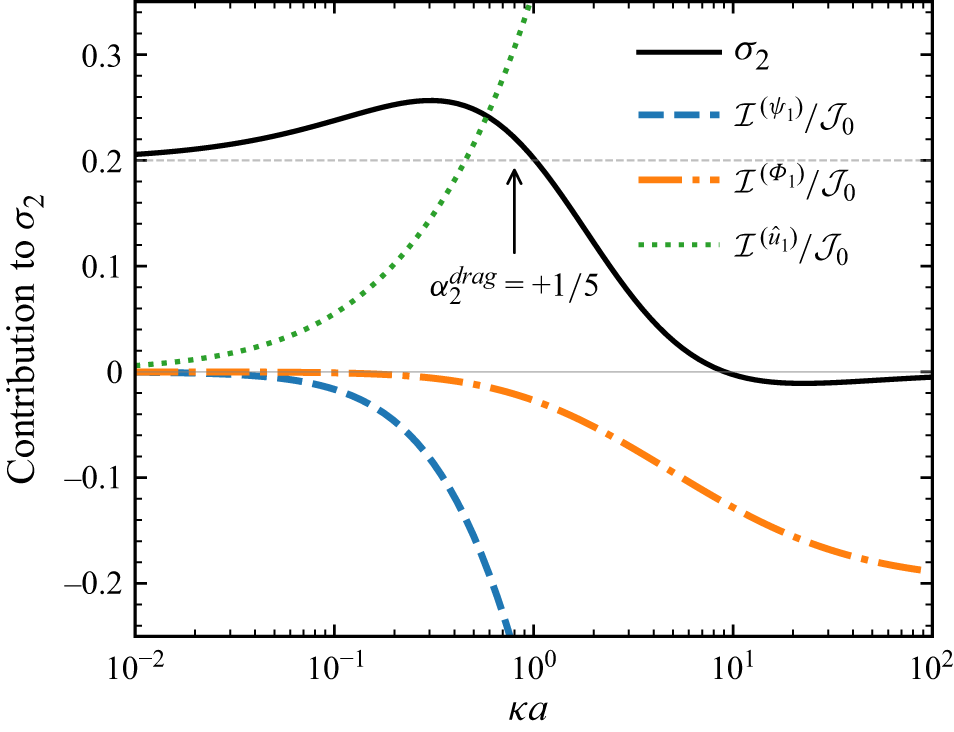
 σ2(κa)
 P2
 I(ψ1)/J0
 I(Φ1)/J0
 I(u^1)/J0
 α2drag=+1/5
 κa
 κa
 ψ1
 u^1
 Φ1
 σn≡0
 n⩾3

 C∥(κc)
 a
 c/a=0.8
 εc2=+1/6
 b
 c/a=0.6
 εc2=+4/9
 c
 c/a=0.8
 εc2=−2/15
 d
 c/a=0.6
 εc2=−4/15
 c/a=0.8
 c/a=0.6
 O(ε2)
 κc

 P2
 εc2
 c2=+0.2
 c2=+0.2
 c3=+0.25
 P2
 c2=−0.2
 c2=−0.2
 c3=+0.25
 C∥(κa)
 P3
 O(ε)

 z/a
 ρ/a
 u^0
 O(ε)
 εu^1
 u^0
 εc2=+0.2
 εc2=−0.2
 P3
 c3=+0.25
 κa


 O(ε)
 f(θ)=c2P2+c3P3
 z/a
 ρ/a
 εc2=+0.15
 εc2=−0.15
 εc2=+0.10
 εc3=+0.10
 εc2=−0.10
 εc3=+0.15
 r=a[1+εf(θ)]
 εψ1/ζ
 κa=2
 εΦ1/(E∞a)
 n=3
 εu^1/U^
 Φ1
 u^1
 κa
 ψ1
 κa
 κa=2
 cn


 Open access

