2.1 Data and Quantities of Interest

We begin with the EI “accounting identity” (i.e., true by definition) for precinct $i$ ( $i=1,\ldots ,p$ ):

(1) $$\begin{eqnarray}T_{i}=X_{i}\unicode[STIX]{x1D6FD}_{i}^{b}+(1-X_{i})\unicode[STIX]{x1D6FD}_{i}^{w}.\end{eqnarray}$$

Following our running example, $T_{i}$ is the proportion of people in precinct $i$ turning out to vote, $X_{i}$ is the proportion of people in the precinct who are “black” (defined as nonwhite), $\unicode[STIX]{x1D6FD}_{i}^{b}$ is the proportion of black people who turn out to vote, and $\unicode[STIX]{x1D6FD}_{i}^{w}$ is the proportion of white people who turn out to vote.

Although we would like to know $\unicode[STIX]{x1D6FD}_{i}^{b}$ and $\unicode[STIX]{x1D6FD}_{i}^{w}$ for every precinct $i=1,\ldots ,p$ , the quantities of interest for this paper will be limited to the district-level proportion of blacks and whites who vote, respectively:

(2) $$\begin{eqnarray}B\equiv \mathop{\sum }_{i=1}^{p}N_{i}X_{i}\unicode[STIX]{x1D6FD}_{i}^{b}\bigg/\mathop{\sum }_{i=1}^{p}N_{i}X_{i}\quad W\equiv \mathop{\sum }_{i=1}^{p}N_{i}(1-X_{i})\unicode[STIX]{x1D6FD}_{i}^{w}\bigg/\mathop{\sum }_{i=1}^{p}N_{i}(1-X_{i}),\end{eqnarray}$$

where $N_{i}$ is the total number of people in precinct $i$ .

These quantities are related to each other, after conditioning on $T_{i}$ , by the accounting identity at the district level:

$$\begin{eqnarray}W\mathop{\sum }_{i=1}^{p}N_{i}(1-X_{i})+B\mathop{\sum }_{i=1}^{p}N_{i}X_{i}=\mathop{\sum }_{i=1}^{p}N_{i}T_{i},\end{eqnarray}$$

so one can be derived from the other. Therefore, we focus only on the inference about $B$ from here on.

2.2 The (Nonidentified) Model

We now allow “contextual effects”, which in this example means that the race-specific turnout proportions ( $\unicode[STIX]{x1D6FD}_{i}^{b}$ and $\unicode[STIX]{x1D6FD}_{i}^{w}$ ) are allowed to depend on the “context” (e.g., the black proportion $X_{i}$ ). The only essential assumption we make in this paper is as follows:

Assumption 1 (Linear contextual effects).

The random vector $(\unicode[STIX]{x1D6FD}_{i}^{b},\unicode[STIX]{x1D6FD}_{i}^{w},X_{i},N_{i})$ is independent and identically distributed over $i$ , for $i=1,\ldots ,p$ , and satisfies

(3) $$\begin{eqnarray}E(\unicode[STIX]{x1D6FD}_{i}^{w}|X_{i},N_{i})=w_{0}+w_{1}X_{i}\end{eqnarray}$$

and

(4) $$\begin{eqnarray}E(\unicode[STIX]{x1D6FD}_{i}^{b}|X_{i},N_{i})=b_{0}+b_{1}X_{i},\end{eqnarray}$$

where $w_{0},w_{1},b_{0},b_{1}$ are nonrandom real parameters.

The current form of the assumption implies that $E(\unicode[STIX]{x1D6FD}_{i}^{b,w}|X_{i},N_{i})=E(\unicode[STIX]{x1D6FD}_{i}^{b,w}|X_{i})$ (where $\unicode[STIX]{x1D6FD}_{i}^{b,w}$ means that this expression holds for $\unicode[STIX]{x1D6FD}_{i}^{b}$ and also $\unicode[STIX]{x1D6FD}_{i}^{w}$ ), and, therefore, $N_{i}$ can be omitted. Supplementary Appendix C explains how the effect of $N_{i}$ can be included in the regression. In the main text, however, we adopt this simpler form of the model omitting $N_{i}$ since this retains the essential feature of partial identification and it is more common in the literature (see, e.g., Achen and Shively Reference Achen and Shively1995; King Reference King1997, Section 3.2; Altman, Gill, and McDonald Reference Altman, Gill, McDonald, King, Rosen and Tanner2004).

Under these assumptions, $(\unicode[STIX]{x1D6FD}_{i}^{b},\unicode[STIX]{x1D6FD}_{i}^{w},X_{i})$ from each precinct is a vector of random variables sampled from an underlying probability distribution. The conditional expectations $E(\unicode[STIX]{x1D6FD}_{i}^{b,w}|X_{i})$ are taken over the conditional distribution of $\unicode[STIX]{x1D6FD}_{i}^{b,w}$ , given $X_{i}$ , which allows for $\unicode[STIX]{x1D6FD}_{i}^{b,w}$ to still be random even after fixing the values of $X_{i}$ . For example, precincts with similar $X_{i}$ ’s (e.g., around 0.5) can still have very different race-specific voting proportions, $\unicode[STIX]{x1D6FD}_{i}^{b}$ or $\unicode[STIX]{x1D6FD}_{i}^{w}$ .

Under the assumptions regarding $E(\unicode[STIX]{x1D6FD}_{i}^{b,w}|X_{i})$ , the accounting identity (1) now implies a quadratic regression:

(5) $$\begin{eqnarray}\displaystyle E(T_{i}|X_{i}) & = & \displaystyle w_{0}+(b_{0}-w_{0}+w_{1})X_{i}+(b_{1}-w_{1})X_{i}^{2}\end{eqnarray}$$

(6) $$\begin{eqnarray}\displaystyle & = & \displaystyle w_{0}+c_{1}X_{i}+d_{1}X_{i}^{2},\end{eqnarray}$$

where

(7) $$\begin{eqnarray}c_{1}=b_{0}-w_{0}+w_{1}\quad \text{and}\quad d_{1}=b_{1}-w_{1}\end{eqnarray}$$

are the coefficients of $X_{i}$ and $X_{i}^{2}$ , respectively. It then follows that the three parameters $(w_{0},c_{1},d_{1})$ are identifiable (if the $X_{i}$ ’s can take three or more distinct values) and can be estimated by (possibly weighted) least squares regression.

The four regression parameters in the linear contextual effects model are related to the three regression parameters in the quadratic regression of $T_{i}$ vs $X_{i}$ via

(8) $$\begin{eqnarray}(w_{0},w_{1},b_{0},b_{1})=(w_{0},w_{1},c_{1}+w_{0}-w_{1},d_{1}+w_{1}),\end{eqnarray}$$

which are partially identifiable up to one free parameter: $(w_{0},c_{1},d_{1})$ are identified, but $w_{1}$ is not.Footnote ¹

2.3 A Simple Example

The nonidentifiability of this model described here is well-known, for example, when $b_{1}=w_{1}$ , and the resulting $T_{i}$ , $X_{i}$ relation is linear (see Freedman et al. Reference Freedman, Klein, Sacks, Smyth and Everett1991; King Reference King1997, Section 3.2).

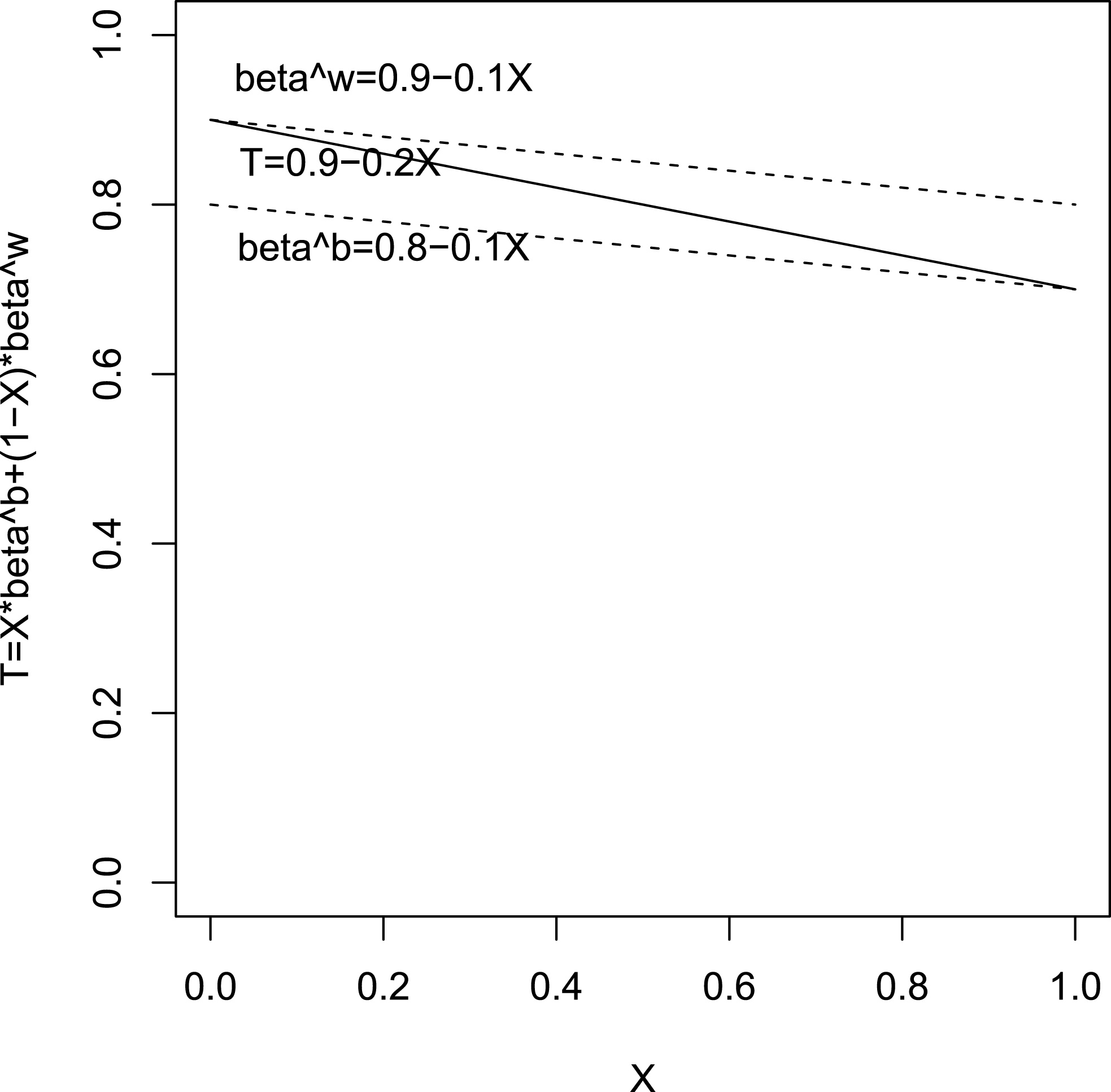
Figure 1 offers a slightly different example to illustrate the nonidentification problem, which we also use in several places below (see Sections 3.1 and 6.1.1). In this example, we observe voter turnout $T_{i}$ declining linearly as the black percentage of the precinct, $X_{i}$ , increases (see the solid black line). However, the reason for this relationship here is not necessarily determined solely from these two marginal variables. It could be that individual black citizens have lower voter turnout than white citizens and so the increasing percentage of black citizens leads to overall turnout declines. Alternatively, it could instead be that the white citizens who live in precincts with many black citizens tend to vote less, for cultural or economic reasons. In the figure, we convey the “contextual dependence” that would not normally be observable, which is how $\unicode[STIX]{x1D6FD}_{i}^{w}$ and $\unicode[STIX]{x1D6FD}_{i}^{b}$ vary over precincts; in this case, both declining as $X$ increases. This context may reflect a situation in which precincts with more black citizens happen to be from poorer, inner city areas (as a result, for example, of structural discrimination), with more residential mobility and hence lower turnout.

Figure 1.

A simple example of nonidentification. The solid line is the total observed voter turnout $T_{i}$ . The underlying race-specific proportions $\unicode[STIX]{x1D6FD}_{i}^{b,w}$ can either both follow the same solid line $0.9-0.2x$ (with slope $w_{1}=-0.2$ ) or separately follow the two dashed lines $0.9-0.1x$ and $0.8-0.1x$ (with slope $w_{1}=-0.1$ ). The slope parameter $w_{1}$ (for $\unicode[STIX]{x1D6FD}_{i}^{w}$ ) is therefore not identified. (Another possible value $w_{1}=0$ corresponds to a scenario of constant $(\unicode[STIX]{x1D6FD}_{i}^{b},\unicode[STIX]{x1D6FD}_{i}^{w})=(0.7,0.9)$ .)

2.4 Conflicting Advice on Identifying Assumptions

The key problem, then, is that the linear contextual effects model has four parameters, but the derived quadratic regression of the observed $T_{i}$ versus $X_{i}$ can only identify three of them. Existing works have addressed this issue, providing at times conflicting advice. In particular, scholars have suggested treating the nonidentified parameter $w_{1}$ by setting $w_{1}=\max \{-d_{1},0\}$ (Achen and Shively Reference Achen and Shively1995; Altman, Gill, and McDonald Reference Altman, Gill, McDonald, King, Rosen and Tanner2004), $w_{1}=0$ (Wakefield Reference Wakefield, King, Rosen and Tanner2004, Section 1.2), and $w_{1}=-d_{1}/2$ (Wakefield Reference Wakefield, King, Rosen and Tanner2004, Section 1.2). Of course, the advice in each case is given with warnings and is appropriate in some circumstances but are neither universally appropriate nor come with decision rules to help researchers decide when to use each one. Ultimately, each of these assumptions is arbitrary, meaning that the results using it give answers that are highly model dependent. In real applications, these assumptions can make a major substantive difference in empirical results.

The approach we introduce below differs in an important respect from this literature. Instead of arbitrarily picking a value for $w_{1}$ and hoping it applies across datasets or to the one before us, we derive a prior-insensitive bound for $w_{1}$ under the current linear contextual effects model, using the expectations of the DD bounds conditional on the $X_{i}$ ’s. Our approach is conditional on the linearity of the contextual effects model but should be relatively robust to many types of deviations from linearity.

3.1 Intuition

Denote the DD bounds for the unobserved $\unicode[STIX]{x1D6FD}_{i}^{w}$ as $L_{i}\leqslant \unicode[STIX]{x1D6FD}_{i}^{w}\leqslant U_{i}$ , where $L_{i}\equiv \max \{0,(T_{i}-X_{i})/(1-X_{i})\}$ and $U_{i}\equiv \min \{1,T_{i}/(1-X_{i})\}$ . Under the linear contextual model $E(\unicode[STIX]{x1D6FD}_{i}^{w}|X_{i})=w_{0}+w_{1}X_{i}$ , the observable DD bounds $L_{i}\leqslant \unicode[STIX]{x1D6FD}_{i}^{w}\leqslant U_{i}$ form a problem of interval data regression, regressing $[L_{i},U_{i}]$ against $X_{i}$ . It is well-known (see, e.g., Chernozhukov, Hong, and Tamer Reference Chernozhukov, Hong and Tamer2007; Liao and Jiang Reference Liao and Jiang2010) that although interval data regression cannot fully identify the regression coefficients, it can provide their identification regions or bounds. We use this perspective to derive a bound for the nonidentified regression coefficient $w_{1}$ .

Taking expectations under the linear contextual model gives the corresponding bound in the conditional expectation, $E(L_{i}|X_{i})\leqslant E(\unicode[STIX]{x1D6FD}_{i}^{w}|X_{i})\leqslant E(U_{i}|X_{i})$ , or

(9) $$\begin{eqnarray}E(L_{i}|X_{i})\leqslant w_{0}+w_{1}X_{i}\leqslant E(U_{i}|X_{i}).\end{eqnarray}$$

These bounds are identifiable from observable quantities. Forcing this bound in the entire domain of $X_{i}$ leads to a bound for $w_{1}$ .

Figure 2.

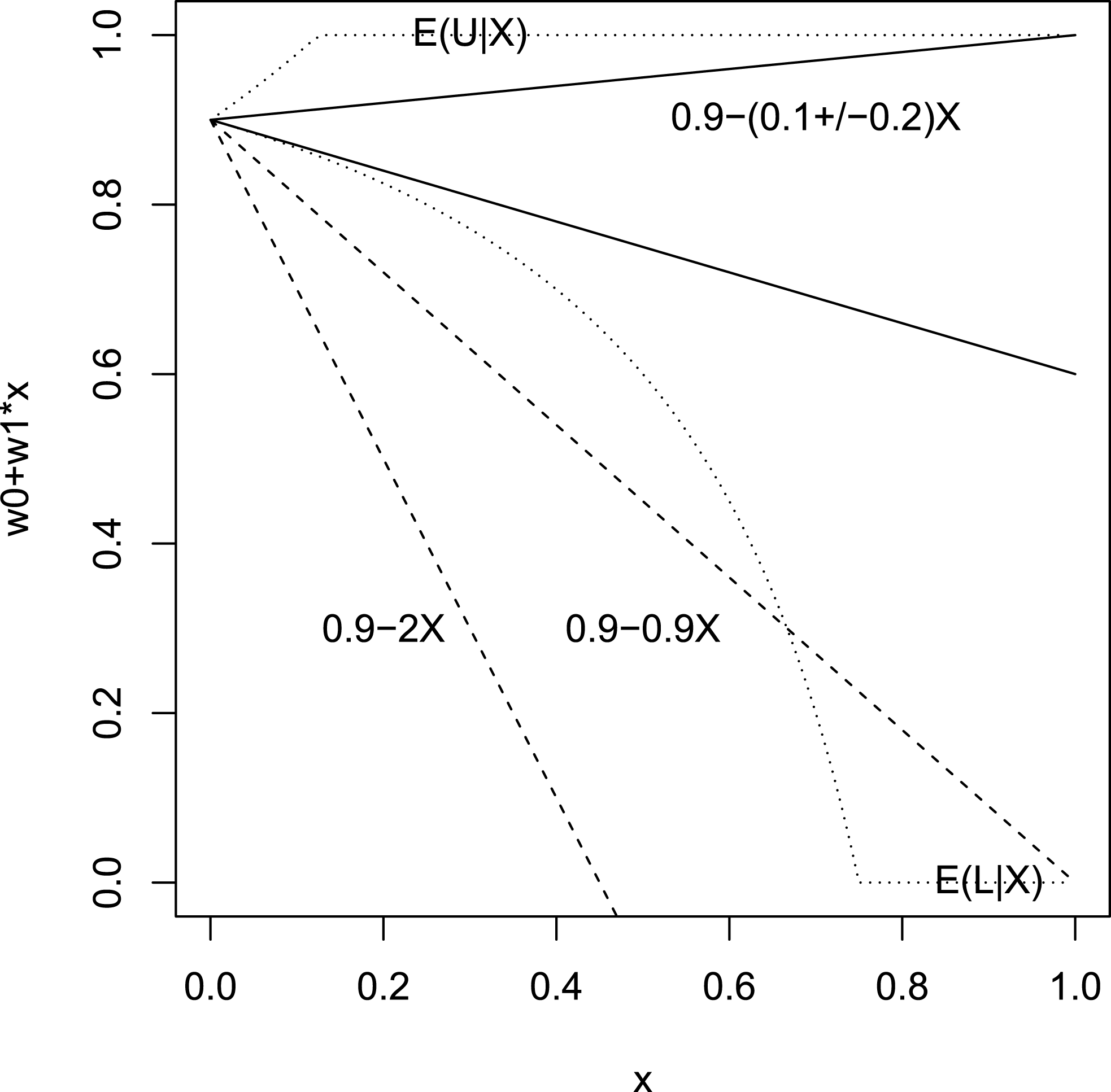
Intuition for bounding $w_{1}$ . The dotted curves are the expectations of the DD bounds for $\unicode[STIX]{x1D6FD}_{i}^{w}$ for the simple example of Section 2.3. The solid lines $0.9-(0.1\pm 0.2)x$ are obtained by forcing linear contextual effects $E(\unicode[STIX]{x1D6FD}_{i}^{w}|X_{i}=x)=w_{0}+w_{1}x$ to lie between the dotted curves. The dashed lines are examples exceeding the expectation of the DD upper bound (see Section 3.1).

Consider the simple example from Section 2.3, where $T_{i}=0.9-0.2X_{i}$ .

In Figure 2, we illustrate the intuition of how to bound the slope parameter $w_{1}$ in the linear contextual model $E(\unicode[STIX]{x1D6FD}_{i}^{w}|X_{i}=x)=w_{0}+w_{1}x$ for all $x\in (0,1)$ . The intercept parameter is identifiable as $w_{0}=E(T_{i}|X_{i}=0)=0.9$ . The slope parameter $w_{1}$ is nonidentified, but only partially so. There are hidden constraints: if the line $w_{0}+w_{1}x=0.9-2x$ , then the probability $E(\unicode[STIX]{x1D6FD}_{i}^{w}|X_{i}=x)=w_{0}+w_{1}x$ can be negative; so $w_{1}$ cannot be as low as $-2$ ( $w_{1}\geqslant -2$ ). Even if we choose $w_{0}+w_{1}x=0.9-0.9x$ so that $E(\unicode[STIX]{x1D6FD}^{w}|X_{i}=x)=w_{0}+w_{1}x$ falls between $[0,1]$ for all $x\in (0,1)$ , the line $0.9-0.9x$ can still penetrate a large portion of the dotted curve of the expectation of the DD lower bound $E(L_{i}|X_{i}=x)$ . As such, $w_{1}$ also cannot be as low as $-0.9$ ( $w_{1}\geqslant -0.9$ ). In fact, to force $w_{0}+w_{1}x$ to fall between the dotted curves $[E(L_{i}|X_{i}=x),E(U_{i}|X_{i}=x)]$ for all $x\in (0,1)$ , we need to have $w_{1}\in [-0.3,0.1]=-0.1\pm 0.2$ , restricted to a small interval in this example. (Incidentally, this bound includes all the three possibilities $w_{1}=-0.2$ , $w_{1}=-0.1$ , and $w_{1}=0$ , as described in the original example in Figure 1.)

Intuitively, this is how we exploit the expectation of the DD bound (9) to bound the nonidentified contextual effect parameter $w_{1}$ . More formally, we have the following theoretical results.

3.2 Theory

The following proposition provides a necessary and sufficient condition for this bound in terms of the only nonidentified parameter $w_{1}$ .

Proposition 1. Assume a linear contextual effect $E(\unicode[STIX]{x1D6FD}_{i}^{w}|X_{i})=w_{0}+w_{1}X_{i}$ for all $X_{i}\in A$ where $A\subset (0,1)$ . Then

$$\begin{eqnarray}E(L_{i}|X_{i})\leqslant E(\unicode[STIX]{x1D6FD}_{i}^{w}|X_{i})\leqslant E(U_{i}|X_{i}),\end{eqnarray}$$

for all $X_{i}\in A$ , if and only if the nonidentifiable parameter $w_{1}$ satisfies

$$\begin{eqnarray}\sup _{X_{i}\in A}[(E(L_{i}|X_{i})-w_{0})/X_{i}]\leqslant w_{1}\leqslant \inf _{X_{i}\in A}[(E(U_{i}|X_{i})-w_{0})/X_{i}].\end{eqnarray}$$

The above proposition then gives the tightest bound possible on $w_{1}$ . The upper bound and the lower bound are both constructed out of identifiable quantities. The functions $E(L_{i}|X_{i})$ and $E(U_{i}|X_{i})$ may be estimated by lowess smoothing. If for some reason we would like to avoid such nonparametric estimation (e.g., it may not perform well at boundary values of $X_{i}$ ), we can relax the bounds somewhat and incorporate results from a parametric regression $E(T_{i}|X_{i})=w_{0}+c_{1}X_{i}+d_{1}X_{i}^{2}$ .

Proposition 2. For all $X_{i}\in [l,u]\subset (0,1)$ where $l<u$ , assume linear contextual effect $E(\unicode[STIX]{x1D6FD}_{i}^{w}|X_{i})=w_{0}+w_{1}X_{i}$ and a quadratic regression $E[T_{i}|X_{i}]=w_{0}+c_{1}X_{i}+d_{1}X_{i}^{2}$ . Then we have

$$\begin{eqnarray}wl\leqslant w_{1}\leqslant wu,\end{eqnarray}$$

where $wl=\max _{x\in \{l,u\}}\max \{-w_{0}/x,(w_{0}+c_{1}+d_{1}-1)/(1-x)-d_{1}\}$ and $wu=\min _{x\in \{l,u\}}\min \{(1-w_{0})/x,(w_{0}+c_{1}+d_{1})/(1-x)-d_{1}\}$ .

Before we prove this proposition, we give some intuition on why the proposed bounds make sense. The bounds are obtained by forcing $w_{0}+w_{1}x$ and $b_{0}+b_{1}x$ (for all $x\in [l,u]$ ) to be within $[0,1]$ since these linear combinations model the $[0,1]$ -valued probabilities (via $E(\unicode[STIX]{x1D6FD}^{w,b}|X=x)$ ). For example, one of the proposed lower bounds of $w_{1}$ is of the form $-w_{0}/x$ ; this makes $w_{1}\geqslant -w_{0}/x$ and therefore $w_{0}+w_{1}x\geqslant 0$ . One of the upper bounds of $w_{1}$ is $(1-w_{0})/x$ ; this makes $w_{1}\leqslant (1-w_{0})/x$ and therefore $w_{0}+w_{1}x\leqslant 1$ . Similarly, the other two functions in the bounds are related to the bounds of $b_{0}+b_{1}x$ by using (8). Now we prove the proposition rigorously.

Proof. For the bounds in Proposition 1, note that $E(U_{i}|X_{i})=E[\min \{1,T_{i}/(1-X_{i})\}|X_{i}]\leqslant \min \{1,E[T_{i}|X_{i}]/(1-X_{i})\}$ due to Jensen’s inequality, and similarly $E(L_{i}|X_{i})\geqslant \max \{0,(E[T_{i}|X_{i}]-X_{i})/(1-X_{i})\}$ . Now apply a quadratic regression $E[T_{i}|X_{i}]=w_{0}+c_{1}X_{i}+d_{1}X_{i}^{2}$ . Then from Proposition 1, we have

$$\begin{eqnarray}\displaystyle & & \displaystyle \sup _{X_{i}\in A}\max \{-w_{0}/X_{i},(w_{0}+c_{1}-1+d_{1}X_{i})/(1-X_{i})\}\nonumber\\ \displaystyle & & \displaystyle \quad \leqslant w_{1}\leqslant \inf _{X_{i}\in A}\min \{(1-w_{0})/X_{i},(w_{0}+c_{1}+d_{1}X_{i})/(1-X_{i})\}.\nonumber\end{eqnarray}$$

Simplifying these bounds for $A=[l,u]$ with the boundary points leads to the proof.◻

To use Proposition 2, we need to supply the interval $[l,u]$ where we believe the assumptions hold. One could simply use the data range $l=\min X_{i}$ and $u=\max X_{i}$ of the dataset. However, there may be reasons to either reduce this range (e.g., if there are outliers) or increase this range (if there is a belief that the pattern could be reliably extrapolated to some extent beyond the data range). If we attempt to check the assumptions when there is no knowledge regarding the ground truth $\unicode[STIX]{x1D6FD}_{i}^{w}$ , we could still use the $(T_{i},X_{i})$ data to fit a quadratic curve on $(0,1)$ and superimpose it on the scatterplot, using it to rule out unreasonable choices of a range $[l,u]$ . For example, when quadratic regression is based on a scatterplot limited in a small domain of $X_{i}\in [0.5,0.6]$ and extrapolating the fitted quadratic curve to $x\in [0.1,0.9]$ leads to $E(T|X=x)=w_{0}+c_{1}x+d_{1}x^{2}$ breaking the “ceiling” of 1 or the “floor” of 0, then it is obvious that the range $[l,u]=[0.1,0.9]$ is too wide.

On the other hand, the bigger the set $A=[l,u]$ is for $X_{i}$ , the tighter the bounds will be in these propositions. Suppose we consider a special case $A\rightarrow (0,1)$ . In other words, we assume that the previous quadratic regression model holds for all $X_{i}$ in the whole range of $(0,1)$ . Then relaxing the bounds of Proposition 2 and taking $l\rightarrow 0$ , $u\rightarrow 1$ , we immediately have the following:

Proposition 3. For all $X_{i}\in (0,1)$ , assume linear contextual effect $E(\unicode[STIX]{x1D6FD}_{i}^{w}|X_{i})=w_{0}+w_{1}X_{i}$ and a quadratic regression $E[T_{i}|X_{i}]=w_{0}+c_{1}X_{i}+d_{1}X_{i}^{2}$ . Then we have

$$\begin{eqnarray}wl\leqslant w_{1}\leqslant wu,\end{eqnarray}$$

where $wl=\max \{-w_{0},c_{1}+w_{0}-1\}$ and $wu=\min \{1-w_{0},c_{1}+w_{0}\}$ .

4.1 Estimating District-Level Parameters

We first analyze the precinct-level parameter $\unicode[STIX]{x1D6FD}_{i}^{b}$ . Denote residuals as $e_{i}^{b}=\unicode[STIX]{x1D6FD}_{i}^{b}-E(\unicode[STIX]{x1D6FD}_{i}^{b}|X_{i})$ , $e_{i}^{w}=\unicode[STIX]{x1D6FD}_{i}^{w}-E(\unicode[STIX]{x1D6FD}_{i}^{w}|X_{i})$ . Note that

(10) $$\begin{eqnarray}\displaystyle \unicode[STIX]{x1D6FD}_{i}^{b} & = & \displaystyle E(\unicode[STIX]{x1D6FD}_{i}^{b}|X_{i})+e_{i}^{b}\end{eqnarray}$$

(11) $$\begin{eqnarray}\displaystyle & \stackrel{\text{by (8)}}{=} & \displaystyle w_{0}+(c_{1}-w_{1})+(w_{1}+d_{1})X_{i}+e_{i}^{b}\end{eqnarray}$$

(12) $$\begin{eqnarray}\displaystyle & = & \displaystyle [w_{0}+c_{1}+d_{1}X_{i}]+w_{1}(X_{i}-1)+e_{i}^{b}\end{eqnarray}$$

(13) $$\begin{eqnarray}\displaystyle & \equiv & \displaystyle b_{i}(w_{1},\unicode[STIX]{x1D703})+e_{i}^{b},\end{eqnarray}$$

where $\unicode[STIX]{x1D703}\equiv (w_{0},c_{1},d_{1})^{T}$ .

The district-level parameter is given as

(14) $$\begin{eqnarray}\displaystyle B & \equiv & \displaystyle \mathop{\sum }_{i=1}^{p}N_{i}X_{i}\unicode[STIX]{x1D6FD}_{i}^{b}/\mathop{\sum }_{i=1}^{p}N_{i}X_{i}\end{eqnarray}$$

(15) $$\begin{eqnarray}\displaystyle & = & \displaystyle \frac{\mathop{\sum }_{i=1}^{p}N_{i}X_{i}b_{i}(w_{1},\unicode[STIX]{x1D703})}{\mathop{\sum }_{i=1}^{p}N_{i}X_{i}}+\frac{\mathop{\sum }_{i=1}^{p}N_{i}X_{i}e_{i}^{b}}{\mathop{\sum }_{i=1}^{p}N_{i}X_{i}}.\end{eqnarray}$$

By the Law of Large Numbers, for large $p$ , we can ignore the second term of the expansion of (14) with the mean zero residuals $e_{i}^{b}$ , when estimating $B$ . We can then form a point estimate of $B$ using the first term:

(16) $$\begin{eqnarray}\displaystyle B(w_{1},\unicode[STIX]{x1D703}) & \equiv & \displaystyle \frac{\mathop{\sum }_{i=1}^{p}N_{i}X_{i}b_{i}(w_{1},\unicode[STIX]{x1D703})}{\mathop{\sum }_{i=1}^{p}N_{i}X_{i}}\nonumber\\ \displaystyle & = & \displaystyle \frac{\mathop{\sum }_{i=1}^{p}N_{i}X_{i}b_{i}(0,\unicode[STIX]{x1D703})}{\mathop{\sum }_{i=1}^{p}N_{i}X_{i}}-w_{1}\frac{\mathop{\sum }_{i=1}^{p}N_{i}X_{i}(1-X_{i})}{\mathop{\sum }_{i=1}^{p}N_{i}X_{i}},\end{eqnarray}$$

where

(17) $$\begin{eqnarray}b_{i}(w_{1},\unicode[STIX]{x1D703})\equiv [w_{0}+c_{1}+d_{1}X_{i}]+w_{1}(X_{i}-1).\end{eqnarray}$$

4.2 Sensitivity of District Cell Value Estimate

The point estimate $B(w_{1},\unicode[STIX]{x1D703})$ will vary with $w_{1}$ due to (16). The sensitivity on $w_{1}$ can be measured by

(18) $$\begin{eqnarray}\frac{\unicode[STIX]{x2202}B(w_{1},\unicode[STIX]{x1D703})}{\unicode[STIX]{x2202}w_{1}}=-r\equiv -\frac{\mathop{\sum }_{i=1}^{p}N_{i}X_{i}(1-X_{i})}{\mathop{\sum }_{i=1}^{p}N_{i}X_{i}},\end{eqnarray}$$

which is typically nonzero (unless $X_{i}\in \{0,1\}$ for all nonempty precincts). Therefore, the bounds we derived earlier for $w_{1}$ will be very useful here for limiting the scope of the influence by $w_{1}$ .

For any possible value of the partially identified $w_{1}$ , the district-level parameter $B=\sum _{i}N_{i}X_{i}\unicode[STIX]{x1D6FD}_{i}^{b}/\sum _{i}N_{i}X_{i}$ is estimated by the point estimator $B(w_{1},\unicode[STIX]{x1D703})$ following (16). We will now use the bounds on $w_{1}$ to bound this district-level parameter estimate $B(w_{1},\unicode[STIX]{x1D703})$ , and estimate its $\unicode[STIX]{x1D703}$ parameter by regression.

4.3 Bounding District Cell Value

Due to Proposition 2 or Proposition 3, we know that $w_{1}\in [wl,wu]$ , where $wu=wu(\unicode[STIX]{x1D703})$ and $wl=wl(\unicode[STIX]{x1D703})$ depend on $\unicode[STIX]{x1D703}$ . Then

(19) $$\begin{eqnarray}B(w_{1},\unicode[STIX]{x1D703})\in [Bl,Bu]\equiv [B(wu(\unicode[STIX]{x1D703}),\unicode[STIX]{x1D703}),B(wl(\unicode[STIX]{x1D703}),\unicode[STIX]{x1D703})].\end{eqnarray}$$

The parameters $\unicode[STIX]{x1D703}=(w_{0},c_{1},d_{1})^{T}$ can be estimated from a least squares regression

(20) $$\begin{eqnarray}\hat{\unicode[STIX]{x1D703}}=({\hat{w}}_{0},{\hat{c}}_{1},\hat{d}_{1})^{T}\leftarrow \min _{w_{0},c_{1},d_{1}}\frac{\mathop{\sum }_{i=1}^{p}\unicode[STIX]{x1D70C}_{i}[T_{i}-(w_{0}+c_{1}X_{i}+d_{1}X_{i}^{2})]^{2}}{\mathop{\sum }_{i=1}^{p}\unicode[STIX]{x1D70C}_{i}},\end{eqnarray}$$

possibly weighted by some choice $\unicode[STIX]{x1D70C}_{i}$ .

Replacing $\unicode[STIX]{x1D703}$ in (19) by $\hat{\unicode[STIX]{x1D703}}$ , we obtain the estimated bounds for the district parameter $B$ . Since this is implied from a regression model of linear contextual effects, one may call this a ‘‘regression bound,” which will be our proposed interval estimate for $B$ .

Definition 1 (Regression bound).

Footnote ² A regression bound for the district parameter $B=\sum _{i}N_{i}X_{i}\unicode[STIX]{x1D6FD}_{i}^{b}/\sum _{i}N_{i}X_{i}$ is of the form

(21) $$\begin{eqnarray}[\hat{B}l,\hat{B}u]\equiv [B(wu(\hat{\unicode[STIX]{x1D703}}),\hat{\unicode[STIX]{x1D703}}),B(wl(\hat{\unicode[STIX]{x1D703}}),\hat{\unicode[STIX]{x1D703}})],\end{eqnarray}$$

where the functional form of the point estimate $B(w_{1},\unicode[STIX]{x1D703})$ follows (16), $wu=wu(\unicode[STIX]{x1D703})$ and $wl=wl(\unicode[STIX]{x1D703})$ are the bounds of the $w_{1}$ parameter according to Proposition 2 or Proposition 3, and $\hat{\unicode[STIX]{x1D703}}$ estimates the regression coefficients $\unicode[STIX]{x1D703}$ from (20).

6.1 Theoretical

We will compare the proposed bound $\text{CI}_{x}$ to the Duncan and Davis (Reference Duncan and Davis1953) bound DD, as defined in Proposition 4. For any interval $A$ , we will use $|A|$ to denote its length. We will use $x=0$ and $x=1$ for illustration.

To measure the success of the proposed method, we examine:

1. (1) Whether the new interval estimate contains the true district parameter: $B\in \text{CI}_{x}$ .

2. (2) How narrow the new interval estimate is compared to the DD bound: the width ratio $\text{WR}_{x}\equiv |\text{CI}_{x}|/|\text{DD}|$ .

In the examples below, we assume $X\sim \text{Unif}[0,1]$ and $N_{i}$ is constant for all $i$ , unless otherwise stated.

6.1.2 Additional Examples

Example 1. $\unicode[STIX]{x1D6FD}_{i}^{b}=T+\unicode[STIX]{x1D70F}(1-X_{i})\in [0,1]$ and $\unicode[STIX]{x1D6FD}_{i}^{w}=T-\unicode[STIX]{x1D70F}X_{i}\in [0,1]$ , where probability constraints entail $\unicode[STIX]{x1D70F}\in \pm \min (T,1-T)$ and $T\in (0,1)$ . Then the plot $T_{i}$ against $X_{i}$ is a flat $T_{i}=T$ . Here, one can show by Proposition 3 that $[wl,wu]=\pm \min (T,1-T)$ . In this case, in the limit of large precincts and large number of precincts (large $N_{i}$ and $p$ ), it can be shown analytically that the true parameter $B\approx E\unicode[STIX]{x1D6FD}_{i}^{b}=T+\unicode[STIX]{x1D70F}/3\in \text{CI}_{0}\approx T\pm (1/3)\min (T,1-T)\subset \text{DD}\approx [T^{2},2T-T^{2}]$ . Also, $\text{WR}_{0}\equiv |\text{CI}_{0}|/|\text{DD}|\approx 1/[3\max (T,1-T)]\in (1/3,2/3)$ . In summary, the proposed bound tightens the DD bound while still containing the true parameter.

Example 2. $\unicode[STIX]{x1D6FD}_{i}^{b}=\unicode[STIX]{x1D70F}(1-X_{i})$ , $\unicode[STIX]{x1D6FD}_{i}^{w}=1-\unicode[STIX]{x1D70F}X_{i}$ , where $\unicode[STIX]{x1D70F}\in [0,1]$ . Then the plot $T_{i}$ against $X_{i}$ is $T_{i}=1-X_{i}$ . Here, one can show by Proposition 3 that $[wl,wu]=[-1,0]$ . In this case, in the limit of large precincts and large number of precincts (large $N_{i}$ and $p$ ), it can be shown analytically that $B\approx E\unicode[STIX]{x1D6FD}_{i}^{b}=\unicode[STIX]{x1D70F}/3\in \text{CI}_{0}\approx [0,1/3]$ , $\text{DD}\approx [0,1/2]$ . Also, $\text{WR}_{0}\equiv |\text{CI}_{0}|/|\text{DD}|\approx 2/3$ . In summary, the proposed bound tightens the DD bound while still containing the true parameter.

Example 3. $\unicode[STIX]{x1D6FD}_{i}^{b}=0$ , $\unicode[STIX]{x1D6FD}_{i}^{w}=1-X_{i}$ . Then the plot $T_{i}$ against $X_{i}$ is $T_{i}=(1-X_{i})^{2}$ . Here, one can show by Proposition 3 that $[wl,wu]=[-1,-1]$ ; so $w_{1}$ is identified. In this case, in the limit of large precincts and a large number of precincts (large $N_{i}$ and $p$ ), it can be shown analytically that $B=0$ , $\text{CI}_{0}\approx [0,0]$ , $\text{DD}\approx [0,2E\min (X,(1-X)^{2})]\approx [0,0.3032767]$ . Also, $\text{WR}_{0}\equiv |\text{CI}_{0}|/|\text{DD}|\approx 0$ .

We now generate $p=1000$ precincts all with population $N_{i}=150$ for this example. For sample estimates based on this finite dataset, we obtain true $B=0$ , $\text{DD}=[0,0.301843]$ .

We apply Proposition 2 for this example with $[l,u]=[\min (X_{i}),\max (X_{i})]=[0.001473298,0.9988792]$ .

We obtain $\hat{B}l=0.000023$ and $\hat{B}u=0.000305$ which are very close to $B=0$ , but $\text{CI}_{0}=[\hat{B}l,\hat{B}u]$ excludes the true $B$ due to sampling variation. On the other hand, the proposed interval estimate narrowly misses the true $B$ due to sampling variation. The confidence interval $\text{CI}_{x}$ for $x=1$ is $([-0.018185,0.018556]\cap \text{DD})=[0,0.018556]$ , which does contain the true $B$ now and is still very narrow. (Here, intersection with the DD bound improves the lower bound to be 0.) In summary, the regression bound $\text{CI}_{0}$ can miss the true parameter due to sampling variation. However, after expanding the bound to account for the sampling variation, $\text{CI}_{1}$ does contain the true parameter $B$ and is still much narrower than the DD bound.

Example 4. Consider $p=1000$ precincts all with population $N_{i}=150$ . We let $X_{i}\sim \text{Unif}[0,0.95]$ , $\unicode[STIX]{x1D6FD}_{i}^{b}\approx (N_{i}X_{i})^{-1}\text{Bin}(N_{i}X_{i},1/(1+\exp (-b0-b1\times X_{i}-(1-X_{i})\times \unicode[STIX]{x1D716}_{i}^{b}))$ , $\unicode[STIX]{x1D6FD}_{i}^{w}\approx (N_{i}(1-X_{i}))^{-1}\text{Bin}(N_{i}(1-X_{i}),1/(1+\exp (-w0-w1\times X_{i}-(1-X_{i})\unicode[STIX]{x1D716}_{i}^{w}))$ (the approximation ${\approx}$ here involves operations such as rounding $N_{i}X_{i}$ and adding 1 to avoid zero or fractional counts), where $\unicode[STIX]{x1D716}_{i}^{b,w}$ ’s are $\mathit{iid}$   $N(0,s^{2})$ , $s=0.5$ , $b0=2.197225$ , $b1=-1.791759$ , $w0=2.197225$ , $w1=0$ , $T_{i}\approx \unicode[STIX]{x1D6FD}_{i}^{b}X_{i}+\unicode[STIX]{x1D6FD}_{i}^{w}(1-X_{i})$ (the approximation ${\approx}$ here involves operations such as replacing $X_{i}$ by a rounded version of $N_{i}X_{i}$ divided by $N_{i}$ ). 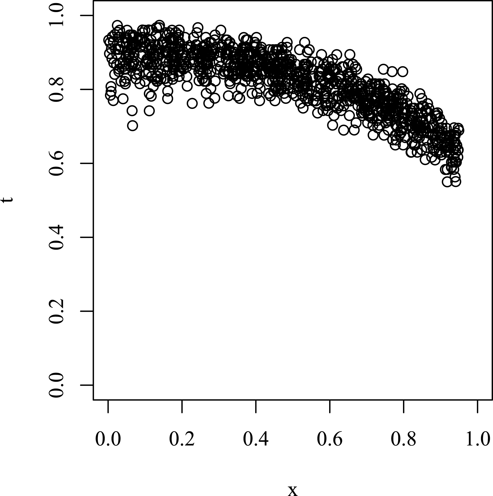The resulting $T_{i}$ versus $X_{i}$ scatterplot is given by Figure 3.

Figure 3.

$T$ versus $X$ scatterplot for Example 4.

We apply Proposition 2 for this example with $[l,u]=[\min (X_{i}),\max (X_{i})]=[0.001400,0.948935]$ .

In this case, it can be shown that $B=0.733582\in \text{CI}_{0}=[0.704450,0.750966]\subset \text{DD}=[0.636268,0.931647]$ . Also, $\text{WR}_{0}\equiv |\text{CI}_{0}|/|\text{DD}|=0.157478$ .

The $\text{CI}_{1}$ is $[0.682944,0.772162]$ , which is also narrower than the DD interval and contains the true $B$ .

Example 5. Consider $p=1000$ precincts all with population $N_{i}=150$ . We let $X_{i}\sim \text{Unif}[0,0.7]$ , $\unicode[STIX]{x1D6FD}_{i}^{b}\approx (N_{i}X_{i})^{-1}\text{Bin}(N_{i}X_{i},1/(1+\exp (-b0-b1\times X_{i}-(1-X_{i})\times \unicode[STIX]{x1D716}_{i}^{b}))$ , $\unicode[STIX]{x1D6FD}_{i}^{w}\approx (N_{i}(1-X_{i}))^{-1}\text{Bin}(N_{i}(1-X_{i}),1/(1+\exp (-w0-w1\times X_{i}-(1-X_{i})\unicode[STIX]{x1D716}_{i}^{w}))$ (the approximation ${\approx}$ here involves operations such as rounding $N_{i}X_{i}$ and adding 1 to avoid zero or fractional counts), where $\unicode[STIX]{x1D716}_{i}^{b,w}$ ’s are $\mathit{iid}$   $N(0,s^{2})$ , $s=1$ , $b0=0$ , $b1=0$ , $w0=2.197225$ , $w1=0$ , $T_{i}\approx \unicode[STIX]{x1D6FD}_{i}^{b}X_{i}+\unicode[STIX]{x1D6FD}_{i}^{w}(1-X_{i})$ (the approximation ${\approx}$ here involves operations such as replacing $X_{i}$ by a rounded version of $N_{i}X_{i}$ divided by $N_{i}$ ). 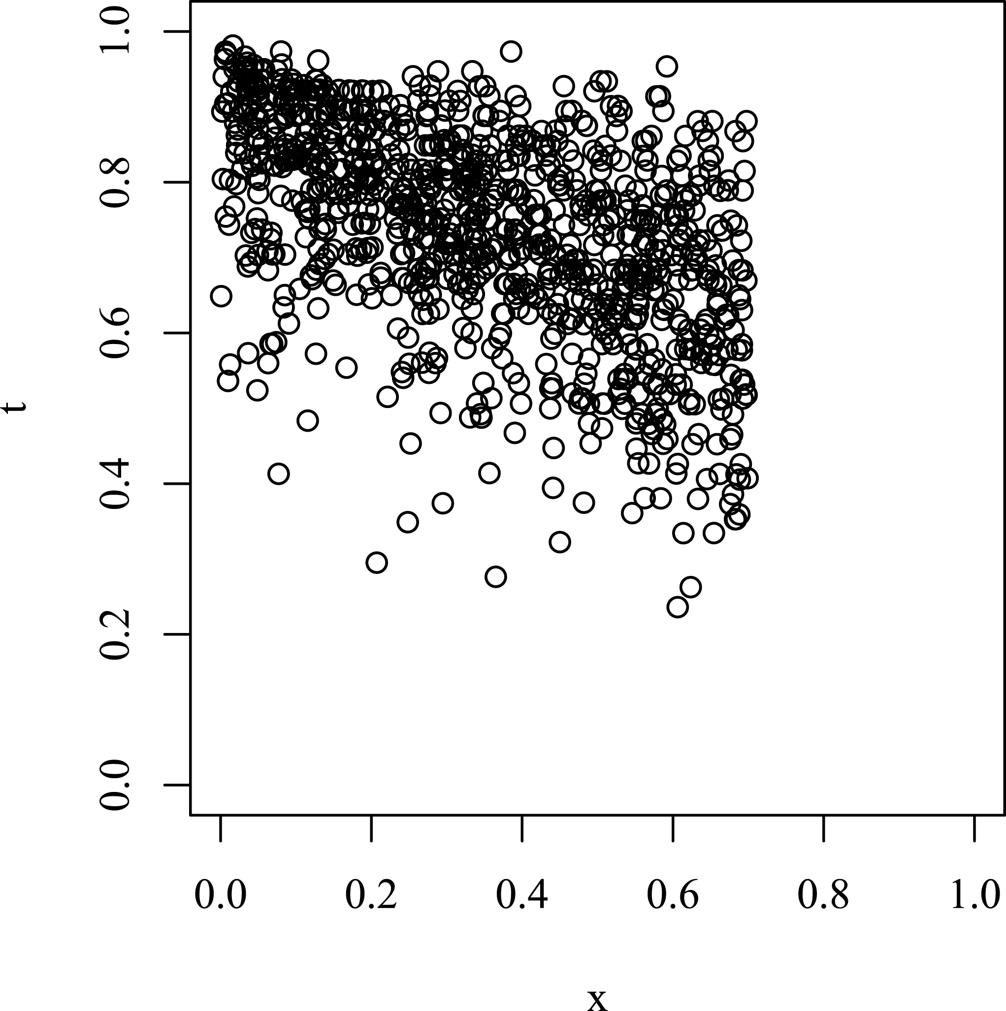The resulting $T_{i}$ versus $X_{i}$ scatterplot is given by Figure 4.

Figure 4.

$T$ versus $X$ scatterplot for Example 5.

We apply Proposition 2 for this example with $[l,u]=[\min (X_{i}),\max (X_{i})]=[0.001031,0.699215]$ .

In this case, it can be shown that $B=0.499342\in \text{CI}_{0}=[0.399895,0.759834]\subset \text{DD}=[0.340341,0.961388]$ . Also, $\text{WR}_{0}\equiv |\text{CI}_{0}|/|\text{DD}|=0.579568$ .

The $\text{CI}_{1}$ is $[0.368232,0.799369]$ , which is also narrower than the DD interval and contains the true $B$ .

The $\text{CI}_{1}$ used in Examples 3–5 will have at least $\unicode[STIX]{x1D6F7}(1)\approx 84\%$ coverage probability asymptotically, according to Proposition 4. In repetitions of 1000 simulations, we found that $\text{CI}_{1}$ is very conservative: $P[B\in \text{CI}_{1}]=944/1000,1000/1000,1000/1000$ , respectively, in Examples 3, 4, and 5. The comparison for (mean width of $\text{CI}_{1}$ , mean width of DD bound) is $(0.0178,0.3032),(0.0946,0.2974),(0.4405,0.6227)$ , respectively. These results demonstrate that the proposed confidence intervals are considerably more informative about $B$ compared to the DD bounds, as shown in repeated simulations.

It is noted that in Examples 4 and 5, the true models do not follow the linear contextual model or quadratic regression of $T_{i}$ versus $X_{i}$ . The $\unicode[STIX]{x1D6FD}_{i}^{b,w}$ ’s follow overdispersed logistic regression model with heteroscedastic normal random effects.

6.2 Empirical

Given that some information is forever lost during the process of aggregating individual-level data, it is important to develop models tuned to the specific types of datasets similar to those used in practice. Unfortunately, for the very reason that EI is a problem in the first place, datasets with true labels in target application areas, such as elections and voting rights litigation, are typically not available. The nature of the learning problem is thus intrinsically much more difficult than a traditional supervised learning problem where labeled examples sampled from the target distribution are abundant. As such, the most recent work on EI has evaluated approaches using a very small number of datasets with ground truth, combined with artificial, simulated data. Here, we dramatically increase the number of datasets with ground truth labels on social data for evaluation of our proposed model as well as to serve as a test bed for future approaches to EI model building. We describe the data we collected followed by our empirical results.

6.2.2 Analysis

Our goal is scientifically appropriate EI (including, when appropriate, conclusions such as “we don’t know anything”) even in the presence of (a) assumptions that are violated and (b) data where most or all of the relevant individual-level information has been aggregated away. The specific method we evaluate here has no adjustable parameters and works on all input data. It begins with the easy-to-apply bounds of Proposition 2 based on a quadratic regression (leaving the nonparametric regression approach in Proposition 1 to future work because it involves tuning the smoothing parameter and is harder to derive the confidence intervals). The method then uses $\text{CI}_{x}$ if $\hat{B}l\leqslant \hat{B}u$ and DD covers part of $\text{CI}_{0}$ , and otherwise reverts to the DD bounds. (This simple heuristic eliminates cases when the bounds flip, which can occur in practice when assumptions are violated; see Supplementary Appendix B, Remark 2.)

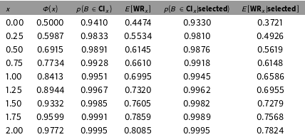
Table 1 displays the effectiveness of our methodology for all datasets in our collection, given differing confidence levels, $\unicode[STIX]{x1D6F7}(x)$ (in the second column). We observe (in the third column) that our proposed bounds consistently capture the true value more often than the nominal coverage intervals, meaning that our bounds are highly accurate but also conservative. For example, at the 96% confidence interval (second to last row), our bounds capture the truth 99.91% of the time rather than 96%. The improvement relative to DD appears as the ratio of the length of our new confidence interval to the length of the original DD bound width, as reported in the fourth column. This number is always less than 1.0, often substantially so.

Table 1.

Effectiveness in terms of the nominal coverage probability, $\unicode[STIX]{x1D6F7}(x)$ ; proportion of intervals that capture the true district value, $p(B\in \text{CI}_{x})$ ; and the width ratio among those selected. The last two columns repeat the previous two among only the 88% of the datasets that do not revert to DD bounds.

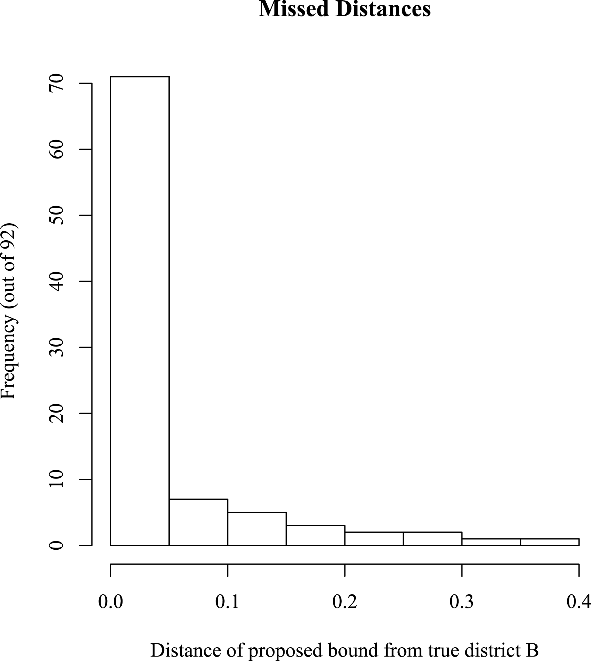
By inferring from these data, we recommend that, in practice, researchers use our bounds while setting $x=0.5$ (see the third row of numbers for $\text{CI}_{0.5}$ ), which is a reasonable trade-off between the capture probability and the width ratio for the observed datasets. It captures the truth in 98.9% of our 8,430 datasets and narrows the bounds by 38.5% relative to the 65-year-old DD bounds. We also analyze 92 of the 8,430 datasets where the bounds do not capture the truth, by constructing Figure 5. The figure gives a histogram of the size of the misses, the vast majority of which are very small, almost all less than 0.05.

Figure 5.

Histogram for how far away the true $B$ falls outside of $\text{CI}_{0.5}$ for the 92 datasets (out of the total 8,430) for which the bounds were applied, but the true district-level $B$ value was not captured.

For completeness, we also repeat the calculation for columns 3 and 4 among only those datasets where our method does not revert to DD bounds. These results appear in the final two columns. Because our method reverts to the DD bounds in only 12% of our datasets, narrowing the bounds in the remaining 88%, the last two columns do not differ much from columns 3 and 4.

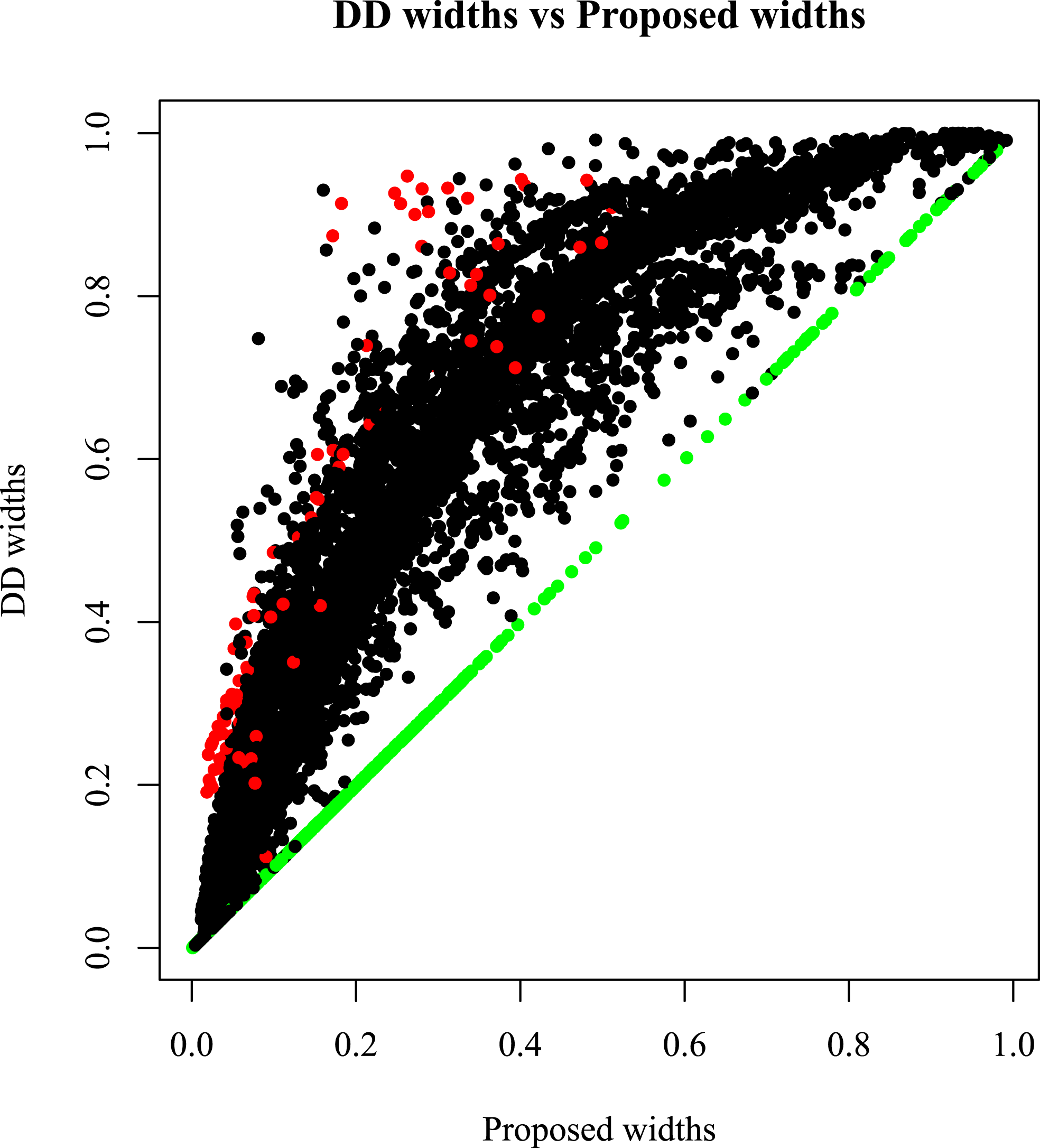
Finally, we summarize these results in Figure 6 by plotting the width of our proposed bounds (horizontally) by the width of the DD bounds (vertically). Each dot is one of our 8,430 datasets. The green dots on the diagonal represent the 12% of datasets for which our method automatically returned the DD bound. For all others, the bounds are narrower and thus more informative, which is reflected in the figure by being above the diagonal line. Among these, the few red dots are those where the truth is not captured and the mass of black dots is where the truth is captured. The figure reveals that our approach is able to improve the most over the DD bounds when the DD bounds have widths farther from the 0 or 1 extremes of the unit interval.

Figure 6.

Widths of the proposed bounds relative to the DD bounds. Green points represent datasets in which the bounds reverted to those of the DD bounds, and red points indicate the 92 datasets (out of the total 8,430) for which the bounds were applied, but the true district-level $B$ value was not captured.

Overall, the results of analyzing more than 8,000 datasets with known truth suggest that our approach generates considerably more information than the bounds proposed by, and used routinely in the literature since, Duncan and Davis (Reference Duncan and Davis1953) with very little cost.

7.1 Limitations

Our work adds a single essential assumption, requiring contextual effects, if any, to be linear (Assumption 1). This is far more general than the traditional approaches, which assume zero contextual effects (or effects that have zero correlation with $X$ ) and which are regularly falsified by real data with knowledge of the ground truth. Much of the problem with Goodman’s regression giving answers outside of the known DD bounds is precisely because of this implicit zero contextual effect assumption that we generalize and thus avoid.

Yet, when Assumption 1 fails, the bounds produced by our method may not capture the truth. The key questions in practice are how often such problems occur and how can one know about such violations. Fortunately, we have found in Section 6.2 that violations bad enough to violate our bounds are rare in our collection of datasets. However, in the difficult field of EI, we must constantly be aware that it is always theoretically possible to violate assumptions without any signal in observable data. Consider the following example:

If all datasets were generated from this model (e.g., with $b_{2}=T=1/3$ ), then the asymptotic coverage probability of any $\text{CI}_{x}$ would be 0 and we would not be able to avoid such data sets without knowledge of the ground truth. Fortunately, this kind of “nondetectable violation” happens quite rarely, at least in our data. For example, the nondetectable violation in Example 6 is caused by the quadratic effects in $\unicode[STIX]{x1D6FD}_{i}^{b}$ and $\unicode[STIX]{x1D6FD}_{i}^{w}$ canceling each other exactly by chance. In addition, our interval estimates are robust in the sense that even a small amount of violation of the assumptions do not matter. For example, the quadratic effect $b_{2}$ does not have to be exactly 0 for $\text{CI}_{0}$ to capture $B$ . This is in contrast to traditional point estimates and their confidence intervals, which will miss the true parameter due to any bias when the sample size $p$ is sufficiently large, since the width of the confidence interval typically shrinks at the rate of $1/\sqrt{p}$ .

From the thousands of real datasets on which we evaluated the approach, we found that most practically important violations can be easily detected if $\text{CI}_{0}$ is empty (i.e., the regression bound either flips or does not intersect with the DD bound at all). Supplementary Appendix B examines this analytically for the limit of large $p$ (see Remark 2). The logic there is to prove that if the assumptions hold, then $\text{CI}_{0}$ should not be empty. Therefore, if $\text{CI}_{0}$ is found to be empty, then something must be wrong about the assumptions.

As shown in Section 6.2, in most cases in our real data, we have nonempty $\text{CI}_{0}$ . When applying the $\text{CI}_{x}$ for $x>0$ on the selected datasets with nonempty $\text{CI}_{0}$ , we found that our conservative confidence interval $\text{CI}_{x}$ tends to capture the true district parameter $B$ more often than the stated level of confidence $\unicode[STIX]{x1D6F7}(x)$ , while tightening the DD bound. For example, $\text{CI}_{0.5}$ has nominal coverage probability about $70\%$ , but it actually captures $B$ more than $90\%$ of the selected datasets (see Table 1).

Although these datasets dramatically increase researchers’ ability to evaluate methods of EI empirically, the data may not be representative of every dataset that researchers choose to analyze in the future. The performance measures may thus differ for different collections of data sets. In all likelihood, the width ratio may be less sensitive to new data than widths themselves, and the capture probability may be less sensitive than the size of the misses or the probability that the proposed method reverts to the DD bound. Although our data are not randomly selected from the set of all possible datasets (which would not necessarily be useful anyway), these datasets make it possible to move at least some decisions about which model is appropriate from a theoretical or normative choice to a more sound empirical basis. Researchers should evaluate the application of our methodology or any other to their own data based, in part, on how statistically similar their datasets are to those in our collection.

For example, our method appears to be less useful for the 189 datasets in our collection with $X$ defined by gender. Although it is well-known that gender data are difficult to handle for any EI methods, it also poses challenges to our regression approach since it is well-known that regression coefficients cannot be determined very well if the range of $X$ is small. This happens to be the case for gender (having $X_{i}\approx 0.5$ for almost all $i$ ) for the obvious reason that men and women tend to live together. The narrow range for $X$ , which implies that most information has been aggregated away, also makes it easy for quadratic regression of $T$ , $X$ to be distorted by outliers or influential points since an outlier (say a precinct with a prison composed mostly of males with zero voters) would be far from the mass of other data points and an unreliable basis on which to make inferences about the rest of the data. Possibly for these reasons, our proposed bound for gender datasets tends to revert more often than for other data to the DD bound and, when not reverting, it tends to either fail to tighten the DD bound much or miss the true parameter more often. We have studied this problem but have not found a way to automatically identify problematic datasets, without excluding too many false positives for which our proposed method works better. Our technical report suggests a second heuristic, that is, to revert to the DD bound also if its width exceeds 0.7 (Jiang et al. Reference Jiang, King, Schmaltz and Tanner2018). The rationale is that this represents a dataset where there is intrinsic lack of information, and the proposed regression method should not be expected to work reliably. Adding this second heuristic indeed is successful in reducing the misses of the true parameters for the 189 datasets with gender variables: from about 8% ( $16/189$ ) down to about 2% ( $3/189$ ). However, the percentage of all 8,430 datasets where the proposed method does not revert to the wider DD bound also deteriorated (from about 88% to about 60%). We leave the study of EI in the context of low information data to future study.

More generally, our datasets may have $T,X$ distributions different from others. Future researchers may wish to derive more general characterizations of what types of datasets are likely to have accurate intervals with narrow widths. For now, we can suggest one preliminary result about this important subject that works well with the data we have analyzed. For example, for intervals derived from Proposition 2, if the relation between $T$ and $X$ is determined by a quadratic regression fit $t(x)=w_{0}+c_{1}x+d_{1}x^{2}$ that is linear (where $d_{1}=0$ ) and if $t(0),t(1)$ are both in range $(0,1)$ , then the large $p$ limit for the width of the proposed interval $D_{1}=(1-\unicode[STIX]{x1D712})(1-\unicode[STIX]{x1D70F})/(1-\unicode[STIX]{x1D6FF})$ , where $\unicode[STIX]{x1D70F}=|t(0.5)-0.5|/0.5$ , $\unicode[STIX]{x1D712}=ENX^{2}/ENX$ , and $\unicode[STIX]{x1D6FF}$ uses information about a symmetric range $[l,u]=[\unicode[STIX]{x1D6FF},1-\unicode[STIX]{x1D6FF}]\subset (0,1)$ where we assume the contextual model in Proposition 2. This implies that in order to have narrow proposed intervals for large $p$ , we hope to have $[l,u]$ close to $(0,1)$ , $t(0.5)=E(T|X=0.5)$ to be far away from 0.5, and make $ENX^{2}/ENX$ large. The latter happens when nonzero values of $X$ tend to be close to $1$ for all precincts with $N>0$ .

For more than half of our datasets, $ET>0.8$ , and this may be favorable for generating narrow proposed intervals since $ET$ is similar to the influential factor $t(0.5)$ . For datasets for which $ET$ tends to be closer to 0.5, the interval width could be too wide to be informative on $B$ . However, even in such cases, our intervals still tend to be comparatively shorter than DD. It is also noted that when the interval is wide, there is a reason for it to be so, since each location of the wide interval could be the true value of $B$ in a reasonable scenario. We argue it is better to expose this intrinsic indeterminacy, rather than producing shorter intervals that are sensitive to further assumptions and can miss the truth badly when such assumption fails. Moreover, as noted above, the width of the proposed interval depends on several factors. Even if $ET$ is close to 0.5, it is still possible for the interval to be narrow if the $X$ distribution is favorable. For example, if most precincts have a high proportion black $X$ , while a smaller number of other precincts are predominantly white, then the width of the proposed interval can still be very narrow even if the $T$ is located around 0.5.

7.2 Comparison with Identifiable Methods

An alternative approach is to assume nonlinear contextual effects such as $E(\unicode[STIX]{x1D6FD}_{i}^{b}|X_{i})=1/(1+e^{-b_{0}-b_{1}X_{i}})$ and $E(\unicode[STIX]{x1D6FD}_{i}^{w}|X_{i})=1/(1+e^{-w_{0}-w_{1}X_{i}})$ . At first sight, this seems to avoid the nonidentifiability problem in the model $E(T_{i}|X_{i})=X_{i}/(1+e^{-b_{0}-b_{1}X_{i}})+(1-X_{i})/(1+e^{-w_{0}-w_{1}X_{i}})$ . However, the limitations of such an approach are well-known: “Unfortunately, assuming nonlinearity theoretically removes the nonidentifiability but in practice is totally dependent on the form chosen, and parameter estimates will in general be highly unstable” (Wakefield Reference Wakefield, King, Rosen and Tanner2004, Section 1.3).

In contrast, our approach is to directly confront the nonidentifiability problem by modeling only the linear contextual effects. Our linearity assumption may be wrong, but a linear relationship between two bounded variables is normally a reasonably good first approximation. Not always, of course, but at least readers will always fully understand the assumption. This seems to be preferable to point estimation based on a fully parametric approach with model dependence and instability hidden in difficult-to-detect ways.

A similar comment can be made in comparison to any method that is made identifiable only in a way that is sensitive to some assumption. For example, in the “extended” model of King (Reference King1997), linear contextual effects (usually with diffuse priors) are placed on the untruncated means of the underlying truncated bivariate normal (TBVN) distribution of the precinct quantities of interest. This model is identifiable due to the truncated normal distributional assumption on the precinct quantities and has the advantage over our approach of providing sharp point estimates and precinct-level estimates. In contrast, our proposed approach makes no distributional assumption and, at the cost of only providing bounds and no precinct-level estimates, should be relatively robust. We are also able to offer explicit formulas that reveal the scope of the indeterminacy that remains regardless of whether the precinct quantities truly follow a truncated normal distribution. The proposed method is also computationally much faster than the extended TBVN model, which is based on a fully Bayesian model with approximation via Monte Carlo simulation.

In general, for any identifiable model sensitive to the modeling or prior distribution assumptions, the resulting credible interval or confidence interval will be narrower (by an order $1/\sqrt{p}$ ) than ours (of order 1). This means that if the assumptions that lead to identifiability of the full model are correct, it will capture the true parameter more precisely. However, this model may have poorer coverage properties and may not capture the truth when the assumptions are wrong.

We also note that our approach may provide some useful insight for improving models that are identifiable. For example, in our experiments with the TBVN model, our heuristic for selecting datasets also seems to help improve the success of the TBVN credible intervals too and seems to be a general indicator of information in individual behavior being destroyed during the aggregation process. Dilating the credible intervals by the estimate plus or minus an order- $\sqrt{p}$ multiplier of the standard error can greatly improve the coverage probability. This could help any confidence interval or credible interval that has width of order $1/\sqrt{p}$ to battle intrinsic indeterminacy since the large multiplier effectively dilates the interval to be order 1 and can become more robust against violation of the assumptions. Another approach that fits under our conceptual framework would be to add a constant offset such as $\pm 0.1$ to all the district estimates of Goodman’s regression that fall inside the DD bounds, and to use their intersections, which often works well too.

7.3 Suggestions for Future Research

When data have influential observations or seem to belong to several different clusters, we found that a divide and conquer strategy may be helpful. One could divide the data into several parts and apply either the proposed bound or the DD bound to each part, depending on the observed pattern in the particular part. The proposed bound could be applied to any part of the data that displays a common pattern (e.g., those of linear or quadratic regression). For parts of the data that are outliers or that otherwise lack a clear pattern for linear or quadratic regression, one could apply the DD bound. The bounds would then be combined by weighting the number of relevant people in each part of the data to obtain a single bound. In initial experiments of such an approach, we segmented the data visually and found that this strategy can sometimes rectify the misses or nonselection of the current method. We leave automating the process of segmentation to future work.

We have thus far only considered one variable $X_{i}$ for the contextual effect. One may also consider adding other covariates to the contextual effect models, modeling both $\unicode[STIX]{x1D6FD}_{i}^{b}$ and $\unicode[STIX]{x1D6FD}_{i}^{w}$ . We also only focus on inference for the district-level parameter; it would be important to obtain useful bounds for the precinct-level parameters $\unicode[STIX]{x1D6FD}_{i}^{b}$ and $\unicode[STIX]{x1D6FD}_{i}^{w}$ (that would parallel the precinct-level estimates in King (Reference King1997)), probably by modeling the distribution of the residuals $(\unicode[STIX]{x1D6FD}_{i}^{b}-E(\unicode[STIX]{x1D6FD}_{i}^{b}|X_{i})),(\unicode[STIX]{x1D6FD}_{i}^{w},E(\unicode[STIX]{x1D6FD}_{i}^{w}|X_{i}))$ , or at least the second moments such as $var((\unicode[STIX]{x1D6FD}_{i}^{b},\unicode[STIX]{x1D6FD}_{i}^{w})^{T}|X_{i})$ . (The residuals average out in the district-level estimates, so we could still get useful bounds for the district-level parameter in the current paper, even without modeling the residuals.) Finally, it would be useful to extend the ideas in this paper to the case of more general $R\times C$ tables (perhaps generalizing Cho and Manski Reference Cho, Manski, Box-Steffensmeier, Brady and Collier2008).