
1. Introduction
Advective–diffusive transport in networks is ubiquitous in natural and engineered systems. These include geophysical phenomena such as heat transfer (Gisladottir, Roubinet & Tartakovsky Reference Gisladottir, Roubinet and Tartakovsky2016) and solute transport (Roubinet, de Dreuzy & Tartakovsky Reference Roubinet, de Dreuzy and Tartakovsky2013) in fractured rocks, and transport of metabolically critical substances through networks of tubes or channels contained in most multicellular organisms. Examples of the latter are transport in xylem and phloem networks (Minamino & Tateno Reference Minamino and Tateno2014), floral networks (Young, Evert & Eschrich Reference Young, Evert and Eschrich1973; McCulloh, Sperry & Adler Reference McCulloh, Sperry and Adler2003; Sack & Holbrook Reference Sack and Holbrook2006) and fungal networks (Jennings Reference Jennings1987; Cairney Reference Cairney1992); oxygen transport through the cardiovascular system (Goldman & Popel Reference Goldman and Popel2000; Beard & Bassingthwaighte Reference Beard and Bassingthwaighte2001; Goldman Reference Goldman2008); and drug delivery (Shipley & Chapman Reference Shipley and Chapman2010).
The cardiovascular system is an intricate and complex network of blood vessels with a wide range of geometries and rheological flow properties. For example, whole blood, which is a composition of plasma and suspended particles (e.g. erythrocytes and leukocytes), is a non-Newtonian fluid that behaves as a Newtonian fluid in large (relative to erythrocyte diameter) blood vessels (Hellums et al. Reference Hellums, Nair, Huang and Ohshima1995; Sriram, Intaglietta & Tartakovsky Reference Sriram, Intaglietta and Tartakovsky2014a). High-fidelity three-dimensional analyses of such a network are extraordinarily complex and computationally expensive (Olufsen Reference Olufsen1999). However, subsections of the cardiovascular network approximately propagate in fractal patterns (Olufsen Reference Olufsen1999), which facilitates modelling efforts. Furthermore, higher-dimensional solutions for a single blood vessel seldom provide significantly more information to network transport problems than one-dimensional models.
For a one-dimensional solution to the advection–dispersion equation in a finite-length vessel to serve as a building block in a network model, it must handle arbitrary transient Dirichlet boundary conditions at the vessel's inlet and outlet. Previous models have used semi-infinite solutions to describe transport in vessels embedded in networks (Gentile, Ferrari & Decuzzi Reference Gentile, Ferrari and Decuzzi2008). The semi-infinite assumption for transport in embedded vessels does not account for the impedance incurred in the vessel's outlet due to diminishing diameters in downstream vessels. Instead, our analysis relies on a closed-form Laplace-transformed analytical solution to the advection–dispersion equation in a bounded domain, and on its numerical inversion. This solution, written for each vessel in a network, is coupled at the network's edges by enforcing the continuity of mass and momentum, i.e. the continuity of solute concentration and mass flux between the adjacent vessels.
This strategy is applicable to two popular network types. The first is a lattice network, which is widely used in studies of natural porous media (Roubinet et al. Reference Roubinet, de Dreuzy and Tartakovsky2013; Gisladottir et al. Reference Gisladottir, Roubinet and Tartakovsky2016). Lattice-like structures allow flow to conjoin and bifurcate throughout the entire network (Bruderer & Bernabé Reference Bruderer and Bernabé2001); these models might be appropriate for transport through organic tissue similar to the cardiovascular capillary bed (Beard & Bassingthwaighte Reference Beard and Bassingthwaighte2000, Reference Beard and Bassingthwaighte2001). The second type is a bifurcating fractal network, such as the arterial tree in the cardiovascular system (Olufsen Reference Olufsen1999; Olufsen et al. Reference Olufsen, Peskin, Kim, Pedersen, Nadim and Larsen2000; Cousins & Gremaud Reference Cousins and Gremaud2012; Cousins, Gremaud & Tartakovsky Reference Cousins, Gremaud and Tartakovsky2013). An analytical treatment of the flow in such networks, which accounts for outflow boundary effects due to a downstream bifurcating network, was developed by Cousins & Gremaud (Reference Cousins and Gremaud2012) and Cousins et al. (Reference Cousins, Gremaud and Tartakovsky2013). In the context of transport in fungal structures, Heaton et al. (Reference Heaton, López, Maini, Fricker and Jones2012a,Reference Heaton, Obara, Grau, Jones, Nakagaki, Boddy and Frickerb) provided a nodal solution in Laplace space. The latter model assumes a linear concentration distribution between the nodes and thus does not give a rigorous description of concentration distribution along network edges. We develop an edge-wise solution, which overcomes this simplification by treating the nodal concentrations as the outlet and inlet boundary conditions for the finite-length vessel solutions.
Section 2 contains a formulation of the fractal tree model, and collates our modelling assumptions. In § 3 we present solutions to the one-dimensional advection–dispersion transport equations in finite and semi-infinite vessels. These solutions are assembled together in § 4 to describe hydrodynamic dispersion of passive solutes in fractal bifurcating networks. Section 5 presents the results of the network model for sinusoidal and constant inlet network boundary conditions. Major conclusion drawn from our study are summarized in § 6.
2. A network model
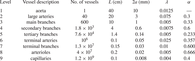
We consider dispersion of a passive scalar by an incompressible Newtonian fluid flowing through a bifurcating network. Our network choice is motivated by the cardiovascular system comprising a wide variety of vessels (table 1), whose diameter ranges from  $8\ \mathrm {\mu }\textrm {m}$ to
 $10$ mm (Zamir Reference Zamir1988; Adam Reference Adam2011). Because blood consists of particles (in particular, erythrocytes and leukocytes) suspended in plasma, its rheological behaviour changes as it transits through the cardiovascular network from larger to smaller vessels due to the Fahraeus–Lindqvist effect (Pries et al. Reference Pries, Secomb, Gaehtgens and Gross1990; Sriram et al. Reference Sriram, Intaglietta and Tartakovsky2014a). This phenomenon significantly affects radial transport through vessel walls and the flow profile. However, our analysis treats vessel walls as impermeable. Changes in viscosity, affecting the flow velocity profile, do not significantly change the average density of blood in vessels with diameter larger than
 $15\ \mathrm {\mu }\textrm {m}$ (Hellums et al. Reference Hellums, Nair, Huang and Ohshima1995; Sriram et al. Reference Sriram, Intaglietta and Tartakovsky2014a, and the references therein) and, with some reservations, as small as
 $8\ \mathrm {\mu }\textrm {m}$ (Goldman Reference Goldman2008). We restrict our analysis to vessels with diameter greater than
 $13.8\ \mathrm {\mu }\textrm {m}$.
Dimensions of the cardiovascular vessels (Zamir Reference Zamir1988; Adam Reference Adam2011). Here,  $\lambda = a / L$ is the ratio between the radius (
 $a$) and length (
 $L$) of a vessel; and
 $\alpha = a_{d} / a_{p}$ is the ratio between the radii of the daughter (
 $a_{d}$) and parent (
 $a_{p}$) vessels.

In large vessels of the cardiovascular network, flow is as periodic as the beating of the heart. In large arteries, flow is variable along the length of an artery as the vessel diameter tapers. Transport in such arteries must be modelled individually (Olufsen Reference Olufsen1999), as the geometry of the vessel and elasticity of the vessel wall have significant impacts on the pattern of fluid flow. However, further downstream, in the arteriolar tree, flow becomes steady (Green Reference Green and Glasser1944; Sarpkaya Reference Sarpkaya1966). These vessels, tertiary branches to arterioles, are a part of the arteriolar network that may be modelled as a fractal tree (Olufsen Reference Olufsen1999; Olufsen et al. Reference Olufsen, Peskin, Kim, Pedersen, Nadim and Larsen2000; Cousins & Gremaud Reference Cousins and Gremaud2012; Cousins et al. Reference Cousins, Gremaud and Tartakovsky2013). Based on the preceding discussion, we make the following assumptions about flow in the arteriolar tree:
(i) blood flow in arterioles behaves as a Newtonian fluid (Lee & Fung Reference Lee and Fung1971; Zimmerman et al. Reference Zimmerman, Tsai, Intaglietta and Tartakovsky2019);
(ii) the vessels are modelled as straight cylinders with rigid walls;
(iii) flow in arterioles is characterized by low Reynold's numbers and, as such, exhibits a laminar Poiseuille profile (Green Reference Green and Glasser1944; Sarpkaya Reference Sarpkaya1966); and
(iv) the arteriolar vessels are far downstream from the heart and the flow is well mixed (i.e. axial variations are negligible) and steady (Womersley Reference Womersley1955; Lee & Fung Reference Lee and Fung1971).
2.1. Fractal model of the arteriolar network
Following Olufsen (Reference Olufsen1999) and others, we adopt a fractal model of the arteriolar network in which each parent vessel of radius  $a$ bifurcates into two smaller daughter vessels. Each vessel generation bifurcates until a minimum radius
 $a_{min}$ is reached at the terminal daughter vessels. Murray's law states that the fractal arteriolar tree satisfies the principle of minimum work (Uylings Reference Uylings1977). It gives rise to a relationship between the radii of the parent (
 $a_{p}$) and daughter (
 $a_{{d}_1}$ and
 $a_{{d}_2}$) vessels,
 \begin{equation} a_{p}^{\zeta} = a_{{d}_1}^{\zeta} + a_{{d}_2}^{\zeta}. \end{equation}
The exponent  $\zeta$ is estimated to be
 $\zeta = 2.76$ in the human cardiovascular system (Olufsen Reference Olufsen1999).
Let  $\alpha _1$ and
 $\alpha _2$ denote the ratios between the radii of the daughter vessels and the radius of the parent vessel,
 \begin{equation} a_{{d}_1} = \alpha_1 a_{p}, \quad a_{{d}_2} = \alpha_2 a_{p}. \end{equation}
It follows from (2.1) and (2.2a,b) that
 \begin{equation} \alpha_1 = (1 + \psi^{\zeta})^{- 1 / \zeta}, \quad \alpha_2 = \psi \alpha_1, \quad \psi = a_{{d}_2} / a_{{d}_1}. \end{equation}
To simplify the presentation, we consider symmetric bifurcations, i.e. set the asymmetry ratio to  $\psi = 1$, so that
 $\alpha _1 = \alpha _2 \equiv \alpha = 2^{- 1 / \zeta }$. The fractal behaviour means that the parent–daughter scaling (2.2a,b) holds across all the generations,
 \begin{equation} \dfrac{a_{k+1}}{a_k} = \alpha = 2^{- 1 / \zeta}, \end{equation}
where  $k$ denotes the vessel generation.
2.2. Flow in fractal arteriolar networks
A relation for the flow velocities in the parent and daughter vessels is derived from the continuity equation. The mass flow rate,  $\dot {m}_k$, in a vessel of
 $k$th generation is given by
 \begin{equation} \dot{m}_k = \frac{\rm \pi}{4}\rho a_{k}^2 v_k, \end{equation}
where  $\rho$ is the fluid density and
 $v$ is the average flow speed (Darcy flux). For symmetrically bifurcating trees, mass continuity yields
 \begin{equation} \dot{m}_k = 2 \dot{m}_{k+1}. \end{equation}
We treat the fluid density  $\rho$ as constant throughout the entire arteriolar tree under consideration, because variations in density due to the Fahraeus–Lindqvist effect are minimal (Pries et al. Reference Pries, Secomb, Gaehtgens and Gross1990; Sriram et al. Reference Sriram, Intaglietta and Tartakovsky2014a). Combining (2.4)–(2.6), we obtain the relationship for flow speed in two adjacent generations,
 \begin{equation} v_{k+1} = \dfrac{v_k}{2 \alpha^2}. \end{equation}
3. Solute transport in individual vessels
Analytical solutions presented in this section express the concentration distribution within an individual vessel in terms of the (unknown, time-varying) nodal concentrations. The vessel's length and radius are  $L$ and
 $a$, respectively.
3.1. Problem formulation
Following Fung & Tang (Reference Fung and Tang1975) and Berg et al. (Reference Berg, Davit, Quintard and Lorthois2020) among many others, we assume that solute concentration in a single vessel,  $C(x,r,t)$, satisfies an advection–diffusion equation,
 \begin{equation} \frac{\partial C}{\partial t} = D_{m} \left[ \frac{1}{r}\frac{\partial}{\partial r} \left(r\frac{\partial C}{\partial r}\right)+\frac{\partial^2 C}{\partial x^2} \right] - u(r) \frac{\partial C}{\partial x}, \end{equation}
where  $x \in (0,L)$ and
 $r \in (0,a)$ are the axial and radial coordinates, respectively;
 $t > 0$ is time;
 $u(r)$ is the flow velocity given by the Poiseuille law; and
 $D_{m}$ is the coefficient of molecular diffusion. This equation is subject to initial and boundary conditions
 \begin{equation} \left. \begin{aligned} C(x,r,0) & = c_{in}, \quad C(0,r,t) = c_0(t), \quad C(L,r,t) = c_L(t), \\ C(x,0,t) & < \infty, \quad \frac{\partial C}{\partial r}(x,a,t) = 0. \end{aligned} \right\} \end{equation}
The last condition implies that vessel walls are impermeable to the solute. With the important caveats described in the Introduction, this assumption renders the results presented below relevant to such applications as targeted drug delivery (Shaw & Murthy Reference Shaw and Murthy2010); transport of some contrast agents used for in vivo molecular neuroimaging (Koffie et al. Reference Koffie, Farrar, Saidi, William, Hyman and Spires-Jones2011); and dispersion of large molecules such as PEG-haemoglobin and PEG-albumin proposed for use as blood substitutes (Cabrales et al. Reference Cabrales, Tsai, Winslow and Intaglietta2005) or high molecular weight hydroxyethyl starches used as plasma expanders (Dailey et al. Reference Dailey, Dysart, Langan, Slye, Nuttal, Schrader, Williams and Oliver2005). In these and other similar applications, the initial condition in (3.2a–e) represents a step concentration increase at the onset of an intervention. Finally, the imposition of the Dirichlet boundary conditions at the vessel's inlet and outlet facilitates the use of the solution to (3.1)–(3.2a–e) as a building block for the network solution developed in § 4.
For solutes that permeate vessel walls, the analytical solution of Zimmerman, Severino & Tartakovsky (Reference Zimmerman, Severino and Tartakovsky2018) can replace the solution to (3.1)–(3.2a–e) in the construction of the network solution.
3.2. Advection–dispersion equation
For physiologically relevant conditions,  $a \ll L$ and the radial dependence of solute concentration plays an insignificant role in the solute migration through the network. Therefore, we are interested in the dynamics of cross-sectionally averaged concentration
 \begin{equation} C_{av}(x,t) = \frac{2}{a^2} \int_0^a C(x,r,t) r\,\mathrm{d}r. \end{equation}
The latter satisfies an advection–dispersion equation (Aris Reference Aris1956)
 \begin{equation} \frac{\partial C_{av}}{\partial t} = D \frac{\partial^2 C_{av}}{\partial x^2} - v \frac{\partial C_{av}}{\partial x}, \quad v \equiv \frac{2}{a^2} \int_0^a u(r) r\,\mathrm{d}r, \quad D = D_{m} + \frac{v^2 a^2}{192D_{m}}. \end{equation}
This equation is subject to the initial and boundary conditions
 \begin{equation} C_{av}(x,0) = c_{in}, \quad C_{av}(0,t) = c_{0}(t), \quad C_{av}(L,t) = c_{L}(t). \end{equation}
Let  $L_{c}$,
 $v_{c}$,
 $D_{c}$ and
 $c_c$ denote the maximum values of the vessel length, Darcy velocity, dispersion coefficient and solute concentration in the network, respectively. We define dimensionless independent and dependent quantities,
 \begin{equation} \left. \begin{aligned} \bar{t} & = \frac{tD}{L_{c}^2}, \quad \bar{x} = \frac{x}{L_{c}}, \quad \bar{L} = \frac{L}{L_{c}}, \quad \bar{v} = \frac{v}{v_{c}}, \quad \bar{D} = \frac{D}{D_{c}}, \quad Pe = \frac{v_{c}L_{c}}{D_{c}},\\ \bar{C}_{av} & = \frac{C_{av}}{c_{c}}, \quad \bar{c}_{in}(\bar{x}) =\frac{c_{in}(\bar{x})}{c_{c}}, \quad \bar{c}_{L}(\bar{t}) =\frac{c_{L}(\bar{t})}{c_{c}}, \quad \bar{c}_{0}(\bar{t})=\frac{c_{0}(\bar{t})}{c_{c}}. \end{aligned} \right\} \end{equation}
A dimensionless form of (3.4a–c) and (3.5a–c) takes the form
 \begin{equation} \frac{\partial \bar{C}_{av}}{\partial \bar{t}} = \bar{D} \frac{\partial^2 \bar{C}_{av}}{\partial \bar{x}^2} - Pe \, \bar{v} \, \frac{\partial \bar{C}_{av}}{\partial \bar{x}}, \quad \bar x \in (0,\bar L), \quad \bar t > 0, \end{equation}
with
 \begin{equation} \bar{C}_{av}(\bar{x},0) = \bar{c}_{in}, \quad \bar{C}_{av}(0,\bar{t}) = \bar{c}_{0}(\bar{t}), \quad \bar{C}_{av}(\bar{L},\bar{t}) = \bar{c}_{L}(\bar{t}). \end{equation}
In the remainder of this study we utilize the dimensionless quantities but drop the bar  $\bar {\ \ }$ to simplify the notation.
3.3. Concentration distributions within a single vessel
We show in appendix A that the Laplace-transformed solution of (3.7) and (3.8a–c) is
 \begin{align} \hat{C}_{{av}}(x,s) &= \mathrm{e}^{\gamma x} \frac{ \sinh[(L-x)\varGamma] \hat{c}_0(s) + \mathrm{e}^{-\gamma L}\sinh(x\varGamma)\hat{c}_L(s) }{ \sinh(L\varGamma)}\nonumber\\ &\quad + \frac{2 D c_{in}}{L} \mathrm{e}^{\gamma x} \sum_{n=0}^{\infty} \omega_n \frac{ (-1)^n \textrm{e}^{-\gamma x} -1 }{\beta_n(s-\beta_n)} \sin(\omega_n x), \end{align}
where, for any function  $g(t)$,
 $\hat {g}(s) = \int _0^{\infty } g(t) \exp (-st)\,\mathrm {d}t$ denotes its Laplace transform; and
 \begin{equation} \beta_n = -D(\omega_n^2+\gamma^2),\quad \gamma = \frac{Pe\, v}{2D},\quad \omega_n = \frac{n {\rm \pi}}{L}, \quad \varGamma = \sqrt{\frac{s}{D}+\gamma^2}. \end{equation}
A benefit of working with the Laplace-transformed solution is its locality with respect to the Laplace-transformed inlet ( $\hat {c}_0$) and outlet (
 $\hat {c}_L$) boundary concentrations. That is in contrast to the non-local solution in the time domain, which
 $c_0(t)$ and
 $c_L(t)$ enter as convolutions. This feature becomes useful in building a network solution.
3.3.1. Steady-state solution
If the boundary concentrations  $c_0(t)$ and
 $c_L(t)$ have finite values at
 $t \rightarrow \infty$, then the steady-state solute concentration,
 $C_{av}^{ss}(x)$ is obtained from (3.9) by using the final value theorem,
 $C_{av}^{ss}(x) = \lim _{s \rightarrow 0} s \, \hat {C}_{av}(x,s)$,
 \begin{equation} C_{av}^{ss}(x) = \mathrm{e}^{\gamma x } \frac{ \sinh[(L-x)\gamma] c_0(\infty) + \mathrm{e}^{-\gamma L } \sinh (\gamma x) c_L(\infty) }{\sinh (\gamma L)}. \end{equation}
3.3.2. Solution for a semi-infinite vessel
Cousins et al. (Reference Cousins, Gremaud and Tartakovsky2013) assumed that the impedance at the network exit (i.e. at the end of the terminal arteriolar vessels) is negligible and that the network empties into an infinite reservoir, which represents the capillary microcirculation. One can model such an infinite reservoir as a semi-infinite vessel of the same diameter as the parent vessel, which would impose no resistance to the mass flow. The Laplace-transformed concentration profile in the semi-infinite vessel is (appendix A.3),
 \begin{equation} \hat{C}_{{av}}^{\infty}(x,s) = \left(\hat{c}_{0}(s)-\frac{c_{in}}{s}\right) \exp\left({\left(\gamma -\sqrt{\gamma^2+s/D}\right)x}\right) + \frac{c_{in}}{s}. \end{equation}
4. Solute transport in bifurcating networks
The finite-length solution (3.9) describes transport along a  $k$th generation vessel of a network, where the daughter-vessel inlet concentration
 $c_{0, k+1}(t)$ is imposed by the parent-vessel outlet concentration
 $c_{L,k}(t)$. Additionally, the daughter-vessel outlet condition is affected by the downstream impedance incurred from subsequent daughter vessels. The outlet condition in the terminal arterioles of the network may be unknown, but can be modelled by unimpeded flow into a large medium (Cousins & Gremaud Reference Cousins and Gremaud2012; Cousins et al. Reference Cousins, Gremaud and Tartakovsky2013). We describe this situation with the semi-infinite solution (3.11) for a vessel of the same diameter as the terminal vessels.
A nodal solution for transport throughout the tree, evaluated at bifurcation junctions, is developed by combining the tree model and the Laplace-transformed single-vessel solutions. Continuity of mass (concentration) and momentum (mass flux) is enforced at the junctions between a parent-vessel outlet and the respective daughter-vessel inlets.
4.1. Continuity conditions at network nodes
At each bifurcation point (node) in the  $k$th generation of the network, continuity of mass and momentum imposes conditions
 \begin{gather} \hat{C}_{{av},k}(L_{k},s) = \hat{C}_{{av},k+1}(0,s), \end{gather}
 \begin{gather} A_k \hat{J}_k(L_{k},s) = \sum_{m = 1}^{2}A_{k+1,m} \hat{J}_{k+1,m}(0,s), \end{gather}
respectively. Here  $A_k = {\rm \pi}a_k^2$ is the cross-sectional area of the
 $k$th generation vessel,
 $m$ identifies the daughter vessel branching from the parent vessel, and
 $J_k$ is the advective–dispersive mass flux across the
 $k$th interface,
 \begin{equation} J_{k}(x,t) = Pe_{k} v_{k} C_{{av},k}(x,t) - D_{k} \nabla C_{{av},k}(x,t). \end{equation}
For fractal networks, (4.2) simplifies to
 \begin{equation} \hat{J}_{k}(L_{k},s)= \sum_{m = 1}^{2}\alpha_m^2 \hat{J}_{k+1,m}(0,s), \quad \alpha_m = \frac{a_{k+1,m}}{a_k}. \end{equation}
4.2. Transport in symmetrically bifurcating networks
For symmetrically bifurcating networks, the continuity conditions (4.1) and (4.2) become
 \begin{equation} \hat{c}_{L,k}(s) = \hat{c}_{0,k+1,m}(s) \quad\text{and}\quad \hat{J}_k(L_k,s) = 2\alpha^2 \hat{J}_{k+1}(0,s), \end{equation}
where
 \begin{equation} \left. \begin{aligned} \hat{J}_{k}(L_{k},s) & = Pe_{k}v_{k}\hat{c}_{L,k}(s) - D_{k}\frac{\partial \hat{C}_{{av},k}(L,s)}{\partial x},\\ \hat{J}_{k+1}(0,s) & = Pe_{k+1}v_{k+1}\hat{c}_{0,k}(s) - D_{k+1}\frac{\partial \hat{C}_{{av},k+1}(0,s)}{\partial x}. \end{aligned} \right\} \end{equation}
Let  $\phi$ denote the nodal concentrations, such that
 $\phi _{k}$ is the parent-vessel inlet concentration,
 $\phi _{k+1}$ is the concentration at the parent-vessel to daughter-vessel interface, and
 $\phi _{k+2}$ is the daughter-vessel outlet concentration
 \begin{equation} \hat{\phi}_{k} = \hat{c}_{0,k},\quad \hat{\phi}_{k+1} = \hat{c}_{L,k} = \hat{c}_{0,k+1}, \quad \hat{\phi}_{k+2} = \hat{c}_{L,k+1}. \end{equation}
If the network consists of  $N_{gen}$ generations of vessels, then the finite vessel length solution (3.9) and the flux continuity in (4.5) give rise to a linear system of
 $N_{gen} - 1$ equations for the nodal concentrations,
 \begin{equation} \mathcal{A}_{k}\hat{\phi}_{k} + \mathcal{B}_{k}\hat{\phi}_{k+1} + \mathcal{F}_{k+1}\hat{\phi}_{k+2}= \mathcal{E}_{k}, \quad k = 1, \ldots, N_{gen}, \end{equation}
where
 \begin{equation} \left. \begin{aligned} \mathcal{A}_{k} & = \frac{D_{k}\varGamma_{k} \mathrm{e}^{\gamma_k L_k}}{\sinh(\varGamma_{k}L_{k})},\\ \mathcal{B}_{k} & = D_k \left[ \gamma_k -\varGamma_{k}\coth(\varGamma_{k}L_{k})\right] - 2 \alpha^2 D_{k+1} \left[\gamma_{k+1} +\varGamma_{k+1} \coth(\varGamma_{k+1}L_{k+1})\right],\\ \mathcal{E}_{k} & = \sum_{n=0}^{\infty} \sum_{j=k}^{k+1}2\omega_j^2\frac{(2 \alpha^2)^{j-k} c_{{in},j} }{L_{j}\beta_{j,n}(s-\beta_{j,n})} \left[1- (-1)^n \exp\left({(-1)^{j-k}\gamma_j L_j}\right) \right],\\ \mathcal{F}_{k} & = \frac{2 \alpha^2 \exp\left({-\gamma_k L_k}\right)D_{k}\varGamma_{k}}{\sinh(\varGamma_{k}L_{k})}. \end{aligned} \right\} \end{equation}
Since  $\phi _{1}$ and
 $\phi _{N_{gen}+1}$ are known boundary functions, this system has
 $N_{gen} - 1$ unknowns
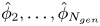 $\hat {\phi }_{2}, \ldots , \hat {\phi }_{N_{gen}}$. It is arranged in the form of a tridiagonal matrix for each value of
 $s$,
 \begin{equation} \begin{bmatrix} \mathcal{B}_{1} & \mathcal{F}_{2} & 0 & 0 & 0 & \cdots & 0\\ \mathcal{A}_{2} & \mathcal{B}_{2} & \mathcal{F}_{3} & 0 & 0 & \cdots & 0\\ 0 & \mathcal{A}_{3} & \mathcal{B}_{3} & \mathcal{F}_{4} & 0 & \cdots & 0\\ 0 & 0 & \mathcal{A}_{4} & \mathcal{B}_{4} & \mathcal{F}_{5} & \cdots & 0\\ \vdots & \vdots & & \ddots & \ddots & \ddots & \vdots\\ 0 & 0 & 0 & \cdots & \mathcal{A}_{N_{gen}-2} & \mathcal{B}_{N_{gen}-2} & \mathcal{F}_{N_{gen}-1} \\ 0 & 0 & 0 & \cdots & 0 & \mathcal{A}_{N_{gen}-1} & \mathcal{B}_{N_{gen}-1} \end{bmatrix} \begin{bmatrix} \hat{\phi}_{2} \\ \hat{\phi}_{3} \\ \hat{\phi}_{4} \\ \hat{\phi}_{5} \\ \hat{\phi}_{6} \\ \vdots \\ \hat{\phi}_{N_{gen}} \end{bmatrix} = \begin{bmatrix} \mathcal{E}_{1} -\mathcal{A}_{1}\hat{\phi}_{1} \\ \mathcal{E}_{2} \\ \mathcal{E}_{3} \\ \mathcal{E}_{4} \\ \mathcal{E}_{5} \\ \vdots \\ \mathcal{E}_{N_{gen}-1}-\mathcal{F}_{N_{gen}}\hat{\phi}_{N_{gen}+1} \end{bmatrix} \end{equation}
and solved using the Thomas algorithm (Datta Reference Datta2010).
If a network of finite-length vessels ends with a set of semi-infinite vessels at its last generation to incorporate the outflow condition, then
 \begin{equation} \left. \begin{aligned} \mathcal{A}_{N_{gen}-1} & = \frac{D_{N_{gen}-1}\varGamma_{N_{gen}-1} }{\sinh(\varGamma_{N_{gen}-1}L_{N_{gen}-1})} \exp\left({\gamma_{N_{gen}-1}L_{N_{gen}-1}}\right),\\ \mathcal{B}_{N_{gen}-1} & = D_{N_{gen}-1} [\gamma_{N_{gen}-1}-\varGamma_{N_{gen}-1}\coth(\varGamma_{N_{gen}-1}L_{N_{gen}-1}) ]-2 \alpha^2 (U_{N_{gen}}-D_{N_{gen}}\varpi),\\ \mathcal{E}_{N_{gen}-1} & = - \frac{\alpha^2c_{{in},N_{gen}}}{s}\varpi - 2 \omega_{N_{gen}-1}^2L_{N_{gen}-1}c_{{in},N_{gen}-1} \sum_{n=0}^{\infty} \frac{ 1-(-1)^n \exp\left({\gamma_{N_{gen}-1}L_{N_{gen}-1} }\right) }{ \beta_{N_{gen}-1,n}(s-\beta_{N_{gen}-1,n})},\\ \mathcal{F}_{N_{gen}} & = 0, \end{aligned} \right\} \end{equation}
where  $\varpi = \gamma _{N_{gen}}-\sqrt { \gamma _{N_{gen}}^2+ s/ D_{N_{gen}}}$.
5. Simulation results
5.1. Solute transport in a single vessel
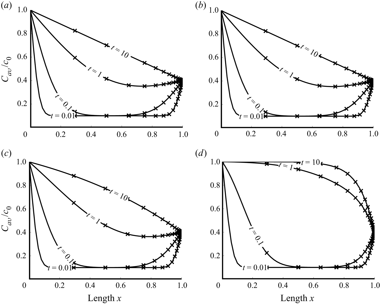
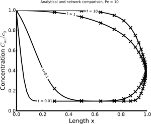
Distinct regimes of dispersive transport in a vessel are characterized by the Péclet number  $Pe = v_c L_c / D_c$, the ratio of the advective and dispersive time scales. Figure 1 exhibits temporal snapshots of concentration profiles
 $C_{av} / c_0$ for
 $Pe = 0.01$,
 $0.1$,
 $1.0$ and
 $10$. Recall that here and below all the quantities are dimensionless, as defined in (3.6a–j). The profiles for
 $Pe < 1$ are similar because dispersion (spreading of the front) dominates advection (translation of the front). The dispersive forces, therefore, drive the vessel saturation rate and small changes in the advective forces are not visible. As the Péclet number exceeds 1, the transport front becomes steeper, reflecting the increase in advective strength.
Temporal snapshots of the normalized concentration profiles,  $C_{av}(x,t) / c_0$, along the vessel,
 $0\le x \le 1$, for several values of the Péclet number,
 $Pe$. The profiles are computed, alternatively, with the analytical solution provided in appendix A (solid lines) and its counterpart obtained by numerical inversion of (3.9). The input concentrations are normalized with
 $c_0$, such that
 $c_L / c_0 = 0.4$ and
 $c_{in} / c_0 =0.1$. The network parameters are set to
 $N_{gen}=100$ and
 $\lambda = 0.1$.
 $(a)$
 $Pe = 0.01$.
 $(b)$
 $Pe = 0.1$.
 $(c)$
 $Pe = 1$.
 $(d)$
 $Pe = 10$.

The numerical error in our solution can stem only from numerical inversion of the Laplace transforms, which we have carried out with the DeHoog algorithm implemented by Hollenbeck (Reference Hollenbeck1998). Any numerical inversion algorithm loses accuracy near asymptotes, at early (large  $s$) and late (small
 $s$) times. The errors emerge as a result of numerical roundoff while performing operations with very large or small numbers (small
 $s$ correspond to large
 $t$, and vice versa). Additionally, they can vary with
 $Pe$ (Zimmerman, Jankowski & Tartakovsky Reference Zimmerman, Jankowski and Tartakovsky2016). These errors can be controlled either numerically by using systems/software that can handle larger floating point operations or analytically by evaluating the inverse Laplace transforms for small and large
 $s$, as is done in (3.10). Figure 1 demonstrates the agreement between the analytical solution for
 $C_{av}(x,t)$ and its counterpart obtained by numerical inversion of the Laplace transform
 $\hat {C}_{av}(x,s)$, for all values of
 $Pe$ considered.
5.2. Model verification
The data indicate that the ratio between vessel radius and vessel length is similar for both small and large vessels in the arteriolar network. We therefore assume that, in each generation  $k$, the length (
 $L_k$) and radius (
 $a_k$) of each vessel differ by the same constant (
 $\lambda$),
 \begin{equation} L_k = \dfrac{a_k}{\lambda}, \quad 0<\lambda<1. \end{equation}
To verify our network solution (4.8), we consider a network that is functionally equivalent to a single vessel. The network consists of  $N_{gen} = 100$ generations and has the same total length
 $L_{net}$ as the single vessel,
 $L_{net} = L = 1$. Since the total network length is
 \begin{equation} L_{net} = \sum_{k=1}^{N_{gen}} L_{k} = \sum_{k=1}^{N_{gen}} \frac{a_{k}}{\lambda}, \end{equation}
it follows from (2.4) that all vessels in the network have the aspect ratio
 \begin{equation} \lambda = \frac{ a_1 }{L_{net}} \sum_{k=1}^{\eta}\alpha^{k-1}. \end{equation}
The total cross-sectional area of each generation's vessel in the symmetrically bifurcating network is kept constant by choosing  $\alpha = 1/\sqrt {2}$. According to (2.7), this also ensures that the average flow velocity remains the same across all generations,
 $v_{k} = v_{k+1}$. The dispersion coefficient changes with velocity and vessel radius, in accordance with (3.4a–c). To facilitate verification of the semi-analytical network solution against the analytical single-vessel solution, we use the constant dispersion coefficient for all vessel generations,
 $D_{k} = D_{k+1}$. Transport in the network thus constructed should behave as though it were taking place in a single vessel of equivalent length and cross-sectional area. It is worthwhile emphasizing that this network does not represent the arterial tree; it merely serves to verify our network solution (4.8).
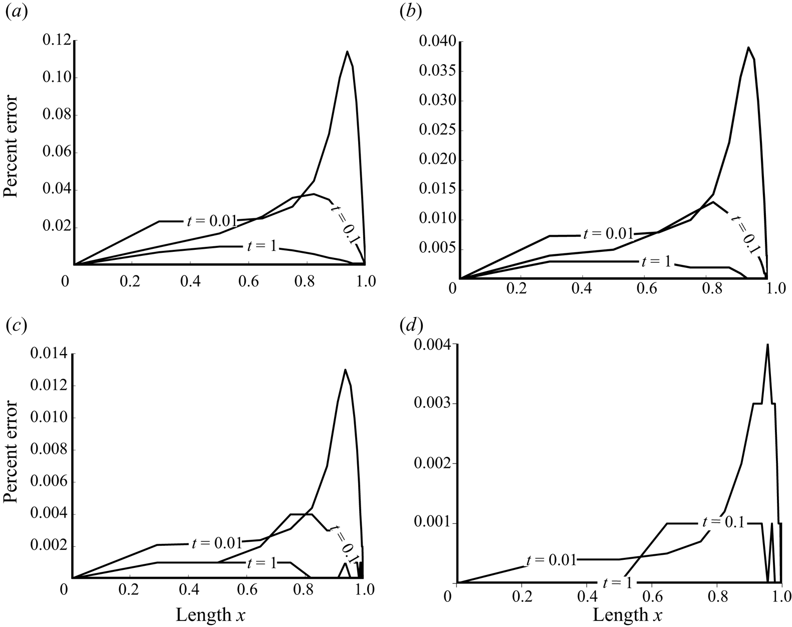
By construction, the concentration profiles are identical to those in figure 1. The relative error between the network solution (4.8) and the single-vessel solution (3.9),  $\varepsilon (x,t) = (C_{network} -C_{single}) / C_{single}$, is displayed in figure 2 for several values of the network Péclet number
 $Pe_{net}= v_{c} L_{tot} / D_{c}$. For all the scenarios considered, the error does not exceed
 $0.12\,\%$. It decreases with both time
 $t$ and
 $Pe$.
Relative error of the network solution. The model parameters are set to  $N_{gen}=100$,
 $\lambda = 0.1$,
 $c_L / c_0 = 0.4$ and
 $c_{in} / c_0 = 0.1$.
 $(a)$
 $Pe = 0.01$.
 $(b)$
 $Pe = 0.1$.
 $(c)$
 $Pe = 1$.
 $(d)$
 $Pe = 10$.

5.3. Analysis of a representative arteriolar network
A rigorous model of the human cardiovascular system should account for uneven bifurcation between parent and daughter vessels. The latter would require a solution for the impedance and pressure profiles of the network (Cousins & Gremaud Reference Cousins and Gremaud2012), as well as the changes in viscosity due to the Fahraeus–Lindqvist effect (Sriram et al. Reference Sriram, Intaglietta and Tartakovsky2014a). We present a methodology for deriving such a generalized model. Additionally, the dynamics of an evenly bifurcating network may inform the choice of more complex models. To demonstrate the transport behaviour in the evenly bifurcating arteriolar network, we consider two cases: a constant inlet and single-pulse inlet flow. The first utilizes a constant inlet boundary condition with no initial concentration to illustrate the development of a steady-state flow. The second implements a step function at the inlet boundary with no initial concentration to represent a single pulse of solute transiting through the network. In both cases, the unimpeded outflow boundary condition is imposed at the network exit, i.e. the vessel exit empties into a semi-infinite vessel of the same diameter.
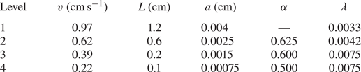
Table 1 collates the vessel geometric characteristics found throughout the human arterial vasculature. Our network model is built from the arteriolar parameters presented in table 2. For the exponent  $\zeta = 2.76$, representative of the human cardiovascular system (Olufsen Reference Olufsen1999), (2.4) predicts the daughter-to-parent radius ratio
 $\alpha = 0.778$. (This value is slightly above the values reported in table 2, which can be attributed to our choice of the symmetrical branching.) We set
 $\lambda = 0.005$, which is the median value of those reported in table 2 and is in agreement with its counterpart for the arteriolar vessels in table 1.
Dimensions of, and flow velocity in, vessels of the arteriolar network (Popel & Gross Reference Popel and Gross1979). Here,  $\lambda = a / L$ is the ratio between the radius (
 $a$) and length (
 $L$) of a vessel; and
 $\alpha = a_{d} / a_{p}$ is the ratio between the radii of the daughter (
 $a_{d}$) and parent (
 $a_{p}$) vessels.

The flow rate and vessel radius in the first arteriolar vessel generation ( $k=1$) is selected from table 2 to be
 $v_1 = 10\ \textrm {mm}\,\textrm {s}^{-1}$ and
 $a_1 = 40\ \mathrm {\mu }\textrm {m}$, respectively. The corresponding diffusion coefficient is chosen as
 $D_{m} = 10^{-4}\ \textrm {mm}^{2}\,\textrm {s}^{-1}$. We select the minimum vessel radius
 $a_{min} = 8\ \mathrm {\mu }\textrm {m}$, below which our arteriolar network is terminated and the unimpeded outflow condition is imposed. When used in conjunction with the fractal model of § 2, these vessel geometries and parameters result in a symmetrically bifurcating arteriolar tree with
 $N_{gen} = 8$ generations and
 $a_{N_{gen}} = 6.9\ \mathrm {\mu }\textrm {m}$.
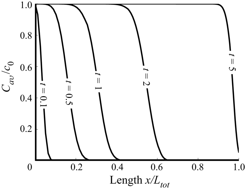
Figure 3 shows the propagation of the concentration front in the described arteriolar tree with zero initial concentration,  $c_{in} = 0$, a fixed inlet concentration,
 $c_0$, and the unimpeded outflow condition (4.9). The Péclet numbers observed in the arteriolar network are large, leading to the sharp concentration front at all times. At early times, the front develops its shape and widens. As the concentration front transits to the downstream vessels, the Péclet number of the daughter generations decreases, because
 $\alpha > 1/\sqrt {2}$, and so the collective cross-sectional area of each generation is greater than that of the parent generation. In a single vessel with constant cross-sectional area, a decrease in the Péclet number results in the dispersion phenomenon having a greater effect on the transport front of the solute. This can be inferred from the flow regime comparisons in figure 1. A lower Péclet number results in a more gradual concentration front when comparing vessels of similar geometry. Counterintuitively, the network presented in figure 3 has a concentration front that steepens as it transits toward the network exit. This phenomenon is due to reduced velocity of flow in each successive generation, which causes the concentration front to ‘bunch up’ similar to a traffic jam. As will be seen shortly, this effect is more pronounced with the single pulse inlet boundary condition.
Temporal snapshots of the normalized concentration profiles,  $C_{av}(x,t) / c_0$, along the length of the network with constant inlet concentration
 $c_0$ and initial concentration
 $c_{in} = 0$. The parameter values are set to
 $\lambda = 0.005$,
 $\alpha = 0.778$,
 $a_1 = 0.04\ \textrm {mm}$,
 $u_1 = 10\ \textrm {mm}\,\textrm {s}^{-1}$ and
 $D_{m} = 10^{-4}\ \textrm {mm}^{2}\,\textrm {s}$.

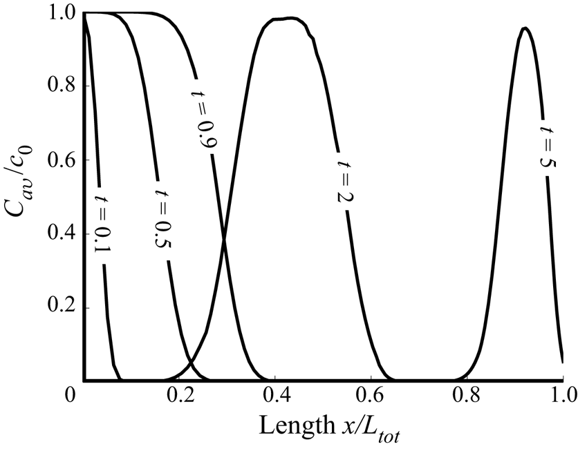
The second case is defined by a single pulse inlet boundary condition, zero initial concentration and the unimpeded flow boundary condition at the vessel exit. The pulse inlet boundary condition is a step function given by the relation
 \begin{equation} c_0(t) = \mathcal{A} [H(t-t_{1})-H(t-t_{2})]. \end{equation}
Here,  $t_{1}$ and
 $t_{2}$ are the times at which the pulse starts and ends,
 $\mathcal {A}$ is the concentration of the pulse and
 $H(\cdot )$ is the Heaviside step function. The Laplace transform of (5.4) is
 \begin{equation} \hat{c}_{0}(s)= \frac{\mathcal{A}}{s} \left[\mathrm{e}^{-t_{1}s} - \mathrm{e}^{-t_{2}s}\right]. \end{equation}
Figure 4 shows a one-second pulse introduced at the network's entrance. The network used in this case is geometrically and physiologically consistent with the constant inlet boundary condition case described in figure 3. The regime that resulted in the steepening of the transport front in figure 3 is also observable in figure 4. However, now, the trailing edge of the pulse ‘catches up’ with its leading edge, illustrating the traffic jam behaviour. At first glance, the solute appears to be lost because the area under the curve decreases as the pulse transits down the network. This phenomenon is due to the increase in cross-sectional area of each successive vessel generation as the pulse moves towards the network exit. Conversely, networks with  $\alpha < 1/\sqrt {2}$ induce transport fronts to grow wider as the Péclet number increases and the total cross-sectional area decreases with each successive generation.
Temporal snapshots of the normalized concentration profiles,  $C_{av}(x,t) / \mathcal {A}$, along the length of the network with initial concentration
 $c_{in} = 0$ and the pulse inlet concentration (5.4). The parameter values are set to
 $\lambda = 0.005$,
 $\alpha = 0.778$,
 $a_1 = 0.04\ \textrm {mm}$,
 $u_1 = 10\ \textrm {mm}\,\textrm {s}^{-1}$ and
 $D_{m} = 10^{-4}\ \textrm {mm}^{2}\,\textrm {s}^{-1}$.

6. Conclusions
We developed an analytical model for advection–dispersion transport in a fractal bifurcating network. The solution was evaluated for the values of geometric and topological parameters relevant to the human arteriolar vasculature. The accuracy of our solution, i.e. the errors associated with numerical inversion of Laplace transforms, was investigated over the physiologically relevant range of the parameter values.
Our analysis revealed that solute transport through an evenly bifurcating network is controlled, to a large extent, by the ratio ( $\alpha$) between the radii of the daughter and parent vessels. Specifically,
 $\alpha = 1/\sqrt {2}$ identifies an inflection point at which the transport behaviour changes. A network with
 $\alpha > 1/\sqrt {2}$ gives rise to a transport front that bunches up from a linear perspective of the vascular network. A network with
 $\alpha = 1/\sqrt {2}$ corresponds to Da Vinci's law, according to which the cross-sectional area of a parent tree branch (or tree trunk) is equal to the total cross-sectional area of the daughter branches; this regime is applicable to transport in xylem (Minamino & Tateno Reference Minamino and Tateno2014). Networks with
 $\alpha < 1/\sqrt {2}$ induce transport fronts to widen as the Péclet number increases and the total cross-sectional area decreases with each successive generation.
To focus on the effects of network topology on transport characteristics, we neglected many key features of transport in microcirculation such as a lattice-like structure of the capillary bed, radial transport through vessel walls, and non-Newtonian behaviour of blood in small vessels. In this sense, the relevance of our model to microcirculation comes with important caveats. It should be used as an abstracted representation of solute transport in the arteriolar network just upstream of the capillary bed, where the network exhibits fractal bifurcation patterns. Our single-vessel solutions can be replaced with the solutions of Zimmerman et al. (Reference Zimmerman, Severino and Tartakovsky2018) to account for diffusive losses through the vessel wall. They can be generalized further by replacing the Hagen–Poiseuille profile characteristic of Newtonian fluids with its counterparts resulting from the two-phase Newtonian (Sriram et al. Reference Sriram, Vazquez, Tsai, Cabrales, Intaglietta and Tartakovsky2012) or non-Newtonian (Sriram, Intaglietta & Tartakovsky Reference Sriram, Intaglietta and Tartakovsky2014b) models of blood in microcirculation. Finally, one can follow Cousins & Gremaud (Reference Cousins and Gremaud2012) to accommodate asymmetric bifurcations at each vessel junction, and Sriram et al. (Reference Sriram, Intaglietta and Tartakovsky2014a) to account for viscosity changes due to the Fahraeus–Lindqvist effect.
Our results are also applicable to transport in a variety of other environments such as nutrient transport in floral structures (Mäkelä Reference Mäkelä2002), fungal networks (Heaton et al. Reference Heaton, Obara, Grau, Jones, Nakagaki, Boddy and Fricker2012b) and drug delivery (Shipley & Chapman Reference Shipley and Chapman2010). Our model can be extended to networks with more than two daughter vessels branching per junction. Small modifications to the branching parameters, can describe a wide variety of other fractal networks.
Acknowledgements
This work was supported in part by Air Force Office of Scientific Research under award number FA9550-18-1-0474.
Declaration of interests
The authors report no conflict of interest.
Appendix A. Derivation of single-vessel solutions
We use the Green's function method to derive an analytical solution to (3.7) and (3.8a–c), and the Laplace transformation to obtain its counterpart for a semi-infinite vessel.
A.1. Greens’ function for advection–dispersion equation
The Green's function in (3.7) and (3.8a–c),  $G(x,\xi , t-\tau )$, satisfies an adjoint equation
 \begin{equation} \frac{\partial G}{\partial \tau} = D\frac{\partial^2 G}{\partial \xi^2} - Pe \, v\, \frac{\partial G}{\partial \xi} + \delta(x-\xi) \delta(t-\tau), \quad x,\xi \in (0,L), \quad t > \tau >0; \end{equation}
subject to homogeneous initial and boundary conditions
 \begin{equation} G(x,t;\xi,0) = 0, \quad G(x,t;0,\tau) = 0, \quad G(x,t;L,\tau) = 0, \end{equation}
where  $\delta (\cdot )$ is the Dirac delta function. The solution of this boundary-value problem is
 \begin{equation} G(x,\xi,t-\tau) = 2 H(t-\tau)\sum_{n=0}^{\infty} \exp\left({\beta_n(t-\tau)-\gamma(\xi-x)}\right) \sin(\omega_n x) \sin(\omega_n \xi), \end{equation}
where  $H(\cdot )$ is the Heaviside function; and the constants
 $\beta _n$,
 $\gamma$ and
 $\omega _n$ are defined in (3.9b).
A.2. Solution to advection–dispersion equation
The solution to (3.7) and (3.8a–c) is written in terms of the Green's function  $G(x,\xi , t-\tau )$ in (A 3) as
 \begin{align} C_{av}(x,t) = \int_{0}^{L} c_{in} G(x,\xi,t)\,\mathrm{d}\xi \!+\! \int_{0}^{t} \left[ c_{0}(\tau)\frac{\partial G}{\partial \xi}(x,0,t-\tau) -c_{L}(\tau)\frac{\partial G}{\partial \xi}(x,L,t-\tau)\right] \,\mathrm{d}\tau. \end{align}
For the spatially uniform initial concentration  $c_{in}$, substituting (A 3) into (A 4) and taking the Laplace transformation of the resulting expression, we obtain
 \begin{equation} \hat{C}_{{av}}(x,s) = \frac{2 D }{L} \mathrm{e}^{\gamma x} \sum_{n=0}^{\infty} \frac{\omega_n \sin(\omega_n x)}{s-\beta_n}\left[ c_{in} \frac{(-1)^n \mathrm{e}^{-\gamma L} - 1}{\beta_n} +\hat{c}_{0}(s)-(-1)^n \mathrm{e}^{-\gamma L}\hat{c}_{L}(s)\right]. \end{equation}
Since (Hansen Reference Hansen1975, equations (14.3.8) and (14.3.9))
 \begin{equation} \sum_{n=0}^{\infty} \frac{n}{n^2a^2+b^2} \sin(n X) = \frac{\rm \pi}{2 a^2} \frac{\sinh[({\rm \pi}-X)b/a]}{\sinh({\rm \pi} b/a)} \end{equation}
and
 \begin{equation} -\sum_{n=0}^{\infty} \frac{(-1)^n n }{n^2a^2+b^2} \sin(n X) = \frac{\rm \pi}{2 a^2} \frac{\sinh(b X/a)}{\sinh({\rm \pi} b / a )}, \end{equation}
Single-vessel solutions may be developed without the use of the Green's function method, as was done in the case of the semi-infinite vessel solution in § 3. In some cases these other methods may even present a more concise derivation. The Green's functions are utilized here for the purpose of presenting a base on which higher-dimensional solutions may be developed in future work. Specifically, the Green's function for a multi-dimensional advection–diffusion equation (e.g. in cylindrical coordinates) is given by the product of the corresponding one-dimensional Green's functions such as (A 3).
A.3. Solution for a semi-infinite vessel
In the case of a semi-infinite vessel, the domain of definition of (3.7),  $(0,L)$, is replaced with
 $(0,\infty )$, and the last boundary condition in (3.8a–c) with
 $C_{av}(\infty ,t) = c_{in}$.
The Laplace transform of (3.7) is
 \begin{equation} s\hat{C}_{{av}}(x,s) - c_{in} = \frac{\mathrm{d}^2 \hat{C}_{{av}}(x,s)}{\mathrm{d} x^2} - \frac{Pe\, v}{D} \frac{\mathrm{d} \hat{C}_{{av}}(x,s)}{\mathrm{d} x}. \end{equation}
A solution to this equation is a linear combination of homogeneous and particular solutions,
 \begin{equation} \hat{C}_{{av}}(x,s) = \hat{C}_{h}(x,s) + \hat{C}_{p}(x,s). \end{equation}
The former satisfies
 \begin{equation} s\hat{C}_{{h}}(x,s) = \frac{\mathrm{d}^2 \hat{C}_{{h}}(x,s)}{\mathrm{d} x^2} - \frac{Pe\, v}{D} \frac{\mathrm{d} \hat{C}_{{h}}(x,s)}{\mathrm{d} x} \end{equation}
and is given by
 \begin{equation} \hat{C}_{{h}}(x,s) = a_1 \mathrm{e}^{\theta_- x} + a_2 \mathrm{e}^{\theta_+ x}, \quad \theta_{\pm} = \gamma\pm\sqrt{\gamma^2+s/D}. \end{equation}
A particular solution to (A 8), obtained either by direct inspection of (A 8) or with the method of variation of parameters, is
 \begin{equation} \hat{C}_{p}(x,s) = \frac{c_{in}}{s}. \end{equation}
Accounting for the boundary conditions to compute the constants of integration  $a_1$ and
 $a_2$, we obtain (3.11).