1 Introduction
Shock-wave phenomenon is a fundamental topic in both high-speed flows and high-energy density physics. A deep understanding of how these sudden compressions form, evolve and interact with the surrounding flow and the propagating medium has been pivotal in the progress of many areas that include aerodynamics, propulsion, detonation science, ballistics, inertial confinement fusion and astrophysics, to name a few (Urzay Reference Urzay2018). The complexities that inherently appear in transonic flows have drawn the attention of the scientific community, as they have shown a proper identity characterized by the non-trivial acoustic coupling and the high nonlinearity of the governing equations. A common example is the shock reflection in flat plates, whose seemingly simple problem formulation in terms of the shock-jump equations fails at providing solutions in certain conditions, as first noticed by Mach (Reference Mach1878). The irregular configuration that arises when a single reflected shock does not suffice to provide mechanical equilibrium downstream involves the generation of triple-point shock confluences. Substantial progress followed after the pioneering theoretical work of von Neumann (Reference von Neumann1943a
,Reference von Neumann
b
), with those of Jones, Martin & Thornhill (Reference Jones, Martin and Thornhill1951) and Sternberg (Reference Sternberg1959) on the local nature of the triple point that deserve special recognition. Although large-scale properties of irregular reflections have been mostly studied through ideal-flow assumptions (Dewey & McMillin Reference Dewey and McMillin1985a
,Reference Dewey and McMillin
b
; Hornung Reference Hornung1986; Ben-Dor Reference Ben-Dor2007), the effect of the boundary layer, which is subsonic in the region closest to the wall, has been found to play a significant role in more intricate multiscale processes inside combustion chambers. This has led to the origin of the so-called
 $\unicode[STIX]{x1D706}$
-structure: a triple-shock configuration distinguishably different from the Mach stem (Henderson Reference Henderson1967; Grossman & Bruce Reference Grossman and Bruce2018). In particular, the viscosity-dominated layer, the lowest of the triple-deck structure that transversely extends up to zones of the order of
 $Re^{-5/8}$
times the streamwise coordinate (Nayfeh Reference Nayfeh1991), resolves the apparent paradox of upstream-moving information in the supersonic incoming stream. Resolution of the shock trajectory and the succeeding shock reflection in the vicinity of the plate needs an appropriate model to describe the distinguished regions within the boundary layer, with the triple-deck theory introduced by Lighthill (Reference Lighthill1953a
,Reference Lighthill
b
) and later on completed by Stewartson & Williams (Reference Stewartson and Williams1969). This problem is still subject to discussion, with the focus being recently placed on the effect of turbulence in the development of mixing layers (Dolling Reference Dolling2001; Pirozzoli & Bernardini Reference Pirozzoli and Bernardini2011; Jammalamadaka, Li & Jaberi Reference Jammalamadaka, Li and Jaberi2014; Adler & Gaitonde Reference Adler and Gaitonde2018; Quadros & Bernardini Reference Quadros and Bernardini2018; Estruch-Samper & Chandola Reference Estruch-Samper and Chandola2018).
In a parallel manner, the interaction of shock waves with contact surfaces that may result from stratified fluids, shear layers or mixing layers, has also been addressed from experimental, theoretical and numerical approaches. A well-known interaction of this type occurs when a planar shock crosses a perturbed interface that separates two different fluids, leading to the so-called Richtmyer–Meshkov instability (RMI). The study of this phenomenon has accumulated a large number of scientific publications in the past century since the pioneering works of Richtmyer (Reference Richtmyer1960) and Meshkov (Reference Meshkov1969). We refer to the recent works of Brouillette (Reference Brouillette2002), Nishihara et al. (Reference Nishihara, Wouchuk, Matsuoka, Ishizaki and Zhakhovsky2010) and references therein for further reading. The problem configuration suggests the use of linear theory to predict the growth rate of rippled interfaces at early times, as analytically developed by Wouchuk (Reference Wouchuk2001a ,Reference Wouchuk b ). By way of contrast, the interaction of oblique shocks with contact surfaces or tangential discontinuities can be addressed from linear theory when the strength of the former is sufficiently low (Riley Reference Riley1960; Huete et al. Reference Huete, Urzay, Sánchez and Williams2016) or the Mach number tangential discontinuity is weak enough (see appendix C). This type of interaction, despite comprising rich phenomena such as bifurcations in the convective Mach number domain, transonic regions, irregular reflections and unstable structures, has received much less attention to the best of the authors’ knowledge, with the works of Henderson (Reference Henderson1966), Henderson & Macpherson (Reference Henderson and Macpherson1968), Abd-El-Fattah, Henderson & Lozzi (Reference Abd-El-Fattah, Henderson and Lozzi1976), Abd-El-Fattah & Henderson (Reference Abd-El-Fattah and Henderson1978a ,Reference Abd-El-Fattah and Henderson b ), Skews & Ashworth (Reference Skews and Ashworth2005), Ben-Dor (Reference Ben-Dor2007) and Tesdall, Sanders & Keyfit (Reference Tesdall, Sanders and Keyfit2008) being some representative contributions in the limit of extremely thin contact surfaces. These works have established the basis to predict the type of irregular reflections that may arise attending to the structure shape. However, the study of the temporal evolution and the stability of the structure has received less consideration, in part due to the lack of experiments capable of covering sufficiently long periods. This fact motivates the work presented here, which aims to provide further insights into the time-dependent large-scale flow-field structures.
By virtue of the advances in numerical methods and high-fidelity simulations, the application of direct numerical simulation (DNS) and large eddy simulation (LES) to shear and mixing layers has permitted further understanding of these flows in turbulent conditions, see for instance the early works of Sandham & Reynolds (Reference Sandham and Reynolds1989) and Rogers & Moser (Reference Rogers and Moser1994). A remarkable contribution has been the analysis of the shear-layer growth rate for inert and reactive flows in different regimes of compressibility, as well as the characterization of turbulent structures developed within the two streams as a function of the convective Mach number. Although the vast majority of these numerical studies were carried out on temporally evolving layers as they require much less computational resources compared to spatially evolving layers, the latter strategy must be employed when the effect of the shock impingement on the mixing layer is to be investigated (Chaudhuri et al. Reference Chaudhuri, Hadjadj, Chinnayya and Palerm2011; Martínez-Ferrer et al. Reference Martínez-Ferrer, Buttay, Lehnasch and Mura2014; Fang et al. Reference Fang, Shen, Sun and Hu2018; Rao et al. Reference Rao, Asano, Imani and Saito2018).
The present work is focused on the study of the large-scale structures formed in the interaction of oblique shocks with shear layers. It extends the works of Henderson (Reference Henderson1966), Henderson & Macpherson (Reference Henderson and Macpherson1968) and Abd-El-Fattah & Henderson (Reference Abd-El-Fattah and Henderson1978a ,Reference Abd-El-Fattah and Henderson b ) addressing the irregular refraction problem from a combination of theoretical and numerical work. While the theoretical work provides a deeper understanding of the canonical problem and the explanation of its self-similar nature in time, the numerical simulations are used to describe the flow dynamics. The polar-plot method, the so-called Henderson–Neumann diagram, is employed to predict and to characterize flow-field structures that arise when the convective Mach number is sufficiently high to render non-steady configurations. The effect of the moving structure, along with real-gas effects, has been included in the polar-plot argumentation. Hereafter, real gas will refer to a thermally perfect gas with temperature-dependent heat capacities. The chart of irregular refractions based on the shape of the structure has been complemented with information about the temporal evolution. This evolution is found to be pseudosteady (of self-similar type) when the characteristic size is much larger than the shear thickness, yet smaller than the influencing domain. Results have been contrasted with high-fidelity numerical simulations performed with the code CREAMS that uses a fully compressible Navier–Stokes solver with a spatial seventh-order hybrid weighted essentially non-oscillatory (WENO) scheme and third-order total variation diminishing Runge–Kutta scheme. These computations provide valuable information that cannot be obtained from the hodograph plane: the description of the time-dependent response, the characterization of lengths of the generated Mach stems and the determination of the final flow-field structure among the multiple options predicted by the polar diagrams. The latter point has been previously addressed by less-energy-principle arguments (Henderson & Menikoff Reference Henderson and Menikoff1998) and also by solving the inner structure of the interaction, which ultimately determines the shock trajectory across the shear layer in supersonic-everywhere conditions (Whitham Reference Whitham1974; Martínez-Ruiz et al. Reference Martínez-Ruiz, Huete, Sánchez and Williams2018).
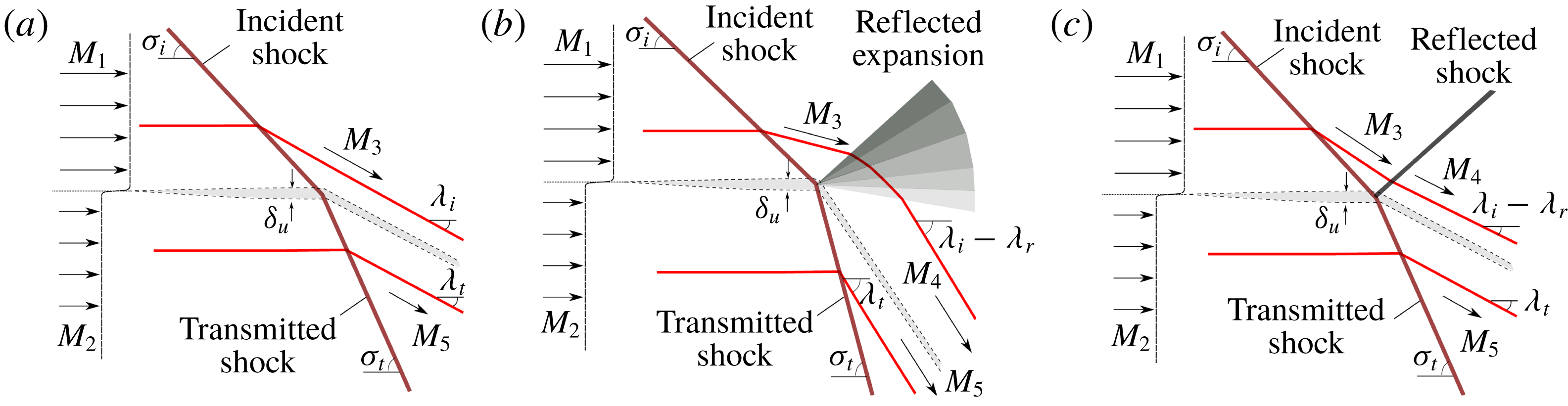
Sketch of regular shock/shear-layer interactions, (a) neutral transmission, (b) reflected rarefaction and (c) reflected shock.

The study considers the free-stream laminar configuration schematically shown in figure 1, which involves the interaction of a shear layer of thickness
 $\unicode[STIX]{x1D6FF}_{u}$
, separating two supersonic parallel streams with Mach numbers
 $M_{1}$
and
 $M_{2}$
, and an oblique shock with initial incident angle
 $\unicode[STIX]{x1D70E}_{i}$
. This shock is generated in the upper stream, that is the air stream in typical scramjet combustors (Urzay Reference Urzay2018), and transmitted to the lower stream with angle
 $\unicode[STIX]{x1D70E}_{t}$
. The simplest regular case, only involving incident and transmitted shocks, is the neutral transmission depicted in figure 1(a), where the exact upstream conditions are set to automatically provide equal pressure and deflection behind both shocks. In regular configurations involving a reflected expansion wave, see figure 1(b), the thin front curves locally while traversing the mixing layer as a consequence of the interaction with the non-uniform flow. This results in a shock inclination
 $\unicode[STIX]{x1D70E}(y)$
, with
 $y$
being the transverse coordinate that varies across the mixing layer. The value
 $\unicode[STIX]{x1D70E}=\unicode[STIX]{x1D70E}_{t}$
for
 $y<-\unicode[STIX]{x1D6FF}/2$
at the edge of the mixing layer corresponds to the transmitted-shock angle computed in Martínez-Ruiz et al. (Reference Martínez-Ruiz, Huete, Sánchez and Williams2018) using the method of characteristics at the inner mixing-layer region. Regular solutions may also call for a reflected shock wave, as shown in figure 1(c), which yields five uniform regions and three straight shocks in the steady asymptotic regime. However, in situations that exceed a critical condition for the convective Mach number
 $M_{1}$
–
 $M_{2}$
, the downstream region does not maintain mechanical equilibrium and the flow-field configuration is no longer steady. A curved shock wave is always transmitted and the shock/shear-layer intersection point continuously moves backwards, which is ultimately translated into different types of irregular structures whose sizes grow in time.
In contrast to boundary layers, where there exists a strong constraint in the slip-less condition at the wall, the shear-layer inner properties are expected to have a negligible impact on the large-scale structures since real-gas properties, like viscosity or thermal conductivity, become relevant at distances larger than the flow-field structures in high Reynolds number flows. In this limit, an inviscid coflow separated by an infinitely thin shear layer is considered. Therefore, the analysis assumes that the shear-layer evolution ahead of the shock impingement is negligible in a first approximation. Certainly, this might not be true if the shock is sufficiently far from the streams’ contact point, partly due to the Kelvin–Helmholtz instability triggered by the velocity shear that may eventually turn the initially laminar layer into a turbulent mixing layer (Rikanati et al. Reference Rikanati, Sadot, Ben-Dor, Shvarts, Kuribayashi and Takayama2006; Rubidge & Skews Reference Rubidge and Skews2014). However, as the convective Mach number may also be created by more stable configurations, as those involving same-velocity different-temperature streams, the focus is placed here on the large structures that are only dominated by the incident-shock angle and the stream Mach numbers.
The structure of the paper is as follows: the combinations of
 $M_{1}$
,
 $M_{2}$
and
 $\unicode[STIX]{x1D70E}_{i}$
that lead to regular conditions of mechanical equilibrium downstream from the shock are determined in § 2 by investigation of the related problem of shock-wave refraction at a contact surface. The limits to the regular conditions are also provided there. The effect of the moving shear layer structure and temperature-dependent heat capacity ratio is investigated in § 3. Irregular configurations are later analysed in § 4 with the aid of computational data validated with theoretical predictions based on polar-plot diagrams. The discussion of the results and a time-dependent analysis of the numerical simulations are provided in § 5. Finally, concluding remarks are offered in § 6. Appendix A details the numerical method employed, appendix B describes the polar-plot method for regular reflections and appendix C presents the linear theory for the interaction of oblique shocks with weak perturbations.
2 Regular configurations
An oblique shock traversing a supersonic stream, of Mach number
 $M$
and adiabatic index
 $\unicode[STIX]{x1D6FE}$
, with an angle
 $\unicode[STIX]{x1D70E}$
produces a net deflection of the flow of value
 $\unicode[STIX]{x1D706}=\unicode[STIX]{x1D706}(M,\unicode[STIX]{x1D70E},\unicode[STIX]{x1D6FE})$
, together with a change of its fluid properties such as temperature, density, pressure and Mach number. Furthermore, two coflowing streams under different upstream conditions are unevenly affected by the same traversing shock. The latter is accommodated in the lower stream by a transmitted angle
 $\unicode[STIX]{x1D70E}_{t}$
such that the downstream deflection of both currents must match and no pressure variations can be held across their contact surface. This far-field accommodation involves further reflected waves to meet mechanical equilibrium except for the degenerate case of neutral transmission.
For a given coflow configuration, made of the same gas with constant adiabatic index
 $\unicode[STIX]{x1D6FE}$
, the flow in the interaction region and the curvature of the shock discontinuity through the shear layer both depend on the Mach number distribution upstream of the shock, involving the boundary values
 $M_{1}$
and
 $M_{2}$
, and the inclination angle of the incident shock
 $\unicode[STIX]{x1D70E}_{i}$
. To determine the parametric domain
 $(M_{1},M_{2},\unicode[STIX]{x1D70E}_{i})$
, under which the resulting solutions correspond to those envisioned in figure 1, the outer-flow structure surrounding the interaction region is considered and assumes that the length scales are much larger than the shear-layer thickness
 $\unicode[STIX]{x1D6FF}_{u}$
. For these large scales, the shear layer appears infinitesimally thin, so that the problem reduces to that of the interaction of an oblique shock with a contact surface separating two supersonic streams. The outer-flow solution is independent of the Mach number profile across the shear layer ahead of the shock. This seemingly simple assumption admits in general multiple solutions depending on the values of the controlling parameters.
As discussed in Landau & Lifshitz (Reference Landau and Lifshitz1987), the simplest configurations are regular refractions involving straight-line waves, as sketched in figure 1. They involve a transmitted shock propagating from the impingement point into region-2, the lower stream, and a reflected wave propagating into region-3, the postshock stream of region-1. The reflected wave can either be a rarefaction or a shock that leaves different fluid conditions behind, both having been observed experimentally (Jahn Reference Jahn1956; Abd-El-Fattah et al. Reference Abd-El-Fattah, Henderson and Lozzi1976; Abd-El-Fattah & Henderson Reference Abd-El-Fattah and Henderson1978a ,Reference Abd-El-Fattah and Henderson b ; Buttsworth, Morgan & Jones Reference Buttsworth, Morgan and Jones1997). Therefore, a total of five regions of uniform flow are defined, where region-4 and region-5 are the downstream flow regions of the upper and lower streams respectively. In turn, these must coexist under the same deflected angle and pressure. These two types of regular refractions can only occur in certain ranges of the controlling parameters, beyond which more complicated irregular refraction patterns may arise. Theoretical considerations indicate that the ‘atlas’ of possible solutions include, in principle, single and double Mach reflections, 4-wave confluences and continuous expansion bands (Henderson Reference Henderson1966; Henderson & Macpherson Reference Henderson and Macpherson1968; Abd-El-Fattah et al. Reference Abd-El-Fattah, Henderson and Lozzi1976; Abd-El-Fattah & Henderson Reference Abd-El-Fattah and Henderson1978a ,Reference Abd-El-Fattah and Henderson b ), although only some of these solutions have been observed experimentally.
The above-mentioned regular refractions are composed by straight waves that delimit uniform regions of the flow. For the sake of simplicity, a single gas will be considered for both streams here, reducing the mixing-layer problem to a pure shear layer. When the shear-layer thickness is sufficiently small in comparison with any length scale representative of the flow-field domain besides the shock thickness, the regular solution is purely local and lacks a length scale. For example, the angle of the transmitted shock solely depends on the incoming flow conditions
 $M_{1}$
,
 $M_{2}$
, the adiabatic index
 $\unicode[STIX]{x1D6FE}$
and the shock incident angle
 $\unicode[STIX]{x1D70E}_{i}$
, thereby providing a constant value for
 $\unicode[STIX]{x1D70E}_{t}$
, i.e. the transmitted shock is a straight line. The solution of regular reflections, corresponding to given values of the input parameters
 $M_{1}$
,
 $M_{2}$
,
 $\unicode[STIX]{x1D6FE}$
and
 $\unicode[STIX]{x1D70E}_{i}$
, can be directly determined by application of jump conditions across the different waves in a zero-dimensional problem together with the compatibility conditions across the deflected contact surface. The Rankine–Hugoniot expressions for the pressure jump
 $$\begin{eqnarray}\displaystyle \hat{p}(M_{u},\unicode[STIX]{x1D70E},\unicode[STIX]{x1D6FE})=\frac{p}{p_{u}}=\frac{2\unicode[STIX]{x1D6FE}M_{u}^{2}\sin ^{2}\unicode[STIX]{x1D70E}+1-\unicode[STIX]{x1D6FE}}{\unicode[STIX]{x1D6FE}+1}, & & \displaystyle\end{eqnarray}$$
flow deflection angle
 $$\begin{eqnarray}\displaystyle \unicode[STIX]{x1D706}(M_{u},\unicode[STIX]{x1D70E},\unicode[STIX]{x1D6FE})=\tan ^{-1}\left\{\frac{2(M_{u}^{2}\sin ^{2}\unicode[STIX]{x1D70E}-1)\cot \unicode[STIX]{x1D70E}}{2+M_{u}^{2}[\unicode[STIX]{x1D6FE}+\cos (2\unicode[STIX]{x1D70E})]}\right\} & & \displaystyle\end{eqnarray}$$
and postshock Mach number
 $$\begin{eqnarray}\displaystyle M^{2}(M_{u},\unicode[STIX]{x1D70E},\unicode[STIX]{x1D6FE})=\frac{(\unicode[STIX]{x1D6FE}+1)^{2}M_{u}^{4}\sin ^{2}\unicode[STIX]{x1D70E}-4(M_{u}^{2}\sin ^{2}\unicode[STIX]{x1D70E}-1)(\unicode[STIX]{x1D6FE}M_{u}^{2}\sin ^{2}\unicode[STIX]{x1D70E}+1)}{(2\unicode[STIX]{x1D6FE}M_{u}^{2}\sin ^{2}\unicode[STIX]{x1D70E}+1-\unicode[STIX]{x1D6FE})[(\unicode[STIX]{x1D6FE}-1)M_{u}^{2}\sin ^{2}\unicode[STIX]{x1D70E}+2]}, & & \displaystyle\end{eqnarray}$$
are to be used for the shock waves involved in the flow, with the subscript
 $u$
denoting flow properties immediately upstream from the shock. In fact, for given values of
 $M_{1}$
and
 $\unicode[STIX]{x1D70E}_{i}$
, direct evaluation of these expressions provides
 $$\begin{eqnarray}\displaystyle \unicode[STIX]{x1D706}_{i}=\unicode[STIX]{x1D706}(M_{1},\unicode[STIX]{x1D70E}_{i},\unicode[STIX]{x1D6FE}),\quad p_{3}/p_{u}=\hat{p}(M_{1},\unicode[STIX]{x1D70E}_{i},\unicode[STIX]{x1D6FE}),\quad \text{and}\quad M_{3}^{2}=M^{2}(M_{1},\unicode[STIX]{x1D70E}_{i},\unicode[STIX]{x1D6FE})\quad & & \displaystyle\end{eqnarray}$$
across the incident shock, where
 $p_{u}=p_{1}=p_{2}$
is the pressure of the incoming streams, equal on both sides of the contact surface. On the other hand, across the transmitted shock
 $$\begin{eqnarray}\displaystyle \unicode[STIX]{x1D706}_{t}=\unicode[STIX]{x1D706}(M_{2},\unicode[STIX]{x1D70E}_{t},\unicode[STIX]{x1D6FE}),\quad p_{5}/p_{u}=\hat{p}(M_{2},\unicode[STIX]{x1D70E}_{t},\unicode[STIX]{x1D6FE})\quad \text{and}\quad M_{5}^{2}=M^{2}(M_{2},\unicode[STIX]{x1D70E}_{t},\unicode[STIX]{x1D6FE})\quad & & \displaystyle\end{eqnarray}$$
yield the downstream flow properties below the contact surface, involving the unknown value of the transmitted-shock angle
 $\unicode[STIX]{x1D70E}_{t}$
. When the reflected wave is a shock, the expressions for the jump between region-3 and region-4
 $$\begin{eqnarray}\displaystyle \unicode[STIX]{x1D706}_{r}=\unicode[STIX]{x1D706}(M_{3},\unicode[STIX]{x1D70E}_{r},\unicode[STIX]{x1D6FE}),\quad p_{4}/p_{3}=\hat{p}(M_{3},\unicode[STIX]{x1D70E}_{r},\unicode[STIX]{x1D6FE}),\quad \text{and}\quad M_{4}^{2}=M^{2}(M_{3},\unicode[STIX]{x1D70E}_{r},\unicode[STIX]{x1D6FE})\quad & & \displaystyle\end{eqnarray}$$
apply to the downstream flow properties above the contact surface. Correspondingly, equations (2.4), (2.5) and (2.6) along with the condition that imposes equal deflection angle and pressure along the streamlines, namely
 $$\begin{eqnarray}\displaystyle (p_{4}/p_{3})(p_{3}/p_{u})=(p_{5}/p_{u})\quad \text{and}\quad \unicode[STIX]{x1D706}_{t}=\unicode[STIX]{x1D706}_{i}-\unicode[STIX]{x1D706}_{r}, & & \displaystyle\end{eqnarray}$$
provide a set of eleven algebraic equations that determine
 $M_{3}$
,
 $M_{4}$
,
 $M_{5}$
,
 $\unicode[STIX]{x1D70E}_{r}$
,
 $\unicode[STIX]{x1D70E}_{t}$
,
 $\unicode[STIX]{x1D706}_{i}$
,
 $\unicode[STIX]{x1D706}_{r}$
,
 $\unicode[STIX]{x1D706}_{t}$
,
 $p_{3}/p_{u}$
,
 $p_{4}/p_{u}$
and
 $p_{5}/p_{u}$
as a function of
 $M_{1}$
,
 $M_{2}$
and
 $\unicode[STIX]{x1D70E}_{i}$
for a regular refraction with a reflected shock wave.
However, when the reflected wave is an expansion, the expressions detailed in (2.6) must be replaced, with
 $\unicode[STIX]{x1D70E}_{r}=\sin ^{-1}(M_{3})$
, by
 $$\begin{eqnarray}\displaystyle \left(\frac{p_{4}}{p_{3}}\right)^{(\unicode[STIX]{x1D6FE}-1)/\unicode[STIX]{x1D6FE}}=\frac{2+(\unicode[STIX]{x1D6FE}-1)M_{3}^{2}}{2+(\unicode[STIX]{x1D6FE}-1)M_{4}^{2}}\quad \text{and}\quad \unicode[STIX]{x1D706}_{r}=F_{PM}(M_{4})-F_{PM}(M_{3}), & & \displaystyle\end{eqnarray}$$
where
 $$\begin{eqnarray}\displaystyle F_{PM}(M)=\left(\frac{\unicode[STIX]{x1D6FE}+1}{\unicode[STIX]{x1D6FE}-1}\right)^{1/2}\tan ^{-1}\left\{\left[\frac{\unicode[STIX]{x1D6FE}-1}{\unicode[STIX]{x1D6FE}+1}(M^{2}-1)\right]^{1/2}\right\}-\tan ^{-1}[(M^{2}-1)^{1/2}] & & \displaystyle\end{eqnarray}$$
is the Prandtl–Meyer (PM) function for a supersonic expansion. In this case, the computation involves (2.4), (2.5), (2.7) and (2.8), with
 $-\unicode[STIX]{x1D706}_{r}$
replaced by
 $+\unicode[STIX]{x1D706}_{r}$
in the second equation of (2.7), which corresponds to the clockwise deflection associated with the reflected rarefaction. The values of the Mach number behind the reflected wave
 $M_{4}$
and behind the transmitted wave
 $M_{5}$
bound the shear layer from above and from below, respectively.
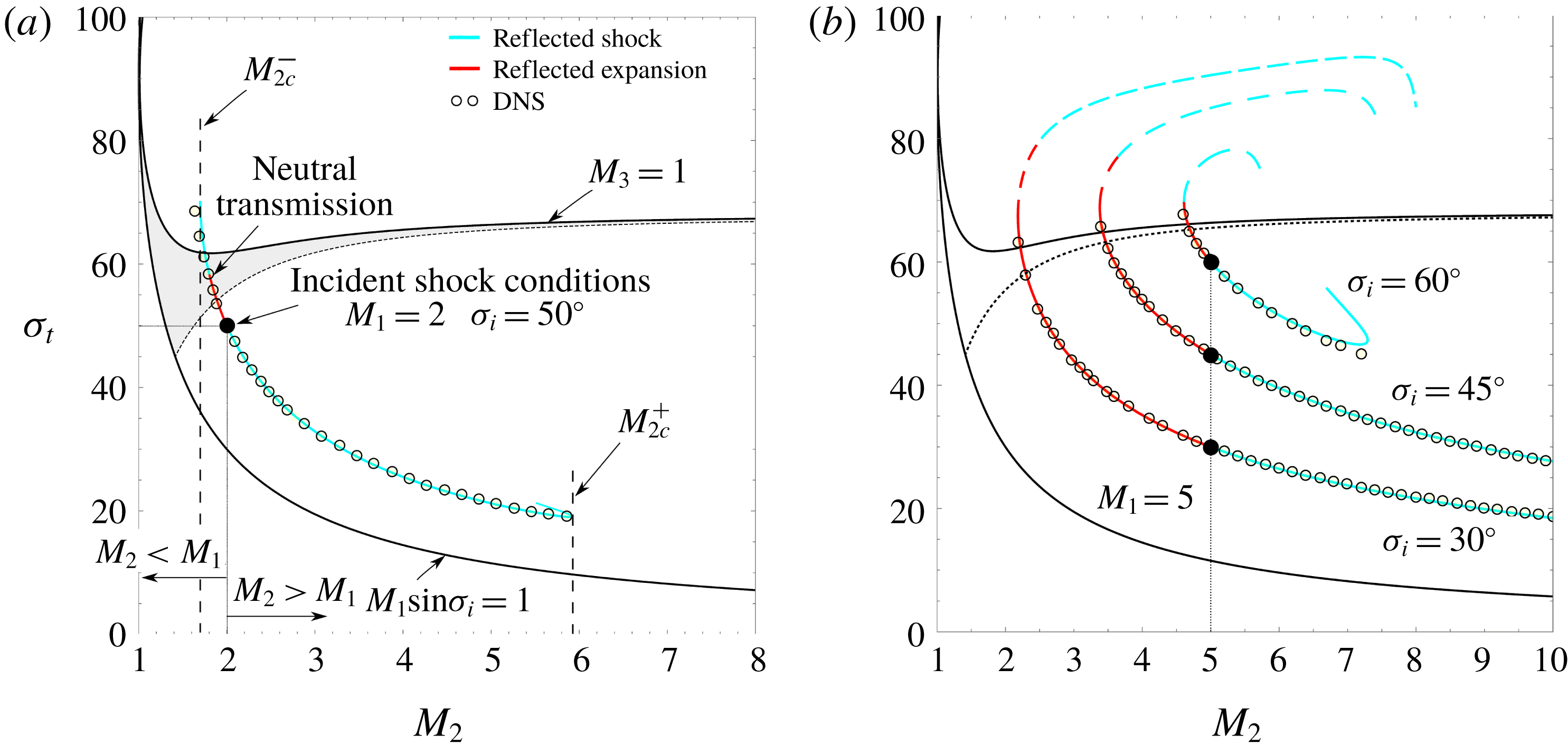
Transmitted-shock angle versus Mach number diagram given by (a) the outer problem for a stream
 $M_{1}=2$
and incident-shock angle
 $\unicode[STIX]{x1D70E}_{i}=50^{\circ }$
and (b) the comparison between the outer problem and highly resolved inviscid simulations for
 $M_{1}=5$
and
 $\unicode[STIX]{x1D70E}_{i}=30^{\circ }$
,
 $45^{\circ }$
and
 $60^{\circ }$
. Dashed curves represent the unstable branch of the multi-valued solutions.

Different sets of possible regular solutions are shown in figure 2 over the domain of transmitted-shock angle versus stream-2 Mach number. First, a trivial uniform flow field is denoted by a solid circle, where the transmitted solution matches the selected incident-shock conditions
 $M_{1}=M_{2}$
and
 $\unicode[STIX]{x1D70E}_{i}=\unicode[STIX]{x1D70E}_{t}$
. The possible locations of the upper-stream incident conditions are bounded by the lower solid line that represents the weak-shock limit,
 $M_{1}\sin \unicode[STIX]{x1D70E}_{i}=1$
, below which no shock would arise. In addition, cases over the
 $M_{3}=1$
line would produce subsonic postshock conditions behind the incident shock. Moreover, the colour curves define the collection of transmitted-shock angles
 $\unicode[STIX]{x1D70E}_{t}$
that comply with the problem equations for different values of
 $M_{2}$
and the upstream parameters (
 $M_{1}$
,
 $\unicode[STIX]{x1D70E}_{i}$
).
As soon as
 $M_{2}\neq M_{1}$
, the solution generally produces either a reflected compression or a reflected expansion wave, due to the combined effects of the convective Mach number and the intensity of postshock Mach waves impinging back on the shock. However, given an infinitesimally small convective Mach
 $\unicode[STIX]{x1D6FF}M=M_{2}-M_{1}$
, the postshock effects can be neglected as discussed in appendix C. In that limit, and given that
 $\unicode[STIX]{x1D6FF}M>0$
, compressions leading to a reflected shock are found inside the white island and expansions inside the shaded region of figure 2(a). In turn, the inverse behaviour is found if
 $\unicode[STIX]{x1D6FF}M<0$
, expansions in the white region and compressions in the shaded region. Nevertheless, for non-negligible values of
 $\unicode[STIX]{x1D6FF}M$
, the effects of Mach waves reaching the front from behind must be considered. Therefore, the previously mentioned regions are only approximately valid as a cumulative effect of differential increments or decrements of
 $M_{2}$
with respect to
 $M_{1}$
. Resolution of the set of equations renders multiple solutions associated with the configurations that provide mechanical equilibrium downstream. Consequently, in figure 2(a) transmitted solutions are plotted in cyan for reflected shocks (
 $M_{2}>M_{1}$
) and in red for reflected expansions (
 $M_{2}<M_{1}$
). However, the differential expansion contributions to the
 $M_{2}<M_{1}$
points balance out with the differential compressions that appear once into the shaded area to yield a neutral transmission point and, further, reflected-shock solutions.
In addition, three different scenarios with
 $M_{1}=5$
are represented in figure 2(b), namely
 $\unicode[STIX]{x1D70E}_{i}=30^{\circ }$
,
 $45^{\circ }$
and
 $60^{\circ }$
. A comparison of the transmitted angle
 $\unicode[STIX]{x1D70E}_{t}$
is displayed in dependence on
 $M_{2}$
between numerical simulations (symbols), and the theoretical outer problem (solid lines). The transmitted angle provided by simulations fits reasonably well with Landau’s outer solution, a result that is also extended to any other fluid property such as pressure or deflection angle. Red curves in figure 2(b) represent the solution predicted by a reflected-expansion configuration while cyan curves refer to shock-reflected cases.
Note that the set of solutions given by the regular-problem equations is multi-valued in some regimes, involving further branches of secondary solutions for
 $M_{2}$
such as the ones computed in the dashed upper curves in figure 2(b), which yield larger angles of the transmitted shock. The two-valued solution suggests two candidates for the final solution in a certain region. Multiplicity in the solutions can be solved by stability criteria (Fowles Reference Fowles1981). This may be more easily seen in the hodograph plane as shown in appendix B. There, the so-called pressure-deflection polar plots are computed by solving the inviscid problem, as proposed by Landau. This method, first introduced by von Neumann (Reference von Neumann1943a
,Reference von Neumann
b
) and later extended by Henderson (Reference Henderson1966), Henderson & Macpherson (Reference Henderson and Macpherson1968), is particularly useful to determine all possible solutions that ultimately lead to mechanical equilibrium in the downstream shear layer, i.e. when the upper and lower postshock streams propagate with the same pressure and direction. Additionally, highly resolved inviscid simulations have been used in this work to confirm the unstable nature of the upper branch in figure 2(b). Such numerical computations, whose results have not been displayed here for the sake of conciseness, have been initiated with the results predicted by (2.1)–(2.9). When the lower-branch predictions of (2.1)–(2.9) are employed as initial conditions, the numerical simulations rapidly accommodate to provide the stable results shown in figure 2(b) in good agreement. It must be noted that, in the numerical simulations, the adiabatic index depends on temperature (see appendix A) to meet the correction requirements of the irregular reflections studied below. There, large Mach numbers and flows including multiple shocks combined with expansions produce non-negligible changes in the adiabatic index. However, for regular intersections, small deviations are produced by these effects between the regular theoretical model for a calorically perfect gas (see appendix B) and the numerical solutions.
Critical values (
 $M_{2c}^{-}/M_{2c}^{+}$
) for the lower-stream Mach number predicted by Landau’s outer-problem equations when
 $\unicode[STIX]{x1D6FE}=1.4=\text{const}$
. Starred values refer to shock-reflected configurations, non-starred values refer to expansion-reflected cases and superscript
 $N$
refers to neutral transmission. The dash symbol means ‘not found’ within the interval
 $M_{2}=(1,20)$
.

The limits of the regular configurations are readily identified in the turning points of the curves. Due to the maximum deflection that can be produced by an oblique shock over a supersonic stream of a given Mach number plus a reflected wave, the downstream conditions of parallel isobaric flow cannot be met for any desired combination of
 $M_{1}$
,
 $M_{2}$
and
 $\unicode[STIX]{x1D70E}_{i}$
. Therefore, critical values of the lower stream
 $M_{2c}^{+}$
and
 $M_{2c}^{-}$
are found in both panels of figure 2, beyond which no regular solutions can be recovered by the system of (2.1)–(2.9). These limits, and those predicted by the intersection criteria of polar plots are, indeed, the same conditions. For the sake of completeness, lower and upper limits in terms of
 $M_{2}$
are identified as a function of
 $M_{1}$
and
 $\unicode[STIX]{x1D70E}_{i}$
, see table 1. Starred values refer to shock-reflected configurations and non-starred values refer to expansion-reflected cases. The superscript
 $N$
denotes a case of neutral transmission. The dash symbol means not found within the interval
 $M_{2}\in [1,20]$
, following the fact that
 $M>20$
is impractical and not normally encountered in applications. For instance, the curve corresponding to
 $M_{1}=5$
and
 $\unicode[STIX]{x1D70E}_{i}=60^{\circ }$
in figure 2(b) exhibits two turning points at
 $M_{2c}^{-}=4.61$
and
 $M_{2c}^{+}=7.3$
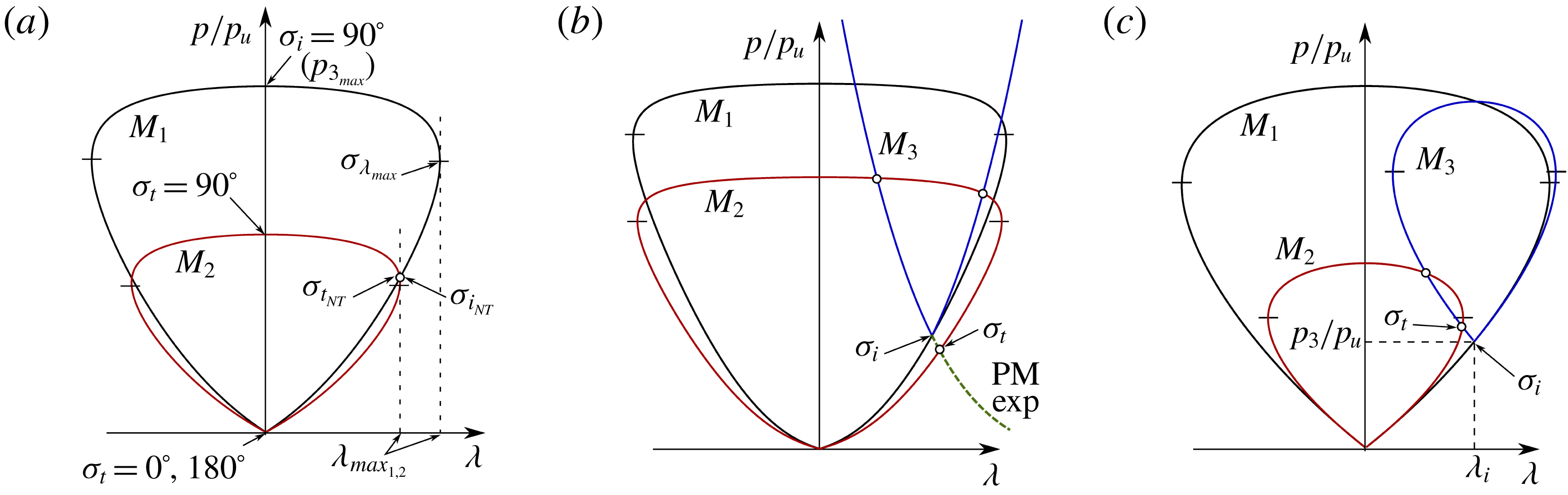
. These limits can be easily anticipated by analysing the hodograph plane, as described in appendix B. The cases where
 $M_{2}<M_{2c}^{-}$
correspond to situations for which the stream-2 polar in figure 18(b) is sufficiently small so that intersections do not occur either with the stream-3 polar or a Prandtl–Meyer expansion. On the other hand, situations where
 $M_{2}>M_{2c}^{+}$
correspond to a stream-2 polar sufficiently narrow that it does not intersect with the
 $M_{3}$
-loop.
3 Unsteady and real-gas considerations
We must accept that small perturbations in the convective Mach number beyond critical limits will produce a lack of equilibrium that fails to deflect the flow consistently. In this fashion, new structures make an appearance after impingement on the shear layer involving curved shocks, triple points, shock intersections, subsonic non-uniform regions and growing finite-length shocks that result from the unsteady flow field. Following Henderson (Reference Henderson1966), Henderson & Macpherson (Reference Henderson and Macpherson1968), the term Mach stem, that was first coined in the context of shock reflection in solid walls, will also be employed here to address the finite-length shocks that emerge in irregular interactions.
Under conditions that render subsonic flow behind the incident shock,
 $M_{3}<1$
, irregular configurations are found to be strongly affected by the upper-stream local boundaries, which are typically responsible for the incident-shock creation. This was inferred from the experiments in Abd-El-Fattah & Henderson (Reference Abd-El-Fattah and Henderson1978a
,Reference Abd-El-Fattah and Henderson
b
), namely bound precursor refraction and lambda shock refraction configurations. Nevertheless, when
 $M_{3}>1$
and the downstream boundary conditions are sufficiently far to affect the dynamics of the structure through any other subsonic region, the local flow field is self-similar as it lacks characteristic length scales. Therefore, the finite length of the Mach stem must scale with time, growing with the whole interacting structure. The associated movement is performed against the flow, so that the effective Mach number that is perceived at the shock surface is increased sufficiently to provide an equilibrium closure in pressure and deflection. In the hodograph plane, the corrected related polars are slightly larger, such that intersecting solutions independent of time are provided anew. This fact forces the contact point between the shear layer and shock structure to retreat at constant speed. A direct consequence being that self-similar constructions are achieved, where angles and downstream conditions are maintained constant.
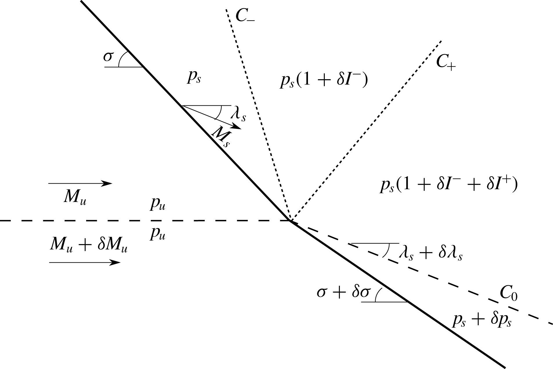
Previous works making use of the hodograph method did not include the effects of moving structures or temperature-dependent heat capacities, which we present here. Following this approach, an asymptotic analysis is developed for small perturbations on the post-shock adiabatic index
 $\unicode[STIX]{x1D6FF}\unicode[STIX]{x1D6FE}$
and inflow Mach number
 $\unicode[STIX]{x1D6FF}M$
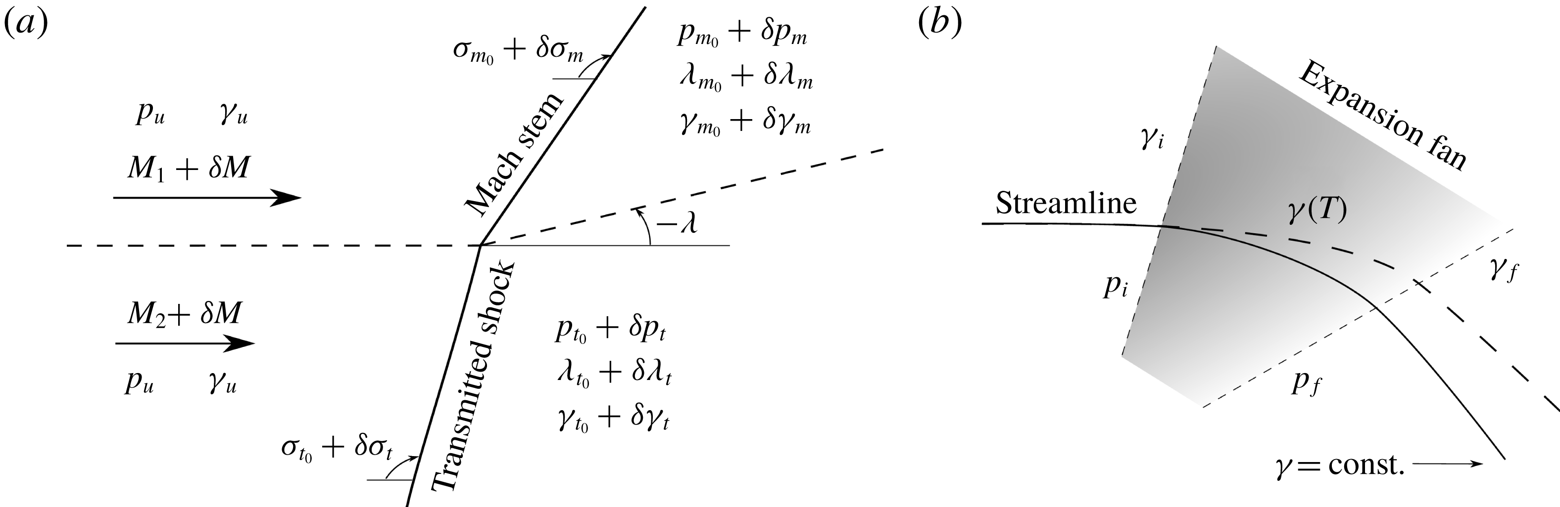
, which produce necessary second-order corrections to the pressure and deflection equilibrium conditions, as sketched in figure 3(a).
In the absence of viscous and conductive effects, the effect of temperature only enters into play via the heat capacity ratio
 $\unicode[STIX]{x1D6FE}$
, whose temperature dependence has been taken into account in the numerical simulations through the JANAF polynomials (see appendix A). Direct inspection of the Rankine–Hugoniot equations in the strong-shock limit can be used to provide an upper limit for the maximum temperature achieved for non-reactive cases. As
 $\unicode[STIX]{x1D6FE}$
may vary down to
 $6\,\%$
within the range of shock-induced temperature change considered, linear perturbations can be used to predict variations by an amount of order
 $\unicode[STIX]{x1D6FF}(\unicode[STIX]{x1D70C}/\unicode[STIX]{x1D70C}_{u})\sim -\unicode[STIX]{x1D6FE}/(\unicode[STIX]{x1D6FE}^{2}-1)\unicode[STIX]{x1D6FF}\unicode[STIX]{x1D6FE}\sim 10\,\%$
for the mass-compression ratio across one single shock. For a shock-train structure, this effect accumulates, with the value of
 $\unicode[STIX]{x1D6FF}\unicode[STIX]{x1D6FE}$
being properly modelled with the local temperature.
The mass-compression ratio for a gas that is not calorically perfect reads
 $$\begin{eqnarray}\displaystyle {\mathcal{R}} & = & \displaystyle \frac{\unicode[STIX]{x1D70C}}{\unicode[STIX]{x1D70C}_{u}}=\frac{\unicode[STIX]{x1D6FE}_{s}(\unicode[STIX]{x1D6FE}_{u}-1)(1+\unicode[STIX]{x1D6FE}_{u}M_{u_{n}}^{2})}{[2+(\unicode[STIX]{x1D6FE}_{u}-1)M_{u_{n}}^{2}]}\nonumber\\ \displaystyle & & \displaystyle +\,\frac{\sqrt{(\unicode[STIX]{x1D6FE}_{u}-1)[(\unicode[STIX]{x1D6FE}_{u}-1)\unicode[STIX]{x1D6FE}_{u}^{2}M_{u_{n}}^{4}+2\unicode[STIX]{x1D6FE}_{u}(\unicode[STIX]{x1D6FE}_{u}-\unicode[STIX]{x1D6FE}_{s}^{2})M_{u_{n}}^{2}+\unicode[STIX]{x1D6FE}_{s}^{2}(\unicode[STIX]{x1D6FE}_{u}-1)]}}{[2+(\unicode[STIX]{x1D6FE}_{u}-1)M_{u_{n}}^{2}]},\end{eqnarray}$$
where
 $M_{u_{n}}=M_{u}\sin \unicode[STIX]{x1D70E}$
, is the normal component of the Mach number, and
 $\unicode[STIX]{x1D6FE}_{u}$
and
 $\unicode[STIX]{x1D6FE}_{s}$
are, respectively, the upstream and post-shock values of the adiabatic index. Automatically, it follows that
 $$\begin{eqnarray}\displaystyle \hat{p}=1+\unicode[STIX]{x1D6FE}_{u}M_{u_{n}}^{2}(1-{\mathcal{R}}^{-1})\quad \text{and}\quad \unicode[STIX]{x1D706}=\unicode[STIX]{x1D70E}-\tan ^{-1}\left(\frac{\tan \unicode[STIX]{x1D70E}}{{\mathcal{R}}}\right). & & \displaystyle\end{eqnarray}$$
(a) Sketch of the moving contact point for
 $M_{2}<M_{2c}^{-}<M_{1}$
in a shock-anchored reference frame. The shock angles and the post-shock deflection angle usually reverse for
 $M_{2}>M_{2c}^{+}>M_{1}$
. (b) Sketch of the deflected streamline corrected by variable
 $\unicode[STIX]{x1D6FE}(T)$
in the expansion fan.

Regardless the type of irregular interaction, the contact-point properties are always determined by the local equilibrium downstream,
 $p_{5}=p_{6}$
and
 $\unicode[STIX]{x1D706}_{5}=\unicode[STIX]{x1D706}_{6}$
, which yields
 $\unicode[STIX]{x1D70E}_{m}$
and
 $\unicode[STIX]{x1D70E}_{t}$
as the local values of the oblique Mach stem and the transmitted shock. Therefore, small variations
 $\unicode[STIX]{x1D6FF}\unicode[STIX]{x1D6FE}_{m}$
and
 $\unicode[STIX]{x1D6FF}\unicode[STIX]{x1D6FE}_{t}$
are taken into account with respect to the downstream value
 $\unicode[STIX]{x1D6FE}_{s}=\unicode[STIX]{x1D6FE}_{m}$
and
 $\unicode[STIX]{x1D6FE}_{s}=\unicode[STIX]{x1D6FE}_{t}$
behind each shock, yielding the following perturbations to the shock angles
 $$\begin{eqnarray}\displaystyle \frac{\unicode[STIX]{x1D6FF}\unicode[STIX]{x1D70E}_{m}}{\unicode[STIX]{x1D6FF}\unicode[STIX]{x1D6FE}_{m}}=\frac{\hat{p}_{\unicode[STIX]{x1D70E}}|_{t}\left(\unicode[STIX]{x1D706}_{\unicode[STIX]{x1D6FE}}|_{t}\displaystyle \frac{\unicode[STIX]{x1D6FF}\unicode[STIX]{x1D6FE}_{t}}{\unicode[STIX]{x1D6FF}\unicode[STIX]{x1D6FE}_{m}}-\unicode[STIX]{x1D706}_{\unicode[STIX]{x1D6FE}}|_{m}\right)+\unicode[STIX]{x1D706}_{\unicode[STIX]{x1D70E}}|_{t}\left(\hat{p}_{\unicode[STIX]{x1D6FE}}|_{m}-\hat{p}_{\unicode[STIX]{x1D6FE}}|_{t}\displaystyle \frac{\unicode[STIX]{x1D6FF}\unicode[STIX]{x1D6FE}_{t}}{\unicode[STIX]{x1D6FF}\unicode[STIX]{x1D6FE}_{m}}\right)}{\hat{p}_{\unicode[STIX]{x1D70E}}|_{t}\unicode[STIX]{x1D706}_{\unicode[STIX]{x1D70E}}|_{m}-\hat{p}_{\unicode[STIX]{x1D70E}}|_{m}\unicode[STIX]{x1D706}_{\unicode[STIX]{x1D70E}}|_{t}} & & \displaystyle\end{eqnarray}$$
and
 $$\begin{eqnarray}\displaystyle \frac{\unicode[STIX]{x1D6FF}\unicode[STIX]{x1D70E}_{t}}{\unicode[STIX]{x1D6FF}\unicode[STIX]{x1D6FE}_{m}}=\frac{\unicode[STIX]{x1D706}_{\unicode[STIX]{x1D70E}}|_{m}\left(\hat{p}_{\unicode[STIX]{x1D6FE}}|_{m}-\hat{p}_{\unicode[STIX]{x1D6FE}}|_{t}\displaystyle \frac{\unicode[STIX]{x1D6FF}\unicode[STIX]{x1D6FE}_{t}}{\unicode[STIX]{x1D6FF}\unicode[STIX]{x1D6FE}_{m}}\right)+\hat{p}_{\unicode[STIX]{x1D70E}}|_{m}\left(\unicode[STIX]{x1D706}_{\unicode[STIX]{x1D6FE}}|_{t}\displaystyle \frac{\unicode[STIX]{x1D6FF}\unicode[STIX]{x1D6FE}_{t}}{\unicode[STIX]{x1D6FF}\unicode[STIX]{x1D6FE}_{m}}-\unicode[STIX]{x1D706}_{\unicode[STIX]{x1D6FE}}|_{m}\right)}{\hat{p}_{\unicode[STIX]{x1D70E}}|_{t}\unicode[STIX]{x1D706}_{\unicode[STIX]{x1D70E}}|_{m}-\hat{p}_{\unicode[STIX]{x1D70E}}|_{m}\unicode[STIX]{x1D706}_{\unicode[STIX]{x1D70E}}|_{t}}, & & \displaystyle\end{eqnarray}$$
with the factors
 $$\begin{eqnarray}\displaystyle \hat{p}_{\unicode[STIX]{x1D6FE}}|_{m,t}=\frac{1}{\hat{p}}\frac{\unicode[STIX]{x2202}\hat{p}}{\unicode[STIX]{x2202}\unicode[STIX]{x1D6FE}_{m,t}},\quad \hat{p}_{\unicode[STIX]{x1D70E}}|_{m,t}=\frac{1}{\hat{p}}\frac{\unicode[STIX]{x2202}\hat{p}}{\unicode[STIX]{x2202}\unicode[STIX]{x1D70E}_{m,t}},\quad \unicode[STIX]{x1D706}_{\unicode[STIX]{x1D6FE}}|_{m,t}=\frac{\unicode[STIX]{x2202}\unicode[STIX]{x1D706}}{\unicode[STIX]{x2202}\unicode[STIX]{x1D6FE}_{m,t}},\quad \unicode[STIX]{x1D706}_{\unicode[STIX]{x1D70E}}|_{m,t}=\frac{\unicode[STIX]{x2202}\unicode[STIX]{x1D706}}{\unicode[STIX]{x2202}\unicode[STIX]{x1D70E}_{m,t}}\quad & & \displaystyle\end{eqnarray}$$
defining the variations of the pressure and deflection angle with the adiabatic index and shock angle. The pressure and post-shock deflection angle are also affected by the adiabatic index perturbation. Mechanical equilibrium downstream provides the following deviations with respect to the calorically perfect assumption
 $$\begin{eqnarray}\displaystyle & \displaystyle \frac{1}{p}\frac{\unicode[STIX]{x1D6FF}p}{\unicode[STIX]{x1D6FF}\unicode[STIX]{x1D6FE}}=-\frac{\hat{p}_{\unicode[STIX]{x1D70E}}|_{t}(\hat{p}_{\unicode[STIX]{x1D6FE}}|_{m}\unicode[STIX]{x1D706}_{\unicode[STIX]{x1D70E}}|_{m}-\hat{p}_{\unicode[STIX]{x1D70E}}|_{m}\unicode[STIX]{x1D706}_{\unicode[STIX]{x1D6FE}}|_{m})-\hat{p}_{\unicode[STIX]{x1D70E}}|_{m}(\hat{p}_{\unicode[STIX]{x1D6FE}}|_{t}\unicode[STIX]{x1D706}_{\unicode[STIX]{x1D70E}}|_{t}-\hat{p}_{\unicode[STIX]{x1D70E}}|_{t}\unicode[STIX]{x1D706}_{\unicode[STIX]{x1D6FE}}|_{t})}{\unicode[STIX]{x1D706}_{\unicode[STIX]{x1D70E}}|_{t}\hat{p}_{\unicode[STIX]{x1D70E}}|_{m}-\unicode[STIX]{x1D706}_{\unicode[STIX]{x1D70E}}|_{m}\hat{p}_{\unicode[STIX]{x1D70E}}|_{t}}, & \displaystyle\end{eqnarray}$$
 $$\begin{eqnarray}\displaystyle & \displaystyle \frac{\unicode[STIX]{x1D6FF}\unicode[STIX]{x1D706}}{\unicode[STIX]{x1D6FF}\unicode[STIX]{x1D6FE}}=-\frac{\unicode[STIX]{x1D706}_{\unicode[STIX]{x1D70E}}|_{t}(\hat{p}_{\unicode[STIX]{x1D6FE}}|_{m}\unicode[STIX]{x1D706}_{\unicode[STIX]{x1D70E}}|_{m}-\hat{p}_{\unicode[STIX]{x1D70E}}|_{m}\unicode[STIX]{x1D706}_{\unicode[STIX]{x1D6FE}}|_{m})-\unicode[STIX]{x1D706}_{\unicode[STIX]{x1D70E}}|_{m}(\hat{p}_{\unicode[STIX]{x1D6FE}}|_{t}\unicode[STIX]{x1D706}_{\unicode[STIX]{x1D70E}}|_{t}-\hat{p}_{\unicode[STIX]{x1D70E}}|_{t}\unicode[STIX]{x1D706}_{\unicode[STIX]{x1D6FE}}|_{t})}{\unicode[STIX]{x1D706}_{\unicode[STIX]{x1D70E}}|_{t}\hat{p}_{\unicode[STIX]{x1D70E}}|_{m}-\unicode[STIX]{x1D706}_{\unicode[STIX]{x1D70E}}|_{m}\hat{p}_{\unicode[STIX]{x1D70E}}|_{t}}. & \displaystyle\end{eqnarray}$$
In an analogous manner, anticipating that the contact-point speed is relatively small, a perturbation analysis can be carried out to study the effect of the moving structure on the final conditions. As we are considering similar thermodynamical properties in the free streams, a single value of the perturbation parameter
 $\unicode[STIX]{x1D6FF}M$
is proposed, as shown in figure 3. It can be immediately seen that shock angles get affected in the following proportion for any small
 $\unicode[STIX]{x1D6FF}M$
,
 $$\begin{eqnarray}\displaystyle & \displaystyle \frac{\unicode[STIX]{x1D6FF}\unicode[STIX]{x1D70E}_{m}}{\unicode[STIX]{x1D6FF}M}=-\frac{\unicode[STIX]{x1D706}_{\unicode[STIX]{x1D70E}}|_{t}(\hat{p}_{M}|_{m}-\hat{p}_{M}|_{t})-\hat{p}_{\unicode[STIX]{x1D70E}}|_{t}(\unicode[STIX]{x1D706}_{M}|_{m}-\unicode[STIX]{x1D706}_{M}|_{t})}{\unicode[STIX]{x1D706}_{\unicode[STIX]{x1D70E}}|_{t}\hat{p}_{\unicode[STIX]{x1D70E}}|_{m}-\unicode[STIX]{x1D706}_{\unicode[STIX]{x1D70E}}|_{m}\hat{p}_{\unicode[STIX]{x1D70E}}|_{t}}, & \displaystyle\end{eqnarray}$$
 $$\begin{eqnarray}\displaystyle & \displaystyle \frac{\unicode[STIX]{x1D6FF}\unicode[STIX]{x1D70E}_{t}}{\unicode[STIX]{x1D6FF}M}=-\frac{\unicode[STIX]{x1D706}_{\unicode[STIX]{x1D70E}}|_{m}(\hat{p}_{M}|_{m}-\hat{p}_{M}|_{t})-\hat{p}_{\unicode[STIX]{x1D70E}}|_{m}(\unicode[STIX]{x1D706}_{M}|_{m}-\unicode[STIX]{x1D706}_{M}|_{t})}{\unicode[STIX]{x1D706}_{\unicode[STIX]{x1D70E}}|_{t}\hat{p}_{\unicode[STIX]{x1D70E}}|_{m}-\unicode[STIX]{x1D706}_{\unicode[STIX]{x1D70E}}|_{m}\hat{p}_{\unicode[STIX]{x1D70E}}|_{t}}, & \displaystyle\end{eqnarray}$$
with the factors
 $$\begin{eqnarray}\displaystyle \hat{p}_{M}=\frac{1}{\hat{p}}\frac{\unicode[STIX]{x2202}\hat{p}}{\unicode[STIX]{x2202}M},\quad \text{and}\quad \unicode[STIX]{x1D706}_{M}=\frac{\unicode[STIX]{x2202}\unicode[STIX]{x1D706}}{\unicode[STIX]{x2202}M} & & \displaystyle\end{eqnarray}$$
defining the variations of the pressure and deflection angle with the upstream Mach number. The pressure and deflection perturbations can be analytically determined by the following expressions
 $$\begin{eqnarray}\displaystyle & \displaystyle \frac{1}{p}\frac{\unicode[STIX]{x1D6FF}p}{\unicode[STIX]{x1D6FF}M}=-\frac{\hat{p}_{\unicode[STIX]{x1D70E}}|_{t}(\hat{p}_{M}|_{m}\unicode[STIX]{x1D706}_{\unicode[STIX]{x1D70E}}|_{m}-\hat{p}_{\unicode[STIX]{x1D70E}}|_{m}\unicode[STIX]{x1D706}_{M}|_{m})-\hat{p}_{\unicode[STIX]{x1D70E}}|_{m}(\hat{p}_{M}|_{t}\unicode[STIX]{x1D706}_{\unicode[STIX]{x1D70E}}|_{t}-\hat{p}_{\unicode[STIX]{x1D70E}}|_{t}\unicode[STIX]{x1D706}_{M}|_{t})}{\unicode[STIX]{x1D706}_{\unicode[STIX]{x1D70E}}|_{t}\hat{p}_{\unicode[STIX]{x1D70E}}|_{m}-\unicode[STIX]{x1D706}_{\unicode[STIX]{x1D70E}}|_{m}\hat{p}_{\unicode[STIX]{x1D70E}}|_{t}}, & \displaystyle\end{eqnarray}$$
 $$\begin{eqnarray}\displaystyle & \displaystyle \frac{\unicode[STIX]{x1D6FF}\unicode[STIX]{x1D706}}{\unicode[STIX]{x1D6FF}M}=-\frac{\unicode[STIX]{x1D706}_{\unicode[STIX]{x1D70E}}|_{t}(\hat{p}_{M}|_{m}\unicode[STIX]{x1D706}_{\unicode[STIX]{x1D70E}}|_{m}-\hat{p}_{\unicode[STIX]{x1D70E}}|_{m}\unicode[STIX]{x1D706}_{M}|_{m})-\unicode[STIX]{x1D706}_{\unicode[STIX]{x1D70E}}|_{m}(\hat{p}_{M}|_{t}\unicode[STIX]{x1D706}_{\unicode[STIX]{x1D70E}}|_{t}-\hat{p}_{\unicode[STIX]{x1D70E}}|_{t}\unicode[STIX]{x1D706}_{M}|_{t})}{\unicode[STIX]{x1D706}_{\unicode[STIX]{x1D70E}}|_{t}\hat{p}_{\unicode[STIX]{x1D70E}}|_{m}-\unicode[STIX]{x1D706}_{\unicode[STIX]{x1D70E}}|_{m}\hat{p}_{\unicode[STIX]{x1D70E}}|_{t}}. & \displaystyle\end{eqnarray}$$
Correspondingly, the intersection of the perturbed
 $M_{1}$
and
 $M_{2}$
curves in the polar-plot diagram, which defines the conditions of the contact point, is given by
 $$\begin{eqnarray}\displaystyle \frac{p}{p_{u}}=\frac{p_{0}}{p_{u}}+\frac{1}{p_{u}}\frac{\unicode[STIX]{x1D6FF}p}{\unicode[STIX]{x1D6FF}\unicode[STIX]{x1D6FE}_{m}}\unicode[STIX]{x1D6FF}\unicode[STIX]{x1D6FE}_{m}+\frac{1}{p_{u}}\frac{\unicode[STIX]{x1D6FF}p}{\unicode[STIX]{x1D6FF}M}\quad \text{and}\quad \unicode[STIX]{x1D706}=\unicode[STIX]{x1D706}_{0}+\frac{\unicode[STIX]{x1D6FF}\unicode[STIX]{x1D706}}{\unicode[STIX]{x1D6FF}\unicode[STIX]{x1D6FE}_{m}}\unicode[STIX]{x1D6FF}\unicode[STIX]{x1D6FE}_{m}+\frac{\unicode[STIX]{x1D6FF}\unicode[STIX]{x1D706}}{\unicode[STIX]{x1D6FF}M}\unicode[STIX]{x1D6FF}M. & & \displaystyle\end{eqnarray}$$
The functions (3.6), (3.7), (3.11) and (3.12) are computed in figure 4 as a function of the free-stream Mach numbers
 $M_{1}$
and
 $M_{2}$
for negative values of
 $\unicode[STIX]{x1D706}$
. The vectors indicate the modified intersection point between stream-1 (upper) and stream-2 (lower) polars by accounting for the pressure and deflection perturbation, where the contour lines denote the isovalues of the modulus. The upper half-domain shows the corrections due to a unitary
 $\unicode[STIX]{x1D6FF}M$
perturbation while the lower half (shadowed) domain involves unitary
 $\unicode[STIX]{x1D6FF}\unicode[STIX]{x1D6FE}$
corrections. As expected, perturbations in high Mach number configurations, which make the polars more slender, produce small flow deflections. Note that the intersection that actually happens for
 $M_{2}>M_{1}$
is the one placed at
 $\unicode[STIX]{x1D706}>0$
half-plane, so that perturbations in the deflection angle are the opposite.
Variation of the intersection point as a function of the free-stream Mach numbers
 $M_{1}$
and
 $M_{2}$
for negative deflection angles
 $\unicode[STIX]{x1D706}$
(
 $M_{1}>M_{2}$
). Iso-contours represent the length of the vectors.

The values of
 $\unicode[STIX]{x1D6FF}M$
and
 $\unicode[STIX]{x1D6FF}\unicode[STIX]{x1D6FE}_{m}$
are, in fact, dependent variables to be calculated with the aid of the ultimate downstream conditions. The effect of the local deviation on the polar-plot intersection points (equilibrium) is propagated through the rest of the contact points. Clearly, a rather similar analysis can be performed for the different wave intersections exhibited in the irregular interaction, but the analytical details are omitted here for the sake of simplicity.
While propagating effects are expected to have a significant role when
 $|M_{2c}^{\pm }-M_{2}|\gg 1$
, real-gas effects are particularly relevant when temperature changes are sufficiently strong, that is, across the incident shock for
 $M_{1}>M_{2}$
and along the final expansion. For the latter, equations (2.8) and (2.9) should be conveniently adapted to include the effect of temperature on the adiabatic index. The pressure variation along the streamline in the expansion fan can be approximated through
 $$\begin{eqnarray}\displaystyle \int _{p_{i}}^{p_{f}}\frac{\text{d}p}{p}=\int _{T_{i}}^{T_{f}}\frac{\unicode[STIX]{x1D6FE}(T)}{\unicode[STIX]{x1D6FE}(T)-1}\frac{\text{d}T}{T},\quad \ln \left(\frac{p_{f}}{p_{i}}\right)\sim \ln \left(\frac{T_{f}}{T_{i}}\right)\frac{\unicode[STIX]{x1D6FE}_{i}}{\unicode[STIX]{x1D6FE}_{i}-1}\left[1-\frac{\unicode[STIX]{x1D6FE}_{f}-\unicode[STIX]{x1D6FE}_{i}}{\unicode[STIX]{x1D6FE}_{i}(\unicode[STIX]{x1D6FE}_{i}-1)}\right],\quad & & \displaystyle\end{eqnarray}$$
with
 $$\begin{eqnarray}\displaystyle \frac{T_{f}}{T_{i}}=\frac{2+(\unicode[STIX]{x1D6FE}_{i}-1)M_{i}^{2}}{2+(\unicode[STIX]{x1D6FE}_{f}-1)M_{f}^{2}} & & \displaystyle\end{eqnarray}$$
and
 $\unicode[STIX]{x1D6FE}(T)$
being provided by the corresponding constitutive relationship. Likewise, the flow deflection can be computed with (2.9) by just employing the local value of
 $\unicode[STIX]{x1D6FE}$
at the head and at the tail of the expansion wave,
 $F_{PM}(\unicode[STIX]{x1D6FE}_{i},M_{i})$
and
 $F_{PM}(\unicode[STIX]{x1D6FE}_{f},M_{f})$
, respectively, as a first approximation. Both propagating and real-gas effects are incorporated in the polar plots, with the final result being compared with numerical simulations for the identified structures.
Note that the function
 $\unicode[STIX]{x1D6FE}(T)$
and the above expressions for the shock wave and the PM expansion implicitly stem from the fact that excitation and relaxation times are negligible, so the properties of the gas particles are assumed to be in local thermodynamic equilibrium everywhere. Small but finite relaxation times would involve the presence of a zone, close to the vertex within the expansion fan, where the residence time compares to the characteristic relaxation time, thereby affecting the final structure. Since such effects are found to be very weak (Hayes & Probstein Reference Hayes and Probstein2004), they will not be considered in this work.
4 Self-similar irregular configurations
Under certain convective Mach numbers, for large enough differences between
 $M_{1}$
and
 $M_{2}$
, the interaction with the shock discontinuity is driven to unsustainable conditions. There, regular configurations fail to provide equilibrium downstream and irregular configurations arise involving the formation of additional waves that accommodate the flow by moving upstream in a quasi-steady manner. For the sake of providing a general description of the structures, the focus is placed here in conditions that render supersonic flow behind the incident shock
 $M_{3}>1$
, mostly yielding complex boundary-independent canonical configurations, such as those depicted in figure 5. For this reason, previously identified structures such as the bound precursor refraction (BPR) and lambda shock refraction (LSR), will not be addressed here.
Irregular configurations arising from the interaction of an oblique shock with a supersonic shear layer. (a) Free precursor refraction, (b) twin von Neumann reflection, (c) fast–slow single Mach reflection and (d) slow–fast single Mach reflection. Incident
 $s_{i}$
, reflected
 $s_{r}$
, transmitted
 $s_{t}$
and Mach stem
 $s_{m}$
shocks are labelled.

For sufficiently thin vortex sheets, the evolution of the irregular structure can be split into three different regimes. First, the initial instant at which the shock impacts the shear layer and the transmitted and reflected shock waves get connected through local shocks that grow with time. Second, a mid-time regime in which the structure previously formed evolves in a self-similar form until information of the boundary conditions enters into play. And finally, the boundary-dominated stage where the irregular structure may (or may not) get anchored to the domain walls that are likely present in laboratory set-ups. To facilitate the analysis, we shall focus on the scale-free regime that renders a self-similar flow pattern. There, the irregular structure is much larger than the shear-layer thickness, yet much smaller than the flow-field downstream domain, so the acoustic coupling with post-shock boundary conditions can be neglected. The most characteristic features for the understanding of irregular configurations are developed in the foregoing sections through hodograph and highly resolved inviscid simulation analyses.
4.1 Free precursor refraction (FPR)
The first scenario of
 $M_{1}>M_{2}$
providing a supersonic shear layer is depicted in figure 5(a). An illustrative combination of parameters
 $M_{1}=5$
and
 $\unicode[STIX]{x1D70E}_{i}=30^{\circ }$
in air with
 $\unicode[STIX]{x1D6FE}=1.4=\text{const}.$
, provide a critical value
 $M_{2c}^{-}=2.18$
as presented in table 1 and shown in figure 2(b). Despite the complex structure that this irregular intersection exhibits, a relatively simple analysis can be carried out to compute the values in the distinguished zones. It implies the use of (2.1)–(2.9) along with the polar-plot diagrams. The regular configuration for
 $M_{2}>M_{2c}^{-}$
is analogous to that obtained in figure 18(b) showing a reflected PM-expansion wave arising from post-incident-shock conditions that intersects stream-2 polar at a regular equilibrium point. This remains until a regular solution such as
 $M_{2}$
is progressively diminished to
 $M_{2c}^{-}$
providing a tangential intersection in the polar-plot diagram. However, the qualitative change from regular to irregular configuration is justified in figure 6(a), where it can be noted that for
 $M_{2}<M_{2c}^{-}$
the pressure obtained under the expansion is higher than the pressure that could be obtained by a stream-2 transmitted shock at any deflection angle (no intersection). The overpressure behind the interaction point results in a twofold outcome: a push to the transmitted shock, and the formation of a reflected-shock wave instead of the regular expansion. Therefore, secondary shocks are required to accommodate the flow, as found by the numerical simulations. The term secondary is employed here to refer shocks that are not present in the far-field domain, defining Mach stem shocks
 $s_{m}$
whose bounds are well delimited by other waves and triple points. We have included the polars of
 $s_{r}$
and
 $s_{m_{2}}$
given the flow conditions behind
 $s_{i}$
and
 $s_{m_{1}}$
, respectively.
Since pressure and deflection angle are constant across the contact surfaces, properties are easily identified there with the crossing points in the
 $p$
–
 $\unicode[STIX]{x1D706}$
plane; i.e. the intersection between stream-1 and stream-2 polars for negative
 $\unicode[STIX]{x1D706}$
provides the flow conditions after the contact point joining
 $s_{t}$
and
 $s_{m_{1}}$
. Under these post-shock conditions, a new polar representing the possible outcomes of
 $s_{m_{2}}$
arises and intersects with the
 $s_{r}$
polar in a point that establishes the properties at the contact line produced after the four-shock confluence and before the expansion, see figure 5(a). This isentropic expansion, represented as a dashed line in figure 6(a), bends down the reflected shock and accelerates the supersonic flow lowering pressures to fulfil equilibrium with the subsonic flow after the moving transmitted shock. This can be seen in figure 7(b) from the numerical simulations. From the polar-plot viewpoint, the intersection of the Prandtl–Meyer curve with the lower-stream polar would determine the final downstream conditions. As previously deduced, such expansion does not intersect the
 $M_{2}$
polar indicating that far-field equilibrium cannot be achieved in static conditions. The colour legend for
 $\unicode[STIX]{x1D70E}$
in figure 6, as well as in figures 8, 10 and 12, refers to the shock angle relative to the local incident streamline slope, which is given by the abscissa.
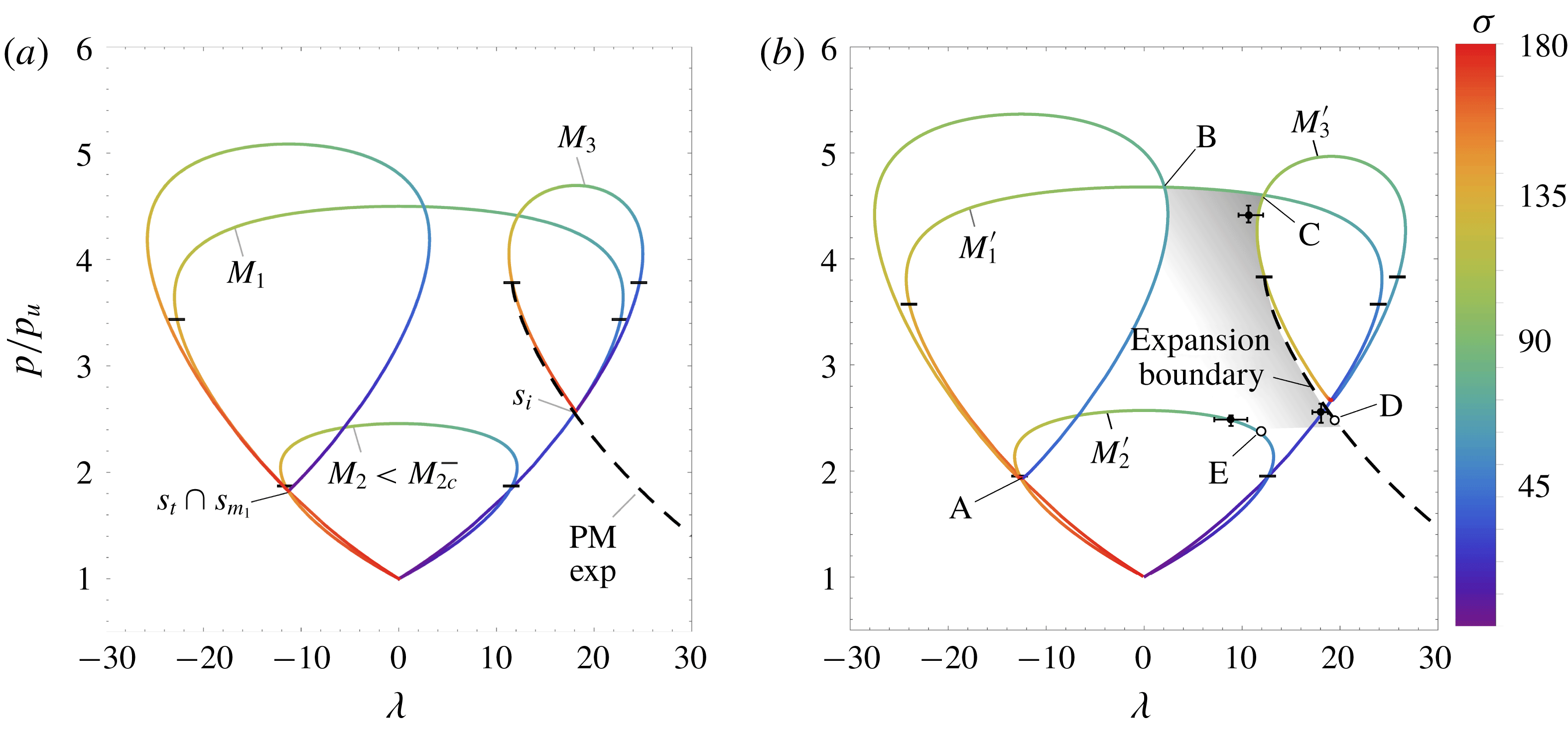
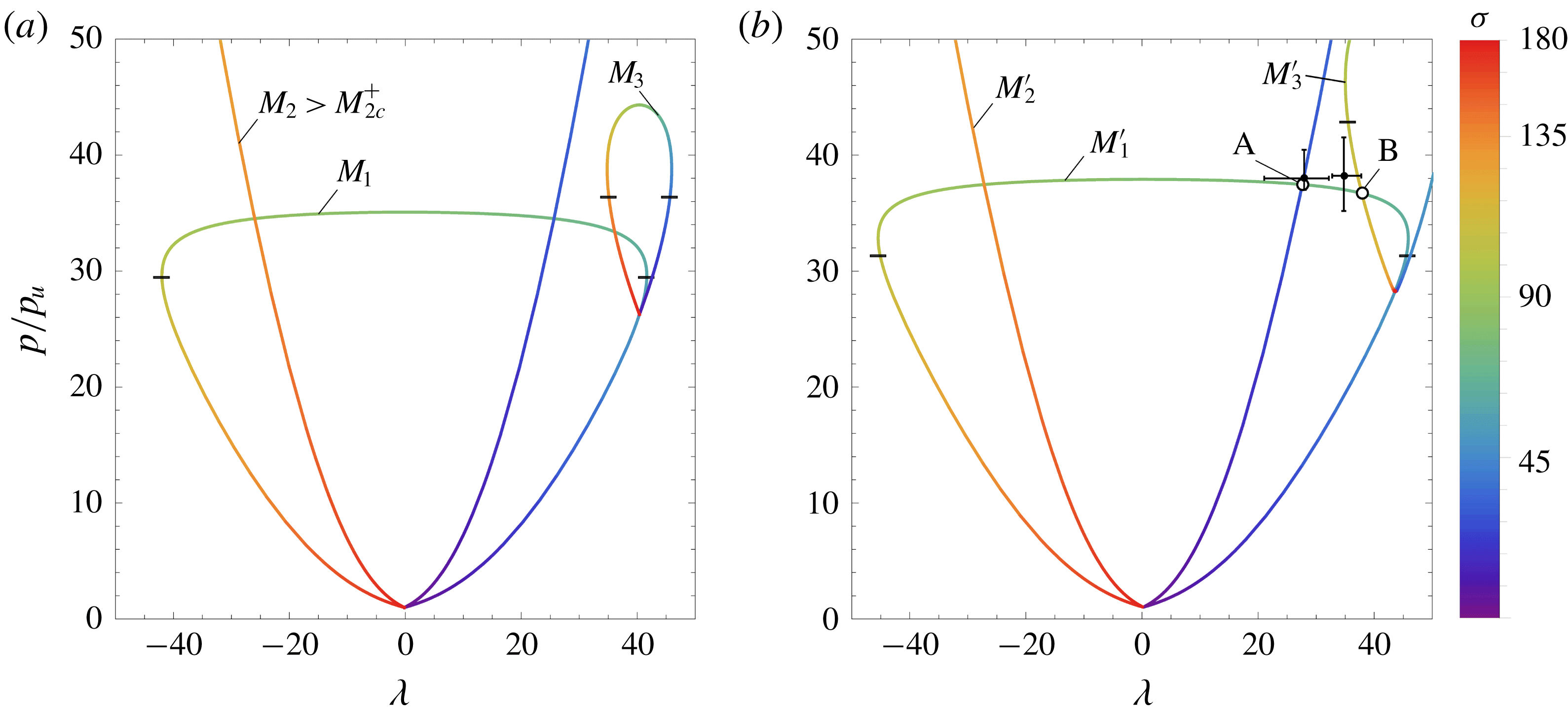
FPR polar plots associated with an oblique shock, with incident angle
 $\unicode[STIX]{x1D70E}_{i}=30^{\circ }$
, crossing an upper stream moving at
 $M_{1}=5$
and lower stream
 $M_{2}=2<M_{2c}^{-}$
. Standard polar plots do not provide a closure to the analytic problem (a), corrected polars given the perturbations
 $\unicode[STIX]{x1D6FF}\unicode[STIX]{x1D6FE}$
and
 $\unicode[STIX]{x1D6FF}M$
for real gases and moving structure (b). Black points denote the numerical solutions evaluated at the different regions with their respective error bars.

FPR simulations showing Mach (a) and pressure field (b) distribution for
 $M_{1}=5$
,
 $M_{2}=2$
and
 $\unicode[STIX]{x1D70E}_{i}=30^{\circ }$
after impingement of the oblique shock with the shear layer.

TNR polar plots for
 $\unicode[STIX]{x1D70E}_{i}=50^{\circ }$
and
 $M_{1}=2$
and
 $M_{2}=1.5<M_{2c}^{-}$
(a), detail of equilibrium solution for real gases and moving structures involving a subsonic region of expansions (shaded area) (b), including the simulation values (black points) with their respective error bars, and analytical solutions (white circles).

The real-gas effects introduced above must be considered to ensure the closure of the problem with the most sensitive process being the expansion wave. In particular, polars widen substantially for small changes in
 $\unicode[STIX]{x1D6FE}$
and more-intense less-deflecting expansions are found. The perturbations to the adiabatic index are computed in the hodograph plane as shown above, varying across the different regions that range from
 $\unicode[STIX]{x1D6FE}_{u}=1.4$
to
 $\unicode[STIX]{x1D6FE}_{B}=1.36$
in the four-shock confluence. Nevertheless, the moving front is also responsible for the final solution. In the moving transmitted-shock reference frame, the incoming flow in the lower stream moves at a higher Mach number
 $M_{2}^{\prime }=M_{2}+\unicode[STIX]{x1D6FF}M_{2}$
, so that pressure downstream is increased up to the value that the interaction demands. As a result of the receding transmitted shock,
 $s_{m_{1}}$
arises to match the static incident shock wave. Consequently, this new shock front must also move with a local inflow Mach number
 $M_{1}^{\prime }=M_{1}+\unicode[STIX]{x1D6FF}M_{1}$
, with
 $\unicode[STIX]{x1D6FF}M_{1}=(a_{2}/a_{1})\unicode[STIX]{x1D6FF}M_{2}$
. When the upper and lower streams share thermodynamical properties, and the sound speeds are equal, the Mach number variation
 $\unicode[STIX]{x1D6FF}M$
is the same in both gas streams. Although the flow behind the incident shock is not affected by the moving structure, the reflected wave does move, varying the pre-shock streamwise Mach number
 $\unicode[STIX]{x1D6FF}M_{3x}=(a_{1}/a_{3})\unicode[STIX]{x1D6FF}M$
and yielding
 $$\begin{eqnarray}\displaystyle \unicode[STIX]{x1D6FF}\unicode[STIX]{x1D706}_{3}=-\text{sin}\,\unicode[STIX]{x1D706}_{3}\frac{\unicode[STIX]{x1D6FF}M_{3x}}{M_{3}}=-\text{sin}\,\unicode[STIX]{x1D706}_{3}\frac{a_{1}}{a_{3}M_{3}}\unicode[STIX]{x1D6FF}M\quad \text{and}\quad \unicode[STIX]{x1D6FF}M_{3}=\cos \unicode[STIX]{x1D706}_{3}\frac{a_{1}}{a_{3}}\unicode[STIX]{x1D6FF}M & & \displaystyle\end{eqnarray}$$
for the flow deflection angle and the total Mach number, respectively. The value of
 $M_{2}^{\prime }$
is then provided by the minimum lower-stream Mach number for which its associated modified polar reaches the final expansion line. This is marked by the tangent solution (C–D) in figure 6(b), where
 $\unicode[STIX]{x1D6FF}M=0.015$
, according to polar-plot theory.
There are some implicit assumptions in the use of the polar-plot method to solve the complex structures mentioned above. One of them is that it resolves the final expansion as a Prandtl–Meyer expansion. Although it is true that this transformation can be taken isentropic within the interaction domain, the assumption that streamlines bend according to (2.9) is not rigorously right because the expansion does not depart from a single point, but rather from a finite region in the non-uniform subsonic flow that radiates pressure changes along Mach lines. Such interaction is far from being trivial, and theoretical descriptions have only been able to cover weak cases. The secondary shock impingement on the transonic shear layer resembles the flow structure analytically studied in Huete et al. (Reference Huete, Urzay, Sánchez and Williams2016), where it was found that the impinging weak shock reflects as a pressure ridge followed by an expansion. Something similar applies to the flow right behind the secondary shock
 $s_{m_{1}}$
, which has been assumed completely homogeneous as the influence from the non-uniform subsonic flow has been neglected. The latter assumption is justified by the linear analysis developed in appendix C, which predicts a very small influence of these pressure waves on
 $s_{m_{1}}$
. As a matter of example, the value of
 $\unicode[STIX]{x1D6E5}_{I}$
computed in figure 20(b) represents the shock trajectory deviations when it is only affected by acoustic waves departing from non-uniform pressure fields
 $\unicode[STIX]{x1D6FF}\unicode[STIX]{x1D70E}=\unicode[STIX]{x1D6E5}_{I}\unicode[STIX]{x1D6FF}p/p$
. For the region of interest behind
 $s_{m_{1}}$
, linear theory predicts
 $\unicode[STIX]{x1D6E5}_{I}\sim 0.2$
, rendering a very small value of the shock trajectory deviation
 $\unicode[STIX]{x1D6FF}\unicode[STIX]{x1D70E}\sim 1.45^{\circ }$
, provided that pressure changes are
 $\unicode[STIX]{x1D6FF}p/p\sim 0.13$
within the influence zone, according to the numerical simulations.
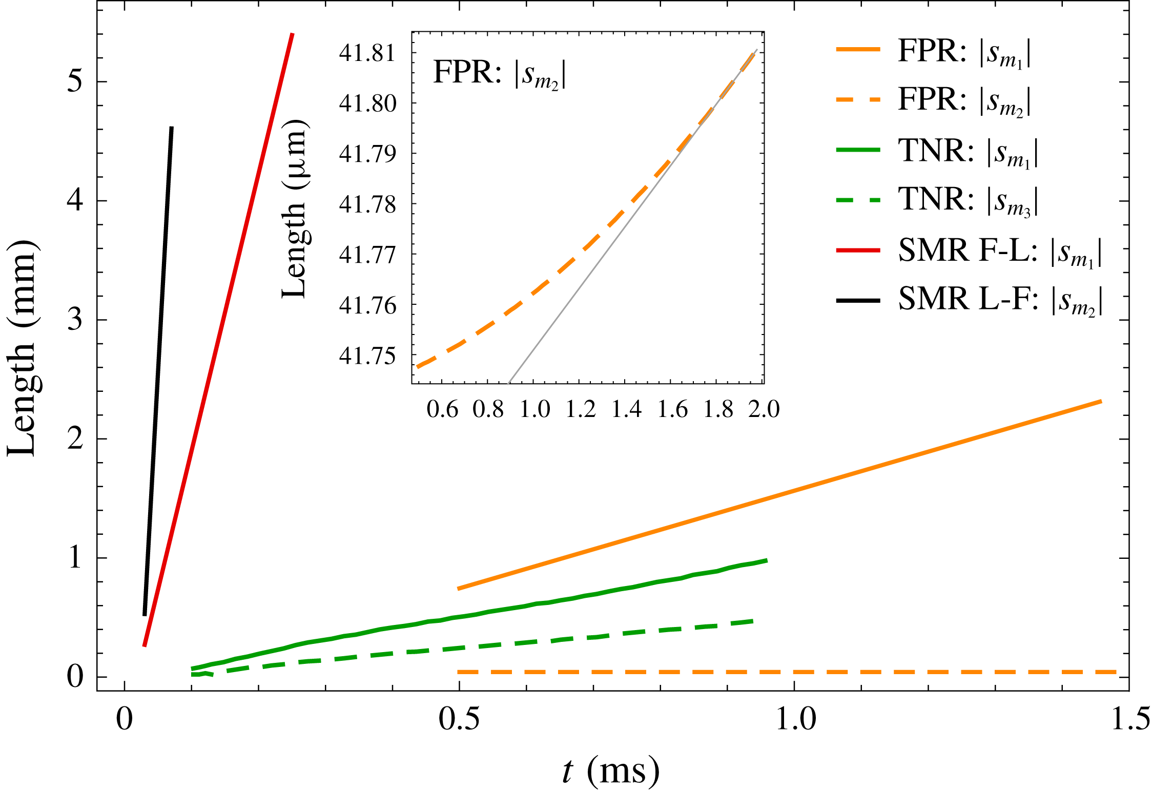
The equilibrium condition predicted by polar plots calls for constant angles of the shock structure, which dictates equal velocities in the backwards-moving intersection points delimiting
 $s_{m_{1}}$
. The structure is pseudosteady when these values remain constant in the polar diagram. In addition, when all the local lengths in the irregular structure grow proportionally in time with the same power law, the flow field is self-similar, akin to those found in shock–wall reflections (Jones et al.
Reference Jones, Martin and Thornhill1951; Sternberg Reference Sternberg1959; Hornung Reference Hornung1986; Tesdall et al.
Reference Tesdall, Sanders and Keyfit2008). Note that, for set-ups made of different gases, such as those carried out by Abd-El-Fattah & Henderson (Reference Abd-El-Fattah and Henderson1978a
,Reference Abd-El-Fattah and Henderson
b
), a modified version of figure 6(b) would apply, with the adjusted Mach numbers providing different equilibrium angles.
The numerical simulation for
 $M_{1}=5$
,
 $M_{2}=2$
and
 $\unicode[STIX]{x1D70E}_{i}=30^{\circ }$
is shown in figure 7, which displays a self-similar solution that is maintained through simulation time. Mach number variations can be used to identify the aforementioned regions of the flow, where the subsonic zone is confined in the dark-brown domain in figure 7(a). The slip line originating at the four-shock confluence is not easily distinguished as the Mach numbers across the shear layer are very similar, although it can be tracked over the streamlines in the right panel. The contact surface, placed at
 $y=0$
, encounters first the backwards-moving transmitted shock, which is curved and generates positive (far bottom-wards) and negative (close to the contact surface) deflection angles. The pressure distribution shown in figure 7(b), behind
 $s_{t}$
and
 $s_{m_{1}}$
, remains nearly uniform
 $p/p_{u}\simeq 5$
as denoted by the equilibrium intersections in figure 6(b). The maximum pressure is placed right behind the four-shock confluence. Although not directly seen because of the wide range in the scale, the subsonic zone is not exactly uniform as deduced from the streamlines deflection in figure 7(b). Spatially averaged values retrieved from the simulations are
 $\langle p_{num}\rangle /p_{u}=5.11$
and
 $\langle p_{num}\rangle /p_{u}=4.27$
for the pressure behind the transmitted shock close to and far below the contact surface, (points A and D, respectively) and
 $\langle p_{num}\rangle /p_{u}=22.3$
for the maximum pressure found behind the four-shock confluence (point B), values in great concordance with the results given by the modified hodograph method. As for the receding velocity, polar-plot theory predicts
 $5.2~\text{m}~\text{s}^{-1}$
, while numerical simulations renders a smaller value,
 $2.1~\text{m}~\text{s}^{-1}$
. This may be explained by the transmitted-shock trajectory, which employs a very long distance in accommodating the equilibrium condition, thereby generating a non-uniform subsonic flow.
4.2 Twin von Neumann reflection (TNR)
The following configuration includes the previously identified secondary shocks of the FPR,
 $s_{m_{1}}$
and
 $s_{m_{2}}$
, plus an extra Mach stem
 $s_{m_{3}}$
that joins the latter to the incident and reflected shocks, as shown in figure 5(b). This forms a kind of symmetric composition of
 $s_{i}$
and
 $s_{r}$
with
 $s_{m_{1}}$
and
 $s_{m_{2}}$
, that gives the name twin von Neumann reflection to this case. This kind of structure arises for weak shocks, although an analogous configuration is possible for strong shocks called twin Mach reflection, TMR, which will not be addressed here.
This distinguished case arises when the reflected and secondary shocks,
 $s_{r}$
and
 $s_{m}$
, do not suffice to provide equilibrium thereby originating an expansion wave in the upper stream, defined previously by their intersection B in figure 6(b). A linking shock
 $s_{m_{3}}$
is produced, defined by the segment of loop between the two intersections B and C shown in figure 8(b), where the Mach stems, the transmitted and the reflected-shock polars are modified in consonance with the relative Mach number
 $\unicode[STIX]{x1D6FF}M=0.02$
and the adiabatic index ranging from
 $\unicode[STIX]{x1D6FE}_{u}=1.4$
to
 $\unicode[STIX]{x1D6FE}_{B}\sim 1.38$
.
TNR simulations showing Mach (a) and pressure field distribution with streamlines (b) for
 $M_{1}=2$
,
 $M_{2}=1.5$
, and
 $\unicode[STIX]{x1D70E}_{i}=50^{\circ }$
after impingement of the oblique shock with the shear layer.

Unlike in the FPR previous case, where the upper stream is supersonic everywhere, the subsonic flow behind the Mach stem impedes solving the local structure by inspection of the polar curves. The subsonic expansion lies in the shaded region of figure 8(b), limited by the known boundaries of the flow, although not explicitly defined by a curve in the hodograph plane, and responsible for the subsonic link of E and D. Note that further increases in
 $\unicode[STIX]{x1D6FF}_{M}$
modifies the stream-2’ polar in the closure direction (displacing E towards D), but also widens stream-1’ polar finally moving away of D, so that no tangential solution is found. Nonetheless, polar plots can still provide useful information for the distinguished zones in the shock-reflection structure, except for its actual dimensions. Perforce, the relative lengths are retrieved from the numerical simulations shown in figure 9, which show that non-uniform regions extend over lengths of greater order of magnitude than the Mach stem length, involving the coupling of the subsonic flow with downstream boundaries. Spatially averaged values retrieved from the simulations are
 $\langle p_{num}\rangle /p_{u}=2.3$
and
 $\langle p_{num}\rangle /p_{u}=4.5$
for points A and D, respectively. Asymptotic far-field pressure values for the end of the expansion and below the transmitted shock are
 $\langle p_{num}\rangle /p_{u}=2.48$
and
 $\langle p_{num}\rangle /p_{u}=2.52$
, respectively. Excluding point A, for which the pressure predicted by theoretical polar plots is lower, the rest of the estimations are definitely consistent with the numerical simulations.
Besides rendering more accurate values, numerical simulations help in providing information about the relative sizes of the secondary shocks, as well as the flow-field properties. From figure 9, a supersonic flow layer separating the subsonic regions formed behind the transmitted shock and the Mach stem is identified. In the absence of boundary constraints, a boundless concave Mach steam would dynamically evolve towards a planar shape, as the downstream mass flux induced parallel to the front would accumulate in the local maximum, pushing the front upwards. The dynamical response could exhibit decaying oscillations until the planar shape is ultimately achieved. In this case, as the Mach stem boundaries are determined by the newly formed triple points, the disequilibrium in the concave Mach stem forces it to move upwards as a whole. For this particular case, however, the value of
 $\unicode[STIX]{x1D6FF}M\sim 0.01$
is found to be quite small.
4.3 Single Mach reflection (SMR)
4.3.1 Fast–slow SMR
We shall now consider the flow structure shown in figure 5(c), which appears, e.g. for
 $M_{1}=5$
,
 $\unicode[STIX]{x1D70E}_{i}=60^{\circ }$
and
 $M_{2}=4<M_{2c}^{-}$
. There, a new shear layer is recognized between subsonic and supersonic regions arising from the triple point, namely the confluence of the incident, reflected and Mach stem shocks. Analogously to solutions of FPR type, when
 $M_{2}$
is reduced below the critical value
 $M_{2c}^{-}$
, regular configurations fail to provide downstream equilibrium as shown in figure 10(a), with the overpressure triggering the evolution of quasi-steady structures. Akin to the previous case, the Mach stem curvature impedes static equilibrium so it moves upwards, along with the transmitted shock, causing an increase of the relative Mach number.
Fast–slow SMR regular polar plot for
 $\unicode[STIX]{x1D70E}_{i}=60^{\circ }$
,
 $M_{1}=5$
and
 $M_{2}=4$
(a), detail of corrected equilibrium solution involving a subsonic region of expansions (shaded area) (b) with measured values from the simulations (black points), and analytical solutions (white circles).

Fast–slow SMR simulations showing Mach (a) and pressure field distribution with streamlines (b) for
 $M_{1}=5$
,
 $M_{2}=4$
and
 $\unicode[STIX]{x1D70E}_{i}=60^{\circ }$
.

The complete polars are presented in figure 10(b), where the subsonic flow with the appropriate expansion is shown in a shaded area as in the TNR, with
 $\unicode[STIX]{x1D6FF}M\sim 0.1$
and adiabatic index ranging from
 $\unicode[STIX]{x1D6FE}_{u}=1.4$
to
 $\unicode[STIX]{x1D6FE}_{B}=1.33$
, measured at the moving shocks in the numerical solution. The properties of the Mach stem are given by the
 $M_{1}^{\prime }$
curve and predict a positive angle for
 $\unicode[STIX]{x1D70E}_{m}$
in contact with
 $s_{i}$
and negative with
 $s_{t}$
as recovered from the simulations, see figure 11. Intersection A of stream-1’ and stream-2’ polars yields the conditions at the impingement of the shock with the shear layer, which provides the local angle of the shocks at each side, rendering subsonic and supersonic flow in the lower and upper stream, respectively. The upper conditions form a small supersonic patch that originates a new slip line in contact with the Mach stem, siting very close to the original slip line of the shear layer. This seems a degenerate version of the previous TNR case, where the supersonic intermediate layer becomes a point with no scale linking the regions.
In turn, the span of the secondary wave that generates the supersonic pocket remains negligible to the progressively growing Mach stem, thus sets the slip lines close together enclosing supersonic post-shock conditions at the confluence point in
 $y=0$
, see A–B. Consideration of viscous and thermal effects would provide a proper development scale to which these small structures could be compared.
The flow behind the reflected shock is supersonic, with higher pressure than the region behind the transmitted shock. Although it is not noticeable from the framework displayed in figure 11, a closer look at the triple-shock point C reveals a Guderley-type locus, with a well-delimited subsonic patch appearing akin to that predicted by Vasilev, Elperin & Ben-Dor (Reference Vasilev, Elperin and Ben-Dor2008). Such non-idealized flow patterns, whose characteristic length is much smaller than large-scale structures developed in the pseudosteady regime, have been experimentally observed in shock–wall reflection phenomena (Skews & Ashworth Reference Skews and Ashworth2005; Skews, Li & Platon Reference Skews, Li and Platon2009) and have been now found in irregular interactions with contact surfaces. Since this work mainly focuses on the large-scale structures, a thorough analysis on this small-scale formation is not provided in this work. Roughly, the fluid particle departs from the triple shock and crosses the small subsonic patch while expanding isentropically, with a flow deflection function that can be approximated with a Prandtl–Meyer expansion, as observed in the numerical simulations.
Finally, note that the transmitted shock displays a varying angle along the
 $M_{2}^{\prime }$
curve from the interaction with
 $M_{1}^{\prime }$
to the value given at equilibrium pressure. Far-field numerical solution shows that pressure equilibrium is not achieved between the upper expansion and the flow right behind the transmitted shock far below the contact surface, such as the region in between (left out in figure 11 for clarity purposes), is not uniform. This is mainly due to the strong pressure and deflection-angle gradients found in the intersection point, which induce strong vortex structures convected downwards. Here, the values predicted by the modified polars are
 $\unicode[STIX]{x1D70E}_{t}(y=0)=105.1^{\circ }$
, referring to the transmitted shock very close to the contact surface, and
 $\unicode[STIX]{x1D70E}_{r}=157.6^{\circ }$
for the reflected shock departing from the triple point. The corresponding pressure values are
 $p/p_{u}\simeq 30$
and
 $p_{5}/p_{u}\simeq 19$
, whose comparison with numerical simulations stands in good agreement for
 $\langle p_{num}\rangle /p_{u}=29.51$
and
 $\langle p_{num}\rangle /p_{u}=19.05$
. However, the gap between the deflection angles provided by D and E in the polar plots is connected via the subsonic vortex sheet with varying deflection angle that is formed at the slip lines. As expected, the supersonic upper region that is less affected by the non-uniform subsonic zone, is reproduced by the polar plots with higher accuracy.
4.3.2 Slow–fast SMR
An irregular flow-field configuration of the SMR kind is also observed when the lower edge supersonic Mach number exceeds a critical value, out of the weak-shock limit. This critical value is easily found in figure 2(b) at the curve bending in the right side of the plot. Beyond this value, there is no solution of the regular kind. The case illustrated in figure 12(a) represents the standard polar plots for critical conditions
 $M_{1}=5.5$
,
 $\unicode[STIX]{x1D70E}_{i}=60^{\circ }$
,
 $M_{2}>M_{2c}^{+}$
. It is readily seen that for
 $M_{2}>M_{2c}^{+}$
the polar for
 $M_{2}$
no longer intersects the polar
 $M_{3}$
of the reflected shock, arising from the incident-shock conditions. The resulting configuration is computed in figure 12(b) considering the value of
 $\unicode[STIX]{x1D6FF}M\sim 0.1$
for the upstream moving structure, according to the simulations, and the effects on
 $\unicode[STIX]{x1D6FE}$
. A clear picture of the intersection is given by the numerical simulations shown in figure 13. The Mach stem connecting
 $M_{1}^{\prime }$
–
 $M_{2}^{\prime }$
and
 $M_{1}^{\prime }$
–
 $M_{3}^{\prime }$
crossing points is easily identified, thereby generating a new slip line in the downstream flow. The flow in zones A and B departs with different angles,
 $\unicode[STIX]{x1D706}_{B}>\unicode[STIX]{x1D706}_{A}$
, which forces the acceleration of the subsonic fluid particles along the stream lines.
Slow–fast SMR polar plots associated with an oblique shock, with incident angle
 $\unicode[STIX]{x1D70E}_{i}=60^{\circ }$
, crossing an upper stream moving at
 $M_{1}=5.5$
and a lower stream
 $M_{2}=10$
(a). Corrected polars including numerical solution measurements (black points) (b).

Slow–fast SMR simulations showing Mach and pressure field distribution for
 $M_{1}=5.5$
,
 $M_{2}=10$
and
 $\unicode[STIX]{x1D70E}_{i}=60^{\circ }$
.

This irregular configuration demands high Mach streams that translate into high pressures downstream. Consequently, temperature changes are alike, with the associated real-gas effects taking a dominant role in providing the equilibrium conditions. As a matter of example, the value of
 $\unicode[STIX]{x1D6FE}$
in points A and B reaches
 $\unicode[STIX]{x1D6FE}\sim 1.32$
. The corresponding pressure values of the polar plots are
 $p/p_{u}\simeq 38$
and
 $p/p_{u}\simeq 37$
for points A and B, respectively, and indicate a good correspondence with the numerical simulations. They are
 $\langle p_{num}\rangle /p_{u}=38.24$
and
 $\langle p_{num}\rangle /p_{u}=37.92$
for the pressure at the contact point A and right behind the triple point B, respectively. According to figure 12(a), calorically perfect predictions yield significantly smaller values of pressure. From figure 12 it is also evidenced that critical conditions are affected by the
 $\unicode[STIX]{x1D6FE}$
value reduction. In particular, as the polar plots widens with temperature, the value of
 $M_{2c}^{+}$
is found to be greater and the regular reflection domain broadens. For instance,
 $M_{1}=5$
,
 $\unicode[STIX]{x1D70E}_{i}=60^{\circ }$
and
 $\unicode[STIX]{x1D6FE}(T)$
render
 $M_{2c}^{+}=8.1$
, which is definitely greater than
 $M_{2c}^{+}=7.29$
computed in table 1 for
 $\unicode[STIX]{x1D6FE}=1.4=\text{constant}$
.
5 Discussion
5.1 Self-similar regime
Relevant studies on irregular configurations arising at the interaction with a gas interface have been instrumental in providing deeper understanding of this topic through intricate experimental methods (Abd-El-Fattah & Henderson Reference Abd-El-Fattah and Henderson1978b
). There, a shock produced in a tube for different pressure-jump intensities interacts with a contact surface between two gases at rest, generating reflected structures on a layer of non-zero convective Mach number from a fixed-reference view point. Even though their results on a gas interface of constant properties are captured via numerical simulations, accounting for possible shear or temperature differences, such that
 $M_{1}\neq M_{2}$
, calls for more subtle details to be addressed. Here, proper consideration of a moving reference frame with the incident shock allows us to identify the nature of the final structure that grows as the transmitted shock further moves against the stream. This explains the lack of agreement between the experimental and theoretical results for increasing shock intensities. The modified speed that we introduced above, obtained from numerical data, provides equilibrium conditions in the hodograph plane with a reasonable degree of accuracy. This is valid when the upper stream is supersonic everywhere and leads to conditions that are uneasy to comprehend for a passing shock on their laboratory-fixed reference frame. There, some confusion was shed under the unavoidable transient effects and wall reflections of the experiments, which yield in particular the bound precursor reflection (BPR) type of interaction that we have been unable to find in the open domain. Furthermore, in the free precursor type (FPR) and twin von Neumann refraction (TNR) the transmitted waves were said to propagate faster than the incident shock, which complicated the harmonization with their self-similar observations.
Here,
 $M_{2}<M_{2c}^{-}$
cases have shed light into their pseudosteady nature, with the self-similar structure displacing as a whole with the speed that yields the minimum pressure increase needed to render downstream equilibrium. As noted above, the intersection of the PM curve, which represents the expansion of the fluid particles behind the origin of the reflected shock, with the modified polar plot for the lower stream, given by the Mach number measured from the counter-stream moving transmitted shock, provides the final equilibrium conditions. As the departure conditions of the final PM-expansion depend on the relative upstream Mach number, the equilibrium point must be resolved iteratively. Fortunately, since the reflected shock is not very strong, the final Prandtl–Meyer expansion renders conditions that are very similar to those obtained with the reflected expansion in regular interactions. Therefore, the relative Mach number of the transmitted shock with respect to the incoming stream scales with the deviation from critical conditions
 $\unicode[STIX]{x1D6FF}M\sim M_{2}^{\prime }-M_{2c}^{-}$
.
Second, the case
 $M_{2}>M_{2c}^{+}$
, computed in figure 13, shows a seemingly simple structure with the reflected and transmitted shock plus a Mach stem, whose formation is predicted by polar plots. The length of this Mach stem, or those found in figures 7 and 11, cannot be predicted by the length-less equations employed in the polar diagrams. The moving transmitted shock together with the anchored incident shock, relate the length of the Mach stem to the retreating velocity and the evolution time. This fact indicates that information about the largest length scale involved in the problem, being the domain length scale, must eventually reach the Mach stem (Hornung Reference Hornung1986). This clearly occurs through the downstream flow behind the Mach stem that is inherently subsonic. Nonetheless, the length of this Mach stem has been found to play a negligible role in predicting the properties of the backwards-travelling transmitted wave. It is suggested that constraints in the boundary domains, such as the walls in the experiments conducted by Abd-El-Fattah & Henderson (Reference Abd-El-Fattah and Henderson1978a
), can make the Mach stem length growth saturate at increasing times.
The numerical method employed, in consonance with the theory used in computing the polar diagrams, is set to the inviscid Euler equations, so that the only length scale involved in the problem enters through the domain size. The shear layer only diffuses via numerical effects, which have been observed to be negligible within the local interaction structure domain. For instance, some shocks are much shorter than other lengths appearing in the irregular structure as seen in figure 11 for the subsonic pocket, which in the absence of viscous effects adapts to the minimum mesh size. The consideration of viscosity will provide additional scales to compare with, being the mixing-layer thickness the most important one at early times. This will affect the post-shock conditions if these small structures that have lead to nearly discontinuous solutions. In turn, if the shear layer becomes turbulent, the numerical method calls for realistic three-dimensional computations that resolve all contributions of the vorticity perturbations, which would include additional scales. However, this is out of the scope of the present work and it is left for future studies.
Distance between Mach stem boundaries as a function of time for FPR, TNR, SMR structures.

It must be also stated that, as a result of the high nonlinearity of the problem, the final flow–structure configuration depends on the initial conditions. For the cases considered here, where the flow is initiated with the two coflowing streams and the shock originated at the corner imposed by the flow deflection, the asymptotic structure is found to settle at short times after the shock impingement in the tangential discontinuity. Afterwards, although it moves and expands in the physical domain, the structure becomes self-similar as all the angles remain unaltered. This finding was explained by the permanence of the intersection points in the polar plots.
A relatively simple demonstration is provided in figure 14, which shows the length of the secondary shocks that appear in the irregular reflections. If the secondary shocks’ length grows proportional to time, the Euler equations can be rewritten in a self-similar form through the transformation
 $\tilde{x}=x/t$
,
 ${\tilde{y}}=y/t$
, as the analysis performed by Sternberg (Reference Sternberg1959), Samtaney (Reference Samtaney1997) for Mach–wall reflections. It is seen that shortest lengths, as is
 $|s_{m_{2}}|$
in the FPR structure, takes longer to fit into the linear trend, as its length is comparable to the shear-layer thickness at early times.
5.2 Induced vorticity downstream
The vorticity amplification that the contact surface experiences across the oblique shock, which depends on the velocity (shear type) and density (baroclinic source) jumps, is of paramount importance in supersonic propulsion devices (Urzay Reference Urzay2018). There, shocks generated in the air stream at wedged walls and fuel injectors impinge on the shear layer surrounding the fuel jets downstream from the injection point (Laurence et al. Reference Laurence, Karl, Schramm, Martínez and Hannemann2013). Although the flow is typically turbulent in these high Reynolds number applications, analyses of laminar flows have been shown to be instrumental in providing insightful information pertaining to mixing augmentation by vorticity production as studied by Menon (Reference Menon1989), Lu & Wu (Reference Lu and Wu1991), Gutmark, Schado & Yu (Reference Gutmark, Schado and Yu1995), Buttsworth (Reference Buttsworth1996) and Tritarelli & Kleiser (Reference Tritarelli and Kleiser2017), and enhanced chemical reaction leading to ignition behind the curved shock in recent works (Huete et al. Reference Huete, Sánchez, Williams and Urzay2015; Huete, Sánchez & Williams Reference Huete, Sánchez and Williams2017). The acoustic coupling in the shock train has been observed to experience unsteady responses, even for simple geometrical configurations (Xiong, Wang & Tao Reference Xiong, Wang and Tao2018). More realistic configurations would involve the presence of multi-gas flow field, with the spatially evolving mixing and shear layers having a significant impact on the final shock-train structure. The characterization of the limits below which the shock transmission/reflection remains steady, as well as the eventual evolution of unsteady shock configurations is crucial in the design of supersonic combustion chambers.
The interaction of the oblique shock with perturbed shear layer triggers the unstable growth of the contact surface ripple, which can be seen as a combination of Kelvin–Helmholtz and Richtmyer–Meshkov instabilities (Samtaney & Zabusky Reference Samtaney and Zabusky1993; Mikaelian Reference Mikaelian1994; Rikanati et al.
Reference Rikanati, Sadot, Ben-Dor, Shvarts, Kuribayashi and Takayama2006; Rubidge & Skews Reference Rubidge and Skews2014). In this respect, the analysis of the perturbations growth behind the shock impingement cannot be uniquely determined by the free-stream Mach numbers
 $M_{2}-M_{1}$
, as the upstream shear
 $(U_{2}-U_{1})/\unicode[STIX]{x1D6FF}_{u}$
and the density
 $\unicode[STIX]{x1D70C}_{2}-\unicode[STIX]{x1D70C}_{1}$
would contribute differently. The latter is the baroclinic contribution, as there are unaligned density and pressure gradients across the shock impingement. It has been previously reported that considering lighter gases in the low-speed stream, which is an archetype configuration of hydrogen–air mixing layers in scramjets, makes the two contributions have a destructive interference.
An example of the large-scale vorticity structures generated at the shock is provided in figure 15 for the fast–slow SMR simulation. The initial vorticity associated with the coflowing streams, namely
 $(U_{1}-U_{2})/\unicode[STIX]{x1D6FF}_{u}$
, is amplified by the shock impingement. The downstream vorticity sheet rolls up, thereby generating local eddies that propagate downstream convected by the fluid particles. This effect will promote the macroscopic mixing of the compressed gases. Clearly, viscosity will have a pivotal effect in the mixing rate, as the vorticity distribution will be dominated by viscous effects at scales of the order of
 ${\sim}\unicode[STIX]{x1D6FF}_{u}$
. A detailed study of the expected mixing enhancement induced by the oblique-shock impingement (Menon Reference Menon1989; Lu & Wu Reference Lu and Wu1991; Gutmark et al.
Reference Gutmark, Schado and Yu1995) would require the resolution of the mixing-layer region, with the upstream turbulent fluctuations demanding three-dimensional computations (Martínez-Ferrer, Lehnasch & Mura Reference Martínez-Ferrer, Lehnasch and Mura2017; Fang et al.
Reference Fang, Shen, Sun and Hu2018; Rao et al.
Reference Rao, Asano, Imani and Saito2018). However, such detailed analysis would exceed the scope of the present paper.
Dimensionless vorticity field, scaled with the upstream shear
 $(U_{1}-U_{2})/\unicode[STIX]{x1D6FF}_{u}$
, for the fast–slow SMR simulation:
 $M_{1}=5$
,
 $M_{2}=4$
and
 $\unicode[STIX]{x1D70E}_{i}=60^{\circ }$
.

6 Concluding remarks
The response of shock waves impinging on contact surfaces, mixing or shear layers, has been addressed here to obtain further understanding on compressible-flow irregular configurations in semi-infinite domains. The critical conditions of convective Mach number and incident shock angle under which these structures arise are delineated from a theoretical zero-dimensional analysis of the inviscid regular problem. These limits to regular solutions are further studied by means of the hodograph plane and high-fidelity numerical simulations of inviscid flows.
In this work, classic polar plots have been extended to include real-gas effects and the effective Mach number at the retreating shocks to be applied to the atlas of irregular configurations. It has been found that the moving set of waves is a result of the lack of mechanical balance in regular configurations, which pushes back the set increasing the relative Mach number and favours the achievement of downstream balanced conditions. Therefore, once the stable conditions are reached, the angles that form the asymptotically growing structure remain unaltered and produce self-similar solutions.
The modified hodograph method provides, with an acceptable degree of accuracy, values of the distinguished complex configurations. In particular, it reproduces remarkably well combined details such as triple shocks, local intersections, shock confluences and expansions. By way of contrast, diagrams do not provide any information about the characteristic size of the structure, which remains a function of time. Nevertheless, the scale of the domain must arise at large times, as it is the only typical length involved and it determines the final stages of the structure.
Numerical simulations using the inviscid Euler equations have been used here to characterize the irregular configurations removing the viscous–diffusive length scale of the problem. This removes the Reynolds number dependency or the classical length scale given as the distance of the impingement to the origin of the mixing layer. These simulations enable the visualization of the complex shock structures, and are able to provide the growth rate of the shock lengths. In addition, they have also been instrumental in confirming the spurious character of particular cases, such as the unstable upper-branch solutions of regular configurations, and discarding them.
From the far-field standpoint, when a single reflected wave cannot yield conditions to provide equilibrium downstream, two mayor events can happen. For fast–slow shear layers, as the transmitted shock pressure is not sufficiently high, the generation of a reflected shock is accompanied with a posterior expansion, and the transmitted shock retreats as a consequence of the pressure mismatch. As a result, secondary shocks must come into play to join the moving transmission and the fixed impinging shock. In this regard, the upper stream and the incoming wave govern the final flow configuration. For slow–fast shear layers, the far-field qualitative picture is similar, but with the absence of the expansion flow downstream since the transmitted shock pressure is higher than that demanded by the mechanical equilibrium in static conditions. In both scenarios, the local structure defined by finite-length shocks are formed in the upper-stream layer.
Acknowledgements
The work of D.M.R. and C.H. was supported by grants ENE2015-65852-C2-1-R (MINECO/FEDER, UE) and BYNV-ua37crdy (Fundación Iberdrola España). Numerical simulations were performed at Altamira Supercomputer thanks to the grant FI-2017-3-0041 (RES). D.M. acknowledges the Juan de la Cierva postdoctoral grant with code IJCI-2015-2668. The authors gratefully acknowledge Dr A. Mura, CNRS researcher at Institut PPRIME in France, for the numerical tool CREAMS.
Appendix A. Details of numerical simulations
The unsteady, three-dimensional, compressible Euler equations of a multi-species thermally perfect-gas mixture, namely
 $$\begin{eqnarray}\displaystyle & \displaystyle \frac{\unicode[STIX]{x2202}^{}\unicode[STIX]{x1D70C}}{\unicode[STIX]{x2202}t^{}}+\frac{\unicode[STIX]{x2202}^{}\unicode[STIX]{x1D70C}u_{j}}{\unicode[STIX]{x2202}{x_{j}}^{}}=0, & \displaystyle\end{eqnarray}$$
 $$\begin{eqnarray}\displaystyle & \displaystyle \frac{\unicode[STIX]{x2202}^{}\unicode[STIX]{x1D70C}u_{i}}{\unicode[STIX]{x2202}t^{}}+\frac{\unicode[STIX]{x2202}^{}\unicode[STIX]{x1D70C}u_{i}u_{j}}{\unicode[STIX]{x2202}{x_{j}}^{}}+\frac{\unicode[STIX]{x2202}^{}p}{\unicode[STIX]{x2202}{x_{i}}^{}}=0,\quad i=1,2,3, & \displaystyle\end{eqnarray}$$
 $$\begin{eqnarray}\displaystyle & \displaystyle \frac{\unicode[STIX]{x2202}^{}\unicode[STIX]{x1D70C}e_{t}}{\unicode[STIX]{x2202}t^{}}+\frac{\unicode[STIX]{x2202}^{}(\unicode[STIX]{x1D70C}e_{t}+p)u_{j}}{\unicode[STIX]{x2202}{x_{j}}^{}}=0, & \displaystyle\end{eqnarray}$$
 $$\begin{eqnarray}\displaystyle & \displaystyle \frac{\unicode[STIX]{x2202}^{}\unicode[STIX]{x1D70C}Y_{\unicode[STIX]{x1D6FC}}}{\unicode[STIX]{x2202}t^{}}+\frac{\unicode[STIX]{x2202}^{}\unicode[STIX]{x1D70C}Y_{\unicode[STIX]{x1D6FC}}u_{j}}{\unicode[STIX]{x2202}{x_{j}}^{}}=0,\quad \unicode[STIX]{x1D6FC}=1,\ldots ,N, & \displaystyle\end{eqnarray}$$
are numerically solved for the spatially developing shear layers studied in this work. In the above system,
 $t$
denotes the time,
 $x$
is the Cartesian coordinate with subscripts
 $i$
and
 $j$
referring to spatial directions,
 $u_{i}$
is the velocity component in
 $i$
-direction,
 $\unicode[STIX]{x1D70C}$
is the density,
 $p$
is the pressure,
 $e_{t}=e+u_{i}u_{i}/2$
is the total specific energy (obtained from the internal specific energy,
 $e=h-p/\unicode[STIX]{x1D70C}$
, and the kinetic energy) and
 $Y_{\unicode[STIX]{x1D6FC}}$
is the mass fraction of species
 $\unicode[STIX]{x1D6FC}$
, being
 $N$
the total number of species in the mixture. Thermodynamic variables follow the equation of state of an ideal-gas mixture,
 $p=\unicode[STIX]{x1D70C}RT/W$
, where
 $R=8.314~\text{J}~\text{mol}^{-1}~\text{K}$
is the universal gas constant and
 $T$
and
 $W(\unicode[STIX]{x1D6FC})=(\sum _{\unicode[STIX]{x1D6FC}=1}^{N}Y_{\unicode[STIX]{x1D6FC}}/W_{\unicode[STIX]{x1D6FC}})^{-1}$
are the temperature and molar mass of the gas mixture, respectively. The enthalpy,
 $h(\unicode[STIX]{x1D6FC},T)=\sum _{\unicode[STIX]{x1D6FC}=1}^{N}h_{\unicode[STIX]{x1D6FC}}(T)$
, and heat capacity,
 $c_{p}(\unicode[STIX]{x1D6FC},T)=\sum _{\unicode[STIX]{x1D6FC}=1}^{N}c_{p,\unicode[STIX]{x1D6FC}}(T)$
, are functions of the temperature and mixture composition (calculated via JANAF tables, see Stull & Prophet (Reference Stull and Prophet1971)). Therefore, the ratio of specific heats
 $\unicode[STIX]{x1D6FE}=c_{p}/c_{v}$
is not constant. For same-gas shear layers, like the ones studied in this work, the value of
 $\unicode[STIX]{x1D6FE}$
is uniquely determined by the temperature.
The numerical simulation of compressible flows does require the use of highly accurate numerical schemes capable of capturing shock waves precisely. Consequently, the spatial discretization of the first-order derivatives in (A 1)–(A 4) is carried out with a seventh-order accurate hybrid upwinded-WENO scheme (see Balsara & Shu (Reference Balsara and Shu2000) for a detailed description of the WENO implementation), whilst time integration is performed via a third-order, total variation diminishing, Runge–Kutta scheme as described by Gottlieb & Shu (Reference Gottlieb and Shu1998). The aforementioned equations and numerical procedures are integrated in the direct numerical simulation (DNS) solver CREAMS, which has been thoroughly described and validated in a previous work (Martínez-Ferrer et al. Reference Martínez-Ferrer, Buttay, Lehnasch and Mura2014).
Following previous works based on temporally developing (Pantano & Sarkar Reference Pantano and Sarkar2002; Mahle et al. Reference Mahle, Foysi, Sarkar and Friedrich2007) and spatially developing (Stanley & Sarkar Reference Stanley and Sarkar1997; Fu & Li Reference Fu and Li2006; Martínez-Ferrer et al. Reference Martínez-Ferrer, Lehnasch and Mura2017) shear layers, the flow is initialized using a hyperbolic tangent profile for the mean streamwise component of the velocity
 $$\begin{eqnarray}\displaystyle u_{1}=\frac{U_{1}+U_{2}}{2}+\frac{U_{1}-U_{2}}{2}\tanh \left(\frac{2y}{\unicode[STIX]{x1D6FF}_{\unicode[STIX]{x1D714},0}}\right), & & \displaystyle\end{eqnarray}$$
whilst the other two orthogonal components are set to zero. In (A 5),
 $U_{1}$
and
 $U_{2}$
are the mean streamwise velocities of the top and bottom streams, respectively,
 $\unicode[STIX]{x1D6FF}_{\unicode[STIX]{x1D714},0}\equiv \unicode[STIX]{x1D6FF}_{\unicode[STIX]{x1D714}}(x=0)=(U_{1}-U_{2})/(|\unicode[STIX]{x2202}\langle u_{1}\rangle _{f}/\unicode[STIX]{x2202}x_{2}|_{\max ,0})$
is the initial vorticity thickness of the shear layer where brackets indicate Reynolds averaged quantities, with the additional index
 $f$
utilized for Favre averaged quantities. The thermodynamic conditions of all the shear layers studied in this work correspond indeed to the ICAO standard atmosphere (
 $p=101325~\text{Pa}$
and
 $T=288.15~\text{K}$
) and the retained air mixture composition is given by
 $X_{O_{2}}=0.21$
and
 $X_{N_{2}}=0.79$
for the volume fractions of hydrogen (
 $\unicode[STIX]{x1D6FC}=1$
) and nitrogen (
 $\unicode[STIX]{x1D6FC}=2$
) species, respectively.
In (A 5), the initial vorticity thickness is a crucial parameter defining the problem because it controls the amount of initial diffusion between the two streams of the shear layer. This quantity has an associated Reynolds number
 $$\begin{eqnarray}\displaystyle Re_{\unicode[STIX]{x1D714},0}=\frac{\bar{\unicode[STIX]{x1D70C}}\unicode[STIX]{x0394}U\unicode[STIX]{x1D6FF}_{\unicode[STIX]{x1D714},0}}{\bar{\unicode[STIX]{x1D707}}}, & & \displaystyle\end{eqnarray}$$
where
 $\unicode[STIX]{x0394}U=|U_{1}-U_{2}|$
,
 $\bar{\unicode[STIX]{x1D70C}}=(\unicode[STIX]{x1D70C}_{1}+\unicode[STIX]{x1D70C}_{2})/2$
and
 $\bar{\unicode[STIX]{x1D707}}=(\unicode[STIX]{x1D707}_{1}+\unicode[STIX]{x1D707}_{2})/2$
. Following the literature of supersonic inert mixing layers (Pantano & Sarkar Reference Pantano and Sarkar2002; Fu & Li Reference Fu and Li2006; Martínez-Ferrer et al.
Reference Martínez-Ferrer, Lehnasch and Mura2017), the value
 $Re_{\unicode[STIX]{x1D714},0}=640$
is retained in the present work. With this value one can deduce from (A 6) the initial vorticity thickness of a given shear layer and thus its corresponding velocity profile with (A 5). The grid size employed in numerical simulations is a factor of the initial vorticity thickness
 $\unicode[STIX]{x1D6FF}_{\unicode[STIX]{x1D714},0}=2.8\times 10^{-5}~\text{m}$
, and has a typical value corresponding to DNS of
 $\unicode[STIX]{x0394}x\approx 0.168\unicode[STIX]{x1D6FF}_{\unicode[STIX]{x1D714},0}$
according to the literature (Pantano & Sarkar Reference Pantano and Sarkar2002; Mahle et al.
Reference Mahle, Foysi, Sarkar and Friedrich2007; Martínez-Ferrer et al.
Reference Martínez-Ferrer, Lehnasch and Mura2017). Clearly, the definition of the vorticity thickness is not compatible with the system of Euler equations describing the shear layers of this work, since the hyperbolic tangent profile (A 5) would asymptotically degenerate into a step function as
 $\unicode[STIX]{x1D6FF}_{\unicode[STIX]{x1D714},0}=0$
for an inviscid flow. However,
 $\unicode[STIX]{x1D6FF}_{\unicode[STIX]{x1D714},0}\neq 0$
is employed for the following two reasons: (i) it provides an estimated grid size for the numerical simulations and (ii) it allows for comparing results with the vast majority of previous works based on that definition. A parametric study is conducted below to assess the difference between
 $\unicode[STIX]{x1D6FF}_{\unicode[STIX]{x1D714},0}=0$
and
 $\unicode[STIX]{x1D6FF}_{\unicode[STIX]{x1D714},0}\neq 0$
approaches.
A rectangular computational domain, measuring
 ${\sim}600\,\unicode[STIX]{x1D6FF}_{\unicode[STIX]{x1D714},0}\times 600\,\unicode[STIX]{x1D6FF}_{\unicode[STIX]{x1D714},0}$
, is employed, where is the initial vorticity thickness that acts as the numerical reference length in this problem. The area of interest where the two streams are defined (see figure 1) covers a squared region of dimensions
 $100\,\unicode[STIX]{x1D6FF}_{\unicode[STIX]{x1D714},0}\times 100\,\unicode[STIX]{x1D6FF}_{\unicode[STIX]{x1D714},0}$
, placed at the top left corner of the entire domain. This area features a constant grid size of
 $\unicode[STIX]{x0394}x=0.25\,\unicode[STIX]{x1D6FF}_{\unicode[STIX]{x1D714},0}$
whilst the rest of the computational domain is linearly stretched towards the boundaries with a constant factor of 5 %. Boundary conditions are implemented as follows: the left boundary acts as a supersonic inlet where Dirichlet conditions are imposed for pressure, temperature and mixture composition (ICAO standard atmosphere) whilst the velocity profile follows (A 5) where
 $U_{2}$
changes over time. At the top boundary generalized Rankine–Hugoniot jump conditions for an ideal-gas mixture are applied (Martínez-Ferrer et al.
Reference Martínez-Ferrer, Buttay, Lehnasch and Mura2014) and non-reflecting boundary conditions are specified at the bottom and right boundary conditions. A constant value of 0.5 for the Courant–Friedrichs–Lewy (CFL) condition is specified to advance the simulation in time.
For the sake of simplicity and computational-cost efficiency, the following assumptions have been made in the present work. Simulation sets are run as follows: First, the upper-stream Mach number
 $M_{1}$
remains fixed whilst the bottom stream is either accelerated (
 $M_{1}\leqslant M_{2}$
) or decelerated (
 $M_{1}\geqslant M_{2}$
) from an initial value of
 $M_{2}=M_{1}$
. Second, instantaneous, i.e. not averaged, data measurements are taken for increments of
 $\unicode[STIX]{x0394}M_{2}=0.1$
at certain times in order to guarantee equilibrium between two consecutive values of
 $M_{2}$
. This reduces the computational costs significantly in comparison to running a different simulation for each pair of
 $(M_{1},M_{2})$
values and averaging the measured data. Finally, a fixed grid size is calculated based on (A 6), where the value of
 $\unicode[STIX]{x0394}U$
is replaced by unity. However, as the bottom stream accelerates or decelerates and
 $\unicode[STIX]{x0394}U\gg 1$
, this constant grid size would be overestimated.
A parametric study on the influence of the grid size is conducted through a series of preliminary simulation sets, consisting of an oblique incident shock of
 $45^{\circ }$
penetrating two streams of air at
 $M_{1}=M_{2}=5$
. Up to four grid sizes are considered herein:
 $\unicode[STIX]{x0394}x/\unicode[STIX]{x1D6FF}_{\unicode[STIX]{x1D714},0}=1,0.5,0.25,0.125$
and thus comparable to the value of 0.168 typically employed in the numerical simulations. The rectangular computational domain and boundary conditions are set as stated above.
Transmitted-shock angle given by the analytical solution and calculated numerically for various grid sizes (a) and relative difference between analytical and numerical transmitted angles for various grid sizes (b). Computations are conducted for variable
 $\unicode[STIX]{x1D6FE}$
,
 $M_{1}=5$
and
 $\unicode[STIX]{x1D70E}_{i}=45^{\circ }$
.

Figure 16(a) shows the transmitted-shock angle as a function of the Mach number of the bottom stream,
 $M_{2}$
, given by the analytical solution and calculated numerically for various grid sizes. Overall, both solutions are fairly close within the range of
 $M_{2}$
values covered. Relative differences illustrated in figure 16(b) evidence that numerical shock angles tend to be larger than the analytical ones. As expected, these differences become more significant for larger grid sizes. Grid sizes
 $\unicode[STIX]{x0394}x/\unicode[STIX]{x1D6FF}_{\unicode[STIX]{x1D714},0}=0.25,0.125$
give very similar results, thus indicating numerical convergence, with a relative difference below 1 % with respect to the analytical solution. Good agreement is obtained in this case between the analytical solutions with constant
 $\unicode[STIX]{x1D6FE}=1.4$
, and variable
 $\unicode[STIX]{x1D6FE}(T)$
in the simulations, as the effect of variable heat-capacity ratio is negligible in regular configurations due to a low increase in temperature. Real-gas effects must, otherwise, be taken into account for irregular cases involving the combined contributions in this matter of multiple shocks and expansions, or for strong-shock cases with large variations in temperature.
Relative difference between numerical and analytical transmitted angles for various grid sizes and
 $\unicode[STIX]{x1D6FF}_{\unicode[STIX]{x1D714},0}=0$
(a) and relative difference between
 $\unicode[STIX]{x1D6FF}_{\unicode[STIX]{x1D714},0}=0$
and
 $\unicode[STIX]{x1D6FF}_{\unicode[STIX]{x1D714},0}\neq 0$
numerical solutions (b). Computations are conducted for variable
 $\unicode[STIX]{x1D6FE}$
,
 $M_{1}=5$
and
 $\unicode[STIX]{x1D70E}_{i}=45^{\circ }$
.

The numerical results reported in figure 16 were obtained with the assumption of
 $\unicode[STIX]{x1D6FF}_{\unicode[STIX]{x1D714},0}\neq 0$
, that is, if the current shear layers were indeed viscous. Figure 17(a) reports the relative differences between the numerical solutions with
 $\unicode[STIX]{x1D6FF}_{\unicode[STIX]{x1D714},0}=0$
and the analytical ones. Overall, they are slightly larger compared to the ones with
 $\unicode[STIX]{x1D6FF}_{\unicode[STIX]{x1D714},0}\neq 0$
shown in figure 16(b), especially for larger values of
 $M_{2}$
. It is also worth mentioning that the converged solution
 $\unicode[STIX]{x0394}x=0.125\,\unicode[STIX]{x1D6FF}_{\unicode[STIX]{x1D714},0}$
exhibits a noticeable bump between
 $M_{2}=6$
and
 $M_{2}=9$
with a peak around
 $M_{2}=8.25$
whilst some values close to
 $M_{2}=10$
are missing. Since the simulations ran as usual and the WENO scheme was able to handle well the discontinuous, i.e. step function, inlet shear layer profile, we believe that this bump is strictly caused by our automatized postscript tool having trouble identifying the transmitted shock wave and thus calculating its slope correctly. Finally, figure 17(b) shows the relative difference between the step (
 $\unicode[STIX]{x1D6FF}_{\unicode[STIX]{x1D714},0}=0$
) and the hyperbolic (
 $\unicode[STIX]{x1D6FF}_{\unicode[STIX]{x1D714},0}\neq 0$
) numerical solutions. When the bottom stream is decelerated, this difference is close to zero except for values approaching the lower limit of
 $M_{2}=3$
. However, this difference tends to be larger when the bottom stream is accelerated, especially for the coarsest grid, but mesh refinement helps getting both solutions close again. The effect of the aforementioned bump also produces a relative difference increase but, in general terms, both approaches should produce similar results within a margin of
 $\pm 1\,\%$
for sufficiently fine grids, e.g. those typically employed in the numerical simulations.
From the preliminary results shown in figures 16 and 17 it can be concluded that the considered numerical set-up (either with
 $\unicode[STIX]{x1D6FF}_{\unicode[STIX]{x1D714},0}\neq 0$
or
 $\unicode[STIX]{x1D6FF}_{\unicode[STIX]{x1D714},0}=0$
) is appropriate for the study of shock-impinged shear layers and its later comparison with other data. For the sake of simplicity and practicability,
 $\unicode[STIX]{x1D6FF}_{\unicode[STIX]{x1D714},0}\neq 0$
has been considered for the numerical simulations throughout this work.
Appendix B. Analytical solutions for regular intersections
The Henderson–Neumann diagram, or polar-plot method, is presented here for regular refractions. The basis of the methodology is explained for its later use in non-regular cases. Given the two coflowing streams and the incident-shock angle, analytical solutions are obtained, analogously to the results presented in figure 2. For each stream Mach number, equations (2.1)–(2.2) allow the calculation of the postshock pressure and streamline deflection for any shock inclination angle,
 $0<\unicode[STIX]{x1D70E}<180^{\circ }$
. This yields a closed curve of the shock polar, locus of possible independent solutions for each stream. As depicted in figure 18(a), the polar of each stream provides a maximum deflection for a certain shock inclination
 $\unicode[STIX]{x1D70E}=\unicode[STIX]{x1D70E}_{\unicode[STIX]{x1D706}_{max}}$
. Horizontal dashes separate, above and below, subsonic and supersonic flow conditions behind the wave respectively. Maximum pressure jump and no deflection,
 $\unicode[STIX]{x1D706}=0^{\circ }$
, is achieved through a normal shock
 $\unicode[STIX]{x1D70E}_{i}=90^{\circ }$
, always delivered in subsonic flow. Note that
 $M_{1}>M_{2}$
in the three cases depicted in figure 18, as the maximum pressure jump is greater in the
 $M_{1}$
-polar than the one found for the
 $M_{2}$
-polar.
Neutral transmission is a singular case for which the incident and transmitted shocks are enough to provide mechanical equilibrium downstream. This case is exemplified in figure 18(a), for a given incident-shock angle
 $\unicode[STIX]{x1D70E}_{i}=\unicode[STIX]{x1D70E}_{i_{NT}}$
, where the rendered pressure and deflection are the same for both streams, represented by the intersection of both polar curves. Note that, at that point, the incident and transmitted-shock angles are different
 $\unicode[STIX]{x1D70E}_{i_{NT}}\neq \unicode[STIX]{x1D70E}_{t_{NT}}$
. However, it must be stated that this polar intersection, although necessary, does not suffice to guarantee neutral-transmission conditions. That is, since (2.1)–(2.2) provide multiple solutions, with the neutral transmission being a potential solution in some particular conditions, the least-energy criterion should be employed to select the final configuration (Henderson & Menikoff Reference Henderson and Menikoff1998). Therefore, if there exists a possible solution that involves an expansion wave, this configuration is preferred over the neutral configuration. It can be then stated that
 $\unicode[STIX]{x1D70E}_{i}=\unicode[STIX]{x1D70E}_{i_{NT}}$
when the local slope of the
 $M_{2}$
-polar at the intersection is smaller than the corresponding slope of the Prandtl–Meyer curve that departs from this point, namely
 $$\begin{eqnarray}\displaystyle \frac{1}{p}\frac{\text{d}p}{\text{d}\unicode[STIX]{x1D706}}\biggm\vert_{M_{2}}<\frac{1}{p}\frac{\text{d}p}{\text{d}\unicode[STIX]{x1D706}}\biggm\vert_{PM}=-\frac{\unicode[STIX]{x1D6FE}M^{2}}{\sqrt{M^{2}-1}} & & \displaystyle\end{eqnarray}$$
according to (C 2), provided that
 $\text{d}p/\text{d}\unicode[STIX]{x1D706}$
is negative in the positive half-plane of
 $\unicode[STIX]{x1D706}$
. The slope of the polar curve is given by the following function
 $$\begin{eqnarray}\displaystyle \frac{1}{p}\frac{\text{d}p}{\text{d}\unicode[STIX]{x1D706}}=\frac{\unicode[STIX]{x1D6FE}M^{2}\sin (2\unicode[STIX]{x1D70E})}{\unicode[STIX]{x1D6FE}+1}\frac{M^{4}\sin ^{2}\unicode[STIX]{x1D70E}[\unicode[STIX]{x1D6FE}^{2}+2\unicode[STIX]{x1D6FE}\cos (2\unicode[STIX]{x1D70E})+1]+4M^{2}\sin ^{2}\unicode[STIX]{x1D70E}(\unicode[STIX]{x1D6FE}-1)+4}{M^{4}\sin ^{2}\unicode[STIX]{x1D70E}[\unicode[STIX]{x1D6FE}\cos (2\unicode[STIX]{x1D70E})+1]+M^{2}[\cos (2\unicode[STIX]{x1D70E})+\unicode[STIX]{x1D6FE}-1]+2},\quad & & \displaystyle\end{eqnarray}$$
where
 $M=M_{1}$
and
 $\unicode[STIX]{x1D70E}=\unicode[STIX]{x1D70E}_{t_{NT}}$
must be substituted into (B 2) to be used later in (B 1). It is readily seen that neutral transmission is possible only in a very narrow range of possibilities, with the intersection of
 $M_{2}$
and
 $M_{1}$
loops occurring above, yet close to, the turning point in the former, and below the sonic mark in the latter.
Polar plots for (a) neutral transmission, (b) reflected rarefaction and (c) reflected shock for
 $M_{1}>M_{2}$
. Solutions given at intersections are marked with circles.

Any deviation from this specific incident-shock inclination
 $\unicode[STIX]{x1D70E}_{i_{NT}}$
, necessitates a third wave at least. For instance, given a shock angle
 $\unicode[STIX]{x1D70E}_{i}$
as in figure 18(b), the postshock conditions (
 $\unicode[STIX]{x1D706}$
,
 $p/p_{u}$
) cannot be met by the
 $M_{2}$
stream as this is not a common point to both polars. Therefore, either a shock wave (blue line) or a reflected Prandtl–Meyer expansion (dashed line) is required to accommodate pressure and flow deflection between both streams. The latter lowers the pressure and increases the deflection angle from the
 $\unicode[STIX]{x1D70E}_{i}$
point conditions after the incident shock, represented by the dashed curve intersecting the stream-2 polar. This intersection provides mechanical equilibrium behind the incident and transmitted shocks via a Prandtl–Meyer expansion. Similarly, a reflected shock would also yield two solutions through the corresponding stream-3 polar curve shown in figure 18(b), originating at the
 $\unicode[STIX]{x1D70E}_{i}$
point and intersecting the stream-2 polar twice. However, the lowest pressure solution of the three (white circles) is the most relevant configuration, which provides the transmitted-shock angle and, therefore, the values of the flow variables downstream. Note from figure 18(c) that certain Mach number combinations, corresponding to supersonic yet sufficiently low Mach numbers, do not yield polar intersections so that the neutral-transmission solution is not possible. Furthermore, the stream-2 polar cannot be intersected through a Prandtl–Meyer expansion from point
 $\unicode[STIX]{x1D70E}_{i}$
in the stream-1 polar of figure 18(c), only accepting a reflected-shock solution. This reflected-shock polar is given by
 $M_{3}$
, the Mach number value that is found after the incident oblique shock and, hence, ahead the reflected one, which adds pressure to the stream and decreases the deflection angle from the conditions at point
 $\unicode[STIX]{x1D70E}_{i}$
(
 $\unicode[STIX]{x1D706}_{i}$
,
 $p_{3}/p_{u}$
). This curve intersects twice with stream-2 polar, which provides two candidates for mechanical equilibrium downstream, being again the lowest pressure solution the most likely configuration. In that sense, ‘possible’ does not imply ‘actually observed’ but just consistent with the conservation equations.
As easily deduced from figure 18, there exist parameter combinations (
 $M_{1}$
,
 $M_{2}$
,
 $\unicode[STIX]{x1D70E}_{i}$
) that do not yield polar intersections even considering third-wave combinations in the plane of pressure–flow deflection, indicating that mechanical equilibrium cannot be achieved with regular configurations. In this work, critical conditions are conveniently identified by varying the lower-stream Mach number
 $M_{2}$
, while taking constant
 $M_{1}$
,
 $\unicode[STIX]{x1D70E}_{i}$
, and
 $\unicode[STIX]{x1D6FE}$
. In particular, the polar intersection points degenerate in one and only tangent contact between polars that define the critical values.
Appendix C. Effect of weak perturbations on the shock front
The problem investigated throughout the paper focuses on the finite-strength shock-wave impingement on a shear layer. It has been found, in agreement with previous studies (Henderson Reference Henderson1966; Henderson & Macpherson Reference Henderson and Macpherson1968), that the high nonlinearity associated with the interaction may result in bifurcations when the convective Mach number is sufficiently large, rendering complex structures that may exhibit an unstable behaviour. Although linear interaction analysis (LIA) cannot predict bifurcations, the behaviour of some local structures formed within such complex configurations can be understood by looking into the perturbation problem.
With this aim, the response of an oblique shock wave to two source of perturbations is investigated: an upstream weak tangential discontinuity that interacts with the shock and a Mach wave that impinges on the oblique shock from behind.
As viscous and thermal dissipative effects can be neglected within the interaction region, the entropy is conserved along the streamlines,
 $C_{0}$
, a condition that can be expressed in the form
 $$\begin{eqnarray}\displaystyle \frac{\text{d}T}{T}-\frac{\unicode[STIX]{x1D6FE}-1}{\unicode[STIX]{x1D6FE}}\frac{\text{d}p}{p}=0\quad \text{on }\frac{\text{d}y}{\text{d}x}=\tan \unicode[STIX]{x1D706}, & & \displaystyle\end{eqnarray}$$
where
 $\unicode[STIX]{x1D706}$
is the anticlockwise angle measured with the longitudinal direction. The tangential discontinuity, whose entropy cannot be uniquely determined, moves along the streamlines. Provided that downstream flow remains supersonic, the shock front gets partially coupled with the downstream flow variations. The information of the postshock expansions and compressions reach the shock and scape outwards through the
 $C_{-}$
and
 $C_{+}$
characteristics, respectively, whose properties along their trajectories obey
 $$\begin{eqnarray}\displaystyle \frac{\text{d}p}{p}\pm \frac{\unicode[STIX]{x1D6FE}M^{2}}{\sqrt{M^{2}-1}}\text{d}\unicode[STIX]{x1D706}=0\quad \text{on }\frac{\text{d}y}{\text{d}x}=\tan (\unicode[STIX]{x1D706}\pm \unicode[STIX]{x1D707}) & & \displaystyle\end{eqnarray}$$
with
 $\unicode[STIX]{x1D707}=\sin ^{-1}(1/M)$
being the Mach line angle. The streamline, therefore, is locally placed in the bisector of the two characteristics.
Sketch of the perturbation field rendered by the interaction of a shock wave with an upstream-impinging weak discontinuity and a downstream-approaching Mach wave.

The weak interaction problem is sketched in figure 19, where a local oblique shock with angle
 $\unicode[STIX]{x1D70E}$
and incident Mach number
 $M_{u}$
reacts to an upstream shear perturbation and a downstream pressure fluctuation that reach the shock front. Assuming that the impinging Mach wave intensity, defined as
 $\unicode[STIX]{x1D6FF}I^{-}=\unicode[STIX]{x1D6FF}p^{-}/p$
, and the upstream Mach number perturbation,
 $\unicode[STIX]{x1D6FF}M_{u}$
, are independent variables, the dependent variables such as the shock-angle perturbation
 $\unicode[STIX]{x1D6FF}\unicode[STIX]{x1D70E}$
and the reflected Mach wave
 $\unicode[STIX]{x1D6FF}I^{+}=\unicode[STIX]{x1D6FF}p^{+}/p$
are determined by imposing mechanical equilibrium along the contact surface downstream. After some straightforward algebra it is found that
 $$\begin{eqnarray}\displaystyle \unicode[STIX]{x1D6FF}\unicode[STIX]{x1D70E}=\unicode[STIX]{x1D6E5}_{I}\unicode[STIX]{x1D6FF}I^{-}+\unicode[STIX]{x1D6E5}_{M}\unicode[STIX]{x1D6FF}M_{u} & & \displaystyle\end{eqnarray}$$
and
 $$\begin{eqnarray}\displaystyle \unicode[STIX]{x1D6FF}I^{+}=\unicode[STIX]{x1D6E4}_{I}\unicode[STIX]{x1D6FF}I^{-}+\unicode[STIX]{x1D6E4}_{M}\unicode[STIX]{x1D6FF}M_{u} & & \displaystyle\end{eqnarray}$$
for the shock-angle perturbation and the reflected Mach wave intensity, respectively. The relationships in (C 3) and (C 4) involve the factors
 $$\begin{eqnarray}\displaystyle & \displaystyle \unicode[STIX]{x1D6E5}_{I}=2\left(\frac{1}{\hat{p}}\frac{\unicode[STIX]{x2202}\hat{p}}{\unicode[STIX]{x2202}\unicode[STIX]{x1D70E}}+\frac{\unicode[STIX]{x1D6FE}M_{s}^{2}}{\sqrt{M_{s}^{2}-1}}\frac{\unicode[STIX]{x2202}\unicode[STIX]{x1D706}}{\unicode[STIX]{x2202}\unicode[STIX]{x1D70E}}\right)^{-1}, & \displaystyle\end{eqnarray}$$
 $$\begin{eqnarray}\displaystyle & \displaystyle \unicode[STIX]{x1D6E5}_{M}=-\left(\frac{1}{\hat{p}}\frac{\unicode[STIX]{x2202}\hat{p}}{\unicode[STIX]{x2202}M_{u}}+\frac{\unicode[STIX]{x1D6FE}M_{s}^{2}}{\sqrt{M_{s}^{2}-1}}\frac{\unicode[STIX]{x2202}\unicode[STIX]{x1D706}}{\unicode[STIX]{x2202}M_{u}}\right)\left(\frac{1}{\hat{p}}\frac{\unicode[STIX]{x2202}\hat{p}}{\unicode[STIX]{x2202}\unicode[STIX]{x1D70E}}+\frac{\unicode[STIX]{x1D6FE}M_{s}^{2}}{\sqrt{M_{s}^{2}-1}}\frac{\unicode[STIX]{x2202}\unicode[STIX]{x1D706}}{\unicode[STIX]{x2202}\unicode[STIX]{x1D70E}}\right)^{-1}, & \displaystyle\end{eqnarray}$$
 $$\begin{eqnarray}\displaystyle & \displaystyle \unicode[STIX]{x1D6E4}_{I}=\left(\frac{1}{\hat{p}}\frac{\unicode[STIX]{x2202}\hat{p}}{\unicode[STIX]{x2202}\unicode[STIX]{x1D70E}}-\frac{\unicode[STIX]{x1D6FE}M_{s}^{2}}{\sqrt{M_{s}^{2}-1}}\frac{\unicode[STIX]{x2202}\unicode[STIX]{x1D706}}{\unicode[STIX]{x2202}\unicode[STIX]{x1D70E}}\right)\left(\frac{1}{\hat{p}}\frac{\unicode[STIX]{x2202}\hat{p}}{\unicode[STIX]{x2202}\unicode[STIX]{x1D70E}}+\frac{\unicode[STIX]{x1D6FE}M_{s}^{2}}{\sqrt{M_{s}^{2}-1}}\frac{\unicode[STIX]{x2202}\unicode[STIX]{x1D706}}{\unicode[STIX]{x2202}\unicode[STIX]{x1D70E}}\right)^{-1}, & \displaystyle\end{eqnarray}$$
 $$\begin{eqnarray}\displaystyle & \displaystyle \unicode[STIX]{x1D6E4}_{M}=\frac{1}{\hat{p}}\frac{\unicode[STIX]{x1D6FE}M_{s}^{2}}{\sqrt{M_{s}^{2}-1}}\left(\frac{\unicode[STIX]{x2202}\hat{p}}{\unicode[STIX]{x2202}\unicode[STIX]{x1D70E}}\frac{\unicode[STIX]{x2202}\unicode[STIX]{x1D706}}{\unicode[STIX]{x2202}M_{u}}-\frac{\unicode[STIX]{x2202}\hat{p}}{\unicode[STIX]{x2202}M_{u}}\frac{\unicode[STIX]{x2202}\unicode[STIX]{x1D706}}{\unicode[STIX]{x2202}\unicode[STIX]{x1D70E}}\right)\left(\frac{1}{\hat{p}}\frac{\unicode[STIX]{x2202}\hat{p}}{\unicode[STIX]{x2202}\unicode[STIX]{x1D70E}}+\frac{\unicode[STIX]{x1D6FE}M_{s}^{2}}{\sqrt{M_{s}^{2}-1}}\frac{\unicode[STIX]{x2202}\unicode[STIX]{x1D706}}{\unicode[STIX]{x2202}\unicode[STIX]{x1D70E}}\right)^{-1}, & \displaystyle\end{eqnarray}$$
with
 $\hat{p}$
and
 $\unicode[STIX]{x1D706}$
being the functions, provided in (2.1) and (2.2), for the pressure jump and the streamline deflection across the oblique shock. The function
 $M_{s}$
is the postshock Mach number given in (2.3). Note that a more complete analysis would also consider the possibility of upstream Mach waves hitting on the shock front, but this effect is purposely left out as the inflow conditions are taken isobaric.
Perturbation coefficients
 $\unicode[STIX]{x1D6E5}_{M}$
and
 $\unicode[STIX]{x1D6E4}_{M}$
(a), and
 $\unicode[STIX]{x1D6E5}_{I}$
and
 $\unicode[STIX]{x1D6E4}_{I}$
(b) as a function of the local shock angle
 $\unicode[STIX]{x1D70E}$
and upstream Mach number
 $M_{u}$
.

The above relationships (C 3) and (C 4), with
 $\unicode[STIX]{x1D6FF}I^{-}=0$
, can be used to describe the conditions of the oblique shock impinging on shear layers with weak convective Mach numbers. The shock-angle perturbation and the intensity of the reflected wave would be determined by the factors
 $\unicode[STIX]{x1D6E5}_{M}$
and
 $\unicode[STIX]{x1D6E4}_{M}$
, respectively, both computed in figure 20(a). The value of
 $\unicode[STIX]{x1D6E5}_{M}$
refers to the local slope, associated with the incident-shock conditions of the lower
 $\unicode[STIX]{x1D70E}$
–
 $M$
curve in figure 2. Between all the multiple solutions that polar-plot analysis suggests, LIA opts for the lower-branch family of solutions as the one actually occurring. On the other hand, the parameter
 $\unicode[STIX]{x1D6E4}_{M}$
determines the character of the reflected wave, being a compression or expansion wave depending on whether
 $\unicode[STIX]{x1D6E4}_{M}$
is greater or lower than zero, respectively, when
 $\unicode[STIX]{x1D6FF}M_{u}<0$
. As seen in figure 20(a), there exists a family of solutions, or a combination of
 $M_{u}$
and
 $\unicode[STIX]{x1D70E}$
that yields
 $\unicode[STIX]{x1D6E4}_{M}=0$
, which produces no reflected wave, as shown in the dotted line of figure 2. Extrapolated to finite-strength shocks, configurations placed within the upper side of the curve
 $\unicode[STIX]{x1D6E4}_{M}=0$
return a reflected shock wave for a decreasing Mach inflow. The opposite case, which is much more representative, provides an expansion wave as the reflected wave. This analysis agrees with the polar-plot discussion accompanying figure 18.
In other cases, often found in local structures of irregular interactions, the shock wave is affected by downstream Mach waves that depart from non-uniform pressure fields. If the Mach number upstream is uniform within that region, the shock bending and the properties of the reflected wave would be determined by (C 3) and (C 4) by imposing
 $\unicode[STIX]{x1D6FF}M_{u}=0$
. In this case, the coefficients
 $\unicode[STIX]{x1D6E5}_{I}$
and
 $\unicode[STIX]{x1D6E4}_{I}$
, computed in figure 20(b), provide the perturbation intensity of the shock angle and the reflected wave, respectively, relative to
 $\unicode[STIX]{x1D6FF}I^{-}$
. The function
 $\unicode[STIX]{x1D6E4}_{I}$
, as happened with
 $\unicode[STIX]{x1D6E4}_{M}$
, does not change its sign, thereby indicating that the shock-angle perturbation is always positive if
 $\unicode[STIX]{x1D6FF}M_{u}<0$
or/and
 $\unicode[STIX]{x1D6E5}_{I}>0$
. The sign of the function
 $\unicode[STIX]{x1D6E5}_{I}$
, which determines the character of the reflected wave, does change its sign twice. There is a well-delimited region, where
 $\unicode[STIX]{x1D6E4}_{I}>0$
, which results in a reflected wave of the same type of the incident wave. The opposite occurs for
 $\unicode[STIX]{x1D6E4}_{I}<0$
.