1 Introduction
Since the pioneering work of Powell (Reference Powell1953), it has been well known that jets impinging on a flat plate generate in some cases intense acoustic tones due to a feedback mechanism between aerodynamic disturbances convected downstream from the jet nozzle down to the plate and acoustic waves propagating upstream from the plate to the nozzle. The occurrence or non-occurrence and the properties of this feedback mechanism have been investigated in several experiments. For instance, Ho & Nosseir (Reference Ho and Nosseir1981) and Nosseir & Ho (Reference Nosseir and Ho1982) considered subsonic impinging round jets with nozzle exit Mach numbers varying from 0.3 up to 0.9. This allowed them to build a model of the aeroacoustic feedback loop predicting the frequencies of the tones. Many researchers also studied supersonic impinging round jets. They include, among others, Henderson & Powell (Reference Henderson and Powell1993), Krothapalli et al. (Reference Krothapalli, Rajkuperan, Alvi and Lourenco1999) and Henderson, Bridges & Wernet (Reference Henderson, Bridges and Wernet2005), Risborg & Soria (Reference Risborg and Soria2009), Buchmann et al. (Reference Buchmann, Mitchell, Ingvorsen, Honnery and Soria2011) and Mitchell, Honnery & Soria (Reference Mitchell, Honnery and Soria2012) who used high-speed optical measurements and Davis et al. (Reference Davis, Edstrand, Alvi, Cattafesta, Yorita and Asai2015) who measured the wall pressure oscillations on the flat plate using a fast-response pressure-sensitive paint technique. In certain configurations, a feedback mechanism similar to that encountered in subsonic jets was found. This mechanism is observed very often when the jets are ideally expanded, but less frequently and only for certain nozzle-to-plate distances when they are not. This led Henderson et al. (Reference Henderson, Bridges and Wernet2005) to suggest that for non-ideally expanded jets, the feedback loop establishes only when a Mach disk forms just upstream from the plate, which seems to be the case in the recent simulations of Gojon & Bogey (Reference Gojon and Bogey2017). Kuo & Dowling (Reference Kuo and Dowling1996) considered that in that case there is a flow resonance in the impingement region between the Mach disk and the flat plate.
Regarding the feedback mechanism between the jet nozzle and the flat plate, its downstream part is clearly identified and consists of growing aerodynamic disturbances convected downstream by the flow. Its upstream part, involving acoustic waves propagating from the plate up to the nozzle, is less obvious. These waves lie outside of the flow in the classical feedback-loop model proposed by Ho & Nosseir (Reference Ho and Nosseir1981), whereas they belong to the family of the subsonic acoustic modes of the jet according to Tam & Ahuja (Reference Tam and Ahuja1990). In the latter case, the feedback waves propagate inside the jet column, as was observed by Lepicovsky & Ahuja (Reference Lepicovsky and Ahuja1985) for high subsonic jets impinging on a probe, and discussed by Umeda, Maeda & Ishii (Reference Umeda, Maeda and Ishii1987) for jets impinging on a circular cylinder. In their theoretical work, Tam & Ahuja (Reference Tam and Ahuja1990) calculated the dispersion relations of the neutral subsonic acoustic modes of round jets. They obtained tone frequencies in agreement with experimental data available for round jets impinging on a flat plate at exit Mach numbers between 0.7 and 1. In the same way, based on the dispersion relations of these waves for supersonic planar jets, Tam & Norum (Reference Tam and Norum1992) found that the upstream-propagating subsonic acoustic modes are confined in narrow ranges of frequencies. They also showed that the two tone frequencies emerging in the acoustic spectra acquired by Norum (Reference Norum1991) for supersonic rectangular jets of large aspect ratio fall very close to these ranges. More precisely, the lower and upper tone frequencies, respectively associated with varicose (symmetric) jet oscillation modes and with sinuous (antisymmetric) oscillation modes, are located in or very near the frequency ranges of the first symmetric and the first antisymmetric upstream-propagating acoustic modes. More recently, similar results were obtained by Gojon, Bogey & Marsden (Reference Gojon, Bogey and Marsden2016) for ideally expanded supersonic impinging planar jets at a Mach number of 1.28 computed using large-eddy simulations (LES). In that work, in addition, the analysis of the upstream-propagating acoustic wave modes of the jet was combined with the classical feedback-loop model. This made it possible to predict the most probable tones of the jets, their frequencies and the symmetric or antisymmetric nature of the corresponding jet oscillations.
Despite the preceding, there is still a need to clearly identify the feedback-loop path in impinging jets. Given the aeroacoustic nature of the loop, it seems appropriate to use unsteady compressible simulations, which provide simultaneously all flow and acoustic variables and which have made spectacular progress over the last two decades. The axially symmetric or three-dimensional (3-D) Euler equations have for instance been solved by Sakakibara & Iwamoto (Reference Sakakibara and Iwamoto2002) in order to study the oscillatory phenomenon of an underexpanded jet impinging on a flat plate perpendicularly. Similarly, Kim & Park (Reference Kim and Park2005) and Loh (Reference Loh2005) carried out simulations using the axisymmetric Navier–Stokes equations. The latter authors investigated the staging behaviour of the oscillation frequency with the nozzle-to-plate distance and jet pressure ratio. Several 3-D LES have also been run for perfectly, over- and underexpanded impinging jets by Dauptain, Cuenot & Gicquel (Reference Dauptain, Cuenot and Gicquel2010), Brès et al. (Reference Brès, Khalaghi, Ham and Lele2011), Dauptain, Gicquel & Moreau (Reference Dauptain, Gicquel and Moreau2012), Uzun et al. (Reference Uzun, Kumar, Hussaini and Alvi2013), Hildebrand & Nichols (Reference Hildebrand and Nichols2015), Gojon et al. (Reference Gojon, Bogey and Marsden2016) and Gojon & Bogey (Reference Gojon and Bogey2017), with the two last references being mentioned above. Based on their numerical results, Dauptain et al. (Reference Dauptain, Gicquel and Moreau2012) proposed an improved feedback-loop model in order to predict the tone frequencies generated by underexpanded jets. Uzun et al. (Reference Uzun, Kumar, Hussaini and Alvi2013) performed a dynamic mode decomposition to determine the dynamically important modes of the flow fields of isothermal and heated near-ideally expanded jets. Hildebrand & Nichols (Reference Hildebrand and Nichols2015) conducted a global stability analysis about an LES base flow to extract the instability modes of an ideally expanded jet. Note also that supersonic jets impinging on an inclined flat plate have been computed by Nonomura, Goto & Fujii (Reference Nonomura, Goto and Fujii2011) and Brehm, Housman & Kiris (Reference Brehm, Housman and Kiris2016), for example.
In the present paper, compressible LES of an ideally expanded supersonic round jet impinging on a flat plate are presented. The jet originates from a straight pipe nozzle with a Mach number of 1.5 and a Reynolds number of
 $6\times 10^{4}$
, and impinges normally on a flat plate located at a distance from the nozzle exit varying between 6 and 12 times the pipe radius. The LES are carried out on cylindrical grids containing up to 240 million points using low-dissipation and low-dispersion finite differences. The numerical solutions are described in detail and compared with experimental data for validation. In the same way as in Gojon et al. (Reference Gojon, Bogey and Marsden2016) for planar jets, they are also compared with the results of the classical feedback-loop model and of an analysis of the upstream-propagating acoustic wave modes of the jet, which are used jointly in order to better understand the tone production and selection. In that case, the first objective is to determine whether the different models of the feedback loop are able to provide the main characteristics of the feedback tones (frequency, mode number and symmetric or helical nature), as well as to indicate which tones are likely to be generated and which are not. The second aim is to give new insights into the feedback loop, in particular concerning the type and properties of the feedback waves. On this point, the LES results will be used to identify the presence of waves propagating upstream inside the jet. This is one of the original features of the present work.
The paper is organized as follows. The parameters and results of the simulations are documented in § 2. Snapshots and main properties of the flow fields, and the variations of the convection velocity and velocity spectra in the jet shear layers are shown. Pressure spectra evaluated near the nozzle and the amplitude and phase fields obtained for the pressure inside and outside the jets at the tone frequencies using Fourier analysis are then presented. The LES results are compared with the results given by the classical feedback-loop model and by the analysis of the upstream-propagating acoustic waves, used together or separately, in § 3. Snapshots of the pressure fields and frequency–wavenumber spectra of pressure are also displayed to reveal the presence of upstream-propagating waves in the jets. Concluding remarks are given in § 4. Finally, the influence of the shear-layer thickness on the dispersion relations of the upstream-propagating acoustic wave modes of the jet is discussed in the Appendix by considering temporally developing axisymmetric mixing layers.
2 Simulations of ideally expanded impinging round jets
2.1 Jet parameters
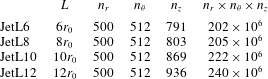
Four large-eddy simulations of a supersonic impinging jet impinging on a flat plate normally have been performed. The jet originates from a straight pipe nozzle of radius
 $r_{0}$
and diameter
 $D$
, and width
 $l=1.25r_{0}$
, whose lip is
 $0.1r_{0}$
thick, in an ambient medium at temperature
 $T_{0}=293$
K and pressure
 $p_{0}=10^{5}$
Pa. Nozzle-to-plate distances
 $L$
of
 $6r_{0}$
,
 $8r_{0}$
,
 $10r_{0}$
and
 $12r_{0}$
are considered. The four cases are consequently referred to as JetL6, JetL8, JetL10 and JetL12, as reported in table 1. At the nozzle exit, the jet is ideally expanded, and has a Mach number of
 ${\mathcal{M}}_{j}=u_{j}/a_{j}=1.5$
, and a Reynolds number of
 $Re_{j}=u_{j}D/\unicode[STIX]{x1D708}_{j}=6\times 10^{4}$
, where
 $u_{j}$
and
 $a_{j}$
are the jet velocity and the speed of sound and
 $\unicode[STIX]{x1D708}_{j}$
is the kinematic molecular viscosity and the stagnation temperature is equal to the ambient temperature. At the nozzle inlet, a Blasius laminar boundary-layer profile of thickness
 $0.15r_{0}$
and a Crocco–Busemann profile are imposed for velocity and density. The ejection conditions of the jet and the ratios between the nozzle-to-plate distances and the exit diameter in the simulations are identical to those in the experiments of Krothapalli et al. (Reference Krothapalli, Rajkuperan, Alvi and Lourenco1999). The four nozzle-to-plate distances in the LES are chosen because of the acoustic measurements available and because of their regular spacings.
Nozzle-to-plate distance
 $L$
and number of grid points
 $n_{r}$
,
 $n_{\unicode[STIX]{x1D703}}$
and
 $n_{z}$
.

In order to generate velocity fluctuations at the nozzle exit, low-amplitude random vortical disturbances, not correlated in the azimuthal direction, are added in the boundary layer in the nozzle, at
 $z=-r_{0}/2$
, using a procedure detailed in Bogey, Marsden & Bailly (Reference Bogey, Marsden and Bailly2011b
). The forcing strength is set to
 $\unicode[STIX]{x1D6FC}=0.03$
in all cases. The profiles of mean and root-mean-square (r.m.s.) axial velocities obtained at the nozzle exit are presented in figure 1. In figure 1(a), the mean velocity profiles are very similar, and correspond to a Blasius laminar boundary-layer profile of momentum thicknesses
 $\unicode[STIX]{x1D6FF}_{\unicode[STIX]{x1D703}}=0.016r_{0}$
. As for the radial distributions of the turbulence intensities in figure 1(b), they differ, and reach peak values
 $u_{e}^{\prime }/u_{j}$
of 5.2 %, 3.5 %, 2.8 % and 2.6 % for JetL6, JetL8, JetL10 and JetL12, respectively. Therefore, the velocity fluctuations at the nozzle exit are stronger as the nozzle-to-plate distance decreases.
Radial profiles at the nozzle exit (a) of mean axial velocity
 $\langle u_{z}\rangle$
and (b) of root-mean-square values of axial velocity fluctuations
 $u_{z}^{\prime }$
:
—— JetL6, — ⋅ — JetL8, – – – JetL10, and


2.2 Numerical parameters
The numerical methods and parameters are identical or very similar to those in recent simulations of supersonic impinging jets (Gojon et al. Reference Gojon, Bogey and Marsden2016; Gojon & Bogey Reference Gojon and Bogey2017).
The unsteady compressible Navier–Stokes equations are solved in a cylindrical coordinate system
 $(r,\unicode[STIX]{x1D703},z)$
by using an explicit six-stage Runge–Kutta algorithm for time integration, and low-dispersion explicit eleven-point finite differences for spatial derivation (Bogey & Bailly Reference Bogey and Bailly2004; Berland et al.
Reference Berland, Bogey, Marsden and Bailly2007). At the end of each time step, a sixth-order eleven-point filtering (Bogey, de Cacqueray & Bailly Reference Bogey, de Cacqueray and Bailly2009) is applied to the flow variables in order to remove grid-to-grid oscillations and to relax turbulent energy from scales at wavenumbers close to the grid cutoff wavenumber. Thus, the filtering acts as a subgrid-scale model in the LES (Bogey & Bailly Reference Bogey and Bailly2006, Reference Bogey and Bailly2009; Fauconnier, Bogey & Dick Reference Fauconnier, Bogey and Dick2013; Kremer & Bogey Reference Kremer and Bogey2015). The radiation conditions of Tam & Dong (Reference Tam and Dong1994) are implemented at the inflow and lateral boundaries of the computational domain. A sponge zone combining grid stretching and Laplacian filtering is also employed in order to damp the turbulent fluctuations before they reach the lateral boundaries. The axis singularity is treated with the method of Mohseni & Colonius (Reference Mohseni and Colonius2000). Notably, the first point close to the axis is located at
 $r=\unicode[STIX]{x0394}r/2$
, where
 $\unicode[STIX]{x0394}r$
is the radial mesh size near the axis. A reduction of the effective resolution near the origin of the polar coordinates is also implemented (Bogey, de Cacqueray & Bailly Reference Bogey, de Cacqueray and Bailly2011a
) in order to increase the time step of the simulation. The present numerical set-up has been used in past studies to simulate subsonic round jets (Bogey et al.
Reference Bogey, Marsden and Bailly2011b
; Bogey, Marsden & Bailly Reference Bogey, Marsden and Bailly2012a
,Reference Bogey, Marsden and Bailly
b
; Bogey & Marsden Reference Bogey and Marsden2016). In the present LES, adiabatic conditions are imposed at the nozzle walls and at the flat plate. A shock-capturing filtering is applied in order to avoid Gibbs oscillations near shocks. It consists in applying a conservative second-order filter at a magnitude determined each time step using a shock sensor (Bogey et al.
Reference Bogey, de Cacqueray and Bailly2009). It was successfully used by de Cacqueray, Bogey & Bailly (Reference de Cacqueray, Bogey and Bailly2011) for the LES of an overexpanded jet at an equivalent Mach number of
 ${\mathcal{M}}_{j}=3.3$
.
The simulations have been carried out using an OpenMP-based in-house solver, and a total of 100 000 iterations are computed in each case after the transient period. The temporal discretization is equal to
 $\unicode[STIX]{x0394}t=0.005r_{0}/u_{j}$
, yielding a simulation time of
 $500r_{0}/u_{j}$
. The meshes are directly derived from those used in recent LES of underexpanded impinging round jets (Gojon & Bogey Reference Gojon and Bogey2017). They contain between 202 and 240 million points, as noted in table 1 also yielding the number of points
 $n_{r}$
,
 $n_{\unicode[STIX]{x1D703}}$
and
 $n_{z}$
in the radial, azimuthal and axial directions. The variations of the radial and axial mesh spacings are represented in figure 2. The minimal axial mesh spacing is equal to
 $\unicode[STIX]{x0394}z=0.0075r_{0}$
near the nozzle lip and the flat plate, and the maximal axial mesh spacing between the nozzle and the plate is
 $\unicode[STIX]{x0394}z=0.015r_{0}$
for JetL6 and
 $\unicode[STIX]{x0394}z=0.03r_{0}$
in the three other cases. The minimal radial spacing is equal to
 $\unicode[STIX]{x0394}r=0.0075r_{0}$
at
 $r=r_{0}$
, and the maximal radial spacing is
 $\unicode[STIX]{x0394}r=0.06r_{0}$
for
 $5r_{0}\leqslant r\leqslant 15r_{0}$
. Farther from the jet axis, a sponge zone is implemented for
 $r\geqslant 15r_{0}$
. In the physical domain, the grids are stretched at rates lower than 1 % in order to preserve numerical accuracy. Note, moreover, that the maximum mesh spacing of
 $0.06r_{0}$
allows acoustic waves with Strouhal numbers up to
 $St=fD/u_{j}=6.1$
to be well propagated, where
 $f$
is the frequency.
Representation of (a) the radial and (b) the axial mesh spacings
 $\unicode[STIX]{x0394}r$
and
 $\unicode[STIX]{x0394}z$
:
—— JetL6, — ⋅ — JetL8, – – – JetL10, and


2.3 Flow snapshots
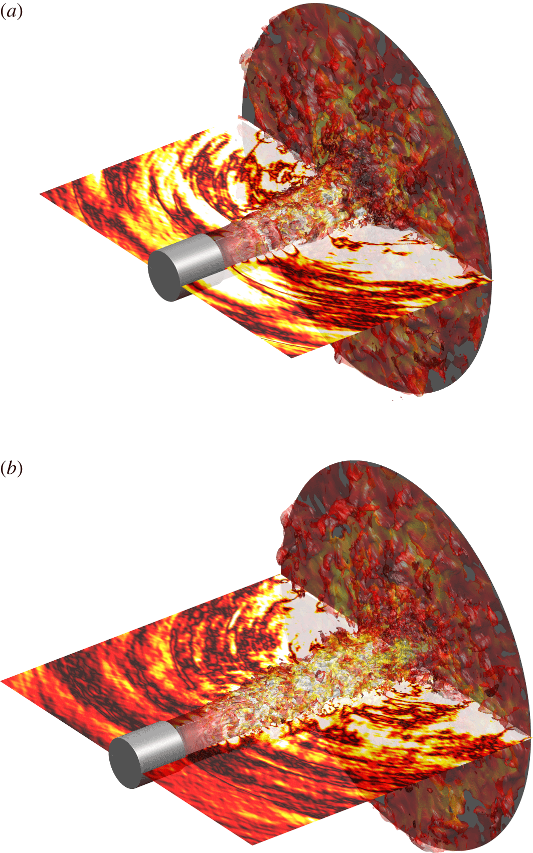
The jet flow and acoustic fields obtained for JetL8 and JetL12 are represented in figure 3 displaying 3-D isosurfaces of density and 2-D pressure fields in the planes
 $\unicode[STIX]{x1D703}=0$
and
 $\unicode[STIX]{x1D703}=\unicode[STIX]{x03C0}$
. The jet shear layers appear weakly disturbed in the vicinity of the nozzle exit, but exhibit both small- and large-scale turbulent structures for
 $z>2r_{0}$
, as expected at a Reynolds number of
 $6\times 10^{4}$
. Farther downstream, the development of wall jets on the flat plate after the jet impact is clearly visible. As for the near pressure fields, they show acoustic waves mainly propagating in the upstream direction, which seem to be generated in the region of jet impingement.
Representation for (a) JetL8 and (b) JetL12 of the isosurfaces of density associated with
 $1.3~\text{kg}~\text{m}^{-3}$
, coloured by the local Mach number, and of the pressure
 $p-p_{0}$
at
 $\unicode[STIX]{x1D703}=0$
and
 $\unicode[STIX]{x03C0}$
using a colour scale ranging from
 $-3000$
to 3000 Pa, from white to red; nozzle and flat plate in grey.

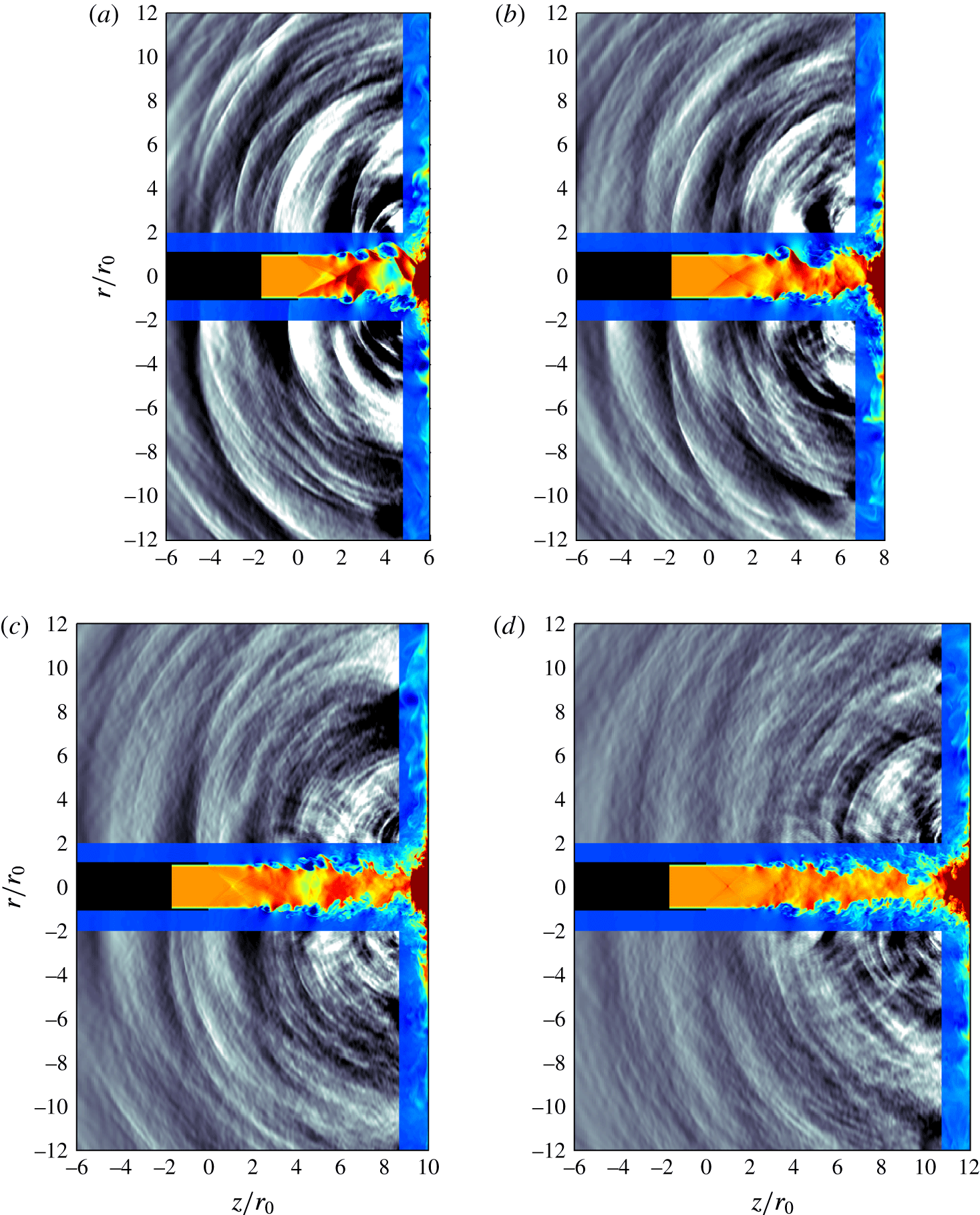
Density and fluctuating pressure fields obtained in the
 $(z,r)$
plane for the four impinging jets are provided in figure 4 and in movie 1 available at https://doi.org/10.1017/jfm.2017.334. In all cases, large-scale turbulent structures and sound waves are observed in the shear layers and outside the jet, respectively. Strong acoustic waves appear to propagate in the upstream direction from the region of jet impact. Their amplitudes decrease as the nozzle-to-plate distance increases. For jetL8, jetL10 and jetL12, circular waves centred around
 $z\simeq 3r_{0}$
in the jet shear layers are also visible. Looking at the movie, they seem to result from the interactions of the upstream-propagating acoustic waves with the shear-layer turbulent structures.
Snapshots in the
 $(z,r)$
plane of density in the jet and near the flat plate and of pressure
 $p-p_{0}$
for (a) JetL6, (b) JetL8, (c) JetL10 and (d) JetL12. The colour scales range from 1 to
 $2~\text{kg}~\text{m}^{-3}$
for density, from blue to red, and from
 $-5000$
to 5000 Pa for pressure, from black to white. The nozzle is in black.

2.4 Flow field properties
The variations of the mean axial velocity on the jet centreline and of the shear-layer momentum thickness between the nozzle exit at
 $z=0$
and the flat plate at
 $z=L$
are presented in figure 5. In figure 5(a), in all cases, the centreline mean velocity remains very close to the exit velocity
 $u_{j}$
down to approximately
 $z=L-r_{0}$
, with a maximum deviation of only 3.5 % of
 $u_{j}$
, which supports that the jets are nearly ideally expanded. For
 $z\geqslant L-r_{0}$
, the centreline velocity decreases sharply to become nil at the wall. Note that for a free jet at the same Mach number as the present impinging jets, the potential core is expected to close farther from
 $z=12r_{0}$
, and more precisely at
 $z=13.3r_{0}$
according to Lau, Morris & Fisher (Reference Lau, Morris and Fisher1979).
As for the shear-layer momentum thickness in figure 5(b), it does not vary much up to
 $z=0.95$
, where the end of a very weak shock cell is most likely located in the jets as suggested by figure 5(a). Farther downstream, it increases nearly linearly before reaching a peak just upstream of the flat plate at
 $z\simeq L-r_{0}$
. The profile obtained for JetL6 is systematically above those for JetL8, JetL10 and JetL12 which are almost superimposed for
 $z\leqslant 5r_{0}$
. The spreading of the shear layers is therefore accelerated by the presence of the plate in the former case, but poorly affected in the three others.
Variations (a) of the mean axial velocity
 $\langle u_{z}\rangle$
on the jet centreline, and (b) of the shear-layer momentum thickness
 $\unicode[STIX]{x1D6FF}_{\unicode[STIX]{x1D703}}$
:
—— JetL6, — ⋅ — JetL8, – – – JetL10, and


The r.m.s. values of axial velocity fluctuations estimated at
 $r=0$
and
 $r=r_{0}$
are shown in figure 6. Overall, the profiles display similar shapes for the four jets, but higher levels of velocity fluctuations for shorter nozzle-to-plate distances. On the jet axis, in figure 6(a), the turbulent intensities are negligible up to
 $z\simeq r_{0}$
, then gently increase with the axial distance and reach strong peak values at
 $z\simeq L-0.8r_{0}$
, ranging from 21.5 % for JetL6 down to 13.4 % for JetL12. On the nozzle lip line, in figure 6(b), the growth of the turbulent intensities starts at the nozzle exit and happens rapidly. Farther downstream, two humps are found: one around
 $z=3.3r_{0}$
, and another just upstream of the flat plate. The maximum levels obtained vary from 22 % down to 18.6 % at the first location and from 22.8 % down to 20.5 % at the other.
Variations of the root-mean-square values of axial velocity fluctuations
 $u_{z}^{\prime }$
(a) at
 $r=0$
and (b) at
 $r=r_{0}$
:
—— JetL6, — ⋅ — JetL8, – – – JetL10, and


2.5 Convection velocity
In most models of the feedback loop establishing in impinging jets, the convection velocity of the turbulent structures in the shear layers is required to describe the aerodynamic part of the loop. The variations of the local convection velocity
 $u_{c}$
estimated in the present jets at
 $r=r_{0}$
from cross-correlations of axial velocity fluctuations are thus represented in figure 7(a). As observed in previous simulations (Gojon et al.
Reference Gojon, Bogey and Marsden2016; Gojon & Bogey Reference Gojon and Bogey2017), the convection velocity grows with the axial distance, from approximately
 $0.5u_{j}$
near the nozzle exit up to
 $0.65u_{j}$
much farther downstream.
The average convection velocities
 $\langle u_{c}\rangle$
then calculated between the jet nozzle and the flat plate are displayed in figure 7(b) as a function of the nozzle-to-plate distance. They increase with
 $L/r_{0}$
, as in the experiments of Krothapalli et al. (Reference Krothapalli, Rajkuperan, Alvi and Lourenco1999). Ranging from
 $0.58u_{j}$
for JetL6 up to
 $0.62u_{j}$
for JetL12, they appear to be well predicted by the equation
 $$\begin{eqnarray}\langle u_{c}\rangle (L/r_{0})=0.65u_{j}-(0.65u_{j}-0.5u_{j})\times {\displaystyle \frac{1}{1+0.15(L/r_{0})^{2}}},\end{eqnarray}$$
which tends to
 $0.65u_{j}$
for large
 $L/r_{0}$
and to
 $0.5u_{j}$
for small
 $L/r_{0}$
.
Representation (a) of the convection velocity
 $u_{c}$
at
 $r=r_{0}$
for —— JetL6, — ⋅ — JetL8, – – – JetL10, and

 $\langle u_{c}\rangle$
between the nozzle and the plate from
 $\times$
LES and


2.6 Velocity spectra
The spectra of axial velocity fluctuations calculated on the lip line at the three axial locations
 $z=0.25r_{0}$
,
 $z=r_{0}$
and
 $z=4r_{0}$
are presented in figure 8 as a function of the Strouhal number
 $St=fD/u_{j}$
. At the first location very near the nozzle, several tones emerge at Strouhal numbers below 1, with dominant tones at
 $St=0.455$
in JetL6, 0.445 in JetL8, 0.44 in JetL10 and 0.38 in JetL12. The same tones will be found in the near-nozzle pressure spectra in the next section. They correspond to the tones generated by the aeroacoustic feedback loop establishing between the nozzle and the flat plate. At the second location, at
 $z=r_{0}$
, the highest levels are still obtained at the tone frequencies, but another instability-like component is observed for
 $St>0.8$
in all cases. This extra component is non-tonal, and centred around
 $St\simeq 1.8$
, yielding Strouhal numbers based on the nozzle exit momentum thickness of
 $St_{\unicode[STIX]{x1D703}}=f\unicode[STIX]{x1D6FF}_{\unicode[STIX]{x1D703}}/u_{j}\simeq 0.014$
. This peak frequency falls within the range of frequencies predominating early on in unforced initially laminar mixing layers according to linear stability analyses (Michalke Reference Michalke1984) and experiments (Gutmark & Ho Reference Gutmark and Ho1983). Further downstream, at
 $z=4r_{0}$
, the velocity spectra display broadband shapes. The contribution of the tones are however visible, especially for small flat-to-plate distances.
Power spectral densities (PSD) of axial velocity fluctuations
 $u_{z}^{\prime }$
obtained at
 $r=r_{0}$
, at ——
 $z=0.25r_{0}$
,

 $z=r_{0}$
and

 $z=4r_{0}$
, as a function of
 $St$
, in
 $\text{dB}/St$
: (a) JetL6, (b) JetL8, (c) JetL10 and (d) JetL12.

2.7 Pressure spectra and tone frequencies
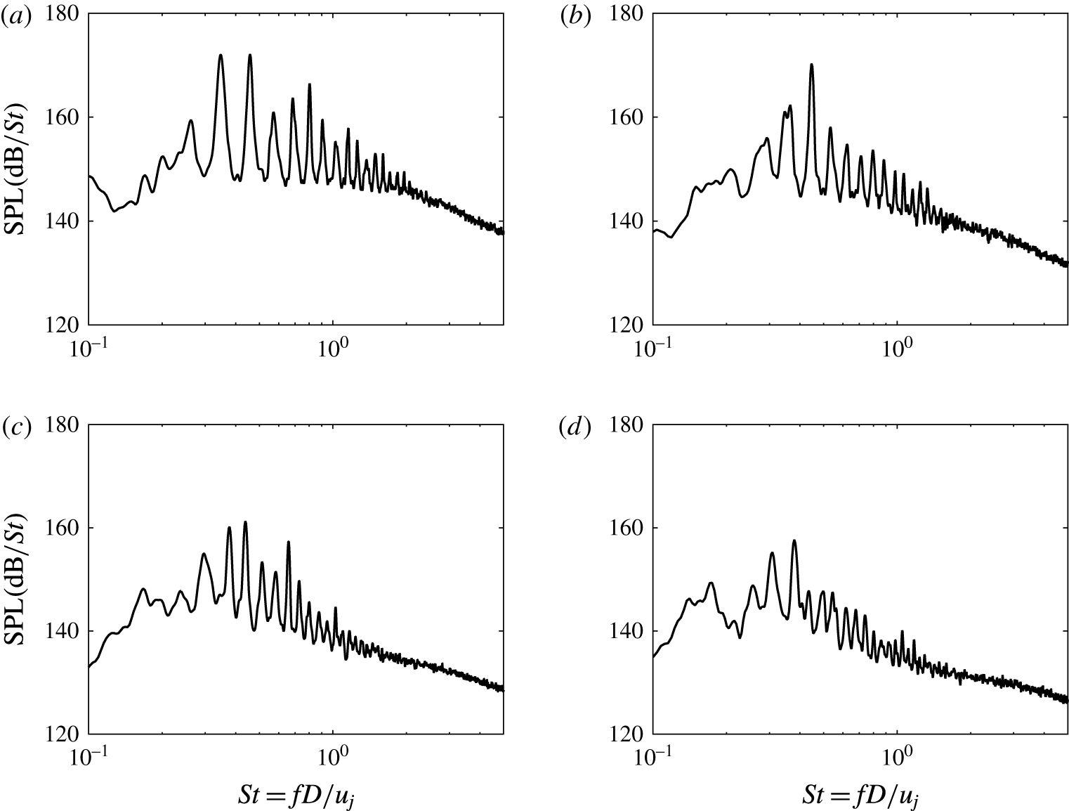
The pressure spectra obtained at
 $z=0$
and
 $r=2r_{0}$
for the different jets are represented in figure 9 as a function of the Strouhal number. They are very similar to the velocity spectra computed at
 $z=0.25r_{0}$
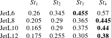
in the shear layer, shown in figure 8. A large number of tones emerge, as observed experimentally by Norum (Reference Norum1991) and Krothapalli et al. (Reference Krothapalli, Rajkuperan, Alvi and Lourenco1999), among others, for rectangular and round ideally expanded impinging jets. In the present cases, the dominant tones with the highest amplitude are found at
 $St=0.455$
in JetL6, 0.445 in JetL8, 0.44 in JetL10 and 0.38 in JetL12, thus remaining in the same range of frequencies. Their levels are more than 10 dB higher than the broadband noise level, and decrease with the nozzle-to-plate distance, which is consistent with recent LES results for ideally expanded planar jets (Gojon et al.
Reference Gojon, Bogey and Marsden2016) and with the reduction in turbulent intensities with
 $L/r_{0}$
reported in § 2.5.
The Strouhal numbers
 $St_{1}$
,
 $St_{2}$
,
 $St_{3}$
and
 $St_{4}$
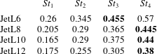
of the first four tones in the pressure spectra are collected in table 2. These tones include the dominant tones, which are the third or the fourth tones in all cases, and a first low-frequency tone at
 $St_{1}$
varying between 0.165 in JetL10 up to 0.26 in JetL6. This tone is weak, especially in JetL8 and JetL10, but it is provided here because it will be considered in the analysis of the feedback loop conducted in § 3. On the contrary, the tones at Strouhal numbers
 $St>St_{4}$
are disregarded because most of them are harmonics of the first four tones. This is the case for instance for JetL6, for which these tones are found at
 $St_{5}=0.69=2St_{2}$
,
 $St_{6}=0.80=St_{2}+St_{3}$
and
 $St_{7}=0.90=2St_{3}$
. Note that the first four tone frequencies will be compared with the experimental data of Krothapalli et al. (Reference Krothapalli, Rajkuperan, Alvi and Lourenco1999) in § 3.1.
Sound pressure levels (SPL) obtained at
 $z=0$
and
 $r=2r_{0}$
as a function of Strouhal number
 $St$
: (a) JetL6, (b) JetL8, (c) JetL10 and (d) JetL12.

Strouhal numbers of the first four tones emerging in the spectra of figure 9; dominant tones in bold.
2.8 Fourier decomposition of the pressure field
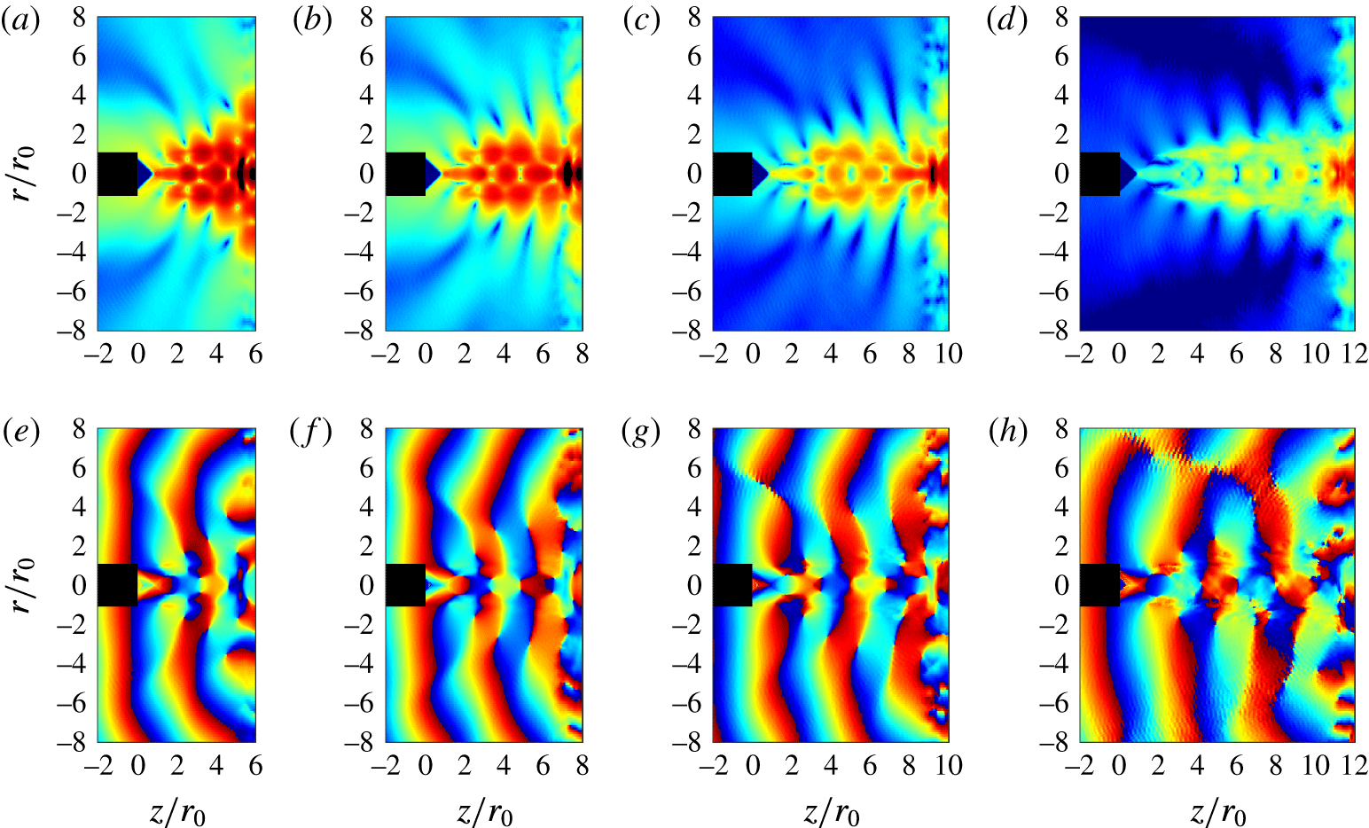
In order to determine the amplitude and phase fields associated with the different tones of the jets, a Fourier transform in time has been applied to the near pressure fields recorded every 50th LES time step in the
 $(z,r)$
plane. The results obtained at the dominant tone frequencies are represented in figure 10. The amplitude fields in the top views exhibit cell structures between the jet nozzle and the flat plate. By considering the two semi-cells near the nozzle and the plate as one cell, the structures contain a whole number of cells
 $N_{sw}$
, namely 4 cells in JetL6, 5 cells in JetL8, and 6 cells in JetL10 and JetL12. They are due to the presence of hydrodynamic-acoustic standing waves at the tone frequencies, with wavenumbers equal to
 $$\begin{eqnarray}k_{sw}=k_{p}+k_{a}=\frac{2\unicode[STIX]{x03C0}N_{sw}}{L},\end{eqnarray}$$
where
 $k_{p}$
and
 $k_{a}$
are the wavenumbers of the hydrodynamic and acoustic waves (Panda, Raman & Zaman Reference Panda, Raman and Zaman1997; Gojon et al.
Reference Gojon, Bogey and Marsden2016).
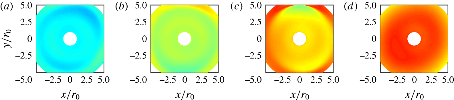
As for the three-dimensional organization of the jet pressure fields at the dominant tone frequencies, it is revealed by the phase fields in the bottom views of figure 10, and by those obtained for the pressure at
 $z=0$
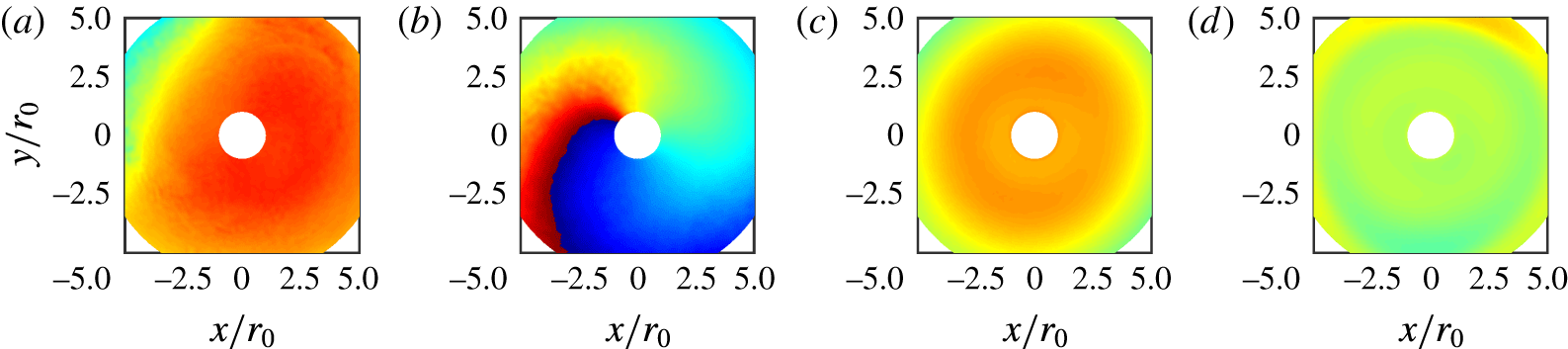
, provided in figure 11. In all cases, the phase is identical on both sides of the jet in the first figure, and does not vary appreciably in the azimuthal direction on the second figure. These results indicate that the jet oscillations are axisymmetric at the frequencies considered.
Amplitude (a–d) and phase (e–h) fields obtained for the pressure at the dominant tone frequencies in (a,e) JetL6 at
 $St=0.455$
, (b,f) JetL8 at
 $St=0.445$
, (c,g) JetL10 at
 $St=0.44$
and (d,h) JetL12 at
 $St=0.38$
. The colour scales range from 115
 $\text{dB}/St$
to 165
 $\text{dB}/St$
and from
 $-\unicode[STIX]{x03C0}$
to
 $\unicode[STIX]{x03C0}$
, respectively, from blue to red.

Phase fields obtained for the pressure at the dominant tone frequencies in (a) JetL6, (b) JetL8, (c) JetL10 and (d) JetL12; colour scale from
 $-\unicode[STIX]{x03C0}$
to
 $\unicode[STIX]{x03C0}$
, from blue to red.

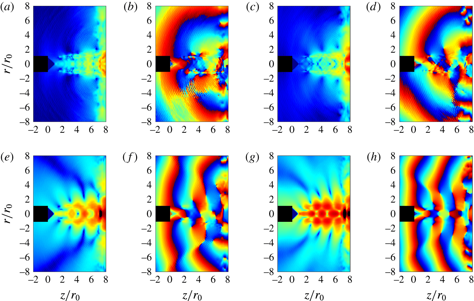
The amplitude and phase fields obtained for JetL8 at the four tone frequencies given in table 2 are displayed in figure 12. In the top views, the standing-wave patterns contain 2 cells at Strouhal number
 $St_{1}$
, 3 cells at
 $St_{2}$
, 4 cells at
 $St_{3}$
and 5 cells at
 $St_{4}$
. In the bottom views, the phase fields appear symmetric with respect to the jet axis at
 $St_{1}$
,
 $St_{3}$
and
 $St_{4}$
, and antisymmetric at
 $St_{2}$
. Moreover, the phase fields computed from for the pressure at
 $z=0$
are shown in figure 13. In the azimuthal direction, the phase remains nearly constant at
 $St_{1}$
,
 $St_{3}$
and
 $St_{4}$
, but varies by
 $2\unicode[STIX]{x03C0}$
at
 $St_{2}$
. Therefore, the modes of jet oscillation are the axisymmetric mode at the frequencies of the first, third and fourth tones, and the first helical mode at the frequency of the second tone.
The results obtained for the other jets are reported in table 3.
Amplitude and phase fields obtained for the pressure in JetL8 at the tone Strouhal numbers of (a,b)
 $St_{1}=0.205$
, (c,d)
 $St_{2}=0.29$
, (e,f)
 $St_{3}=0.365$
and (g,h)
 $St_{4}=0.445$
. The colour scales range from 115
 $\text{dB}/St$
to 165
 $\text{dB}/St$
, and from
 $-\unicode[STIX]{x03C0}$
to
 $\unicode[STIX]{x03C0}$
, respectively, from blue to red.

Phase fields obtained for the pressure in JetL8 at (a)
 $St_{1}$
, (b)
 $St_{2}$
, (c)
 $St_{3}$
and (d)
 $St_{4}$
; colour scale from
 $-\unicode[STIX]{x03C0}$
to
 $\unicode[STIX]{x03C0}$
, from blue to red.

Number of cells in the standing waves and axisymmetric or helical nature of the jet oscillations at the first four tone Strouhal numbers.

3 Modelling of the feedback loop
3.1 Aeroacoustic feedback model
As pointed out in the introduction, it has been well known since the work of Powell (Reference Powell1953) that the tones generated by impinging jets are due a feedback mechanism between the nozzle lips and the flat plate, involving aerodynamic disturbances growing and convected downstream in the jets and acoustic waves travelling in the upstream direction. In the feedback model of Ho & Nosseir (Reference Ho and Nosseir1981) and Nosseir & Ho (Reference Nosseir and Ho1982), these acoustic waves are assumed to propagate outside the jets. By considering that the fundamental period of the feedback loop is given by the sum of the time necessary for shear-layer disturbances to travel from the nozzle down to the plate and of the time of propagation of acoustic waves from the plate up to the nozzle, the relation
 $$\begin{eqnarray}{\displaystyle \frac{L}{\langle u_{c}\rangle }}+{\displaystyle \frac{L}{a_{0}}}={\displaystyle \frac{N}{f}}\end{eqnarray}$$
was obtained, where
 $\langle u_{c}\rangle$
is the average convection velocity in the shear layers,
 $a_{0}$
is the speed of sound outside of the jet and
 $N$
is the mode number.
The Strouhal numbers of the four tones given in table 2 for the present jets are represented in figure 14 as a function of the nozzle-to-plate distance. In figure 14(a), the tone frequencies measured in the experiments of Krothapalli et al. (Reference Krothapalli, Rajkuperan, Alvi and Lourenco1999) and those estimated from relation (3.1) using the average convection velocity provided by (2.1) are also plotted. The tone Strouhal numbers in the LES are comparable with the experimental data or, when this is not true, are located on the paths followed by these data as
 $L/r_{0}$
varies. For JetL6, for example, the first case is observed for the first and fourth tones, the second case for the second and third tones. Furthermore, the tone frequencies seem to be approximately predicted by the feedback model. In this way, the tones can be associated with different feedback modes: modes 2, 3, 4 and 5 for JetL6 and JetL8, modes 2, 4, 5 and 6 for JetL10 and modes 3, 4, 5 and 6 for JetL12. As expected (Gojon et al.
Reference Gojon, Bogey and Marsden2016), the mode numbers
 $N$
correspond to the number of cells
 $N_{sw}$
in the standing-wave patterns. Regarding the main tones, they can be related to the fourth feedback mode in JetL6, to the fifth mode in JetL8 and to the sixth mode in JetL10 and JetL12. A similar switch of the dominant tone frequency as the nozzle-to-plate distance increases was noted in the experiments of Krothapalli (Reference Krothapalli1985) for a rectangular supersonic impinging jet. Such a staging behaviour is also encountered in other self-oscillating flows, such as the flow over a cavity for instance (Rockwell & Naudascher Reference Rockwell and Naudascher1978).
Representation of the tone Strouhal numbers as a function of the nozzle-to-plate distance: (a) ▫ dominant and ● secondary tone frequencies in the LES,
 $\times$
experimental data of Krothapalli et al. (Reference Krothapalli, Rajkuperan, Alvi and Lourenco1999) and


 $St=0.225$
, 0.355 and 0.5.

In figure 14(b), the LES tone frequencies are represented alone using different symbols according to the axisymmetric or helical nature of the associated oscillation modes. By also plotting arbitrary horizontal lines on the figure, they clearly appear to be arranged in bands corresponding respectively, as the Strouhal number increases, to the axisymmetric mode for
 $St<0.225$
, the helical mode for
 $0.225<St<0.355$
, the axisymmetric mode for
 $0.355<St<0.5$
and the helical mode for
 $St>0.5$
. This behaviour cannot be explained by the feedback model reported above. For that reason, an alternative feedback model, in which the acoustic feedback waves do not only travel outside of the jet, is considered in what follows.
3.2 Analysis of the upstream-propagating acoustic wave modes of the jet
In the modified feedback model proposed by Tam & Ahuja (Reference Tam and Ahuja1990), and later extended by Tam & Norum (Reference Tam and Norum1992), it is assumed that the feedback loop in high-speed impinging jets is closed by waves belonging to the upstream-propagating acoustic wave modes of the jets. These waves were clearly identified in the theoretical study of Tam & Hu (Reference Tam and Hu1989), and their importance to the capture of a feedback link from acoustic disturbances downstream was recently emphasized by Nichols & Lele (Reference Nichols and Lele2011). They were recently detected in the potential core of subsonic free jets by Towne et al. (Reference Towne, Cavalieri, Jordan, Colonius, Jaunet, Schmidt and Brès2016). As with the familiar Kelvin–Helmholtz instability waves, they are instability waves that can be determined from the jet mean flow (Berman & Williams Reference Berman and Williams1970; Mack Reference Mack1990; Sabatini & Bailly Reference Sabatini and Bailly2014).
In this work, they are characterized for an ideally expanded round jet of radius
 $r_{0}$
and velocity
 $u_{j}$
with the same Mach number
 ${\mathcal{M}}_{j}=1.5$
as the present jets. The jet is modelled as a uniform stream bounded by a vortex street. The mathematical developments necessary to derive the dispersion relations of the upstream-propagating acoustic waves in a round jet using a vortex-sheet jet model that can be found in Tam & Ahuja (Reference Tam and Ahuja1990). By starting from the linearized governing equations for a compressible inviscid fluid, and noting that the waves considered here are neutral for a vortex-sheet jet model, i.e. that they have both real wavenumber
 $k$
and angular frequency
 $\unicode[STIX]{x1D714}$
, these authors obtained the following relations
 $$\begin{eqnarray}\displaystyle & & \displaystyle |\unicode[STIX]{x1D709}_{+}|J_{n}(|\unicode[STIX]{x1D709}_{-}\unicode[STIX]{x1D6FC}|){\displaystyle \frac{K_{n-1}(|\unicode[STIX]{x1D709}_{+}\unicode[STIX]{x1D6FC}|)+K_{n+1}(|\unicode[STIX]{x1D709}_{+}\unicode[STIX]{x1D6FC}|)}{K_{n}(|\unicode[STIX]{x1D709}_{+}\unicode[STIX]{x1D6FC}|)}}\nonumber\\ \displaystyle & & \displaystyle \quad +\,{\displaystyle \frac{C^{2}|\unicode[STIX]{x1D709}_{-}|}{(a_{0}C/a_{j}-{\mathcal{M}}_{j})^{2}}}[J_{n-1}(|\unicode[STIX]{x1D709}_{-}\unicode[STIX]{x1D6FC}|)-J_{n+1}(|\unicode[STIX]{x1D709}_{-}\unicode[STIX]{x1D6FC}|)]=0,\end{eqnarray}$$
where
 $a_{0}$
and
 $a_{j}$
are the sound speeds in the ambient medium and in the jet,
 $C=\unicode[STIX]{x1D714}/(ka_{0})$
,
 $J_{n}$
is the
 $n$
th-order Bessel function of the first kind,
 $\unicode[STIX]{x1D709}_{+}=|C^{2}-1|^{1/2}$
,
 $\unicode[STIX]{x1D709}_{-}=|(a_{0}C/a_{j}-{\mathcal{M}}_{j})^{2}-1|^{1/2}$
,
 $\unicode[STIX]{x1D6FC}=kr_{0}$
and
 $K_{n}$
is the
 $n$
th-order modified Bessel function.
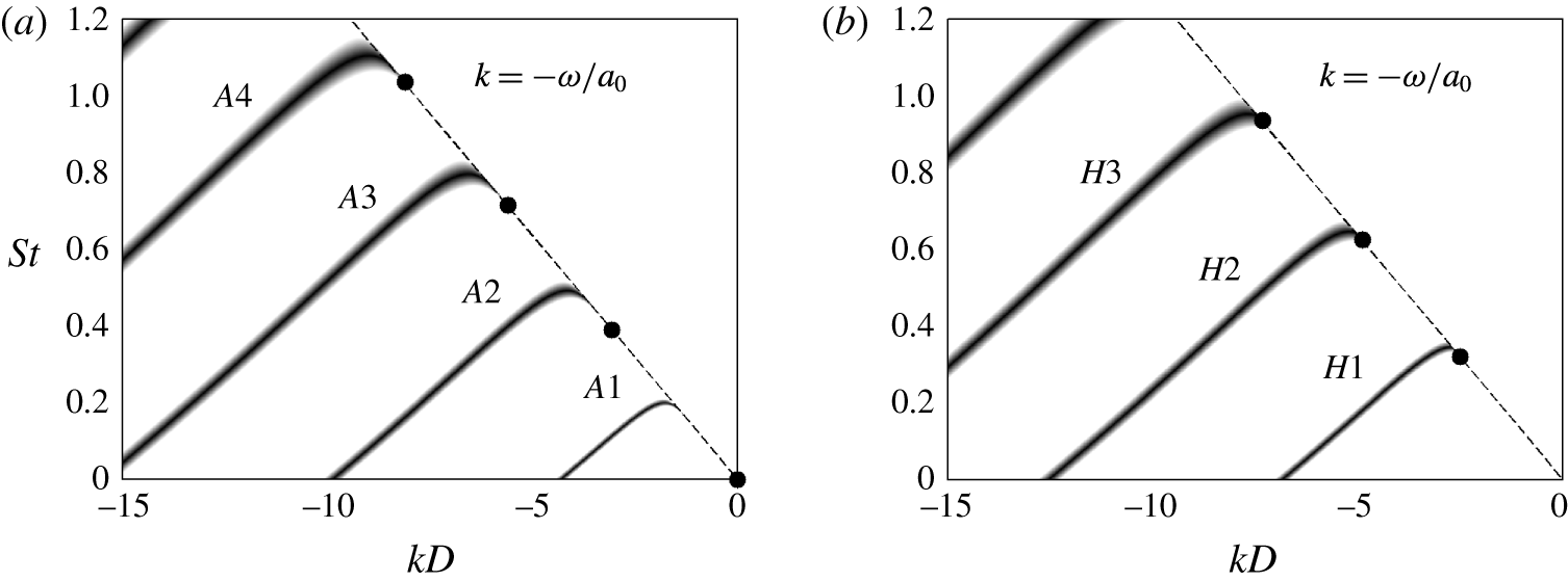
The solutions of the dispersion relations calculated for the present jet for the axisymmetric modes (
 $n=0$
) and the first helical modes (
 $n=1$
) are represented in figure 15 as functions of the Strouhal number and the wavenumber. For
 $St\leqslant 1.2$
, four axisymmetric neutral acoustic wave modes, referred to as
 $A1$
,
 $A2$
,
 $A3$
and
 $A4$
, and three helical modes denoted by
 $H1$
,
 $H2$
and
 $H3$
, appear.
Representation of the dispersion relations of the (a) axisymmetric and (b) helical neutral acoustic wave modes for an ideally expanded round jet at
 ${\mathcal{M}}_{j}=1.5$
; ● lower limits of the modes; – – –
 $k=-\unicode[STIX]{x1D714}/a_{0}$
.

For the different modes, the upstream-propagating acoustic waves are situated on the part of the dispersion curves where the slope
 $\text{d}St/\text{d}k$
and hence the group velocity
 $\text{d}\unicode[STIX]{x1D714}/\text{d}k$
are negative, which leads to the existence of allowable frequency ranges. Their upper and lower limits correspond to the maximum and minimum Strouhal numbers reached for the modes. The first ones are taken from the dispersion curves. The second ones can be calculated since they are necessarily associated with acoustic waves propagating with a group velocity of
 $-a_{0}$
, and located on the dashed line of figure 15 defined by
 $$\begin{eqnarray}k=-{\displaystyle \frac{\unicode[STIX]{x1D714}}{a_{0}}}.\end{eqnarray}$$
In this way, Tam & Ahuja (Reference Tam and Ahuja1990) demonstrated that the lower limit for the first axisymmetric mode
 $A1$
is at
 $St_{A0}^{min}=0$
, and that the lower limits for the axisymmetric modes
 $Ai$
with
 $i>0$
are
 $$\begin{eqnarray}St_{Ai}^{min}={\displaystyle \frac{\unicode[STIX]{x1D70E}_{i}}{\unicode[STIX]{x03C0}{\mathcal{M}}_{j}(a_{j}/a_{0})|(a_{0}/a_{j}+{\mathcal{M}}_{j})^{2}-1|^{1/2}}},\end{eqnarray}$$
where
 $\unicode[STIX]{x1D70E}_{i}$
is the
 $i$
th root of
 $J_{1}$
. For the first helical modes (
 $n=1$
), the lower limits
 $St_{Hi}^{min}$
are the roots of the equation
 $$\begin{eqnarray}2J_{1}(|\overline{\unicode[STIX]{x1D709}}_{-}\unicode[STIX]{x1D6FC}|)+{\displaystyle \frac{|\overline{\unicode[STIX]{x1D709}}_{-}\unicode[STIX]{x1D6FC}|}{((a_{0}/a_{j})+{\mathcal{M}}_{j})^{2}}}(J_{0}(|\overline{\unicode[STIX]{x1D709}}_{-}\unicode[STIX]{x1D6FC}|)-J_{2}(|\overline{\unicode[STIX]{x1D709}}_{-}\unicode[STIX]{x1D6FC}|))=0\end{eqnarray}$$
obtained from (3.2) as
 $k\rightarrow -\unicode[STIX]{x1D714}/a_{0}$
. The values computed for the modes
 $A1$
,
 $A2$
,
 $A3$
and
 $A4$
and
 $H1$
,
 $H2$
and
 $H3$
of the present jet using (3.5) and (3.5) are depicted in figure 15.
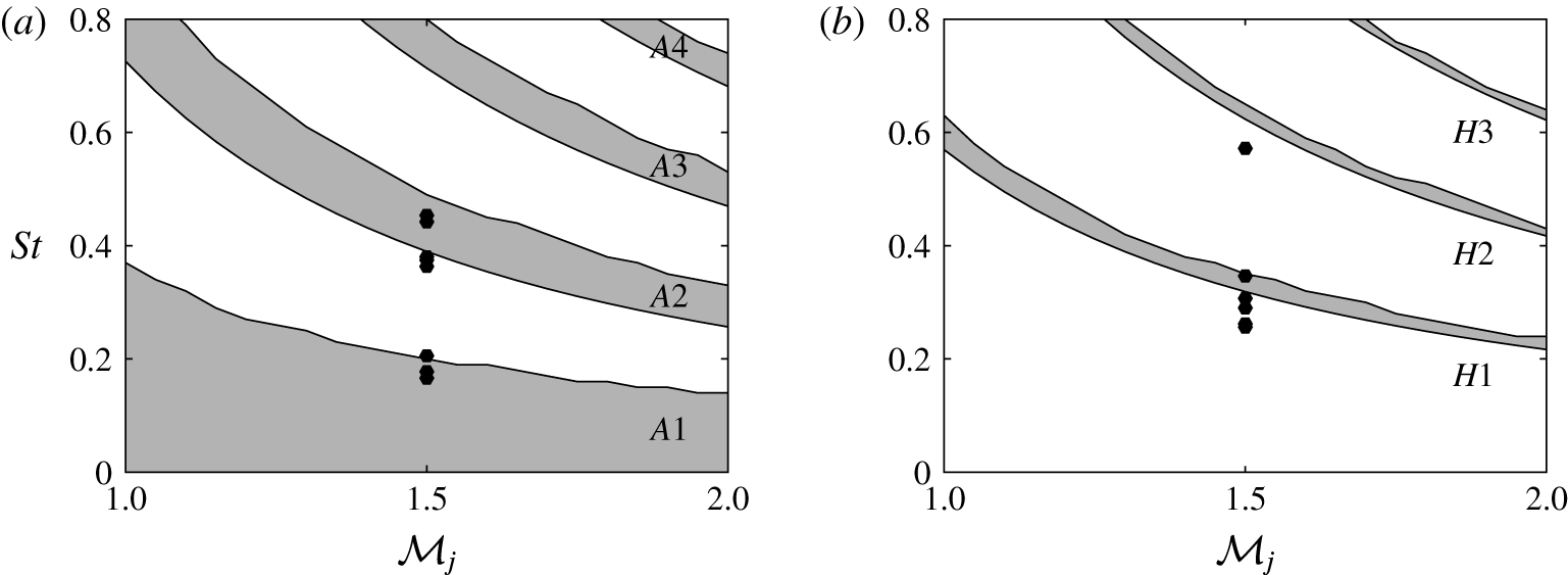
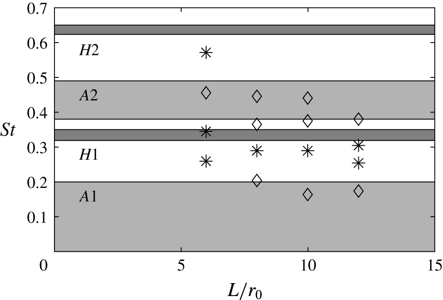
The allowable frequency ranges determined for the axisymmetric and the first helical upstream-propagating wave modes are represented in figure 16 as a function of the exit Mach number
 ${\mathcal{M}}_{j}$
. The first four tone frequencies of the simulated jets at
 ${\mathcal{M}}_{j}=1.5$
, given in table 2 in § 2.6, are also plotted. They are additionally displayed in figure 17 as a function of the nozzle-to-plate distance using different symbols according to the axisymmetric or helical nature of the associated oscillation modes, together with the allowable frequency ranges obtained for a Mach number of
 ${\mathcal{M}}_{j}=1.5$
.
The tones at Strouhal numbers
 $0.165\leqslant St\leqslant 0.205$
(first tones in JetL8, JetL10 and JetL12) fall in or just above the range of the mode
 $A1$
, and those at
 $0.365\leqslant St\leqslant 0.455$
(third tones in JetL6, JetL8 and JetL10 and fourth tones in JetL8, JetL10 and JetL12) lie in or just below the range of the mode
 $A2$
. The tones at
 $0.255\leqslant St\leqslant 0.345$
(first tone in JetL6, second tones in all cases and third tone in JetL12) and those at
 $St=0.57$
(fourth tone in JetL6) are located in most case below but close to the ranges of the modes
 $H1$
and
 $H2$
, respectively. These results are consistent with the axisymmetric or helical oscillations of the jet pressure fields at the tone frequencies, found in § 2.8 and reported in table 3. The disagreements observed, which are stronger for the helical modes than for the axisymmetric modes, may be due to the use of a vortex-sheet jet model instead of a jet with a mixing layer of finite thickness (Tam & Ahuja Reference Tam and Ahuja1990). Despite this, the analysis of the upstream-propagating acoustic wave modes seems to predict the nature of the oscillation modes of the present round impinging jets, as was previously the case for supersonic planar impinging jets (Tam & Norum Reference Tam and Norum1992; Gojon et al.
Reference Gojon, Bogey and Marsden2016). However, it does not provide information on which discrete frequencies will be selected, for a given nozzle-to-plate distance, over the ranges of the different modes.
Representation of the allowable frequency ranges for the (a) axisymmetric and (b) helical upstream-propagating neutral acoustic wave modes in an ideally expanded round jet as a function of the jet exit Mach number; ● tone frequencies in the LES.

Representation of the tone Strouhal numbers as a function of the nozzle-to-plate distance: LES tone frequencies associated with ♢ axisymmetric and * helical modes and allowable frequency ranges of the upstream-propagating neutral acoustic wave modes in an ideally expanded round jet at
 ${\mathcal{M}}_{j}=1.5$
.

3.3 Combination of the feedback model and the wave analysis
As carried out in Gojon et al. (Reference Gojon, Bogey and Marsden2016) for supersonic planar jets, the classical feedback model and the wave analysis presented above are combined. In order to achieve this, the acoustic wavenumber in the feedback loop is assumed to be equal to the opposite of the wavenumber
 $k$
of the upstream-propagating acoustic waves of the wave analysis. Thus, (2.2) relating the wavenumber
 $k_{sw}$
of the hydrodynamic-acoustic standing wave due to the feedback mechanism and the acoustic and hydrodynamic wavenumbers
 $k_{a}$
and
 $k_{p}$
yields
 $$\begin{eqnarray}f={\displaystyle \frac{N\langle u_{c}\rangle }{L}}+k{\displaystyle \frac{\langle u_{c}\rangle }{2\unicode[STIX]{x03C0}}}\end{eqnarray}$$
given that
 $N_{sw}=N$
,
 $k_{p}=2\unicode[STIX]{x03C0}f/\langle u_{c}\rangle$
and
 $k_{a}=-k$
. The solutions of this equation, which depend on the nozzle-to-plate distance, and those of the dispersion relations (3.2), which do not, can then be represented in the same figure.
This is done for JetL6 in figure 18 by showing the dispersion relations of the acoustic wave modes for a jet at
 ${\mathcal{M}}_{j}=1.5$
and the solutions of (3.6) for the first seven modes of the feedback mechanism as functions of the Strouhal number and the wavenumber. The first four tones of JetL6 are also indicated on the line
 $k=-\unicode[STIX]{x1D714}/a_{0}$
, using different symbols according to the axisymmetric or helical nature of the corresponding oscillation modes. In figure 18(a), the tone at
 $St_{3}=0.455$
is located at the intersection of the curve for the axisymmetric mode
 $A2$
of the jet and of the line for the mode
 $N=4$
of the feedback loop. In figure 18(b), the tones at
 $St_{1}=0.26$
,
 $St_{2}=0.345$
and
 $St_{4}=0.57$
are on or just below the curves for the helical mode
 $H1$
in the first two cases and for the mode
 $H2$
in the third one, and near the lines associated with the modes
 $N=2$
,
 $N=3$
and
 $N=5$
of the feedback loop, respectively.
Representation of —— the dispersion relations of the (a) axisymmetric and (b) helical neutral acoustic wave modes for an ideally expanded round jet at
 ${\mathcal{M}}_{j}=1.5$
, ● lower limits of the modes; – – –
 $k=-\unicode[STIX]{x1D714}/a_{0}$
;

 $L=6r_{0}$
; LES tone frequencies of JetL6 associated with ♢ axisymmetric and * helical modes.

In the same way, the results of the model combination for JetL8, JetL10 and JetL12, and the first four tones in these jets, are displayed in figures 19–21 as functions of the Strouhal number and the wavenumber. For JetL8, in figure 19, the tone at
 $St_{1}=0.205$
lies on the curve for the axisymmetric mode
 $A1$
and near the line for the feedback mode
 $N=2$
, the tone at
 $St_{2}=0.29$
is just below the curve of the helical mode
 $H1$
and near the feedback mode
 $N=3$
, and the tones at
 $St_{3}=0.365$
and
 $St_{4}=0.445$
are close to the intersection points of the axisymmetric mode
 $A2$
and the feedback modes
 $N=4$
and
 $N=5$
. For JetL10, in figure 20, the first four tones of the jet at
 $St_{1}=0.165$
,
 $St_{2}=0.29$
,
 $St_{3}=0.375$
and
 $St_{4}=0.44$
stand on the curve for the mode
 $A1$
for
 $St_{1}$
, and close to the lower limits of the modes
 $H1$
for
 $St_{2}$
and
 $A2$
for
 $St_{3}$
and
 $St_{4}$
, and near the lines associated with the feedback modes
 $N=2$
,
 $N=4$
,
 $N=5$
and
 $N=6$
. Finally, for JetL12, in figure 21, the tones of the jet are on the curve of the mode
 $A1$
for
 $St_{1}$
, in the vicinity of the lower limits of the modes
 $H1$
for
 $St_{2}$
and
 $St_{3}$
and
 $A2$
for
 $St_{4}$
, and very close to the lines for the feedback modes
 $N=3$
,
 $N=4$
,
 $N=5$
and
 $N=6$
.
Representation of —— the dispersion relations of the (a) axisymmetric and (b) helical neutral acoustic wave modes for an ideally expanded round jet at
 ${\mathcal{M}}_{j}=1.5$
, ● lower limits of the modes; – – –
 $k=-\unicode[STIX]{x1D714}/a_{0}$
;

 $L=8r_{0}$
; LES tone frequencies of JetL8 associated with ♢ axisymmetric and * helical modes.

Representation of —— the dispersion relations of the (a) axisymmetric and (b) helical neutral acoustic wave modes for an ideally expanded round jet at
 ${\mathcal{M}}_{j}=1.5$
, ● lower limits of the modes; – – –
 $k=-\unicode[STIX]{x1D714}/a_{0}$
;

 $L=10r_{0}$
; LES tone frequencies of JetL10 associated with ♢ axisymmetric and * helical modes.

Representation of —— the dispersion relations of the (a) axisymmetric and (b) helical neutral acoustic wave modes for an ideally expanded round jet at
 ${\mathcal{M}}_{j}=1.5$
, ● lower limits of the modes; – – –
 $k=-\unicode[STIX]{x1D714}/a_{0}$
;

 $L=12r_{0}$
; LES tone frequencies of JetL12 associated with ♢ axisymmetric and * helical modes.

The above results are in agreement with the properties of the jet pressure fields revealed in § 2.8, and summarized in table 3. Therefore, the model combination appears able to predict at the same time the tone frequencies and mode number of the feedback mechanism, and the antisymmetric or symmetric nature of the associated oscillation modes. For all modes except for the axisymmetric mode
 $A1$
whose minimum Strouhal number is zero, the tones are located just above or below the lower limits of the modes, the latter case being probably due to the use of a vortex-sheet model (Tam & Ahuja Reference Tam and Ahuja1990). Given that on the dispersion curves, the waves have a group velocity, but also a phase velocity very close to
 $-a_{0}$
near the lower limits of the modes, the model combination seems to indicate that the tones which are likely to be generated are those for which the feedback loop is closed by waves with such velocities. This is also one assumption made for the feedback waves of the classical aeroacoustic feedback model, which may explain the validity of (3.1). Furthermore, the model combination helps us to clarify why certain tones do not emerge. This is the case for instance in JetL10 for the tone associated with the mode
 $N=3$
of the feedback loop. Indeed, the line corresponding to that mode in figure 20(a) intersects on the dispersion curve for the mode
 $A1$
in a region where the group velocity, albeit negative, differs strongly from
 $-a_{0}$
, and this line in figure 20(b) is too far below the dispersion curve for the mode
 $H1$
.
An additional indirect evidence of the role of the neutral acoustic wave modes in the upstream part of feedback loop is provided by the amplitude fields obtained for the pressure at the frequencies of the tones associated with axisymmetric oscillations. For JetL8, for instance, the levels are very small along a line around
 $r=0.5r_{0}$
for
 $St_{3}=0.365$
and
 $St_{4}=0.445$
in figure 12(c–d), which is not true for
 $St_{1}=0.205$
in figure 12(a). This is consistent with the eigenfunction distributions of the neutral acoustic wave modes
 $A2$
and
 $A1$
, given by Tam & Ahuja (Reference Tam and Ahuja1990) for
 ${\mathcal{M}}_{j}=1.4$
, which reach a zero value at
 $r=0.5r_{0}$
in the former case, but not in the latter.
3.4 Upstream-propagating waves in the jets
An attempt is now made to directly detect the upstream-propagating waves mentioned above in the present jets, as recently done by Towne et al. (Reference Towne, Cavalieri, Jordan, Colonius, Jaunet, Schmidt and Brès2016) in the potential core of subsonic free jets. For that purpose, the LES pressure and density fields are re-examined, and pressure spectra are computed in the frequency–wavenumber space.
Snapshots of the pressure obtained for JetL12 in the
 $(z,r)$
plane over
 $0\leqslant z\leqslant 4r_{0}$
are provided in figure 22 at twelve consecutive times separated by
 $0.28r_{0}/u_{j}$
or
 $0.22r_{0}/a_{0}$
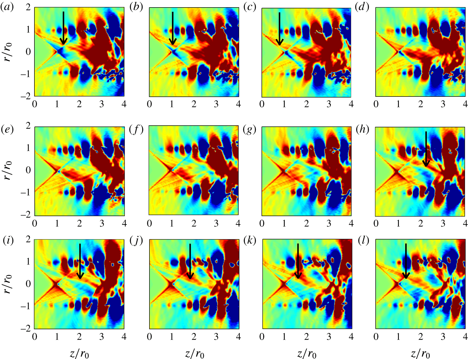
. A weak shock cell structure appears to form near the nozzle exit, as suggested previously by the centreline profile of mean velocity of figure 5. Kelvin–Helmholtz instability waves also develop and travel downstream in the jet shear layers. More importantly, waves are clearly found to propagate upstream inside the supersonic jet core. These waves are also well visible in the density fields of the four jets, which are given in movie 1 available as supplementary material. They look like oblique waves trapped inside the jet column. Some of these waves seem symmetric with respect to the jet axis as in figure 22(a–d), or antisymmetric as in figure 22(h–l).
Representation of the pressure
 $p-p_{0}$
obtained at
 $\unicode[STIX]{x1D703}=0$
and
 $\unicode[STIX]{x03C0}$
for JetL12 at twelve consecutive times separated by
 $0.28r_{0}/u_{j}$
, from (a) to (l), using a colour scale ranging from
 $-2500$
to 2500 Pa from blue to red. Some waves propagating in the upstream direction inside the jet are marked by arrows.

The pressure signals acquired for JetL12 on the jet axis just downstream of the shock cell are depicted in figure 23 at the first four times considered in figure 22. A peak is noted to move in the upstream direction. It is consecutively located at
 $z=2.16r_{0}$
,
 $1.94r_{0}$
,
 $1.66r_{0}$
and
 $1.40r_{0}$
, yielding an average displacement of
 $0.25r_{0}$
between two snapshots separated by a time period of
 $0.22r_{0}/a_{0}$
. This indicates a wave propagation at a phase velocity close to the ambient speed of sound.
Profiles of pressure
 $p-p_{0}$
obtained at
 $r=0$
between
 $z=1.2r_{0}$
and
 $z=2.4r_{0}$
for JetL12 at ——,


In order to characterize the properties of the upstream-propagating waves in jetL12 more precisely, a space–time Fourier transform has been applied to the pressure fluctuations at
 $r=0$
and
 $r=r_{0}$
, between
 $z=0$
and
 $z=L-2r_{0}$
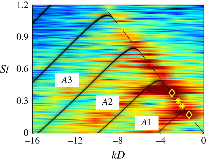
. The spectrum calculated on the jet axis is represented in figure 24 as a function of the Strouhal number and the wavenumber. Only the negative wavenumber part of the spectrum is shown. Significantly levels are found along bands resembling the dispersion relations of the axisymmetric acoustic wave modes
 $A1$
,
 $A2$
and
 $A3$
of a jet at
 ${\mathcal{M}}_{j}=1.5$
, which are also plotted in the figure. These bands are slightly above the theoretical curves, which is likely due to the hypothesis of an infinitely thin shear layer in the vortex-sheet model, as discussed in the Appendix. Strong levels also appear along the line
 $k=-\unicode[STIX]{x1D714}/a_{0}$
at specific frequencies, in particular at the tone Strouhal numbers
 $St_{1}$
and
 $St_{4}$
associated with axisymmetric jet oscillations. On the contrary, the levels are weak at the tone Strouhal numbers
 $St_{2}$
and
 $St_{3}$
associated with helical oscillations, as expected on the jet axis.
Frequency–wavenumber spectrum of pressure fluctuations on the jet axis between
 $z=0$
and
 $z=L-2r_{0}$
for JetL12; —— dispersion relations of the axisymmetric neutral acoustic wave modes for an ideally expanded round jet at
 ${\mathcal{M}}_{j}=1.5$
; – – –
 $k=-\unicode[STIX]{x1D714}/a_{0}$
; LES tone frequencies associated with ♢ axisymmetric and * helical modes. The colour scale levels spread over 30 dB from blue to red.

The pressure spectra determined at
 $r=r_{0}$
for JetL12 for the azimuthal modes
 $n=0$
and
 $n=1$
are represented in figure 25 as a function of the Strouhal number and the wavenumber. The levels are lower than on the jet axis, which is in line with the eigenfunction distributions of the neutral acoustic wave modes (Tam & Ahuja Reference Tam and Ahuja1990). However, as previously, peak levels are reached along the line
 $k=-\unicode[STIX]{x1D714}/a_{0}$
at the tone Strouhal numbers
 $St_{1}$
and
 $St_{4}$
in figure 25(a) and
 $St_{2}$
and
 $St_{3}$
in figure 25(b). Therefore, at the frequencies of the axisymmetric and helical tones, there exist axisymmetric and helical waves, respectively, which propagate in the shear layers in the upstream direction at the phase speed
 $a_{0}$
. These waves are very likely to close the feedback loop just downstream of the nozzle exit, thus exciting the instability waves observed in the shear-layer velocity spectra of figure 8.
Frequency–wavenumber spectra of pressure fluctuations at
 $r=r_{0}$
between
 $z=0$
and
 $z=L-2r_{0}$
for JetL12 for the azimuthal modes (a)
 $n=0$
and (b)
 $n=1$
;
—— dispersion relations of the axisymmetric neutral acoustic wave modes for an ideally expanded round jet at
 ${\mathcal{M}}_{j}=1.5$
; – – –
 $k=-\unicode[STIX]{x1D714}/a_{0}$
; and LES tone frequencies associated with ♢ axisymmetric and * helical modes. The colour scale levels spread over 30 dB from blue to red, with a
 $-6$
dB shift compared to figure 24.

4 Conclusion
In this paper, the production of tones by ideally expanded supersonic round jets at a Mach number of 1.5 and a Reynolds number of
 $6\times 10^{4}$
impinging on a flat plate at four distances from the nozzle between 6 and 12 nozzle radii has been investigated. With this aim in view, the results of large-eddy simulations and of different models of the aeroacoustic feedback mechanism responsible for the tones are compared. Upwind-propagating acoustic waves probably closing the feedback loop are also detected in the simulated jets, for the first time to the best of our knowledge for a supersonic jet flow.
In a first step, the main characteristics of the flow fields obtained by LES, including velocity spectra and convection velocity in the shear layers, are presented. The near pressure fields are then explored using Fourier transform. Standing-wave patterns and axisymmetric or helical oscillation modes are observed at the tone frequencies. In a second step, the predictions obtained from the classical feedback model, in which the feedback loop is closed by acoustic waves travelling outside the jets, and those provided by an analysis of the upstream-propagating subsonic acoustic wave modes of the jets are shown. Overall, they are in fair agreement with the LES data. More interestingly, it is found that combining the feedback model and the wave analysis allows us to determine the tone frequencies, the mode number of the feedback loop, and the axisymmetric or helical nature of the jet oscillation modes, but also the probability of the tones to emerge. Indeed, a tone at a certain frequency appears likely to be generated when at this frequency there exists, based on the wave analysis, upstream-propagating acoustic waves with a group velocity and a phase velocity very close to the ambient sound speed. Such waves are clearly identified in the flow fields of the present ideally expanded impinging jets, and characterized using frequency–wavenumber spectra of pressure along the jet axis and the nozzle lip line. These results suggest that the feedback loop is closed by acoustic (instability) waves of the jets travelling upstream at the ambient speed of sound inside the flow, but also outside for supersonic jets (Tam & Ahuja Reference Tam and Ahuja1990).
Acknowledgements
This work was granted access to the High-Performance-Computing resources of FLMSN (Fédération Lyonnaise de Modélisation et Sciences Numériques), partner of EQUIPEX EQUIP@MESO, and of CINES (Centre Informatique National de l’Enseignement Supérieur), and IDRIS (Institut du Développement et des Ressources en Informatique Scientifique) under the allocation 2016-2a0204 made by GENCI (Grand Equipement National de Calcul Intensif). It was performed within the framework of the Labex CeLyA of Université de Lyon, operated by the French National Research Agency (grant no. ANR-10-LABX-0060/ANR-11-IDEX-0007).
Supplementary movie
A supplementary movie is available at https://doi.org/10.1017/jfm.2017.334.
Appendix
In order to examine the influence of the thickness of the jet mixing layer on the dispersion relations of the upwind-propagating acoustic wave modes, the results provided by the simulations of two temporally developing axisymmetric mixing layers are presented in this appendix. The mixing layers are characterized by the same conditions as the jet considered in this paper, including a Mach number of 1.5 and a Reynolds number of
 $6\times 10^{4}$
. They are initially defined by hyperbolic-tangent velocity profiles of momentum thicknesses equal to
 $\unicode[STIX]{x1D6FF}_{\unicode[STIX]{x1D703}}=0.016r_{0}$
and
 $\unicode[STIX]{x1D6FF}_{\unicode[STIX]{x1D703}}=0.12r_{0}$
. These values corresponds to those measured in the present impinging jets, respectively, at
 $z=0$
and farther downstream at
 $z\simeq 5r_{0}$
, that is, at the nozzle exit and approximately midway between the nozzle and the flat plate for JetL10 and JetL12, refer to figure 5(b). Random pressure fluctuations of a maximum amplitude of 1 Pa are also added at time
 $t=0$
in the jets for
 $r\leqslant 0.5r_{0}$
in order to excite the jet acoustic wave modes.
The numerical framework is identical to that used in the recent computations of a temporal subsonic round jet (Bogey Reference Bogey2017). The simulations are performed using a cylindrical grid extending up to
 $z=500r_{0}$
in the axial direction and out to
 $r=10r_{0}$
in the radial direction. The grid contains
 $n_{r}\times n_{\unicode[STIX]{x1D703}}\times n_{z}=279\times 256\times 20\,000$
points, yielding, in particular, a mesh size of
 $\unicode[STIX]{x0394}z=0.025r_{0}$
in the axial direction. The total number of iterations is equal to 815 for
 $\unicode[STIX]{x1D6FF}_{\unicode[STIX]{x1D703}}=0.016r_{0}$
and 1950 for
 $\unicode[STIX]{x1D6FF}_{\unicode[STIX]{x1D703}}=0.12r_{0}$
, allowing us to reach a final time of
 $t=6.25r_{0}/u_{j}$
in the first case and
 $t=15r_{0}/u_{j}$
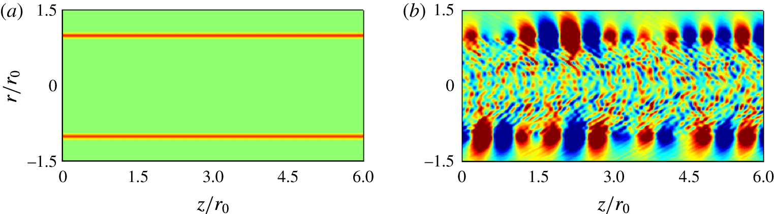
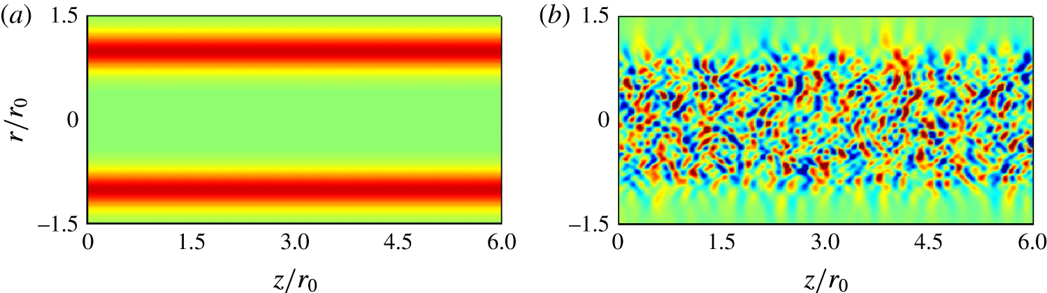
in the second case. At that times, given the weak initial forcing of the jet flow, the mixing layers are still laminar, as illustrated by the vorticity fields of figures 26(a) and 27(a). Instability waves are however visible in the pressure fields of figures 26(b) and 27(b). They consist of Kelvin–Helmholtz instability waves in the mixing layers, and of pressure waves confined inside the supersonic jet core. The latter are the waves of interest here.
Representation of (a) vorticity norm and (b) pressure fluctuations
 $p-\langle p\rangle$
obtained at
 $t=6.25r_{0}/u_{j}$
for the mixing layer of momentum thickness
 $\unicode[STIX]{x1D6FF}_{\unicode[STIX]{x1D703}}=0.016r_{0}$
. The colour scales range up to
 $-18.75\times r_{0}/u_{j}$
for vorticity, and from
 $-0.04$
up to 0.04 Pa for pressure.

Representation of (a) vorticity norm and (b) pressure fluctuations
 $p-\langle p\rangle$
obtained at
 $t=15r_{0}/u_{j}$
for the mixing layer of momentum thickness
 $\unicode[STIX]{x1D6FF}_{\unicode[STIX]{x1D703}}=0.12r_{0}$
. The colour scales range up to
 $-2.5\times r_{0}/u_{j}$
for vorticity, and from
 $-0.04$
up to 0.04 Pa for pressure.

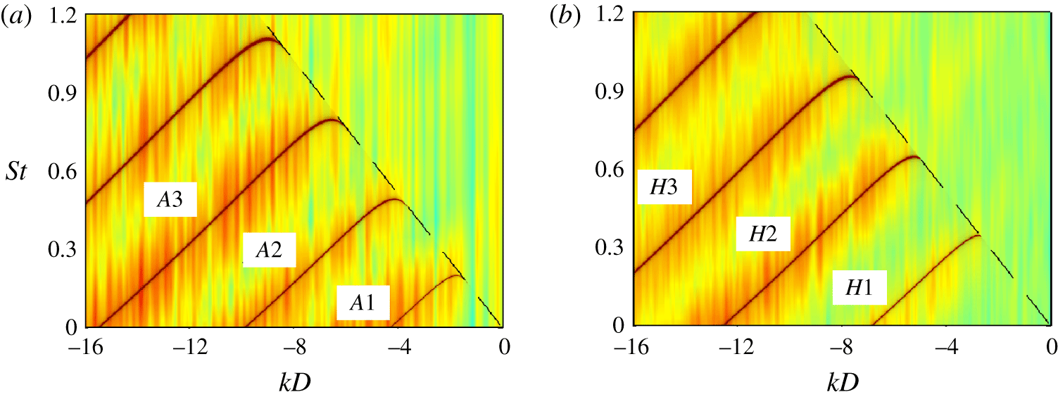
Frequency–wavenumber spectra of pressure fluctuations in a temporal axisymmetric mixing layer of initial momentum thickness
 $\unicode[STIX]{x1D6FF}_{\unicode[STIX]{x1D703}}=0.016r_{0}$
for the azimuthal modes (a)
 $n=0$
and (b)
 $n=1$
;
—— dispersion relations of the axisymmetric neutral acoustic wave modes for an ideally expanded round jet at
 ${\mathcal{M}}_{j}=1.5$
; – – –
 $k=-\unicode[STIX]{x1D714}/a_{0}$
. The colour scale levels spread over 30 dB from blue to red.

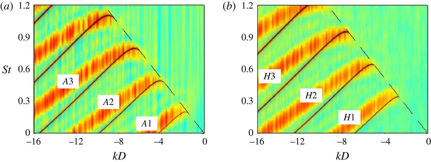
Frequency–wavenumber spectra of pressure fluctuations in a temporal axisymmetric mixing layer of initial momentum thickness
 $\unicode[STIX]{x1D6FF}_{\unicode[STIX]{x1D703}}=0.12r_{0}$
for the azimuthal modes (a)
 $n=0$
and (b)
 $n=1$
; same lines as and colour scale range 7 dB lower than in figure 28.

A space–time Fourier transform has been applied to the pressure fluctuations on the lines at
 $r=0$
,
 $0.1r_{0}$
,
 $0.2r_{0}$
,
 $0.3r_{0}$
,
 $0.4r_{0}$
and
 $0.5r_{0}$
. In time, the Fourier transform is performed using the full signals from
 $t=0$
to
 $t=6.25r_{0}/u_{j}$
for
 $\unicode[STIX]{x1D6FF}_{\unicode[STIX]{x1D703}}=0.016r_{0}$
and from
 $t=0$
to
 $t=15r_{0}/u_{j}$
for
 $\unicode[STIX]{x1D6FF}_{\unicode[STIX]{x1D703}}=0.12r_{0}$
, without windowing function. The spectra obtained for the azimuthal modes
 $n=0$
and
 $n=1$
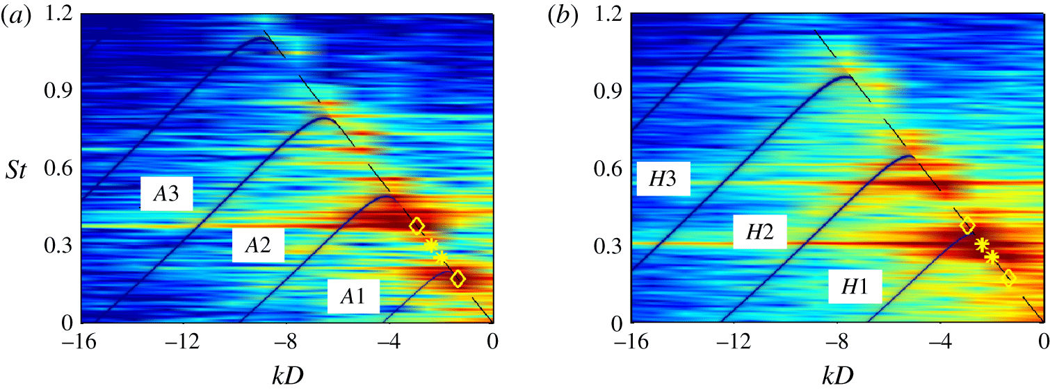
by averaging the results at the six radial locations are represented in figures 28 and 29 as functions of the Strouhal number and the wavenumber. Only the negative wavenumber part of the spectra are shown. The dispersion relations of the acoustic neutral wave modes determined using the vortex-sheet model for a jet at
 ${\mathcal{M}}_{j}=1.5$
are also displayed. For the temporal jet with
 $\unicode[STIX]{x1D6FF}_{\unicode[STIX]{x1D703}}=0.016r_{0}$
in figure 28, despite the very short duration of the pressure signal, significant levels are found along bands centred around the theoretical dispersion relation curves. The use of the vortex-sheet model thus appears well appropriate in this case. For the temporal jet with
 $\unicode[STIX]{x1D6FF}_{\unicode[STIX]{x1D703}}=0.12r_{0}$
in figure 29, the bands given by the simulation are slightly above the theoretical curves, especially for wavenumbers
 $kD<-10$
. These results are consistent with the findings of Tam & Ahuja (Reference Tam and Ahuja1990) for a jet at
 ${\mathcal{M}}_{j}=0.8$
. Above all, they are very similar to those observed in figure 24 for JetL12, which is not surprising given that
 $\unicode[STIX]{x1D6FF}_{\unicode[STIX]{x1D703}}=0.12r_{0}$
corresponds roughly to the mean shear-layer thickness between the nozzle exit and the flat plate in JetL12. The vortex-sheet model however remains a good first approximation in that case.