A standard tenet of economics is that globalization, or the integration of world commodity and factor markets, has profound and predictable effects upon an economy's output mix, resource allocation, and income distribution. To study globalization and its effects, economists construct general equilibrium models that tell the story of the domestic impact of market integration.Footnote 1 Yet no economic historian has employed general equilibrium techniques to study the development of the Roman imperial economy. Sparse data and uncertainty over the degree of imperial market integration and Romans' economic rationalism make the application of traditional models difficult.Footnote 2 While acknowledging these limitations, this article employs a general equilibrium model to tell a coherent story of Italian peninsular development during Rome's expansion from 200 bc to ad 100. The novelty of this approach is the use of a formalized economic model to portray a broad picture of Italian economic development, and the purpose, beyond addressing questions of Roman history, is to argue that constructing such models is a powerful method of studying ancient history.
Historians make valid arguments that Rome's economic expansion had muted effects on the Italian economy, because subsistence farmers did not respond to market incentives and because Romans were motivated more by cultural and social factors than by economics.Footnote 3 In addition, historians contend that it is a mistake to project modern theories onto past societies that functioned in fundamentally different ways.Footnote 4 Economic historians have dedicated much of their recent work, however, to challenging these ideas for ancient Rome and for other places.Footnote 5 For example, some scholars argue that Romans displayed economic rationality in their management of landed estates and in their decisions about migration.Footnote 6
Another controversial debate focuses on the importance of markets in Roman life and the extent to which imperial markets functioned as a “single economic unit.”Footnote 7 Whereas some historians argue that the imperial economy was neither integrated nor reliant upon markets for the fulfillment of needs, others conclude that the market system was an important, if not the dominant, mode of exchange in the empire.Footnote 8 Although he accepts that markets worked slowly and imperfectly, Peter Temin catalogues the widespread use of prices across the empire and concludes that Roman provinces “functioned as part of a single comprehensive Mediterranean market.”Footnote 9
Approaching these debates directly requires knowing what Roman citizens were thinking or a more comprehensive knowledge of their interactions than the contradictory snippets that we possess today. Rather than speak directly to these debates, I develop and then formalize a conceptual understanding of the Italian economy based on the assumptions of perfect economic rationality and market integration. The consistency (or lack thereof) of the resulting predictions and the historical evidence provides an assessment of the model's assumptions and thus indirectly addresses the debates described above. In addition, the model provides a single, coherent view of Italian economic development that addresses many of the questions on which existing models and explanations are singularly focused. The success of the model in predicting what we know of Italian economic history supports the predictions on more controversial questions, the assumptions of economic rationality and market integration that underlay the model, and the approach itself. Of course, constructing a model is an iterative process and the model presented here is basic and oversimplified. My aim, however, is only to convince readers that this approach to ancient history has enough potential to merit the development of more refined and applicable models.
Economic historians have yet to employ general equilibrium models in the study of the ancient past, probably because the limited and uncertain data make the precise predictions possible in studies of the more recent past unattainable. More important than precise predictions, however, is the broad picture of the Italian economy and its development that our economic reasoning and the available evidence convey. The lack of documentation from ancient Rome makes the available evidence a diverse array of archaeological findings, primary sources and government records, demographic and other models, and studies of more recent agricultural economies. Together with the application of economic logic, these fragments provide a picture of the past.
A GENERAL EQUILIBRIUM MODEL OF ROME
The general equilibrium model presented here is an integrated collection of commodity and factor markets driven by supply and demand and together representing the entirety of the Italian economy. The model requires several simplifying assumption that are typical of general equilibrium analysis and will be described in what follows.Footnote 10 The model's inputs are the exogenous variables, such as factor endowments and tradable commodity prices, determined in the empire as a whole and independent of the Italian economy itself. By understanding the cause-and-effect relationships in the Italian economy and establishing how the exogenous variables evolved over time as a result of imperial expansion, one can measure the effects of expansion on the model's endogenous outputs, including the prices of tradable goods and resource inputs and the quantities of resources dedicated to each sector.
My model of the Roman economy consists of three main factors of production—land, labor, and slaves—and four final goods sectors—grain, wine, livestock, and urban goods. Two intermediate goods, feed and manure, provide realistic links between final goods sectors. The model also includes the annona, free grain provided to the populace of Rome by the imperial government. Finally, taxes expropriated from the provinces close the model and finance Italy's trade deficit.
Grain, wine, urban production, and livestock reflect the main sectors of the economy, making the model simple but realistic. Grain, the primary commodity in the subsistence-based imperial economy, and wine, the primary luxury good, constituted 85 percent of the agriculture in cultivable areas.Footnote 11 Livestock was prevalent further from cities in Italy's higher altitude pastureland.Footnote 12 Urban goods, which represent all production in cities and towns including pottery, cloth, furniture, glassware, ironware, and other metal products, help differentiate urban and rural populations.Footnote 13 Although grain, wine, and urban goods were traded over long distances, the lack of refrigeration and the high cost of land transport made trade in livestock between Italy and the rest of the empire prohibitive.Footnote 14 Transported “by the hoof,” Italian livestock was delivered to nearby towns for local consumption.Footnote 15
Thus, livestock prices are not tradable and determined within the model itself, whereas grain, wine, and urban goods prices are tradable and determined in imperial markets. This assumes that Italy was small compared to the imperial economy as a whole and did not impact prices determined in imperial markets. In fact, Italy was a significant imperial market, housing five of its 50 million people and possessing much of its wealth.Footnote 16 Though I consider the impact of domestic markets in understanding grain and wine prices, I leave the small open economy assumption in place to simplify the model.
The model also assumes that factor endowments of labor, slaves, and land were exogenous to the Italian economy. The quantity of labor was driven primarily by political shocks, such as conscription and colonization; high transportation costs prevented provincials from migrating in large numbers to take advantage of Italian economic prosperity.Footnote 17 Similarly, the quantity of slaves was largely dependent on political shocks, mostly the winning of slaves in wars of conquests fought for territorial expansion or defense.Footnote 18 The quantity of land in use was motivated both by economic forces, primarily the desire to bring new lands under cultivation as the returns to agriculture grew, and by noneconomic forces, namely the pushing of peasants ejected from their old ancestral land to more marginal plots.Footnote 19 Overall, assuming that factor endowments are exogenous is largely consistent with what we know of Italian labor, slaves, and land use at this time and usefully simplifies the model.
Though in later societies slaves and labor are often close substitutes, this model posits a differentiation between free and slave labor and the income shares that they receive from grain and wine production, based on their different characteristics in Roman society.Footnote 20 Slaves worked harder and longer than peasants would tolerate.Footnote 21 Peasant absences to fight wars reduced their reliability and their overall presence on the farm.Footnote 22 Peasants excluded themselves from working on large estates alongside slaves for cultural reasons.Footnote 23 Furthermore, while grain production requires intense labor only during peak season, wine production requires constant and intensive labor throughout the growing season.Footnote 24 For this reason, slave labor, rather than free labor with its frequent absences and more lax work habits, was more profitably employed in wine production. The model captures this understanding by separating free and slave labor and by positing different production functions for grain and wine.
The model includes the annona, or the dole of free grain provided by the imperial government, because it was a significant source of income for urban residents and probably an important psychological factor motivating peasant migration to the capitol. At its peak some 300,000 Roman residents, or 5–10 percent of the Italian population, received the annona, and its prominence in the historical record suggest that its impact on the contentment of the Roman populace was greater than that.Footnote 25 In addition, the prospect of free grain was probably appealing to peasants far from Rome, motivating their migration despite the annona's restriction to only a slice of Roman residents. For the purposes of the model, I assume that the annona was free throughout its existence and distributed evenly among urban residents.
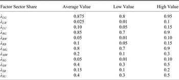
With the model broadly established, I now delve into and describe its parameters, which determine how changes in commodity prices and factor endowments affect commodity and factor prices.Footnote 26 The most important parameters define which and in what proportion the factors of production—labor, slaves, and land—receive income from the production and sale of each commodity. A combination of Roman contemporary agronomist texts, comparisons with later subsistence economies, and knowledge of the agricultural commodities themselves provide us the picture of how commodity revenues were split. What matters here are not exact figures but the overall picture of how resources combine to generate output.
Grain production requires a combination of free labor and land with small additions of slaves and manure. Roman peasants tended to produce grain rather than wine for the reasons described previously.Footnote 27 Agronomist texts and research on grain production in later periods largely corroborate this picture and add information on how agricultural output is divided amongst the labor force and landowners.Footnote 28
Wine production, on the other hand, intensively demands slaves and largely excludes the other factors of production. Wine's dependence on slaves over free labor is described above, and its labor intensiveness and high value over land density make slaves more important than land as well. Agronomist texts educating contemporary Roman farmers on their vineyards paint a picture of wine production from which we can infer the share of each factor of production in wine output.Footnote 29
Urban goods are produced by some combination of free labor and slaves. As no data exist on their relative importance, I assume that free labor and slaves shared the output of urban production evenly. Finally, livestock production intensively employs land and feed and requires relatively little labor. As limited data exist for Rome, I apply Kevin O'Rourke's findings on livestock's factor income shares in pre-industrial Ireland to the Roman economy.Footnote 30
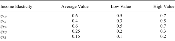
Other parameters are the initial conditions of the Roman economy and the income elasticities of free labor, landowners, and slave owners, to whom all slave income accrues. The initial conditions describe an Italian economy dominated by grain production but lacking in wine, urban, and livestock production, and abundant in labor and land but scarce in slaves.Footnote 31 Income elasticities define how each factor of production spends the money it earns and thus affects how incomes are redirected to the consumption of other goods. Free labor primarily spends its money on subsistence and then spends small portions on other goods once subsistence requirements are satisfied.Footnote 32 Landlords and slave owners spend their incomes on wine, urban goods, and livestock, reflecting their greater wealth spent on luxuries and the ease with which they covered their subsistence needs.Footnote 33
More detailed parameter specifications and explanations are included in the Appendix. Given the imprecise nature of the data, I examine the model's output for a broad range of parameters.
IMPERIAL EXPANSION AND THE EXOGENOUS SHOCKS TO THE ITALIAN ECONOMY
Imperial expansion affected the nature of the Italian economy in powerful ways. My model explains how the direct effects of expansion, or the exogenous shocks to the Italian economy, affected the decisions of economic actors and caused ripples throughout the economy. To study their consequences, we must first understand more completely the shocks to the Italian economy and the degree of certainty and precision with which we know them.Footnote 34 First I describe those that we know more confidently—the rise in the slave population, the expansion of land under cultivation, the decline in free labor, and growth of the annona—before addressing those that are more uncertain—the ambiguous change in grain prices and the rise in wine and urban goods prices. Throughout, I describe both the underlying cause-and-effect relationships that drive these changes and the available data.
The exogenous shock to the Italian economy most apparent in the historical record is the tremendous growth of the slave population after 200 bc. The constant influx of slaves from provincial wars more than offset slaves' high death rates and high rates of manumission and in fact accounted for virtually all of Italy's population growth during this period.Footnote 35 Historians estimate that Italy's slave population was roughly 500,000 in 200 bc. Estimates of Italy's slave population 200 years later, based on war and economic records cataloguing slaves won from victories and trades, range from 1.2 to 2 million people, or up to 30 percent of Italy's total population.Footnote 36 Examining the estimates, I have most confidence in Walter Scheidel's detailed analysis of the demographic factors affecting the slave population, which leads him to a conservative estimate of 1.2 million slaves in 1 bc.Footnote 37 Of course, the precise figures based on historians' calculations are unimportant; what matters is the clear growth in the Italian slave population by a factor of two or more.
It is also fairly well established that the free population of Italy stayed constant or declined slightly after 200 bc. A balance of natural reproduction against death rates, conscription, and colonization of the provinces determined the path of Italian population growth.Footnote 38 Though we do not know whether the population remained constant or fell, it is clear that the burden of imperial expansion, which required that free peasants serve in the army and populate foreign provinces, was a significant drain on the free labor population and stymied any material population gain. Most estimates point to a modest decline by 1 bc as the drain of imperial expansion overwhelmed natural reproduction.Footnote 39
The expansion of land under cultivation during this period clearly follows from our knowledge of Italian development, though little reliable evidence exists to support the claim. Gains in total population and the opening of provincial markets raised the returns of agriculture, making marginal lands profitable and motivating wealthier land and slave owners to push peasants to those marginal lands.Footnote 40 The recovery of Italy from the Hannibalic War in the late third century bc also contributed to growth in land use.Footnote 41 Based on the number of soldiers, the size of plots, and the degree to which these settlements did not disturb existing landholders, the practice of granting soldiers settlement rights after wars by itself expanded land under cultivation by 5 percent.Footnote 42 Though the archaeological record provides evidence of expansion at this time, the lack of preserved remains from the prior period does not necessarily indicate that areas were uninhabited.Footnote 43 However, the major factors driving the use of land all point to greater land use after 200 bc, and, though the data are lacking, an expansion in land under cultivation probably occurred.
The prominence of the annona in the historical record allows us to precisely quantify its growth. Originally, the Senate sold up to 40 modii of grain to about 50,000 Roman residents at a cost of HS 1.5 per modius. By 54 bc, the annona provided 40 modii of free grain to nearly 300,000 Roman citizens, a number later reduced to 200,000.Footnote 44
The evolution of commodity prices after 200 bc is less clear than the more established changes in the slave and free labor populations, the degree of land use, and the annona. The lack of consistent price data makes any conclusions drawn from price comparisons tentative. However, an examination of the evidence suggests that there was a significant expansion in trade throughout the empire, contributing to both strong correlations between commodity prices in Italy and the provinces and convergence between Italian and provincial prices. After 200 bc, the creation of provinces, the dispersion of the military and coinage, the construction of roads and canals, and the pacifying of the Mediterranean, among other factors, led to a substantial growth in imperial trade.Footnote 45 Shipwreck data display a threefold rise in the number of shipwrecks, a proxy for the number of voyages, from the third century bc to the first century bc.Footnote 46 The growth of the money supply, which was used especially for long-distance exchanges, suggests a significant expansion in the quantity of traded goods.Footnote 47 By the first century ad, commodity prices in Italy and in the provinces were highly correlated. For example, David Kessler finds a significant correlation between Egyptian and Italian prices, with Italian prices responding to shocks in Egypt in a predictable manner.Footnote 48 In his analysis of supplying the city of Rome, Geoffrey Rickman concludes that “the situation in Rome was. . . [that] the local resources were not so relevant by the period of early Empire. . . What affected the Roman market more was first the failure of harvests in provinces overseas. . .; secondly, inadequate supplies of shipping, and the destruction of corn ships in storms at seas . . .”Footnote 49
In addition, the growth of trade suggests that commodity prices in Italy and the provinces were converging. Imperial markets, primarily Egypt and North Africa, accounted for 50–75 percent of grain imports to Rome and at least 25 percent of demand for Italian wine.Footnote 50 This suggests that imperial expansion led to an influx of provincial grain, depressing Italian grain prices; provided new markets for wine, raising Italian wine prices; and caused grain and wine prices in Italy and its provinces to converge. Indeed, according to Kessler, 90 percent of the grain price differential between Egypt and Italy was due to transportation costs by the first century ad.Footnote 51 In the language of classical economic theory, Italy had a comparative advantage in wine and urban goods production (because they employed intensively what Italy possessed in abundance, slaves and an urban labor force) and a comparative disadvantage in grain (because grain employed intensively what Italy possessed in scarcity, land).
With this broad picture established, I now examine the factors affecting commodity prices and the available data in more detail. Economic forces pulled Italy's grain prices in opposite directions. The opening of the provinces substantially expanded the supply of grain reaching Italian markets and placed downward pressure on grain prices. Meanwhile, domestic factors, primarily the growth in Italy's total population, increased demand, and the conversion of resources from producing grain to other goods reduced Italian supply, pushing prices higher. The path of grain prices becomes an empirical question on which the data are inconclusive.Footnote 52 For the purposes of the model, I follow the small open economy assumption and hold that grain prices fell. However, the model's results are consistent across a range of grain price changes, including constant prices and moderate price growth.
Unlike the case of grain, economic forces unambiguously pressured wine and urban goods prices higher. After 200 bc, both wine and urban goods faced greater demand from the rest of the empire and from domestic consumers.Footnote 53 Whereas the data tentatively indicate that wine prices rose over our period, the data on urban goods prices are non-existent.Footnote 54
Our understanding of directional changes and approximate magnitudes is sufficient to draw logical conclusions about the development of the Italian economy from our conceptual framework of how the Italian economy worked. The following sections address the predictions of the model—first those that are consistent with existing evidence to establish the model's credibility and then those that address more controversial issues.
RESULTS AND INTERPRETATION
What, then, does the model predict?Footnote 55 The model's results turn out to be consistent across a broad range of plausible parameter values and exogenous inputs. Moreover, the model's directional predictions are largely consistent with the available evidence. On the other hand, the model's predictions of magnitude generally overshoot the historical reality, thus exposing the flaws in our assumptions of an Italian small open economy, perfect markets and economic rationality.
Nonetheless, the model's success in predicting known economic developments in Italy after 200 bc lend credence to its implications for more controversial questions. Among its comforting successes are two major, well-documented developments in the Italian economy after 200 bc: the shift from grain to wine production in the countryside and the migration of free labor from rural to urban areas. The model also makes more controversial predictions: peasants migrate mostly due to pull factors and not push factors; slave owners gain from imperial expansion while landowners lose; and the bulk of Italian wealth derives from the expropriation of resources and people from the provinces.
First among the predictions that lend credence to the model is the shift from grain to wine production in the Italian countryside, though the model overestimates the degree of this transition.Footnote 56 In the model, the rise in wine prices relative to grain prices makes wine more profitable than grain. The growth in slaves relative to land and free labor makes slaves cheaper and wine production relatively less expensive. In response Romans redirect resources from grain to wine production, and Italy exports its wine surplus and imports its grain shortage.Footnote 57
The archaeological evidence of Italian trade with the provinces and land use and contemporary Roman accounts support this story. Grain imports to Italy grew from five million modii per year in 200 bc to 30–60 million modii per year by 1 bc.Footnote 58 Wine exports also peaked at this time; the excavation of amphorae, or wine containers, reveal significant Italian wine exports to Gaul that declined over the subsequent centuries.Footnote 59 Shipwreck data also show that over half of shipwrecks on shipping routes from Italy to Gaul occurred in the second and first centuries bc.Footnote 60 Examining the Italian countryside, archaeological digs throughout Campania and Etruria indicate a proliferation of wine-producing villa sites through the first century bc, with 22 percent of land in Etruria and 15 percent of land near Pompeii dedicated to wine production.Footnote 61 The largest, most elaborate villas were inhabited in roughly the same 100 year period that corresponds with the growth, peak, and decline of the Italian wine industry. Contemporary Romans were aware of these changes. As Pliny the Elder writes, “Then come the favoured country of Campania; in this valley begins those vine clad hills with their glorious wine. . . famous all the world over, and. . . the scene of the severest com-petition between Father Liber [wine] and Father Ceres [grain]. . . .”Footnote 62
A second major prediction of the model is a significant migration of free labor from rural to urban areas.Footnote 63 In the model, a combination of rising urban goods prices, the expansion of the annona, and falling grain prices makes city life more attractive than country life, while higher returns to wine production motivate landowners to push peasants off their lands and convert them into villa estates. Although the question of why peasants migrated remains controversial, the mass migration of peasants predicted by the model is well established. Based on city and town remains and contemporary written records, historians estimate that the peninsula's urban population grew from 500,000 in 200 bc to 1.2 million two centuries later.Footnote 64 Using estimates of urban death rates, Scheidel calculates that rapid urbanization absorbed 1.8 to 2.2 million peasants between 200 and 1 bc. The mass migration of peasants from the hinterland to Rome and other cities was a phenomenon not seen again in Western history until London's boom more than a millennium later.
In two major areas, the model's implications are consistent with the evidence, although the predicted magnitudes overestimate the historical reality. What, then, does it say about the more controversial and unknown questions of why peasants migrated, who gained and who lost, and how Italy became wealthy? Many existing theories about why peasants migrated emphasize that profit-hungry aristocrats and low grain prices pushed peasants from their land and that imperial expansion left ordinary Romans destitute by the first century ad.Footnote 65 More recent theories, less prevalent in the literature, suggest that pull factors, notably opportunities in cities and towns, inspired most urban migration.Footnote 66 The model can speak to the question by allowing us to estimate the fraction of the shift from grain to urban production driven by push and pull factors. According to the model, pull factors, primarily the rise in urban goods prices and the expansion of the annona, drive 80 percent of peasant migration after 200 bc.
Scheidel's recent demographic analysis lends support to this conclusion. The variations of the push theory focus on peasant dislocation in the second century bc, either as a result of Hannibal's pillaging of the Italian countryside, falling grain prices, or constant militarization of the peasantry.Footnote 67 By contrast, pull theories focus on growing opportunities, such as the rise of the annona and Italian urban production, which became more prevalent in the first century bc and afterwards.Footnote 68 Scheidel's analysis shows that growing Italian cities required an increasing supply of immigrants to replenish their populations because urban death rates exceeded birth rates, a conclusion more consistent with the timing of pull theories than push theories.Footnote 69 Scheidel's analysis favors pull theories of migration over the push theories and casts doubt on theories that imperial expansion impoverished Roman peasants by driving them from their lands.
The literature is unclear on who gained and who lost from imperial expansion, though it is generally agreed that peasants lost while aristocrats gained. Our model, however, tells a different story. It acknowledges that falling grain prices reduce free labor's real income because most laborers were employed in grain production. This is almost entirely offset, however, by growing opportunities in urban areas and the expansion of the annona, for a minimal net effect on free labor income.Footnote 70 The model's story thus contradicts those who believe that peasants were made destitute by falling grain prices, evictions, and slave imports. But it fits Peter Garnsey's conclusion that peasant livelihoods remained unaffected by imperial expansion, although for different reasons. Whereas Garnsey believes that peasants continued to farm their smallholdings undisturbed, the model predicts that peasants maintained their incomes only by responding to changing economic conditions and moving to urban areas.Footnote 71 The massive migration of free labor from the countryside to cities and towns—around two million peasants over 200 years, at approximately the same rate as English peasant migration in the nineteenth century—suggests that the model's story is more accurate.Footnote 72
Overall, the model tells a more complex story about land and slave owners. Landowners lose while slave owners gain, as falling grain prices and more scarce free labor make grain production less profitable and rising wine prices and more abundant slaves make wine production more lucrative. Wealth thus shifts to aristocrats wealthy enough to own slaves at the expense of middling landowners who cannot afford slaves and for whom selling their lands and migrating to cities is an unappealing option.Footnote 73 Projecting these predictions onto the past, aristocrats' incomes would have declined in the second century bc, as grain prices fell, only to rise again to new heights as wine production flourished.
There is some evidence of trouble for Roman landowners in the second century bc and substantial evidence for high and climbing returns to owning slaves. Landlords' ability to purchase large plots of land in the second century suggests depressed prices at that time.Footnote 74 The decline in the structure and size of rural residences and the depopulation of productive areas indicate that formerly wealthy aristocrats had fallen on hard times.Footnote 75 On the other hand, the price of slaves, or the present value of slave returns, grew significantly during this period. A catalogue of the prices slaves paid for their freedom at Delphi indicates a 50 percent gain in slave prices, or the present value of slave returns, after 200 bc.Footnote 76 Mentions of slave prices in contemporary sources, including Livy and Tacitus, suggest an eight- to tenfold gain in slave prices between 200 bc and ad 200.Footnote 77
As the wine industry flourished and the returns to slave owning grew, slave owners accumulated enormous and unprecedented fortunes. Richard Duncan-Jones's catalogue of Roman private fortunes reveals that the number of Romans with more than HS 200 million grew sixfold by the early imperial era.Footnote 78 Sites in Latium and Campania became larger, more common, and of much higher quality construction and decoration after 100 bc, and praise of magnificent villas in these areas replaced descriptions of fertile grain lands.Footnote 79 Indeed, the first century bc witnessed the construction of more elaborate and finer villas than ever before.Footnote 80
As slave owners became wealthier Roman society became immensely unequal, a reality evident at the time. Seneca compares the unimpressive size of the residence of general and consul Scipio Africanus, circa 200 bc, to those of his own day in the first century ad.Footnote 81 Livy comments that the wealth requirements for Senate membership doubled during this period.Footnote 82 A calculation of Gini coefficients based on Livy's figures suggest that the Gini coefficient of the Italian population rose from 0.11 in the second century bc to 0.23 100 years later. Indeed, the average senator generated 200 times more income than a peasant's subsistence wages in the early imperium.Footnote 83 Roman fortunes of HS 400 million surpassed sixteenth- and seventeenth-century English totals by a factor of 18–72 in wheat equivalent, and Gini coefficients of Roman landownership compare to British figures from the early modern age.Footnote 84 The model also provides an explanation why and how this occurred—not through the exploitation of peasants, but through the importing of vast quantities of slaves and the opening of new provincial markets for slave-intensive production.
Finally, the model addresses the question of the sources of Roman wealth after 200 bc. In the model Roman wealth derives from two potential sources—the expropriation of provincial wealth, including grain and slaves, and the gains from the market economy. Although the literature often describes Rome's seizure of vast quantities of provincial wealth in the form of tribute and slaves, the questions of how much Italy gained and whether its gains derived from expropriation or markets are hardly addressed.Footnote 85 The model predicts that Italy's total factor income rises 25 percent during this period: 5 percent from market integration and 20 percent from seizures of wealth and people.Footnote 86 In other words, the Italian economy's expansion is driven primarily by the expropriation of provincial wealth, but also significantly by gains from trade. The prediction only provokes further questions, as few data exist to corroborate or deny this interpretation.
That the model's story fit the historical evidence in two well-established aspects of Italian development—the rural transition from grain to wine production and the migration of peasants to cities and towns—makes its more controversial predictions plausible. These controversial predictions find support in the historical evidence as well. The model's success also lends credence to its assumptions of a well-integrated market system in the Roman empire and of economic rationality among the Romans. The degree to which the model's predictions of magnitude overshoots observed historical phenomena, however, reveal that its oversimplified assumptions fail to capture the more complex reality of Roman times.
CONCLUSION
In this article I construct a simplified general equilibrium model of the Roman economy, in order to shed light both on the validity of my assumptions and on the big questions of Italian economic development. I proceed to defend and explain the model and to describe the changes exogenous to the model that resulted from Rome's imperial expansion. Although the model's predictions of magnitude tend to overstate observed phenomena, its directional predictions—the conclusions drawn from the underlying logic on which the model is based—tell a broad story of Roman economic development that is confirmed by the available historical evidence. This fit between the model and the available evidence supports the model's other predictions and its assumption of well-integrated imperial markets and Roman economic motivation and rationalism.
Further research can apply such models to study other aspects of ancient history, such as the decline of Italy after the first century ad or the impact of monetary inflation in the later empire, or use them to refine our assumptions about the Roman economy. Imperial markets suffered from immense communication lags and costs not reflected in this model.Footnote 87 Romans were not solely motivated by economics but also by rules-of-thumb, social pressures, and conventions.Footnote 88 They were not pure profit maximizers but instead focused on maintaining their subsistence and reducing their risk of ruin.Footnote 89 Italy was a major part of the Roman economy and probably affected commodity prices throughout the empire. The model's simplified assumptions about these realities make it a useful tool for telling the broad story of Italian economic development but limit its use as a precise predictive tool. Introducing these complexities into the model would make its story a more realistic portrayal of Italian economic development and would refine, but not substantially change, our understanding.
The basic power of a model is its formalization of our understanding of cause and effect relationships. The combination of formalized understanding and the available data allows us to make more powerful predictions than we can make with the available data alone. This makes models a useful for the study of ancient history, where our data are limited. Furthermore, the power of an economic model such as that used here is its crystallization of a coherent story that considers the complex interactions of many simultaneous changes in an economy and delivers a broad series of testable predictions. This quantified story is more comprehensive and more testable than the historical models often focused on single questions in isolation. Despite these advantages, I believe that historians and economists alike have hesitated to employ economic models in their study of the ancient world because the degree of precision that these models typically require is unknowable for that era. However, economic models do not necessitate knowing the precise outline of an economy to tell a basic, coherent, and accurate story. The broad use of economic models in the study of the distant past would make a significant positive impact on our understanding of ancient history.
Appendix: A Computable General Equilibrium Model of Roman Italy
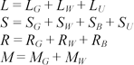
The model has four sectors—grain (G), wine (W), livestock (B), and urban production (U)—and three factors of production—land (R), labor (L), and slaves (S). Two intermediate goods, manure (M) and feed (G B), also function as factor inputs. Manure is produced by livestock and feed consists entirely of grain. The production functions below are Cobb-Douglas in form with constant returns to scale.

In equilibrium, factor markets balance supply, given exogenously, and demand, derived from the sectors in which each factor is employed. Labor demand derives from the grain (L G), wine (L W), and urban (L U) sectors; land from the grain (R G), wine (R W), and livestock (R B) sectors; and slaves from the grain (S G), wine (S W), livestock (S B), and urban (S U) sectors. Manure's supply is given by the production function for manure above and by demand from the grain (M G) and wine (M W) sectors
Commodity markets are supplied by imports and domestic production and demanded by domestic consumers and exports. The grain supply comes from private market imports (G M), government imports for free grain distributions (G A), and Italian production (G). Government imports are determined by the per capita amount of grain distributed (g A) and the urban population (L U). Feed (G B), laborers, and slaves demand grain, with labor and slaves consuming their per capita requirements (g L and g S) multiplied by their total factor endowments (L and S):

where G A = g AL U.
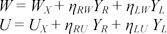
Wine and urban goods are supplied solely by Italian production (W and U) and demanded by exports (W X and U X), landlords, and laborers. Landlords and laborers spend fractions (η RW and η LW on wine and η RU and η LU on urban goods) of their total incomes (Y R and Y L) on wine and urban goods:
Unlike grain, wine, and urban goods, livestock is nontraded. Otherwise the livestock market is similar:

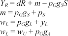
Landlords receive their total income (Y R) from land rents (dR) and the return to slaves (m) minus subsistence costs. At equilibrium slave returns equate to slave costs, which consist of subsistence costs (p Gg S) and price (p S). The nominal wage rate (w L) is spent upon subsistence grain requirements (p Gg L) and other commodities (y L). The nominal urban wage, at equilibrium equivalent to the rural wage, has two components, namely the wage paid by the urban sector (w U) and the income provided by the grain dole (p Gg A):
The final equation is the balance of trade condition, which states that the value of exports equals the value of imports. Export value includes wine exports (p WW X), urban exports (p UU X), and taxes levied upon the provinces (T). Import value includes grain imported by the government (p GG A), grain imported by the private markets (p GG M), and slaves imported from the provinces (p SS):

I solved the model by hand and used Microsoft Excel to examine its results, which are shown in Appendix Tables 1–7.
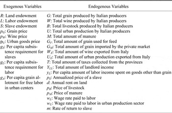
VARIABLE DEFINITIONS

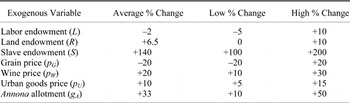
EXOGENOUS SHOCK DIRECTION AND MAGNITUDES

Sources:
See the text.
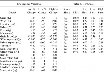
MODEL OUTPUTS

Sources:
See the text and model as specified in the Appendix. I solved the model using Microsoft Excel. The model is based on exogenous shocks, factor income shares, income elasticities, and other initial conditions stated in Appendix Tables 2, 4, 5, 6, and 7, respectively.
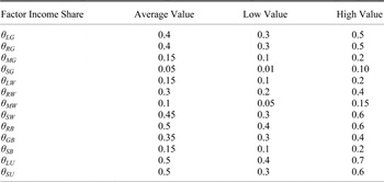
EXOGENOUS FACTOR INCOME SHARES

Note:
A factor income share is the proportion of income derived from the sale of an output that is earned by each factor in its production. For example, the share of total revenue from grain production that the labor producing grain sees as income is labor's factor income share of grain (θLG).
Sources:
See the text.
INITIAL FACTOR SECTOR SHARES

Note:
A factor sector share is the proportion of the factor dedicated to the production of a sector. For example, the proportion of labor dedicated to grain production is the factor sector share of labor with respect to grain (λ LG).
Sources:
See the text.
EXOGENOUS INCOME ELASTICITIES
Note:
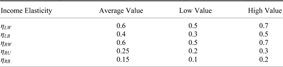
An income elasticity is the fraction of total income spent on each good. For example, the fraction of their total income that landowners spend on wine is the income elasticity of landowners for wine (η RW). The wine and livestock income elasticities of labor are calculated after accounting for labor's grain consumption; the assumption is that laborers spend a fixed amount on grain for subsistence before consuming wine and livestock.
Sources:
See the text.
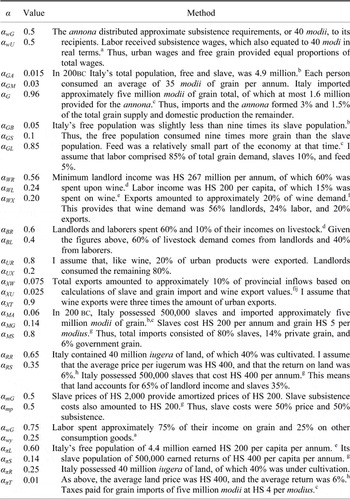
CALCULATION OF OTHER INITIAL CONDITIONS

Note:
This table provides my assumptions on the Italian economy's initial conditions around 200 bc where not already given by factor income shares, factor sector shares, or income elasticities. Included in this table (in order) are the proportion of urban labor's total wages derived from the production of urban goods and the annona; the proportion of grain consumed in Italy originating from Italian farms, grain imports, and the annona; the proportion of each commodity output (grain, wine, livestock, and urban goods) consumed by labor, slaves, landlords, and (for grain) as feed; the proportion of total exports in the form of wine, urban goods, and taxes; the proportion of total imports in the form of the annona, other grain, and slaves; the proportion of landlord income earned from land and slaves; the proportion of slave prices derived from subsistence costs and slave prices; the proportion of labor income spent on grain and other goods; and the proportion of total GDP derived from labor, slaves, land, and taxes.
Sources:
a Garnsey Cities, Peasants and Food, p. 96.
b Brunt Italian Manpower, p. 121.
c Rickman, Corn Supply, pp. 36–42.
d Jongman, Economy and Society, p. 195; and Table 6.
e Garnsey, Cities, Peasants and Food, p. 96; and Table 6.
f Tchernia, “Italian Wine,” p. 92.
g Rickman, Corn Supply, p. 151; and Duncan-Jones, Economy, p. 12.
h Duncan-Jones, Economy, pp. 51–52.
i Garnsey and Saller, Roman Empire.
j Scheidel, “Human Mobility in Roman Italy, 2.”