INTRODUCTION
Australia produced 819 000 t of cotton lint in 2000/01, representing 0·042 of global production (ABARE 2008). However, in 2007/08, cotton production in Australia fell to 132 kt (a reduction of 83·8%) or 0·005 of world production. Reduced cotton production is a result of a decrease in production area (from 527 300 ha in 2000/01 to 62 700 ha in 2007/08), largely as a result of the widespread drought in eastern Australia in recent years (ABARE 2008; CRDC 2009). However, between 2000/01 and 2007/08, the average cotton yield in Australia increased by 36·5%, from 1·6 to 2·1 t/ha (ABARE 2008), due to a marked reduction in dryland cotton farming area and increases in farm inputs with increasing mechanizations. Around 0·65 of Australia's cotton is grown in New South Wales and 0·35 in Queensland (ABARE 2008), due largely to a suitable summer rainfall pattern, soils and topography (CRDC 2009).
The Australian cotton industry is labour-, water- and energy-intensive. Cotton production requires energy for ploughing, applying agrochemicals (fertilizers, herbicides, insecticides, fungicides and plant growth regulators), planting, watering, crop cultivation, harvesting, slashing, stalk pulling and transport. Crop intensification, mechanization and modernization have never been greenhouse gas (GHG) emission-free as they require the use of more fuel, farm machinery and agrochemicals. In addition, production, packaging, transportation and application of agrochemicals in the cotton industry require significant energy resources, resulting in even more GHG emissions (Stout Reference Stout1990; Hülsbergen et al. Reference Hülsbergen, Feil, Biermann, Rathke, Kalk and Diepenbrock2001; Vlek et al. Reference Vlek, Rodriguez-Khul and Sommer2003; Chauhan et al. Reference Chauhan, Mohapatra and Pandey2005; Maraseni et al. Reference Maraseni, Cockfield and Apan2007, Reference Maraseni, Mushtaq and Maroulis2009).
Given that almost all cotton produced in Australia is exported (ABARE 2008), the cotton industry must maintain product quality to remain globally competitive. It must also be efficient in its use of scarce resources and environmentally sustainable. With an increasingly carbon-conscious society and the imminent introduction of the Australian Government's Carbon Pollution Reduction Scheme (CPRS; DCC 2008), the cotton industry (as with other activities in the agricultural sector) needs research to provide accounts for all farm inputs related to GHG emissions. The aim of the present study is to estimate GHG emissions from various cotton farm inputs associated with three common cotton farming systems in the Darling Downs region, one of the major cotton producing regions in Queensland.
Specifically, the present study estimated GHG emissions due to: (1) the production and combustion of fossil fuels used in cotton farm operations; (2) agrochemical production, packaging, storage and transportation; (3) soil-derived nitrous oxide (N2O) from nitrogen (N) fertilizer usage; (4) electricity use in cotton irrigation; and (5) farm machinery production and use in the cotton industry.
Australia's CPRS and the agricultural sector
The Australian Government plans to implement a comprehensive range of climate strategies, which includes mitigation, adaptation and assisting other countries in seeking global solutions. As a mitigation strategy, the Australian Government is committed to reducing Australia's GHG emissions by 5–15% by 2020 and 60% by 2050 below 2000 levels (DCC 2008). To meet these targets in a cost-effective manner, the Australian Government's White Paper (DCC 2008) proposed a comprehensive CPRS, scheduled for implementation in 2010. About 1000 Australian companies (out of 7·6 million registered companies) that produce >25 000 t carbon dioxide equivalent (CO2e)/year, will be impacted by the CPRS.
Australia's CPRS is very comprehensive compared to other emissions trading schemes (ETSs) in its treatment of the number of GHGs being addressed, the degree of sectoral coverage and the proportion of total national GHGs being considered. The CPRS will encompass the impact of all six major GHGs recognized by the Kyoto Protocol (these include carbon dioxide (CO2), nitrous oxide (N2O), methane, sulphur hexafluoride, hydrofluorocarbon and perfluorocarbon). This compares with the EU emissions trading scheme (EUETS) – the largest carbon market in the world – which only included CO2 in the first phase (2005–2007) and CO2 and N2O in the second phase (2008–2012) (European Commission 2008).
The CPRS extends across all sectors except agriculture, with the decision on whether to include agriculture under the CPRS by 2015 being made in 2013. However, the EUETS does not cover either the forestry or agricultural sectors. Similarly, the New Zealand ETS, which included forestry in 2008 and was supposed to include all other sectors (for instance, liquid fossil fuels in 2011, and agriculture, synthetic gases and waste in 2013) and all six GHGs in a stepwise manner (New Zealand Ministry for the Environment 2007; MAF 2009), is being reviewed by the New Zealand Government (DCC 2008). The CPRS addresses over 0·75 of Australia's GHG emissions, whereas the EUETS only deals with 0·50 of EU's GHG emissions (DCC 2008). Therefore, the CPRS is, by international comparison, far more comprehensive in terms of sectoral coverage.
The inclusion of agriculture under the CPRS is a contentious issue in all domestic ETSs (for detailed discussions about this issue, refer to Cowie et al. Reference Cowie, Kirschbaum and Ward2007; NFF 2007; PMTG 2007; IETA 2008). The agricultural sector has many unique features which make agriculture less suitable to include in an ETS, such as the widely distributed nature of agriculture, the difficulty in measuring small changes in annual fluxes over wide areas, the non-permanence and reversibility of agriculture and high transaction and administration costs (Gunasekera et al. Reference Gunasekera, Ford and Tulloh2007a; LWA 2007).
In 2007, the Australian agricultural sector accounted for 0·163 (or 88·1 Mt CO2e) of national GHG emissions and is the second largest source of emissions (DCC 2009a); this contribution rises to 0·23 when energy and transport inputs in agricultural production are included (Hatfield-Dodds et al. Reference Hatfield-Dodds, Carwardine, Dunlop, Graham and Klein2007). This figure is significantly higher than the corresponding values for agricultural sectors in central and Eastern Europe (0·03), the former Soviet Union (0·03) and the USA (0·055) (NFF 2007; Smith et al. Reference Smith, Martino, Cai, Gwary, Janzen, Kumar, McCarl, Ogle, O'Mara, Rice, Scholes, Sirotenko, Howden, Mcallister, Pan, Romanenkov, Schneider, Towprayoon, Wattenbach and Smith2008). From 1990 to 2005, Annex I countries collectively decreased their agricultural emissions by 10% (Smith et al. Reference Smith, Martino, Cai, Gwary, Janzen, Kumar, McCarl, Ogle, O'Mara, Rice, Scholes, Sirotenko, Howden, Mcallister, Pan, Romanenkov, Schneider, Towprayoon, Wattenbach and Smith2008), whilst Australia's emissions from agriculture between 1990 and 2007 increased by 1·5% (DCC 2009a). If emissions from agriculture are left unchecked, they are likely to increase dramatically in the future. With agriculture not included in the CPRS, then the Australian Government's emissions reduction target for 2050 cannot be met. Therefore, there is a case to be made for the inclusion of the agricultural sector into the CPRS.
Increases in GHG emissions in agriculture are directly related to rising farm inputs (Graham & Williams Reference Graham and Williams2005). For example, between 1987 and 2000, nitrogen (N) fertilizer use increased by 325% (Dalal et al. Reference Dalal, Wang, Robertson, Parton, Myer and Raison2003). However, over half of the N applied is either lost through leaching into the soil or released into the atmosphere as N2O (Verge et al. Reference Verge, Kimpe and Desjardins2007), which has 298 times more global warming potential than CO2 (IPCC 2007). Similarly, the increasing use of farm machinery is another major source of GHGs (Stout Reference Stout1990). Of the total energy used in agriculture globally, 0·51 is expended in farm machinery manufacture and 0·45 in the production of chemical fertilizer (Helsel Reference Helsel and Fluck1992). However, GHG emissions due to production, packaging, storage, transportation and use of many farm inputs have been largely ignored in the literature (Gower Reference Gower2003) and thus the present study represented an important starting point in providing GHG estimates for the cotton industry in the Darling Downs region of southern Queensland, Australia.
METHODS
There have been numerous studies that seek to quantify the energy consumption for various farm inputs and agricultural activities (Mudahar & Hignett Reference Mudahar, Hignett and Helsel1987; Helsel Reference Helsel and Fluck1992; Pimentel et al. Reference Pimentel, Doughty, Carothers, Lamberson, Bora, Lee, Lal, Hansen, Uphoff and Slack2002; Macedo et al. Reference Macedo, Leal and da Silva2004). Energy use data in these published studies are in very diverse forms such as volume (gallons or litres) of diesel; weight (kg, Mg) of coal; calories (kcal, Mcal); joules (MJ, GJ); other units of energy (BTU); and electricity (kWh). Such diverse units make it extremely difficult to compare the GHG emissions from different farm practices (Lal Reference Lal2004). Therefore, in the present study all emissions data were converted into CO2e.
The Kyoto Protocol covers six major GHGs but, of these, only three GHGs (CO2, N2O and CH4) are relevant to the cotton industry and thus were addressed in the present study. Although there are sulphur hexafluoride (SF6) emissions in electric transmissions and chlorofluorocarbon (CFC) emissions in refrigeration, these are negligible and thus are not considered in the present study. For the purposes of comparison, because the fourth assessment report of the IPCC (2007, their Table 2·14) reported a conversion factor of 298 for N2O (1 t N2O=298 t CO2e) and 25 for CH4 (1 t CH4=25 t CO2e), the present study has also used this conversion factor.
The GHG emissions arising from farm inputs for three common cotton farming systems in the Darling Downs region of southern Queensland are assessed. The three systems are as follows:
1. The dryland solid plant farming system, in which every crop row is planted at 1 m spacing. This farming system is adopted on deeper, high soil moisture holding capacity soils.
2. The dryland double skip system, where two crop rows are planted and two crop rows are left unplanted. It is used in areas where soils have lower water holding capacity.
3. The irrigated solid plant farming system, where every crop row is planted at 1 m spacing (Salmond Reference Salmond2002). It is practiced in areas where the opportunity cost of water is affordable.
To assess the GHG emissions from the variety of cotton farm inputs on the Darling Downs region, data from several key studies were utilized, especially Salmond (Reference Salmond2002) and Chen & Baillie (Reference Chen and Baillie2007) . Salmond (Reference Salmond2002) gives information about all three cotton farming systems including: (1) the different types of farming operations (pre-farming, farming and post farming) and rates (times/ha) of operation; and (2) types and amounts of agrochemicals used. Similarly, Chen & Baillie (Reference Chen and Baillie2007) developed an energy calculator and thus, fuel quantities utilized for each cotton farming operation were taken from this source.
Cotton farm GHG emissions due to the production and combustion of fossil fuels
There are a number of studies that document GHG emissions resulting from the production and combustion of fossil fuels. In the Australian context, AGO (2001), Beer et al. (Reference Beer, Grant, Williams and Watson2002) and DCC (2009b) are noteworthy. Beer et al. (Reference Beer, Grant, Williams and Watson2002) found that each litre of diesel produces 0·45 kg CO2e during its use, while the AGO (2001) estimated this value at 0·46 kg CO2e. Thus, an average value of 0·455 kg CO2e was used in the present study. Similarly, according to the DCC (2009b; their Table 4), each m3 of diesel produces 38·6 GJ of energy when combustion is for transport energy purposes, and the emission factor for each GJ of energy is 69·9 kg CO2e (this includes 69·2 kg CO2e from CO2, 0·2 kg CO2e from CH4 and 0·5 kg CO2e from N2O). This means that each litre of diesel produces 2·70 kg CO2e during its combustion and thus the total GHG emissions during the production and combustion of 1 litre of diesel is 3·15 kg CO2e. GHG emissions also occur during the transportation of fuels, but they were not considered in the present study because their GHG contributions are negligible (Maraseni et al. Reference Maraseni, Cockfield and Apan2007). Total diesel consumption for each type and frequency (Salmond Reference Salmond2002) of cotton farming operation was taken from Chen & Baillie (Reference Chen and Baillie2007) and used to calculate the total quantities of GHG emissions resulting from farm diesel usage.
GHG emissions from the production, packaging, storage and transportation of agrochemicals
Agrochemicals include fertilizers and chemicals (herbicides, insecticides, fungicides and plant growth regulator), with their production, packaging, storage and transportation requiring energy; thus, they contribute to GHG emissions. Given the long periods of continuous cotton cultivation, N fertilizers have been heavily used in the Darling Downs region to help boost cotton production. Relative to other fertilizers such as phosphorous (P) and potassium (K), N requires more energy for its production (Helsel Reference Helsel and Fluck1992; Vlek et al. Reference Vlek, Rodriguez-Khul and Sommer2003; Lal Reference Lal2004). Furthermore, cotton crops need considerable protection from disease and pests (Salmond Reference Salmond2002). Energy used in the production of insecticides and herbicides on a per unit basis is higher than any other agricultural chemical (Helsel Reference Helsel and Fluck1992; Macedo et al. Reference Macedo, Leal and da Silva2004). In addition, cotton requires plant growth regulators for: (1) limiting the height of plants; (2) removing the canopy for more efficient picking operation; (3) promoting evenness of ripening to permit earlier picking, (4) eliminating materials that stain the cotton fibres. High usage of agrochemicals is likely to result in appreciable GHG emissions in the cotton production chain.
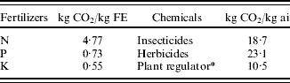
Two types of fertilizers (N and Starter Z, providing zinc (Zn)) are used in cotton farming systems in the Darling Downs region (Salmond Reference Salmond2002). Given that N-fertilizer is given in terms of N-amounts, there is no need for further recalculation for the estimation of N in this study. However, in the case of Starter Z, the proportion of N, P, K and Zn were estimated using their chemical formula and their molecular and atomic weights. For example, 100 kg of Starter Z contains 10·5 kg N, 19·2 kg P, 2·2 kg K and 2·5 kg Zn. As suggested by O'Halloran et al. (Reference O'Halloran, Fisher and Rab2008), each chemical was multiplied by a conversion factor (0·5 for herbicides and 0·25 for insecticides and plant growth regulator) to obtain the approximate active ingredients in the mix. CO2e emission factors for the production, packaging, storage and transportation of each kg of fertilizer-element (FE; in fertilizer) and active ingredient (in chemicals) were adapted from Lal (Reference Lal2004; Table 1). As Lal (Reference Lal2004) presented emission factors in C equivalent, they were converted into CO2e by multiplying by 3·67 (molecular wt of CO2/atomic wt of C=44/12).
Carbon dioxide equivalents (CO2e; kg CO2/kg FE or kg CO2/kg active ingredient chemicals (ai)) for production, packaging, storage and transportation of agrichemicals. Adapted from Lal (Reference Lal2004)

* Calculated using O'Halloran et al. (Reference O'Halloran, Fisher and Rab2008, p. 15).
Lal (Reference Lal2004) does not provide emission factors for plant growth regulator, and this was recalculated from information given in O'Halloran et al. (Reference O'Halloran, Fisher and Rab2008) .
Emissions of N2O from soils due to N-fertilizer application
N2O is responsible for 0·06 of observed global warming (Dalal et al. Reference Dalal, Wang, Robertson, Parton, Myer and Raison2003) and 0·063 of Australia's GHG emissions; however, this has rapidly increased from 0·043 in 1990 (Mitchell & Skjemstad Reference Mitchell and Skjemstad2004). Around 0·80 of N2O is produced by the agricultural sector, of which 0·73 is emitted from agricultural soils (Dalal et al. Reference Dalal, Wang, Robertson, Parton, Myer and Raison2003). Most of the N2O emissions come from N fertilizer usage and soil disturbances. Lack of oxygen or limited oxygen supply in the soil, or high oxygen demand due to more carbon food in the soil, causes micro-organisms to utilize nitrite (NO2−) and nitrate (NO3−) instead of oxygen. As a result of this de-nitrification process, the applied N-fertilizer is released as N2O into the atmosphere (Dalal et al. Reference Dalal, Wang, Robertson, Parton, Myer and Raison2003).
The IPCC set a default emission factor of 0·0125 (kg NO2-N emissions/kg of applied N). However, research has shown large variations from the IPCC default emission factor. In Australia, the CRC for Greenhouse Accounting has established a set of emission factors suitable for Australian agricultural systems (DCC 2005 cited in O'Halloran et al. Reference O'Halloran, Fisher and Rab2008). The values used in the present study were 0·005 (0·5 kg N2O-N/100 kg-N) for dryland cotton and 0·021 (2·1 kg N2O-N/100 kg-N) for irrigated cotton (DCC 2005 cited in O'Halloran et al. Reference O'Halloran, Fisher and Rab2008). After calculating the total amount of N2O-N, it was converted into N2O (by multiplying by 1·57; molecular wt of N2O/mole wt of N2) and then into CO2e.
GHG emissions due to the extraction, production and use of electricity for cotton irrigation
On average, cotton production in the Darling Downs region requires 4500 m3/year of water for cotton irrigation (Salmond Reference Salmond2002), as 0·92 of cotton production and 0·85 of total cotton area grown is surface irrigated. Thus, c. 4·6 GJ of energy is required to irrigate 1 ha of cotton each year through surface irrigation systems (Chen & Baillie Reference Chen and Baillie2007).
Emission factors for energy use also depend on the potentially mixed sources of energy, whether renewable or otherwise. For example, in Tasmania, most of the energy comes from hydroelectricity and thus emission factors are very low. The DCC regularly updates emission factors for each state of Australia, because the energy mix and thus emission factors may change over time. Scope 2 quantifies emissions due to the burning of fuels at power stations, whereas Scope 3 accounts for indirect emissions attributable to the extraction, production and transport of those fuels. Given the use of fossil fuels in cotton production, both Scope 2 and Scope 3 emission factors were considered in the present study. In 2005, emission factors (the sum of Scope 2 and Scope 3) for Queensland of 289 kg CO2e/GJ of energy were used (DCC 2009b; their Table 39).
Emissions due to the production of farm machinery in the cotton industry
Maraseni et al. (Reference Maraseni, Cockfield and Apan2007) investigated peanut–maize cropping in southeast Queensland, Australia and calculated the GHG emissions associated with the manufacture of each kg of farm machinery and accessories using eqn (1):

Data for peanut and maize cropping machinery operations were taken from Harden (Reference Harden2004), Wu & Perry (Reference Wu and Perry2004) and PCA (2008) and verified by relevant landholders and extension officers. Details about the working lifespan of farm machinery and accessories were obtained from Wu & Perry (Reference Wu and Perry2004) and the weight of machines and accessories were sourced from production companies John Deere and AMADAS. The fraction of time a particular machine was used for a particular operation was derived from crop management notes and independently verified by landholders and extension officers.
The present authors could not find any published information (number, types, sizes, power, etc.) about tractors and other accessories specifically used in the Australian cotton industry. Since machinery operations in the cotton industry are more closely aligned to peanut–maize cultivation, details from Maraseni et al. (Reference Maraseni, Cockfield and Apan2007) were used to inform the present study. Maraseni et al. (Reference Maraseni, Cockfield and Apan2007) concluded that GHG emissions due to farm machinery usage are directly related to fossil fuel consumption. In peanut–maize cultivation systems, GHG emissions due to farm machinery usage and accessories are 0·144 of emissions due to fossil fuels (Maraseni et al. Reference Maraseni, Cockfield and Apan2007). Negligible quantities of GHGs are emitted while transporting machinery and accessories and thus, as per Maraseni et al. (Reference Maraseni, Cockfield and Apan2007), they were not considered in the present study.
RESULTS
GHG emissions due to the production and combustion of fossil fuels used in cotton farming on the Darling Downs region
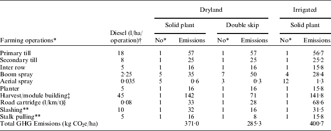
Table 2 presents a breakdown of GHG emissions from fossil fuel usage for a range of farming activities in the three common cotton farming systems in the Darling Downs region. Fossil fuels used in dryland solid-plant, dryland double-skip and irrigated farming, on aggregate, account for 371, 285 and 441 kg CO2e/ha of GHG emissions, respectively. Double-skip cotton farming systems require a larger number of boom sprays than the other two farming systems. However, because less fuel is used for harvesting operations, the double-skip farming system in total emits less GHG emissions than the other farming systems. Higher amounts of road transport-related GHGs emissions in irrigated cotton farming systems is attributed to higher production (1·81 t/ha (Salmond Reference Salmond2002)) compared to dryland solid-plant (0·86 t/ha) and dryland double-skip cotton farming systems (0·73 t/ha).
Emissions of GHG (kg CO2e/ha) due to the production and combustion of fossil fuels used in farming operations under three cotton farming systems in the Darling Downs region of southern Queensland, Australia

* Source: Salmond (Reference Salmond2002) .
† Source: Chen & Baillie (Reference Chen and Baillie2007) .
‡ Double skip farming system uses half the fuels of the other cotton farming systems.
§ For road transport estimation, a road distance of 150 km is used.
** Slashing and stalk pulling are post-harvest on-farm operations.
GHG emissions due to the production, packaging, storage and transportation of agrochemicals
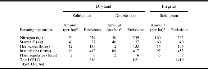
In total, the production, packing, storage and transportation of agrochemicals used in dryland solid-plant, dryland double-skip and irrigation cotton farming systems release 816, 821 and 1419 kg CO2e/ha emissions, respectively (Table 3). Irrigated cotton farming needs larger quantities of agrochemicals than other farming systems, but there is little difference in emissions among the three cotton farming systems from pesticides and plant regulators. Major differences are noted in the use of N and Starter Z fertilizers (Table 3). Irrigated cotton farming needs >1·5 times more Starter Z and >3 times more N-fertilizer than the other cotton farming systems. Due to these differences, GHG emissions from irrigated cotton farming are much higher than the other cotton farming systems.
Emissions of GHG (kg CO2e/ha) due to the use of agrochemicals for three cotton farming systems in the Darling Downs region of southern Queensland, Australia

* Source: Salmond (Reference Salmond2002) .
Emissions of N2O from soils due to N-fertilizer application
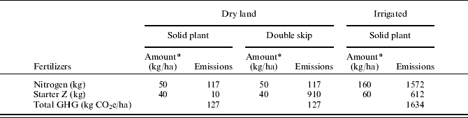
Solid-plant, double-skip and irrigated cotton farming systems in total emit around 127, 127 and 1634 kg CO2e GHGs per hectare, respectively into the atmosphere simply from de-nitrification of applied N fertilizer (Table 4). This emission is directly related to N-fertilizer amounts: the higher the N fertilizer use, the greater the emissions of N2O and thus the higher the CO2e. As Starter Z contains 0·105 N, its relative contribution to total emissions is quite low. Among the three cotton farming systems investigated, farmers use higher amounts of N fertilizer for irrigated cotton. Moreover, irrigated cotton has a higher N2O emission factor per kg of applied N-fertilizer than non-irrigated cotton. Due to these two factors, irrigated cotton emits >12 times more GHG emissions per hectare than from dryland cotton farming.
Emissions of N2O (kg CO2e/ha) from N-fertilizer application in soils under the three cotton farming systems in the Darling Downs region of southern Queensland, Australia

* Source: Salmond (Reference Salmond2002) .
GHG emissions due to the role of electricity in cotton irrigation
Dryland cotton farming does not use irrigation water and thus does not have electricity-related emissions. Irrigated cotton however uses 4500 m3 of irrigated water. Consequently, c. 1329 kg CO2e of GHG is emitted into the atmosphere simply through the use of electricity in cotton irrigation, thus representing the second largest source of GHG emissions (0·275 of all emissions) in irrigated cotton, after emissions from soils of N2O from N-fertilizer usage.
GHG emissions due to the production of farm machinery used in the cotton industry
The quantity of GHG emissions due to the use of farm machinery is directly related to fossil fuel-related emissions. Therefore, the irrigated cotton farming system has the highest machinery related emissions (58 kg CO2e/ha), followed by dryland solid-plant (53 kg CO2e/ha) and dryland double-skip (41 kg CO2e/ha) farming systems (Table 5).
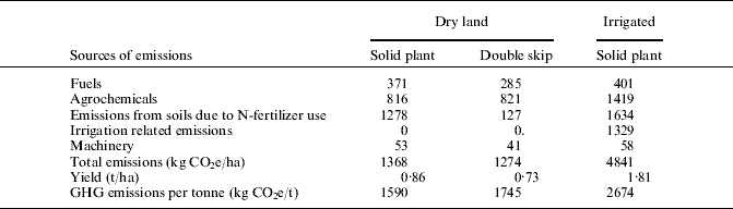
GHG emissions (kg CO2e/ha) due to various farming inputs from the three cotton farming systems in the Darling Downs region, southern Queensland, Australia

DISCUSSION
The aim of the present study was to quantify the ‘whole farm’ GHG emissions from three major cotton farming systems in the Darling Downs region of southern Queensland. In total, the highest quantities of GHGs are emitted from irrigated cotton farming (4841 kg CO2e/ha), followed by dryland solid-plant (1367 kg CO2e/ha) and dryland double-skip (1274 kg CO2e/ha; Table 5). Dryland cotton farming emissions are comparable to dryland peanut–maize cultivation in Kingaroy (a district immediately north of the Darling Downs), because peanuts are also a high input crop (Maraseni et al. Reference Maraseni, Cockfield and Apan2007). Higher amounts of GHG emissions from irrigated cotton farming are attributed to increased amounts of other farm inputs, especially the use of irrigation energy and greater use of N-fertilizers than the other cotton farming practices.
There is little difference in the quantities of GHG emissions per hectare between the two dryland cotton farming systems (Table 5). Dryland double-skip farming produces a lower yield (0·73 t/ha) than the other two cotton farming systems. GHG emissions per unit of production (t/ha) is highest in irrigated cotton farming systems, followed by dryland double-skip and dryland solid farming systems.
The analysis shows that 0·275 of total GHG emissions from irrigated cotton is related to electricity use for irrigation, 0·338 related to soils N2O emissions from N fertilizer use, 0·293 due to various agrochemicals, 0·083 due to farm fuel consumption and 0·0012 from farm machinery usage. These figures indicate that energy sources play a major role in GHG emissions; and that N management and the reduction of N2O from soils is crucial for reducing the carbon footprint of irrigated cotton.
There are several ways to minimize the N2O emissions from soils due to applied N-fertilizers including: (1) maintaining water-filled pore space at <0·4; (2) reducing soil compaction and thus increasing oxygen diffusion in soils; (3) reducing the readily available carbon supply, as this enhances microbial proliferation and N2O emissions; and (4) removing residual nitrate from the soil by growing cover crops (Dalal et al. Reference Dalal, Wang, Robertson, Parton, Myer and Raison2003). In addition, the opportunity provided by injecting biochar into soils is becoming a very popular means for reducing N2O emissions and fostering long-term soil carbon sequestration (Lehmann et al. Reference Lehmann, Gaunt and Rondon2006; Yanai et al. Reference Yanai, Toyota and Okazaki2007).
Queensland uses significant quantities of coal for electricity generation. Therefore, the emission factor for Queensland's electricity generation in 2005 is 289 kg CO2e/GJ. In comparison, Tasmania has been increasingly relying on hydropower for electricity generation, resulting in an emission factor of 12 kg CO2e/GJ (DCC 2009b; their Table 39). If Queensland cotton growers were able to use renewable energy then they would avoid irrigation related GHG emissions in the order of c. 1274 kg CO2e/ha. However, Tasmania is far from population centres and thus key produce markets, so the costs of crop transport could be appreciable.
Climate change may also impact cotton yield, yet there is a dearth of research in both Australia and elsewhere in this area. There is, however, research for other crop species that have highlighted climate change impacts on agricultural production. Research on rapeseed in Finland, which covers 0·93–0·99 of total oil crop cultivation area, showed that yields have fallen dramatically in the last 15 years, mainly due to enhanced crop sensitivity of the current rapeseed cultivars to elevated temperatures (Peltonen-Sainio et al. Reference Peltonen-Sainio, Jauhiainen and Hannukkala2007). A global study has highlighted that climate change will reduce agricultural production in all countries, except New Zealand, relative to the reference case (Gunasekera et al. Reference Gunasekera, Kim, Tulloh and Ford2007b, their Table 5). There is also some research showing that climate change impacts on agricultural production can be reduced by: (1) planting improved varieties (see Jaggard et al. (Reference Jaggard, Qi and Semenov2007), which make the case for sugar beet in UK); (2) following an adaptation plan (for instance wheat, beef and sheep production in Australia, see Gunasekera et al. Reference Gunasekera, Ford and Tulloh2007a; soybeans in northeast China, see Zheng et al. Reference Zheng, Chen and Han2009); and (3) following recommended best management practices (AGO 2006).
The research presented in the current paper is able to provide some insights into how much burden each type of cotton operation on the Darling Downs region will have to bear (1) if the CPRS becomes a reality; (2) if the CPRS covers all cotton growers without any benchmarking; (3) if there is no emissions intensive trade exposed (EITE) industry support for the cotton industry; and (4) if there is no fuel credit support as proposed in the CPRS (DCC 2008). If the carbon price is set at A$25/t CO2e, the irrigated cotton industry will bear the extra burden of A$121/ha (or A$66.8/t), for dryland solid-plant cotton industry A$34.20/ha (or A$39.7/t), and the dryland double-skip cotton industry will bear A$31.90/ha (or A$43.6/t). These figures highlight that differences in farming practices and farm inputs, make a significant difference in the resulting GHG emissions.
However, it is important to be cautious because these figures are averages or likely values; individual farms could have different emission factors and thus would attract different levels of financial burden. Furthermore, the present study has not considered some other sources of emissions such as those due to: (1) production and transportation of cotton packaging; (2) construction of buildings and building materials; (3) use of organic manures; (4) packing and overseas exportation; and (5) soil carbon. Therefore, the emissions figures and the extra burden calculations presented in the present study may be underestimated, and thus additional research on these details is needed.
In order to further reduce the potential burden of the CPRS, producers are likely to adapt no-tillage and stubble retention practices, which are the most popular ways to increase soil carbon sequestration and reducing fertilizer application rates as has been the case in North America and Europe, but these activities have not been very effective in Australia (Chan et al. Reference Chan, Cowie, Kelly, Singh and Slavich2009). Results from long-term trials in Wagga Wagga have shown that over a 20-year period, soil under traditional practices (stubble retention and traditional tillage) was losing carbon at a rate of 400 kg/ha/year compared to no-till and stubble retention (Heenan et al. Reference Heenan, Chan and Knight2004). Although, no-tillage and stubble retention were effective in reducing soil organic carbon losses, these activities did not increase soil organic carbon (Chan et al. Reference Chan, Cowie, Kelly, Singh and Slavich2009). In contrast with North America and Europe where severe winters decelerate the mineralization process, in Australia, relatively higher temperatures all year round favour the mineralization process (Chan et al. Reference Chan, Cowie, Kelly, Singh and Slavich2009). Moreover, no-tillage and stubble retention tend to increase N2O emission rates by increasing labile carbon into the soil, which in turn creates a favourable environment for N2O-producing micro-organisms (Dalal et al. Reference Dalal, Wang, Robertson, Parton, Myer and Raison2003). However, no-tillage and stubble retention promote weed growth; thus, controlling them requires greater amounts of herbicides, which have the highest global warming potential compared to other agrochemicals (Table 1). Therefore, common adaptation options such as no-till and stubble retention are less likely to reduce GHG emissions in Australia.
The current CPRS provisions are unlikely to cover the cotton industry. The CPRS is supposed to cover all sectors except agriculture from 2010, but the final decision of whether to include agriculture from 2015 will be made in 2013 (DCC 2008). Even if agriculture is covered, cotton farms may not come under the CPRS, as CPRS only covers entities with emissions >25 000 t CO2e/year. The present analysis shows that 1 ha of irrigated cotton farm (using the highest GHG emitting cotton farming system), on average, accounts for 4·84 t CO2e/ha/year. Thus, to be covered under the CPRS, the irrigated cotton farm would need to have at least 5165 ha of cotton, which is almost impossible as Australian cotton farms are typically 500–2000 ha (CRDC 2009) in size.
The present study, however, provides some valuable guidelines for the cotton industry. Firstly, based on this case study of the Darling Downs in southern Queensland, it provides hints for farmers and policy makers, where maximum GHG emissions are likely to come from and where attention should be focused on reducing GHG emissions. Secondly, it provides a basic database for developing a carbon calculator, as current cotton calculators in Australia do not consider GHG emissions due to agrochemical and machinery usage. Finally, it gives some insights to policy makers about where the cotton industry stands on GHG emissions and whether it is worth including this sector into the CPRS.
We would like to thank the Australian Centre for Sustainable Catchments, University of Southern Queensland, for research, logistical and other support. Our special thanks go to the Research and Higher Degrees, University of Southern Queensland, for financial assistance. Especially, we are greatly indebted to Greg Salmond, Queensland Primary Industries and Fisheries, for providing crop management notes and cotton data. Our special thanks go to Dr Guangnan Chen for information about fuel data and for his helpful discussion and suggestions.