





1. Introduction
We examine a variant of Darcy–Bénard convection, which is the porous medium analogue of the well-known Rayleigh–Bénard problem. The classical Darcy–Bénard configuration consists of a horizontal porous layer of uniform thickness with relatively hot lower and cold upper boundaries. Convection arises once the Darcy–Rayleigh number exceeds a critical value if the layer is supposed to be unbounded in both horizontal directions (Horton & Rogers Reference Horton and Rogers1945; Lapwood Reference Lapwood1948). This problem is one for which it is possible to conduct a weakly nonlinear analysis entirely analytically, The resulting equations demonstrate that two-dimensional rolls constitute the stable planform of convection, see for example Rees (Reference Rees2000) or Rees & Mojtabi (Reference Rees and Mojtabi2011). More complicated three-dimensional configurations, such as rectangles or hexagons, although mathematically acceptable solutions of the governing equations, prove to be unstable so are of limited physical relevance.
Post-critical planforms other than two-dimensional rolls are feasible with only modest changes to the basic configuration. For example, Jenkins & Proctor (Reference Jenkins and Proctor1984) discuss a case in which square cells are forced should the viscosity be strongly dependent on the temperature. On the other hand, both Riahi (Reference Riahi1983) and Rees & Mojtabi (Reference Rees and Mojtabi2011) have shown that square cells can be induced if there are conducting regions both above and below the porous layer. Wavy imperfections on the boundaries can also cause the preferred pattern to change. If these imperfections are of relatively long wavelength, rectangular cells are favoured (Rees & Riley Reference Rees and Riley1989a ) whilst much shorter wavelengths give rise to vortices with a wavy axis (Rees & Riley Reference Rees and Riley1989b ).
The original Darcy–Rayleigh formulation excludes various complicating factors including the effects of boundary and form-drag terms or allowing for an anisotropic permeability or temperature variations. Moreover, the heat transport equation also excludes these features as well as ignoring any temperature-dependent viscosity or local thermal non-equilibrium effects. Other changes are induced should the porous layer have imperfectly conducting boundaries (Riahi Reference Riahi1983) or possess some form of internal heating (Tveitereid Reference Tveitereid1977).
Several proposals have been forwarded as models to describe the nonlinear relationship between the pressure gradient and flow rate when inertial forces are accounted for. One popular choice is known as the Forchheimer effect, which supplements the standard Darcy’s law by a term which is quadratic in the fluid velocity. Another important property that needs to be recognised is that of viscous dissipation; we mention that Celli et al. (Reference Celli, de Alves and Barletta2016) incorporated this effect in a study of mixed convection in a Darcy–Bénard layer. When viscous dissipation is modelled by a velocity squared term, the strength of the dissipation is measured by the dimensionless Gebhart number. Simulations of the temperature within a sidewall heated porous cavity (Rees Reference Rees2007) or inside a cavity heated from below (Rees & Siddheshwar Reference Rees and Siddheshwar2025) have shown that, if the Gebhart number is allowed to become too large, this leads to the physically implausible result that regions inside the cavity achieve temperatures that exceed those of the heated boundaries. Indeed, Celli et al. (Reference Celli, de Alves and Barletta2016) have concluded that in most practical situations the Gebhart number must be small, although this may not necessarily be strictly true in some very large-scale geophysical contexts.
This observation motivated Rees & Magyari (Reference Rees and Magyari2017) to re-visit the Darcy–Bénard problem incorporating viscous dissipation terms. The small Gebhart number proved to be an ideal candidate for an expansion parameter on which to construct a weakly nonlinear theory. Rees & Magyari (Reference Rees and Magyari2017) examined the properties of hexagonal patterns formed from three separate roll solutions aligned at angles
 $60^\circ$
to each other. They demonstrated that hexagonal structures first appear at a Darcy–Rayleigh number which is somewhat lower than the critical value for the individual rolls themselves and the bifurcation to this weakly nonlinear state is transcritical. These hexagons constitute the preferred pattern near onset, but they eventually become unstable as the Darcy–Rayleigh number increases. By way of contrast, pure single-roll solutions are initially unstable but regain stability as this parameter grows. There is an intermediate regime within which both planforms are stable to small perturbations and within this parameter space an unstable mixed-mode pattern is theoretically possible. If form drag is present, then the onset of convection can become supercritical once form-drag effects are sufficiently strong.
Our motivation in this paper is to explore the competition between the rolls and hexagons in a porous layer when it is moved away from the horizontal and is inclined. It is known that, as the slope of the layer grows, so the critical Darcy–Rayleigh number increases for each roll; the size of this is a function of the orientation of the roll. We shall see that the introduction of the slope reduces the range of parameters over which stable hexagonal patterns are possible. Indeed, when the slope is sufficiently steep the only stable planform consists of longitudinal rolls. We determine this critical inclination and discuss how the well-known bifurcation structure for the horizontal layer is modified as the inclination increases.
We arrange the remainder of the work as follows. In § 2 we formulate the main equations and comment on the linear stability of individual rolls. These results enable us to deduce the coupled amplitude equations that govern structures when the layer is slightly inclined and this is discussed in § 3. Section 4 is devoted to an examination of the stability of longitudinal rolls while § 5 looks at the properties of three-dimensional convection in the geometry. We close with a few final remarks.
Schematic of the flow configuration. The layer occupies the region
 $0\leqslant \overline z\leqslant d$
, extends indefinitely in both the
 $\overline x$
and
 $\overline y$
directions and is inclined at an angle
 $\varGamma$
to the horizontal.

2. Formulation
Consider a layer of porous medium of width
 $d$
which is inclined at an angle
 $\varGamma$
to the horizontal. Co-ordinate axes
 $O\,\overline x\,\,\overline y\,\, \overline z$
are oriented so that the lower boundary is
 $\overline z=0$
, the
 $\overline x$
-axis is horizontal and the
 $\overline y$
-direction points up the slope; a sketch is shown in figure 1. The Darcy velocities in the three directions are denoted
 $\overline u$
,
 $\overline v$
and
 $\overline w$
and the pressure is
 $\overline p$
, while
 $T$
is the temperature of the saturated medium. In terms of these variables the equations that govern Boussinesq convection within the layer can be written
 \begin{align} &\frac {\partial \overline u}{\partial \overline x}+\frac {\partial \overline v}{\partial \overline y}+\frac {\partial \overline w}{\partial \overline z}=0,\quad \overline u = -\frac {K}{\mu }\frac {\partial \overline p}{\partial \overline x}, \\[-12pt]\nonumber \end{align}
 \begin{align} \overline v = -\frac {K}{\mu }\frac {\partial \overline p}{\partial \overline y}+\frac {\rho _fg\beta K}{\mu }&\left (T-T_{\textit{min}}\right )\sin \varGamma, \quad \overline w = -\frac {K}{\mu }\frac {\partial \overline p}{\partial \overline z}+\frac {\rho _fg\beta K}{\mu }\left (T-T_{\textit{min}}\right )\cos \varGamma \end{align}
and
 \begin{align} \big(\rho C_{\!p}\big)_m \frac {\partial T}{\partial \overline t} + \big(\rho C_{\!p}\big)_f\left [ \overline u\frac {\partial T}{\partial \overline x} +\overline v\frac {\partial T}{\partial \overline y}+\overline w\frac {\partial T}{\partial \overline z}\right ]=k\left [ \frac {\partial ^2 T}{\partial \overline x^2}+\frac {\partial ^2 T}{\partial \overline y^2}+\frac {\partial ^2 T}{\partial \overline z^2}+\right ] +\frac {\mu }{K}\big [ \overline u^2+ \overline v^2+ \overline w^2\big ]. \end{align}
Here,
 $K$
is the permeability,
 $g$
gravity,
 $\mu$
the fluid viscosity,
 $k$
the thermal conductivity of the saturated medium and
 $\beta$
the coefficient of cubical expansion. Moreover,
 $\rho$
is the density and
 $C_{\!p}$
the specific heat while the subscripts
 $m$
and
 $f$
are used to refer to the porous matrix and the saturating fluid, respectively. Finally,
 $T_{\textit{min}}$
and
 $T_{\textit{max}}$
denote the temperatures of the upper and lower boundaries, respectively.
Next, we write the problem in terms of suitable dimensionless variables. Lengths are expressed relative to the layer width
 $d$
, the velocities and time are scaled on
 $k/d (\rho C_0 )_f$
and
 $d^2k^{-1} (\rho C_0 )_m$
while the temperature is written as
 \begin{align} T=T_{\textit{min}}+(T_{\textit{max}}-T_{\textit{min}})\theta . \end{align}
Upon making these transformations we are led to the problem
 \begin{align} &\frac {\partial u}{\partial x}+\frac {\partial v}{\partial y}+\frac {\partial w}{\partial z}=0, \\[-12pt]\nonumber \end{align}
 \begin{align} u = -\frac {\partial p}{\partial x},\quad v = -\frac {\partial p}{\partial y}+&\textit{Ra}\,\theta \sin \varGamma, \quad w = -\frac {\partial p}{\partial z}+\textit{Ra}\,\theta \cos \varGamma \end{align}
and
 \begin{align} \frac {\partial \theta }{\partial t} + u\frac {\partial \theta }{\partial x} + v\frac {\partial \theta }{\partial y}+ w\frac {\partial \theta }{\partial z}= \frac {\partial ^2 \theta }{\partial x^2}+\frac {\partial ^2 \theta }{\partial y^2}+\frac {\partial ^2 \theta }{\partial z^2} +{\varepsilon }\left [ u^2+ v^2+ w^2\right ]. \end{align}
Our choice of variables throws up the viscous dissipation parameter
 $\varepsilon$
given by
 \begin{align} {\varepsilon }= \frac {\mu k}{(\rho C_{\!p})_f^2K(T_{\textit{max}}-T_{\textit{min}})}\equiv \frac {\textit{Ge}}{\textit{Ra}}, \end{align}
where
 \begin{align} \textit{Ge}= \frac {g\beta d}{C_{\!p}}\quad \mathrm{and}\quad \textit{Ra}= \frac {\rho g\beta (T_{\textit{max}}-T_{\textit{min}})Kd }{\mu (k/\rho C_{\!p})}, \end{align}
are the Gebhart and Darcy–Rayleigh numbers, respectively. For physically relatistic values
 $\varepsilon$
is very small, and this fact will be exploited to develop a weakly nonlinear description of the flow.
2.1. The basic flow
It is a straightforward exercise to deduce that the leading-order solution in
 $\varepsilon$
for the basic conduction flow is
 \begin{align} u=0,\quad v=v_B=\textit{Ra}\, \left (\frac 12-z\right )\sin \varGamma, \quad w=0, \\[-12pt]\nonumber \end{align}
 \begin{align} p=p_B=\frac 12\textit{Ra}\,z\left (2-z\right )\cos \varGamma +\frac 12\textit{Ra}\,y\sin \varGamma, \quad \theta =\theta _B=1-z. \end{align}
Equations for disturbances to the basic state are best derived by eliminating the fluid velocities
 $u,v$
and
 $w$
from the continuity and temperature balances ((2.3a
), (2.3e
)) using (2.3b
–
d
). If we write
 \begin{align} p=p_B+P,\quad \theta =\theta _B+\varTheta, \end{align}
then
 \begin{align}{\nabla} ^2P=\textit{Ra}\,\left \{ \varTheta _y \sin \varGamma +\varTheta _z\cos \varGamma \right \}\, \end{align}
and
 \begin{align} &{\nabla} ^2\varTheta +\textit{Ra}\,\varTheta -P_z =\frac 12{\varepsilon }^2\varTheta _\tau -\boldsymbol{\nabla }\!P\boldsymbol{\cdot }\boldsymbol{\nabla }\varTheta +\textit{Ra}\,\varTheta \left (\sin \gamma \varTheta _y+\cos \gamma \varTheta _z\right )\nonumber \\ &\qquad \qquad \qquad +\textit{Ra}\,\varTheta (1-\cos \gamma ) +\textit{Ra}\,\varTheta _y\left (\frac 12-z\right )\sin \gamma \nonumber \\ &\,-{\varepsilon }\left [ \left ( P_x\right )^2 +\left ( v_B -P_y+\textit{Ra}\,\varTheta \sin \varGamma \right )^2+ \left ( -P_z+\textit{Ra}\,\varTheta \cos \varGamma \right )^2\right ]\!. \end{align}
Modes close to the onset of instability evolve on the slow time scale
 \begin{equation} \tau =\frac 12{\varepsilon } ^2t, \end{equation}
which has been introduced in (2.8b ). The system needs to be solved subject to the homogeneous boundary conditions
 \begin{equation} P_z=\varTheta =0\quad \mathrm{on}\quad z=0,1. \end{equation}
2.2. Linear theory
Before we outline the linear stability characteristics of our basic flow, we need to set the inclination of the layer that will deliver the appropriate amplitude equations. Ideally, we need the effects of the viscous dissipation and of the slope to be of comparable sizes. We know from the analysis of Rees & Magyari (Reference Rees and Magyari2017) that the key nonlinear interactions arise at a size
 ${\mathcal O}({\varepsilon }^2)$
smaller than the amplitudes of the constituent rolls. On the other hand, the results derived by Rees & Bassom (Reference Rees and Bassom2000) for classical Darcy–Bénard convection suggests that for small slopes
 $\varGamma$
the change to the critical value of
 $\textit{Ra}$
is
 ${\mathcal O}(\varGamma ^2)$
. To ensure
 $\varGamma ^2\sim {\varepsilon }^2$
we put
 \begin{equation} \varGamma =\varepsilon \gamma \quad \mathrm{with}\quad \gamma ={\mathcal O}(1) \end{equation}
and study a roll at orientation
 $\phi$
. We seek a solution of system (2.8) with
 \begin{align} (\varTheta, P)=\varDelta \big ( \varTheta _{0L}(z)+{\varepsilon }\varTheta _{1L}(z)+{\varepsilon }^2\varTheta _{2L}(z)+\ldots, P_{0L}(z)+{\varepsilon } P_{1L}(z)+{\varepsilon }^2 P_{2L}(z)+\ldots \big)E+\mathrm{c.c.}, \end{align}
where
 \begin{equation} E\equiv \exp \left \{ ia(x\cos \phi +y\sin \phi )\right \} \!; \end{equation}
here, we are supposing that
 $0\lt \varDelta \ll 1$
and note that c.c. denotes the complex conjugate. If we write
 \begin{align} \textit{Ra}\,=\textit{Ra}_0\,+{\varepsilon }\,\textit{Ra}_1+{\varepsilon }^2 \textit{Ra}_2+\ldots, \end{align}
then the substitution of (2.12) into the linearised reduction of system (2.8) leads to a hierarchy of equations for the eigenfunctions. The zeroth-order equations admit a non-trivial solution if
 \begin{align} \textit{Ra}_0=\frac {(a^2+\pi ^2)^2}{a^2}; \end{align}
this is minimised when
 $a=\pi$
and then
 \begin{equation} \textit{Ra}_0=4\pi ^2,\quad \varTheta _{0L}=Q(\tau )\sin \pi z\quad \mathrm{and} \quad P_{0L}=-2\pi Q(\tau )\cos \pi z. \end{equation}
The next order equations for
 $P_{1L}$
and
 $\varTheta _{1L}$
only have a solution if
 $\textit{Ra}_{1}=0$
, whereupon we have
 \begin{align} P_{1L}=\frac 12i\pi \gamma Q(\tau )\sin \phi \big[ 2 \big(\pi ^2(z-1)-1\big)\sin \pi z+\pi \left (2z-1\right )\cos \pi z\big ], \\[-12pt]\nonumber \end{align}
 \begin{align} \varTheta _{1L}=\frac 14i\pi \gamma Q(\tau )\sin \phi \left [ \left (1-2z\right )\sin \pi z+2\pi z(z-1)\cos \pi z\right ]\!. \end{align}
Finally, the second-order equations for
 $\varTheta _{2L}$
and
 $P_{2L}$
are compatible only if
 \begin{equation} \frac {{\rm d}Q}{{\rm d}\tau }=\big\{ \textit{Ra}_{2}-(2+3\sin ^2\phi )\gamma ^2\pi ^2 \big \}Q, \end{equation}
which shows that the onset of instability occurs when
 \begin{equation} \textit{Ra}_{\mathrm{c}}(\phi )=4\pi ^2 + \varepsilon ^2\gamma ^2\pi ^2 \big[ 2 + 3\sin ^2\phi \big] + o(\varepsilon ^2). \end{equation}
3. The weakly nonlinear evolution equations
The study of Rees & Magyari (Reference Rees and Magyari2017) was concerned with the effect of viscous dissipation on the preferred hexagonal planform of convection within a horizontal layer. Given the results of the linear theory outlined above, we now can explore the fate of this structure as the layer is increasingly inclined. Guided by the prediction (2.19), we suppose that
 \begin{equation} \textit{Ra}= 4\pi ^2 + \varepsilon ^2 R_2 + {\cdots}, \end{equation}
and look for solutions of the form
 \begin{equation} \left (\varTheta, P\right )={\varepsilon }(\varTheta _1,P_1)+{\varepsilon }^2(\varTheta _2,P_2)+{\varepsilon }^3(\varTheta _3,P_3)+\ldots . \end{equation}
Our hexagonal planform is constructed from three rolls that are set at mutual orientation angles of
 $60^\circ$
. Accordingly, the
 $\mathcal{O}(\varepsilon )$
temperature perturbation takes the form
 \begin{align} \varTheta _1 = \frac {1}{2\pi ^2} \bigl [ \textit{AE}_1 + \textit{BE}_2+\textit{CE}_3 +\hbox{c.c.} \bigr ] \sin \pi z, \end{align}
where the three complex roll amplitudes
 $A$
,
 $B$
and
 $C$
are functions of the slow time scale
 $\tau$
and the functions
 $E_1, E_2$
and
 $E_3$
are of the form (2.13) with
 $a=\pi$
and angles
 $\phi =0$
,
 $60^\circ$
and
 $-60^\circ$
, respectively. The corresponding pressure solution is
 \begin{align} P_1 = -\frac {1}{\pi } \bigl [ \textit{AE}_1 + \textit{BE}_2 + \textit{CE}_3 +\hbox{c.c.} \bigr ] \sin \pi z; \end{align}
the choice of prefactors has been made in order to simplify the coefficients in the final amplitude equations as far as possible.
Given the solution (3.3) the solution at the next order becomes
 \begin{align} \varTheta _2 =& \frac {1}{2\pi ^2} \big [ A\overline A +B\overline B+C\overline C\big ] -\frac {7}{148\pi ^3}\big [ AB\,E_1E_2 + AC\, E_1E_3 +BC\, E_2E_3 +\mathrm{c.c.}\big ] \sin 2\pi z \nonumber \\ &\qquad \qquad \qquad -\frac {5}{28\pi ^3}\big [A\overline B\,E_1E_2^{-1} + A\overline C\, E_1E_3^{-1} +B\overline C \,E_2\,{E_3}^{-1} +\mathrm{c.c.}\big ]\sin 2\pi z \nonumber \\ &+\frac {3}{32\pi }\gamma \big[ (1-2z)\sin \pi z+2\pi z(z-1)\cos \pi z\big ] \big \{i (\textit{CE}_3-\textit{BE}_2)+\mathrm{c.c.}\big \} \end{align}
and
 \begin{align} P_2 =& -\frac {1}{4\pi ^3} \big [ A\overline A +B\overline B+C\overline C\big ] +\frac {2}{37\pi ^2}\big [ AB\,E_1E_2 + AC\, E_1E_3 +BC\, E_2E_3 +\mathrm{c.c.}\big] \cos 2\pi z \nonumber \\ &\qquad +\frac {2}{7\pi ^2}\big [A\overline B\,E_1E_2^{-1} + A\overline C\, E_1E_3^{-1} +B\overline C \,E_2\,{E_3}^{-1} +\mathrm{c.c.}\big ]\cos 2\pi z \nonumber \\ &+\frac {3}{16\pi }\gamma \big [ 2 (\pi ^2(z-1)-1)\sin \pi z+\pi (2z-1)\cos \pi z\big ] \big \{i (\textit{CE}_3-\textit{BE}_2)+\mathrm{c.c.}\big \}. \end{align}
We point out that the these fields are non-resonant owing to the symmetries in the
 $z$
-dependence. This means that the important amplitude equations will be deferred to the next order solution in
 ${\mathcal O}({\varepsilon }^3)$
. The application of suitable solvability conditions at this point leads to a system of Landau equations which may be cast as
 \begin{align} &A_\tau = \,\, \textit{SA} \,\,\,\, - A^2\overline {A} - \varOmega A( B\overline {B} + C\overline {C}) + \alpha BC, \\[-12pt]\nonumber \end{align}
 \begin{align} B_\tau =& \,\, \left(S - \frac {9}{4}\pi ^2\gamma ^2 \right)B - B^2\overline {B} - \varOmega B( A\overline {A} + C\overline {C}) + \alpha A\overline {C}, \\[-12pt]\nonumber \end{align}
 \begin{align} C_\tau =& \,\, \left(S - \frac {9}{4}\pi ^2\gamma ^2 \right)C - C^2\overline {C} - \varOmega C( A\overline {A} + B\overline {B}) + \alpha A\overline {B}, \end{align}
where a slight simplification has been achieved by setting
 $R_2 = S + 2\pi ^2\gamma ^2$
. The value of the coupling coefficient
 $\varOmega$
depends on the relative orientations of the two rolls; if this angle is
 $\phi$
then it can be shown that
 \begin{align} \varOmega (\phi )=\frac {70+28\cos ^2\phi -2\cos ^4\phi }{49-2\cos ^2\phi +\cos ^4\phi } \end{align}
and for our configuration
 $\varOmega =410/259$
. The quadratic terms arise directly from the presence of viscous dissipation and are multiplied by the coefficient
 $\alpha \equiv 16\pi$
. Finally, we note that the spatial interaction of a
 $B$
-roll and a
 $C$
-roll generates an
 $A$
-roll.
Relative to a background zero state, it is immediately clear that
 $S=0$
is the point of neutral stability for the longitudinal rolls (
 $A$
) while it is
 $S=( 9/4)\pi ^2\gamma ^2$
for the oblique rolls (
 $B$
,
 $C$
).
4. The stability of longitudinal rolls
The basic state corresponding to a longitudinal roll is simply
 \begin{equation} A=S^{1/2}, \quad B=C=0, \end{equation}
which clearly only exists if
 $S\gt 0$
. Without loss of generality we may suppose that this basic state is real. We perturb this solution using
 \begin{equation} A=S^{1/2}+{\delta A}\, e^{\lambda \tau }, \quad B={\delta B}\, e^{\lambda \tau }, \quad C={\delta C}\, e^{\lambda \tau }, \end{equation}
in which
 $\delta A$
,
 $\delta B$
and
 $\delta C$
are all small while
 $\lambda$
is the exponential growth rate. The substitution of the forms (4.2) into system (3.5) followed by linearisation yields
 \begin{align} &\qquad \lambda \,{\delta A} = -S\,{\delta A} - S\,\overline {{\delta A}}, \\[-12pt]\nonumber \end{align}
 \begin{align} \lambda \,{\delta B} =& \left (S-\frac 94\pi ^2\gamma ^2\right ){\delta B} - \varOmega S\, {\delta B} + \alpha S^{1/2}\, \overline {{\delta C}}, \\[-12pt]\nonumber \end{align}
 \begin{align} \lambda \,{\delta C} =& \left (S-\frac 94\pi ^2\gamma ^2\right ){\delta C} - \varOmega S\, {\delta C} + \alpha S^{1/2}\,\overline {{\delta B}}. \\[10pt] \nonumber \end{align}
Clearly, the equation for the longitudinal roll is decoupled form the others. If we solve for
 $\delta A$
it is straightforward to show that
 $\lambda$
takes two possible values: either
 $\lambda =-S$
with
 $\delta A$
purely real or
 $\lambda =0$
and
 $\delta A$
is then imaginary. Therefore, we conclude that real perturbations decay exponentially, while imaginary perturbations are neutrally stable; this latter case simply corresponds to phase shifts in the
 $A$
-roll.


We next turn to the equations for
 $\delta B$
and
 $\overline {{\delta C}}$
within system (4.3). If we take the complex conjugate of (4.3c
) we deduce that
 \begin{equation} \lambda \begin{pmatrix} {\delta B} \\ \\ \overline {{\delta C}} \end{pmatrix} = \begin{pmatrix} (1-\varOmega )S-\frac 94\pi ^2\gamma ^2 & \alpha S^{1/2} \\ &\\ \alpha S^{1/2} & (1-\varOmega )S-\frac 94\pi ^2\gamma ^2 \\ \end{pmatrix} \begin{pmatrix} {\delta B} \\ \\ \overline {{\delta C}} \end{pmatrix}\!; \end{equation}
the symmetry of the matrix implies that
 $\lambda$
is real and elementary algebra yields
 \begin{equation} \lambda = (1-\varOmega )S - \frac 94\pi ^2\gamma ^2 \pm \alpha S^{1/2}. \end{equation}
The smaller of these two values is always negative, which implies stability, and this decaying mode has
 ${\delta B}=-\overline {{\delta C}}$
. The larger value of
 $\lambda$
vanishes when
 $S=S_{\pm }$
where
 \begin{equation} S_{\pm }^{1/2} = \frac { \alpha \pm \left [\alpha ^2 - 9\pi ^2(\varOmega -1)\gamma ^2\right ]^{1/2} }{2(\varOmega -1)}, \end{equation}
with a corresponding mode shape
 ${\delta B}=\overline {{\delta C}}$
.
Given a particular value
 $\gamma$
, we conclude that, if
 $S_-\leqslant S\leqslant S_+$
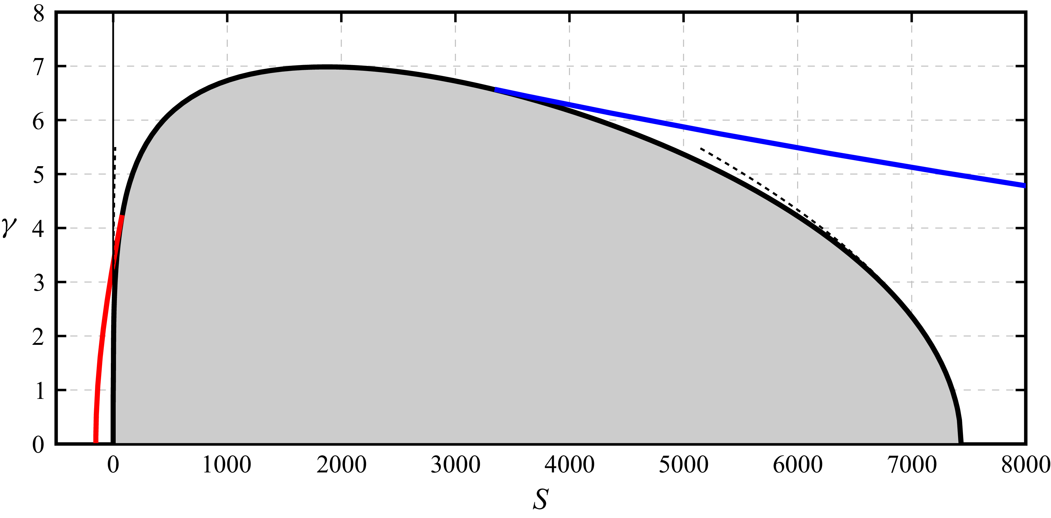
, then the longitudinal rolls are unstable. The unstable region in
 $(S,\gamma )$
parameter space is shaded grey in figure 2. We remark that as
 $\gamma$
increases so the values
 $S_-$
and
 $S_+$
coincide when
 \begin{equation} \gamma =\frac {\alpha }{3\pi \sqrt {\varOmega -1}} = 6.984899, \end{equation}
while the corresponding value of
 $S$
is
 \begin{equation} S=\frac {\alpha ^2}{4(\varOmega -1)^2} = 1858.34. \end{equation}
We may also use expression (4.6) to deduce polynomial approximations for the range of instability for rolls. As long as
 $\gamma$
is not too large, we conclude that
 \begin{equation} \frac {81\pi ^2\gamma ^4}{16\alpha ^2} \lesssim S \lesssim \frac {\alpha ^2}{(\varOmega -1)^2} - \frac {9\pi ^2\gamma ^2}{2(\varOmega -1)}; \end{equation}
these bounds are superimposed as dashed lines on figure 2. We comment that the lower limit is virtually indistinguishable from the vertical axis while the upper bound is very accurate even for values of
 $\gamma$
as large as
 $5$
. (We point out that the upper bound for the instability of rolls does not reduce to the result quoted in Rees & Magyari Reference Rees and Magyari2017 when
 $\gamma =0$
; this is due to a typographical error in that paper.)
5. Three-dimensional convection
5.1. A horizontal layer
When the layer is horizontal the natural convection pattern that is seen close to onset has a hexagonal planform; this is a direct consequence of the fact that
 $A$
,
 $B$
and
 $C$
have equal magnitudes. It follows that the solution is given by
 \begin{equation} A=B=C = \frac {\alpha \pm \Bigl [ \alpha ^2+4S(1+2\varOmega ) \Bigr ]^{1/2} }{2(1+2\varOmega )}, \end{equation}
which exists for
 $S\gt -\alpha ^2/4(1+2\varOmega )$
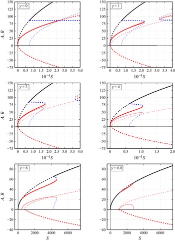
. This solution is shown in the first panel of figure 3 in the vicinity of
 $S=0$
at which point there is a transcritical bifurcation. It is well known that the upper solution branch is stable while the lower one is unstable. This is indicated in figure 3 by using a continuous (dashed) line for stable (unstable) solutions; this convention is maintained for the subsequent results.
As well as the solution with three rolls of equal size there is a second possibility in which the longitudinal roll is of a different strength to the oblique modes. In particular
 \begin{equation} A=A^*\equiv \frac {\alpha }{\varOmega -1}, \quad B=C=\left [ \frac { S - (A^*)^2 }{\varOmega +1} \right ]^{1/2}; \end{equation}
a solution which exists when
 $S\gt (A^*)^2$
which is precisely the range over which the longitudinal roll is stable; see result (4.9) with
 $\gamma =0$
. This mixed-mode solution (which is shown in blue in the first panel of figure 4) arises as a bifurcation from the longitudinal roll. As
 $S$
grows so the mixed mode persists until
 $S=(\varOmega +2)\alpha ^2/(\varOmega -1)^2$
at which point it is identical to the hexagonal solution. Simultaneous with this the hexagonal solution loses its stability as
 $S$
increases further; these features are summarised in figure 4.
5.2. An inclined layer
In order to study the properties of convection within an inclined layer we solve the steady form of system (3.5) as a function of
 $S$
for various chosen values of
 $\gamma$
. Before we describe the results, we first make a helpful observation. Within the equations (3.5), if the amplitudes
 $A$
,
 $B$
and
 $C$
are replaced by
 $Ae^{ia}$
,
 $Be^{ib}$
and
 $Ce^{ic}$
, respectively, with
 $a=b+c$
, then the system is unchanged. Therefore we can take
 $A$
 $B$
and
 $C$
to be real without any loss of generality. To simplify matters further, we remark that the most unstable disturbance of the longitudinal roll occurs when
 ${\delta B}={\delta C}$
so we solve equations (3.5) with
 $B=C$
and then solve for
 $A$
and
 $B$
. The resulting steady-state equations become
 \begin{align} &\qquad \qquad \quad \textit{SA} - A^3 - 2\varOmega A B^2 + \alpha B^2 = 0, \\[-12pt]\nonumber \end{align}
 \begin{align} & \left(S-\frac 94\pi ^2\gamma ^2\right)B - (1+\varOmega )B^3 - \varOmega B A^2+ \alpha AB=0. \end{align}
Solutions of these equations were obtained using an elementary Newton–Raphson scheme. Given a fixed value of
 $\gamma$
the variation of
 $A$
and
 $B$
with
 $S$
was explored. The results of the computations are displayed in figures 3 and 4. In these figures the black curves correspond to longitudinal rolls with
 $B=C=0$
while the red and blue curves correspond to fully three-dimensional patterns; the former are referred to as being pseudo-hexagonal whilst the latter are deemed mixed-mode patterns. This designation was adopted because the red curves evolve from the hexagonal form (5.1) as
 $\gamma$
changes while the genesis of the blue curves can be traced to the mixed-mode solution (5.2).
Solution curves at four values of
 $\gamma$
and with
 $S\leqslant 10^3$
. Black lines correspond to longitudinal rolls; red lines denote pseudo-hexagonal patterns. Linearly stable (unstable) solutions are indicated by continuous (dashed) lines. Thick lines show the value of
 $A$
while the thin ones correspond to the size of
 $B$
.

Solution curves for selected values of
 $\gamma$
but extended to larger values of
 $S$
. Colours and line conventions are as in figure 3 except that here the additional blue lines denote mixed modes.

As
 $\gamma$
increases from zero, figure 3 shows that the continuous curve representing the lower branch of the hexagonal solution curve breaks in two. The transcritical bifurcation at the origin is replaced by a supercritical bifurcation at a positive value of
 $S$
and a subcritical bifurcation from the longitudinal solution curve at a smaller (but still positive) value of
 $S$
. We may easily determine the form of the supercritical bifurcation. The critical value of
 $S$
is
 \begin{equation} S=S_c\equiv \frac 94\pi ^2\gamma ^2, \end{equation}
and it follows that
 $A$
varies linearly and that
 $B$
assumes the familiar square root variation with
 $S-S_c$
as
 $S$
grows. The curves shown in figure 3 clearly illustrate these properties.
Figures 3 and 4 together show that the bifurcation from the longitudinal roll to a three-dimensional pattern is often supercritical but sometimes becomes subcritical. We can investigate this phenomenon using a standard weakly nonlinear theory. If the bifurcation from the roll occurs at
 $S=S_0$
then nearby we suppose that
 \begin{equation} S=S_0 + \delta ^2 S_2 + {\cdots}, \quad A=\sqrt {S_0} + \delta ^2 A_2 + {\cdots}, \quad B= \delta B_1 + \delta ^3 B_3 + {\cdots}, \end{equation}
where
 $\delta \ll 1$
. The
 ${\mathcal O}(\delta )$
terms in the steady-state (5.3b
) yield
 \begin{align} (\varOmega -1)S_0 - \alpha \sqrt {S_0} + \frac 94\pi ^2\gamma ^2=0\quad \Longrightarrow \quad \sqrt {S_0}=\widehat {S}_\pm = \frac { \alpha \pm \sqrt {\alpha ^2 - 9(\varOmega -1)\pi ^2\gamma ^2}}{2(\varOmega -1)}, \end{align}
which confirms the stability analysis for rolls given by (4.5) with the plus sign. The
 ${\mathcal O}(\delta ^2)$
terms in (5.3a
) show that
 \begin{equation} A_2 = \frac { \sqrt {S_0} S_2 + (\alpha - 2\varOmega \sqrt {S_0}) B_1^2 }{2S_0}, \end{equation}
whence the second steady-state (5.3b ) yields
 \begin{equation} \left [ \frac { \alpha - 2(\varOmega -1)\sqrt {S_0} }{2\sqrt {S_0}} \right ] S_2 + \left [ \frac { (\alpha -2\varOmega \sqrt {S_0})^2 }{2S_0} - (1+\varOmega ) \right ] B_1^2 =0. \end{equation}
Elementary algebra shows that
 $S_2\gt 0$
when
 $ \sqrt {S_0}=\widehat {S}_-$
for all values
 $\gamma$
; hence this is always a supercritical bifurcation. For
 $ \sqrt {S_0}=\widehat {S}_+$
this result continues to hold for
 $\gamma \lt \gamma _c$
where
 \begin{equation} \frac {9}{256}\gamma _c^2\equiv \frac {2\varOmega +\sqrt {2(1+\varOmega )}}{1+2\varOmega }\quad \Longrightarrow \gamma _c\approx 6.09, \end{equation}
but at larger values the sign of
 $S_2$
switches so
 $S_2\lt 0$
. This implies that once
 $\gamma$
exceeds
 $\gamma _c$
the nature of the bifurcation to the hexagon from the roll becomes subcritical; a result that is consistent with the results in the final panel of figure 4.
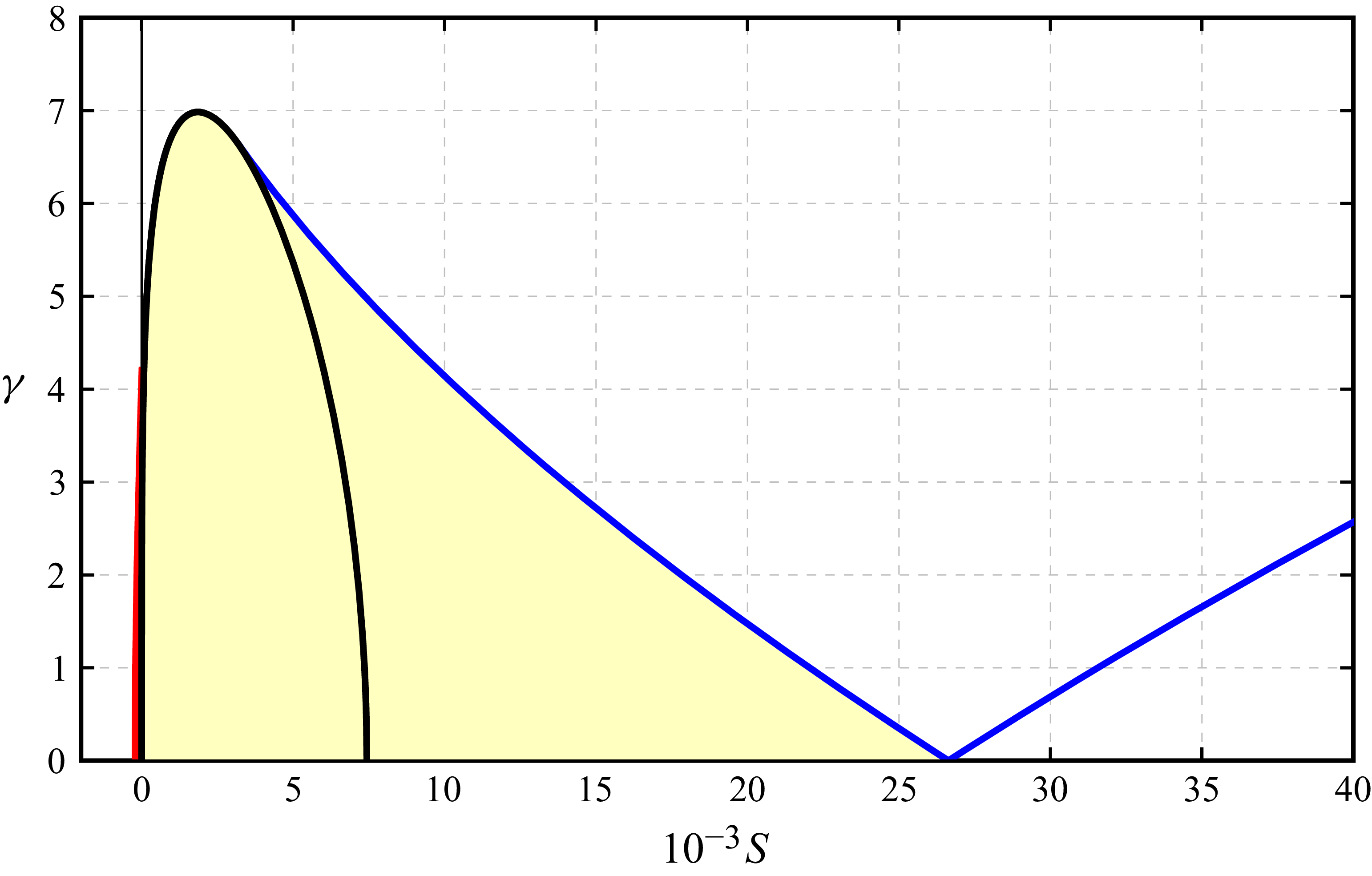
The light yellow region shows where pseudo-hexagonal cells exist and are stable. The red curve shows the smallest value of
 $S$
for which pseudo-hexagons are possible. The blue curves depict the two fold bifurcations which connect the pseudo-hexagons and the mixed-mode curves.

5.3. The fold bifurcation
The computations summarised in figure 4 show that the hexagonal and mixed-mode solutions are connected via a pair of fold bifurcations. As
 $\gamma$
increases from 0 so these folds separate; their locations as functions of
 $\gamma$
are shown in figure 5. Here, we illustrate the region of parameter space in which the hexagonal cells are stable while the two blue lines denote the positions of the folds as functions of
 $\gamma$
.
We can derive some elementary equations that help in the analysis of the folds. We begin by eliminating the mode amplitude
 $B$
between equations ((5.3a
), (5.3b
)) to leave
 \begin{equation} (1+\varOmega )A(S - A^2) +(\alpha - 2\varOmega A)\left (S-\frac 94\pi ^2\gamma ^2+\alpha A-\varOmega A^2\right ) = 0. \end{equation}
We might normally think of this as an equation for
 $A$
in terms of the other parameters, but for the purpose of locating the folds it is much more convenient to regard (5.10) as a recipe for
 $S=S(A)$
. At a fold there is a turning point in
 $S$
so if we differentiate (5.10) with respect to
 $A$
it follows that, at the fold,
 \begin{equation} (1-\varOmega )S +3(\varOmega -1)(2\varOmega +1)A^2-6\alpha \varOmega A+\alpha ^2+\frac 92\varOmega \pi ^2 = 0. \end{equation}
We can combine results ((5.10), (5.11)) to deduce that
 \begin{align} 2(\varOmega -1)(2\varOmega +1)A^3-3(3\varOmega +1)\alpha A^2 +\frac {6\varOmega }{\varOmega -1}\alpha ^2A-\frac {\alpha ^3}{\varOmega -1} -\frac 94\pi ^2\alpha \left (\frac {\varOmega -1}{\varOmega +1}\right )\gamma ^2 = 0 \end{align}
and
 \begin{align} S=3(2\varOmega +1)A^2- \frac {6\varOmega }{\varOmega -1}\alpha A+\frac {\alpha ^2}{\varOmega -1}+\frac 92\pi ^2\left (\frac {\varOmega }{\varOmega -1}\right )\gamma ^2. \end{align}
It is worth pointing out that no approximations have been involved in the derivation of these equations for the folds. Although we cannot solve them completely, it is possible to develop series solutions for small
 $\gamma$
 \begin{align} &\qquad A\approx \frac {\alpha }{\varOmega -1} \pm \frac {\pi \sqrt 3}{\sqrt {4(\varOmega -1)}}\gamma -\frac {\pi ^2(2\varOmega +1)}{4(\varOmega +1)}\frac {\gamma ^2}{\alpha }+\ldots, \\[-12pt]\nonumber \end{align}
 \begin{align} S\approx \alpha ^2 &\left \{ \frac {\varOmega +2}{(\varOmega -1)^2} \pm \frac {3\sqrt 3 \pi (\varOmega +1)}{(\varOmega -1)^{3/2}}\frac {\gamma }{\alpha }+\frac {3\pi ^2(8\varOmega +1)}{4(\varOmega -1)}\frac {\gamma ^2}{\alpha ^2}+\ldots \right \}\!. \end{align}
We recall that our calculations have been conducted with
 $\alpha =16\pi$
and then these series solutions are accurate for all the values of
 $\gamma$
shown in figure 5. Finally, we mention that the solution for the fold at the smaller value of
 $S$
remains valid until we reach the point when
 $B=0$
(or
 $A=\sqrt {S}$
). Equation (5.10) shows that this occurs when
 $S=\widehat {S}_+$
as defined in (5.6); at greater values of
 $\gamma$
the pseudo-hexagon bifurcates from the roll solution.
Last, we mention in passing that the solutions (5.13a
) are two solutions of the cubic equation (5.12a
). It is straightforward to show that the third solution corresponds to a value
 $S\lt 0$
which is of no interest here.
6. Closing remarks
In this study we have examined the combined effects of viscous dissipation and layer inclination on classical Darcy–Bénard convection. We have shown that the introduction of the small slope of the layer can play an important part in controlling the form of the feasible convection patterns. When the layer is horizontal, hexagonal patterns are possible with all three pairs of constituent rolls of equal amplitudes but as the layer is gradually inclined this is no longer a realisable scenario. Rather, a mixed-mode structure is established whose nature has been described herein. In particular, it has been demonstrated that, as the slope of the layer grows, so the remnant of the hexagonal structure gradually weakens. Indeed, there is a point at which the hexagon is destroyed completely and what remains is just a simple two-dimensional roll. An alternative interpretation of this result is that were the slope of the layer
 $\varGamma$
be fixed, a reduction in the size of
 $\varepsilon$
would cause the hexagonal planform to vanish at some stage.
There are various generalisations and modifications that could be envisaged. One possibility would be to examine the situation that arises should one of the rolls be transverse. It is quite likely that while there may be islands of stability when attention is confined to just the three rolls, it is probable that this would prove to be a subdominant pattern. Mention should also be made of the problem which arises when the overall pattern consists of six orientations and two hexagons: one could then probe the stability of the second hexagon with respect to rolls of the first. Finally, there is the possibility of hexagonal structures in which no roll is either longitudinal or transverse; this will lead to the situation of three rolls with different amplitudes and would represent a somewhat formidable analytical exercise.
Declaration of interests
The authors report no conflict of interest.
The referees are thanked for their helpful comments which have led to a much improved paper.

 0⩽z¯⩽d
 x¯
 y¯
 Γ
 (S,γ)
 γ

 γ
 S⩽103
 A
 B
 γ
 S
 S

 Open access

