1. Introduction
For some considerable time, one of the most important areas of research in jet acoustics has been the development and application of improved techniques for accurate measurement of whole-field spatio-temporal turbulence correlations. The fourth-order two-point two-time correlation of the fluctuating Reynolds stress (
 $r_{ij,kl}$
– to be defined below) has long been recognised as the fundamental statistical property of jet turbulence, acting as the acoustic source in broadband jet mixing noise (Lighthill Reference Lighthill1952, Reference Lighthill1954). Proudman (Reference Proudman1952), for example, used the Lighthill theory to show that the acoustic intensity at any point in the far field was related to a volume integral of the fourth-order time derivative of the two-point two-time correlation of the fluctuating Reynolds stress tensor. Assumptions about this property are an inherent part of all jet noise models (Morris & Farassat Reference Morris and Farassat2002). Direct measurements of this correlation to judge the accuracy of the various approximations proposed for its modelling are therefore crucial for progress towards improved jet noise simulation.
Historically, data on spatio-temporal correlations in jets were first obtained using hot-wire anemometry (HWA). This has excellent temporal response – up to
 ${\sim}50~\text{kHz}$
– but it is a single-point technique and spatial resolution relies on the traverse of multiple HWA probes with respect to each other. The first HWA measurements of spatial turbulence correlations in jets were reported by Laurence (Reference Laurence1956), although at this early stage of electronic signal processing only for the second-order correlation (
 $r_{ij}$
) and its correlation coefficient (
 $R_{ij}$
– the auto-covariance of the fluctuating velocity
 $u_{i}^{\prime }$
):
 $$\begin{eqnarray}r_{ij}(\underline{x},\underline{{\it\eta}},{\it\tau})=\overline{u_{i}^{\prime }(\underline{x},t)u_{j}^{\prime }(\underline{x}+\underline{{\it\eta}},t+{\it\tau})},\quad R_{ij}(\underline{x},\underline{{\it\eta}},{\it\tau})=\frac{r_{ij}(\underline{x},\underline{{\it\eta}},{\it\tau})}{\sqrt{\overline{u_{i}^{\prime 2}}}(\underline{x})\sqrt{\overline{u_{j}^{\prime 2}}}(\underline{x}+\underline{{\it\eta}})}.\end{eqnarray}$$
Here an overbar indicates the usual Reynolds time averaging, with
 $\underline{{\it\eta}}$
and
 ${\it\tau}$
the spatial and temporal separations respectively. Instrumentation limitations restricted the dataset in Laurence (Reference Laurence1956) to zero time delay and axial separation; information on integral length and time scales were extracted from the longitudinal and radial velocity correlation functions. Using band-pass filters applied to the HWA signals, the concept of frequency-dependent integral scales was also introduced – this has been revisited recently by Harper-Bourne (Reference Harper-Bourne1999, Reference Harper-Bourne2003) and Kerherve, Fitzpatrick & Jordan (Reference Kerherve, Fitzpatrick and Jordan2006) as an aid to acoustic source modelling. The Laurence data were also used by Lilley (Reference Lilley1958) as input into one of the first computational models for jet noise.
The HWA measurements most often used to support jet acoustics modelling were carried out by Davies, Fisher & Barratt (Reference Davies, Fisher and Barratt1962) and Fisher & Davies (Reference Fisher and Davies1964). The first paper produced clear evidence of similarity of turbulence intensity, length/time scales and energy spectra. The rate of decay in the peak value of the measured spatial correlations with increasing downstream separation was used to deduce a turbulent eddy convection velocity, which was found not to be equal to the local mean velocity, but rather
 ${\sim}0.6$
times the jet velocity and varying slightly over the maximum shear region – this concept has been used in many acoustic source models ever since. It was also noted that this factor varied if the spectral content of turbulence was considered; length scales associated within different frequency bands were observed to travel at different speeds, an observation later confirmed by Harper-Bourne (Reference Harper-Bourne2003), and made use of in the recently proposed modification to the Lighthill acoustic analogy of Self (Reference Self2004). The most comprehensive early HWA investigation into two-point quantities was that of Bradshaw, Ferris & Johnson (Reference Bradshaw, Ferris and Johnson1964). Second-order (
 $R_{ij}$
) data were reported for all three velocity components and with respect to all three separation directions. Interestingly, the dominance of the large eddies in establishing correlation shapes and convection velocity lead to the first speculation in this paper that ‘augmentation of large eddies by artificial devices could be used to increase mixing and permit reduction of jet noise’ – an idea taken up in the last decade or so via use of jet nozzles with serrated trailing edges (Alkislar, Krothapalli & Butler Reference Alkislar, Krothapalli and Butler2007). The paper also contains the statement that ‘measurement of the fluctuating stress tensor, which is the forcing term in Lighthill’s equation for noise emissions, seems out of the question’.
In spite of this statement (although 40 years later) Harper-Bourne (Reference Harper-Bourne2003) and Morris & Zaman (Reference Morris and Zaman2010) were successful in extending the HWA technique to measurements of both second- and fourth-order correlations in round jets and providing a dataset that included streamwise, radial and circumferential separations, although only for the streamwise velocity component. Morris & Zaman (Reference Morris and Zaman2010) described how various definitions may be used to describe the fourth-order two-point two-time correlation functions and their corresponding correlation coefficients. The form used here for the correlation function is
 $$\begin{eqnarray}r_{ij,kl}(\underline{x},\underline{{\it\eta}},{\it\tau})=\overline{[u_{i}^{\prime }u_{j}^{\prime }-\overline{u_{i}^{\prime }u_{j}^{\prime }}](\underline{x},t)[u_{k}^{\prime }u_{l}^{\prime }-\overline{u_{k}^{\prime }u_{l}^{\prime }}](\underline{x}+\underline{{\it\eta}},t+{\it\tau})},\end{eqnarray}$$
(this is the form chosen by Karabasov et al. (Reference Karabasov, Afsar, Hynes, Dowling, McMullan, Pokora, Page and McGuirk2010) to suit the particular acoustic analogy model adopted). Similarly, various routes have been suggested (Morris & Zaman Reference Morris and Zaman2010) for the normalisation factor used to form the corresponding correlation coefficient (
 $R_{ij,kl}$
); the precise choice is not important as long as the coefficient is non-dimensional. The approach used here is taken from Pokora & McGuirk (Reference Pokora and McGuirk2008) and Pokora (Reference Pokora2009), who were primarily interested in the relative magnitudes of the peak values of the various components of
 $R_{ij,kl}$
– this approach makes components
 $R_{{\it\alpha}{\it\alpha},{\it\alpha}{\it\alpha}}$
(no summation on
 ${\it\alpha}$
) equal to unity at zero space/time separations and forms a reasonable basis for comparison:
 $$\begin{eqnarray}R_{ij,kl}(\underline{x},\underline{{\it\eta}},{\it\tau})=\frac{r_{ij,kl}}{[\overline{u_{i}^{\prime 4}}(A)\overline{u_{j}^{\prime 4}}(A)\overline{u_{k}^{\prime 4}}(B)\overline{u_{l}^{\prime 4}}(B)]^{1/4}-[\overline{u_{i}^{\prime 2}}(A)\overline{u_{j}^{\prime 2}}(A)\overline{u_{k}^{\prime 2}}(B)\overline{u_{l}^{\prime 2}}(B)]^{1/2}},\end{eqnarray}$$
where
 $A=(\underline{x}),B=(\underline{x}+\underline{{\it\eta}})$
.
The main motivation of the Harper-Bourne (Reference Harper-Bourne2003) study was the derivation of a Lighthill acoustic analogy model based on a fixed frame of reference (rather than the moving frame normally adopted, hence the introduction of the eddy convection velocity). It was shown how this approach enabled a more deterministic link between jet turbulence statistics measurements and models for far-field noise prediction, and such models have since been proposed; e.g. Leib & Goldstein (Reference Leib and Goldstein2011). Morris & Zaman (Reference Morris and Zaman2010) used both single-wire and cross-wire probes to provide second- and fourth-order correlations with respect to streamwise separations for both streamwise and radial velocity components. Their measurements for
 $r_{ij}$
and
 $r_{ij,kl}$
were also used to examine a relationship between second- and fourth-order correlations, following a suggestion of Lighthill; the motivation was to support the development of more practical noise source models which depend on second-order quantities only. Comparison with the experimental data proved successful, although with only limited validity, and was only applicable for components of the fourth-order tensor with all indices equal.
The intrusive nature of HWA-probe-based single-point measurements inevitably meant that extracting data on all components of
 $r_{ij,kl}$
was problematic, hence only limited data has been produced. Attention was turned to use of non-intrusive laser-based methods when these became available. Laser Doppler anemometry (LDA) – as for HWA probes applied in traversed multi-point mode – was successfully used by Lau, Morris & Fisher (Reference Lau, Morris and Fisher1979) and Lau (Reference Lau1980) for second-order correlations, and by Kerherve et al. (Reference Kerherve, Jordan, Gervais, Valiere and Braud2004) to study the longitudinal component of both second- and fourth-order correlations, for axial separation only, in a high-speed shear layer, enabling analytical expressions to be derived for the spatial and temporal parts of the correlation function. However, the point-based nature of LDA still seriously constrains its use in extraction of whole-field spatio-temporal correlation maps, in principle needed for all three velocity components and for all components of the separation vector. Initial attempts to combine single-point and spatial (planar) laser-based techniques (e.g. LDA with particle image velocimetry (PIV)) by Chatellier & Fitzpatrick (Reference Chatellier and Fitzpatrick2005) – to combine the convenient spatial resolution offered by PIV with the better temporal resolution of LDA – were only partially successful. No convincing demonstration that this approach could produce correlations competitive in accuracy with existing HWA measurements has emerged.
In contrast, the continued improvement of hardware and software components of the PIV technique in recent years means this has become the measurement technique of choice for correlation mapping. This approach is, however, also not without its problems. The need to avoid spatial filtering of turbulence, when using planar PIV with a large field of view (FoV) relative to the local integral scales of turbulence, is well known. Hoest-Madsen & Nielsen (Reference Hoest-Madsen and Nielsen1995) showed that significant loss of accuracy in second-order single-point turbulence statistics results if the PIV interrogation window/cell is not small in relation to the local integral scale. If careful attention is paid to matching the FoV size to local flow characteristics then this problem can be avoided. An example of this was provided by Midgley, Spencer & McGuirk (Reference Midgley, Spencer and McGuirk2005), who adopted a hybrid FoV approach. The FoV size was chosen to suit the local (measured) turbulent flow structures, so that complete flow field maps were patched together using a range of appropriate FoV sizes. This required an iterative approach whereby data taken on initial large FoVs (and the integral scales evaluated from these via spatial integration of measured
 $r_{ij}$
functions) were used to identify thin shear layer flow regions where the large FoV interrogation cells caused subcell PIV loss of turbulence, and measurements on smaller FoVs were then carried out. This approach is not in general compatible when measurement of correlation maps with large two-point separation values – of the order of
 ${>}1$
jet diameter, for example – are of interest. Equally, up to three layers of embedded FoVs were required and the method is therefore time-consuming. Correction factors for the subcell filtering may be introduced to address this problem, as demonstrated by Spencer & Hollis (Reference Spencer and Hollis2005) based on an extension of the Hoest-Madsen & Nielsen (Reference Hoest-Madsen and Nielsen1995) concept. Alkislar (Reference Alkislar2007) used an alternative approach based on consistency with the Reynolds Averaged Navier–Stokes (RANS) mean momentum equations and the measured mean velocity data (which do not suffer from the spatial filtering effect). These studies have shown that the loss of accuracy even in single-point second-order statistics due to spatial filtering can be as large as 30 % when the PIV cell size is of the same order as the local integral scale. To reduce the error to less than 10 %, a PIV interrogation cell size of the order of 1/10th of the integral scale is needed. Alkislar (Reference Alkislar2007) indicated 100 % error can occur in PIV measurements of turbulent normal stresses in the first diameter of flow development on the lipline of a nozzle, so this problem cannot be ignored. It will undoubtedly be significantly more serious for higher-order statistics, so careful checks on adequate spatial resolution is a crucial aspect for any PIV study aimed at producing data for guidance of models for
 $r_{ij}$
and
 $r_{ij,kl}$
, although rarely carried out in measurements published to date.
The problem of measuring correlation maps for jet noise application with large values of the separation vector, but avoiding the problem of too large FoVs, was addressed by work at NASA reported in Bridges & Wernet (Reference Bridges and Wernet2003) by using a dual-camera planar PIV system for two subsonic jet Mach numbers (0.5 and 0.9) and both cold and heated jets. Measurements from each laser system were time-coordinated and
 $2000~\text{pixel}\times 2000~\text{pixel}$
dual-frame cameras were used to view the light sheet at right angles, thus measuring axial and radial velocity components only on a plane containing the jet axis. The FoV was
 $170~\text{mm}^{2}$
, with a jet nozzle of exit diameter
 $D_{j}=50.1~\text{mm}$
; final data maps thus had a spatial resolution of
 ${\sim}1~\text{mm}$
or
 $0.02D_{j}$
, and time averages were collected over 200 frames. A cross-polarisation technique (see Bridges & Wernet Reference Bridges and Wernet2003) was included to avoid light from one PIV system acting as noise on the second system. Difficulties were experienced in obtaining unity values of the correlations at zero space/time separations due to the problem of arranging perfect alignment of two imaging systems. Perhaps because of this, although direct measurements of
 $r_{11,11}$
and
 $r_{22,22}$
were presented, these displayed high levels of noise due to spatial filtering problems and no direct comparisons were made between the second- and fourth-order PIV-measured correlations and previous HWA or other data. A comparison was, however, made between the measured fourth-order correlations and approximations of these via an expression involving products of second-order correlations based on an assumption of normal joint probability distributions for velocity. It was concluded that reasonable agreement was seen in spite of large uncertainties in the fourth-order data. A similar study using dual-PIV measurements has been reported by Fleury et al. (Reference Fleury, Bailly, Jondeau, Michard and Juve2008), again for two subsonic Mach numbers (0.5 and 0.9). The FoV size in this work was
 $84~\text{mm}\times 64~\text{mm}$
, with a PIV camera resolution of
 $1280~\text{pixel}\times 1024~\text{pixel}$
; spatial resolution was thus similar to Bridges & Wernet (Reference Bridges and Wernet2003). This work concentrated on second-order two-point correlation measurements. No attempt was made to provide direct correlation comparison against HWA data, but integral length and time scales extracted from measured
 $r_{ij}$
were in good agreement with HWA measurements. Note that for single-point turbulence statistics, as well as integral scales, no effect of Mach number was found comparing
 $\mathit{Ma}=0.5$
and
 $=$
0.9 data.
The NASA work described above was recently extended to improve the temporal resolution of the dual-PIV technique (Wernet Reference Wernet2007). For airflows at high jet Reynolds and Mach numbers, the temporal resolution capability of PIV systems is severely challenged by the required high data rate to capture the energy-containing fluctuation frequency range of interest; this is typically up to 20 kHz, and even higher for hot jets. The rapid development of laser and camera technology has, however, meant that progress has been made towards increasing maximum PIV temporal resolution. Using special high-speed cameras, Wernet (Reference Wernet2007) has presented data taken at planar PIV double-frame rates of 10 and 25 kHz for time durations of
 ${\sim}2~\text{s}$
. The results presented indicated that 10 kHz was a realistic upper bound for accurate measurement, because of the reduction in size of the data acquisition window necessary to achieve the higher frame rate. Most effort was devoted to assessment of the spectral accuracy of the new time-resolved (TR) PIV system and development of special techniques (e.g. anti-aliasing filters) to produce spectra in good agreement with HWA. Further application of the technique has mainly focused on identification of a ‘consensus’ dataset for (mainly single-point) turbulence statistics for higher Mach number hot jets (Bridges & Wernet Reference Bridges and Wernet2010, Reference Bridges and Wernet2012), no further attempts to measure fourth-order correlations have been reported.
Based on the above review the present work was aimed at producing direct measurements of
 $r_{ij,kl}$
in a representative jet flow. It is important to consider what exactly is meant by ‘representative’. The engineering problem behind the present research has been defined as jet acoustics, and this seems naturally to imply that compressibility must be important and included in any relevant experimental investigation. However, if attention is focused on the turbulent correlations that are the source of far-field noise rather than the noise itself, this is not necessarily so. In a free jet the turbulent correlations of interest are created by the shear between the jet flow and the stagnant ambient. If the jet is subsonic, then even if the jet Mach number (
 $\mathit{Ma}_{J}$
) is sufficiently high to influence the mean flow, it is known that compressibility effects do not always play a dominant role on the turbulence. The experiments of Papamoschou & Roshko (Reference Papamoschou and Roshko1988) (and many others) have established that only when the convective Mach number (
 $\mathit{Ma}_{C}$
) is high (e.g.
 $\mathit{Ma}_{C}>0.6$
) does the spreading rate of a turbulent shear layer display any evidence of compressibility effects.
 $\mathit{Ma}_{C}$
is the Mach number in a frame of reference moving with the speed of the instability waves (or other disturbances such as turbulent structures) in the shear layer; for a subsonic jet in stagnant surroundings
 $\mathit{Ma}_{C}\sim 0.5Ma_{J}$
. Thus, for subsonic jet Mach numbers this implies compressibility effects will not be influential in determining the turbulence correlations of interest. This is borne out on examination of experiments which have matched jet Mach numbers – for example, the data of Fleury et al. (Reference Fleury, Bailly, Jondeau, Michard and Juve2008), which showed no evidence of jet Mach number effects when this was changed from 0.6 to 0.9. If it is not important to match Mach number, for unheated jets this just leaves the question of matching Reynolds number. Here also there is ample evidence of similarity behaviour at different jet velocities as long as the jet Reynolds number is kept sufficiently high (further details given in § 2). It follows from these considerations that, if neither Mach number nor Reynolds number matching is crucial, an experiment can still be considered representative if a liquid flow rather than an airflow experiment were selected, as long as a sufficiently high Reynolds number is ensured. For water flow, for example, for the same nozzle size and Reynolds number, this lowers the frequency range of the dynamically active turbulence structures of interest by a factor of
 ${\sim}15$
and shifts this into the range of
 ${\sim}1~\text{kHz}$
available from currently available low-cost commercial PIV systems. Mindful of the emphasis given above of the importance of adequate spatial and temporal resolution, a water flow experiment thus offers clear advantages. It is important to understand the limitations of this approach. The data obtained will not be relevant to high-speed (supersonic) jet flows, which may contain regions of under- or overexpansion, or where the jet/ambient convective Mach number is sufficiently high to cause the well-known compressibility-caused reduction in shear layer spreading rate; similarly, the influence on the turbulent correlations of a heated jet cannot be assessed using the approach taken here. However, given the lack of accurate data on fourth-order correlations noted above, if such data could be obtained in this way it would still be important as validation data for aeroacoustic modelling of subsonic isothermal turbulent jets.
In what follows it is first demonstrated that the measured turbulence structure in such an experiment is still clearly representative of high subsonic jet shear layers. Two-component (2C) measurements in a carefully designed water flow experiment are first compared with previous HWA data and dual-camera PIV data taken in airflow experiments for correlation coefficients and extracted qualities such as integral length scales and shown to be of comparable accuracy. The method of Spencer & Hollis (Reference Spencer and Hollis2005) is used to monitor and assess spatial filtering effects. The opportunity is then taken to use stereo (three-component (3C)) PIV to gather correlation data for many more components of
 $r_{ij,kl}$
than has previously been possible. Because of the opposing demands of small FoV for accuracy but large FoV for large separation vectors in the correlations, it was found that a correction procedure was required for the 3C-PIV data; this is based on a POD analysis and is fully described below.
2. Experimental methodology
2.1. Experimental facility
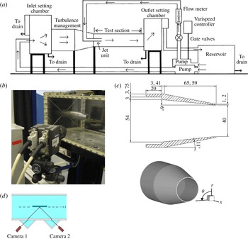
The experiments were performed in a water tunnel facility used in previous jet flow experimental research (Behrouzi & McGuirk Reference Behrouzi and McGuirk2004, Reference Behrouzi and McGuirk2006), see figure 1(a). The tunnel is of recirculating design and can accommodate both single and coaxial nozzles. The test section is 2010 mm long, 375 mm wide and 300 mm high. Perspex sidewalls as well as roof/ceiling enable non-intrusive measurement techniques to be used to measure the flow. The flow was seeded with neutrally buoyant polyamide seeding particles with a mean particle diameter of
 $20~{\rm\mu}\text{m}$
. Due to the recirculating design of the tunnel, complete seeding saturation was possible; uniform seeding density was achieved in both jet and surrounding tunnel flow,
 ${\sim}10$
particles per PIV interrogation window. An upstream contraction and turbulence management screens ensured good uniformity of any coflowing stream outside the jet; preliminary measurements showed this was uniform to within 1.25 % (Pokora Reference Pokora2009). A conical convergent nozzle was used, based on the geometry described in the study of Power et al. (Reference Power, Kerherve, Fitzpatrick and Jordan2004), and is shown in figure 1(b,c). The nozzle exit diameter (
 $D_{j}$
) was 40 mm, with internal and external face convergence angles of
 $6^{\circ }$
and
 $11^{\circ }$
and an exit plane lip thickness of 1.2 mm. To ensure the nozzle was located in the centre of the water tunnel, a supporting cross-shaped structure was used (figure 1
b) and allowed the jet axis to be aligned to within
 $1^{\circ }$
with respect to the tunnel walls.
(a) Water tunnel; (b) PIV camera and jet nozzle inside water tunnel; (c) nozzle geometry and coordinate definition; (d)
 $x{-}r$
plane 3C-PIV water jacket arrangement.

The bulk average nozzle exit velocity was
 $1~\text{m}~\text{s}^{-1}$
, giving a Reynolds number
 $\mathit{Re}_{D}=4\times 10^{4}$
. The airflow data in the literature reviewed in the Introduction have generally been taken at higher Reynolds numbers than this (typically from
 $\mathit{Re}_{D}\sim 1\times 10^{5}$
to
 ${\sim}5\times 10^{5}$
) and at Mach numbers varying from 0.3 to 0.9. However, if attention is focused on flow and, in particular, on turbulence data (as opposed to acoustic measurements), when plotted non-dimensionally no significant Reynolds number or Mach number effects were observed in any of these published studies. In addition, the experiments of Ricou & Spalding (Reference Ricou and Spalding1961) concluded that the entrainment process for turbulent free jets became independent of
 $\mathit{Re}_{D}$
above
 $2\times 10^{4}$
. The recent measurements of Fellouah, Ball & Pollard (Reference Fellouah, Ball and Pollard2009) in the jet near field (
 $x/D<30$
) supported this view, noting that, for
 $\mathit{Re}_{D}>2\times 10^{4}$
, velocity spectra in the shear layer displayed a clear inertial subrange, indicating a one-way coupling of large turbulent scales and viscosity influenced small-scale motions. Their measurements showed no significant dependency on
 $\mathit{Re}_{D}$
for the centreline mean velocity decay rate for
 $\mathit{Re}_{D}$
above
 $10^{4}$
in the near-field region studied. The peak turbulent stresses in the shear layer showed less than 5 % change for
 $\mathit{Re}_{D}$
above
 $10^{4}$
– and even then only in the immediate vicinity of the nozzle. The conclusion from these investigations is that Reynolds-number effects are predominantly associated with the transition of the near-wall flow from a wall boundary layer (which does contain a region of direct viscous-influenced flow) to a turbulent free shear layer. This process begins at the nozzle exit and takes place typically within the first one or two nozzle diameters of axial length; after that the shear layer and jet development are dominated by turbulence processes that are not directly set by molecular viscosity. Thus, the Reynolds number for the present experiment was chosen to be sufficiently high such that the measurements will be relevant to the high-
 $\mathit{Re}$
nozzle flows found in practice.
Figure 1(c) indicates the cylindrical polar (
 $x,r,{\it\theta}$
) coordinate system, with origin at the nozzle exit centreline, used to present the data. For 3C-PIV measurements, water-filled prisms were attached to the tunnel walls to ensure the optical axis of the PIV cameras was orthogonal to the first air/Perspex/water interface (figure 1
d). Placing the jet in a confined environment will affect the development of the flow to a greater or lesser extent dependent upon geometry and test conditions. A RANS-based CFD study (
 $k$
–
 ${\it\varepsilon}$
turbulence model) was undertaken (Pokora Reference Pokora2009) in order to minimise these effects. The mixing of the jet and external coflow is determined by the entrainment rate, which is controlled primarily by the ratio of jet to coflow velocities. If the flow development is to be similar to that of a free jet, this velocity ratio must be as large as possible. However, if the water tunnel coflow does not supply sufficient entrainment flow for the whole downstream development of the jet, an adverse pressure gradient is created in the tunnel that can cause flow recirculation in the external coflow. By adjusting the ratios of nozzle diameter/tunnel size and jet/tunnel velocity this confinement effect can be minimised, by ensuring a value of the Craya–Curtet number (Craya & Curtet Reference Craya and Curtet1955) such that
 $\mathit{Ct}>1.0$
. Thus if
 $U_{j}$
,
 $U_{cf}$
and
 $U_{m}$
are the jet, coflow and fully mixed bulk average velocities, and
 $D_{j}$
and
 $D_{cf}$
are the diameters of jet and coflow areas (equivalent circular area for the coflow), Ct is given by
 $$\begin{eqnarray}\mathit{Ct}=\frac{U_{m}}{\displaystyle \left[(U_{j}^{2}-U_{cf}^{2})\left(\frac{D_{j}}{D_{cf}}\right)^{2}+\frac{(U_{cf}^{2}-U_{m}^{2})}{2}\right]}.\end{eqnarray}$$
A coflow velocity of
 $0.18~\text{m}~\text{s}^{-1}$
was found to avoid any recirculation or jet-flapping-induced unsteadiness at the far downstream end of the test section. Comparison of confined water flow measurements with free jet airflow data are provided in § 3 to indicate that the data measured here are representative of turbulent subsonic free jet behaviour. Further, by providing all required boundary conditions appropriate to the present experimental set-up, comparable CFD simulations may be carried out for direct comparison with the present measurements.
2.2. Instrumentation
The PIV system used consisted of a pair of LaVision High Speed Star 4 (HSS4)
 $1024~\text{pixel}\times 1024~\text{pixel}$
resolution cameras (at 10 bit dynamic range) capable of frame rates up to 1 kHz double frames at full resolution, at which the on-board camera memory enables a sample size of 3 s, allowing a total of 3072 instantaneous vector fields to be recorded. Lenses of focal lengths from 24 to 105 mm were used, depending on the desired FoV. The light source was a New Wave double-cavity high-speed Nd/YLF Pegasus laser with wavelength 527 nm and power of
 $10~\text{mJ}~\text{pulse}^{-1}$
at a repetition rate of 1 kHz with pulse duration 6 ns. The PIV cameras and lasers were controlled by LaVision’s DaVis (v7.2) software and Programmable Timing Unit (PTU). The laser beams are fired through an optical arm followed by a divergent lens to form a laser sheet with adjustable thickness 0.5–2.5 mm. The laser head and both cameras were mounted on a Dantec Dynamics three-axis traverse enabling system alignment to
 ${\sim}0.2~\text{mm}$
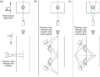
. PIV calibration used the LaVision two-level calibration plate placed within the tunnel. For 2C-PIV only a single camera is used, viewing orthogonal to the water tunnel sidewall; for stereo 3C-PIV measurements, where two cameras viewed the flow field at an oblique angle through the tunnel sidewall, water jackets with
 $45^{\circ }$
sides were fitted to the sides of the tunnel (figure 1
d) to ensure the lenses of both cameras were located parallel to the first air/Perspex boundary in order to reduce any effects incurred due to refractive index changes. Scheimpflug lenses were included to tilt the image plane with respect to the orientation of the camera lens and light sheet. This arrangement widens the focused range, although has the side effect of introducing a strong perspective distortion; the factor of magnification is also no longer constant across the complete field of view. Both of these are accounted for during image calibration. A focal length lens of 105 mm was used for 2C-PIV measurements, producing a FoV of
 $25~\text{mm}\times 25~\text{mm}$
; the rationale for this choice of small FoV size is discussed below. For 3C-PIV in an
 $x{-}r$
plane, both cameras viewed through the tunnel sidewall; if the laser sheet was oriented in the
 $r{-}{\it\theta}$
plane, one camera was placed on each side of the illuminated plane. For the
 $r{-}{\it\theta}$
orientation, the 105 mm lenses were equipped with 2× teleconverters; this, together with a viewing arrangement – i.e. with cameras and Scheimpflug lenses on either side of the light sheet plane – leads to some elongation due to perspective effects, and in the
 $r{-}{\it\theta}$
plane the FoV width was increased from 25 to 30 mm. Figure 2 displays the different orientations of the instrumentation for 2C- or 3C-PIV and in different planes.
Camera/laser locations for various measurement configurations (light sheet always in vertical plane), (a) 2C
 $x{-}r$
plane, (b) 3C
 $x{-}r$
plane, (c) 3C
 $r{-}{\it\theta}$
plane. For 3C set-up camera views through side window with water jackets.

2.3. Data definitions
The usual Reynolds decomposition is adopted to separate time-mean (statistically stationary) and fluctuating components of the instantaneous velocity field:
 $$\begin{eqnarray}U_{i}^{inst}(\underline{x}_{P},t)=U_{i}(\underline{x}_{P})+u_{i}^{\prime }(\underline{x}_{P},t),\quad \text{where }U_{i}(\underline{x}_{P})=\frac{1}{N_{samp}}\mathop{\sum }_{n=1}^{N_{samp}}U_{i}^{inst}(\underline{x}_{P},t_{n}).\end{eqnarray}$$
The time mean of any variable is calculated at the centre of each PIV interrogation window (
 $\underline{x}_{P}$
) by averaging over the total number of PIV frames sampled, as shown above for the mean velocity. Single-point Reynolds stresses are defined as usual, e.g. for the root mean square (r.m.s.) of the Reynolds normal stresses (an overbar now indicating averaging over frames):
 $$\begin{eqnarray}u_{i}^{rms}(\underline{x}_{P})=\sqrt{\overline{u_{i}^{\prime 2}}}(\underline{x}_{P}).\end{eqnarray}$$
For spatio-temporal characteristics of the turbulence, the definitions adopted for the normalised second- and fourth-order two-point, two-time correlations have been given above. Simpler correlations of interest may be obtained by setting specific values of
 $\underline{{\it\eta}}$
and
 ${\it\tau}$
, e.g. the auto-correlation function is obtained by setting
 $\underline{{\it\eta}}=0$
and the spatial correlation function by setting
 ${\it\tau}=0$
. Integral length scales may be extracted from the spatial correlations, e.g. at second-order level:
 $$\begin{eqnarray}\text{}^{k}L_{ij}(\underline{x}_{P})=\int _{0}^{\infty }R_{ij}(\underline{x}_{P},{\it\eta}_{k},0)\,\text{d}{\it\eta}_{k}\end{eqnarray}$$
where
 $k$
indicates the component of the separation vector along which integration is carried out; the streamwise integral scale is evaluated as
 $\text{}^{1}L_{11}$
and the transverse integral scale as
 $\text{}^{2}L_{11}$
. Note that in practice these integral scales are evaluated up to the first zero crossing of the correlation function (as in Fleury et al.
Reference Fleury, Bailly, Jondeau, Michard and Juve2008), and for accuracy it was always ensured that the evaluation point
 $\underline{x}_{P}$
was sufficiently far from the edge of the FoV that the correlation decreased to zero within the FoV in the direction of integration.
Similarly, the second-order correlation function may be used to analyse the fluctuating energy distribution. The energy spectrum (power spectral density PSD) may be obtained from a Fourier transform of the auto-correlation function:
 $$\begin{eqnarray}E_{ij}(\underline{x}_{P},{\it\omega})=2\int _{0}^{\infty }R_{ij}(\underline{x}_{P},0,{\it\tau})\cos ({\it\omega}{\it\tau})\,\text{d}{\it\tau}.\end{eqnarray}$$
Noise due to low sampling rates can produce noisy spectra; to avoid this, all spectra presented below were calculated as the mean of spectra at the nine interrogation cells surrounding a given location, given the fine spatial resolution used this was considered acceptable.
2.4. Data quality checks
Image processing
The standard checks to monitor the quality of the conversion of raw PIV images to vector fields were carried out. An Adaptive Multi-Pass technique was used with final cell size
 $32~\text{pixel}\times 32~\text{pixel}$
; to increase vector density, 50 % overlap of PIV cells was adopted.
Vector validation
The quality of the vector map produced was quantified and improved using the standard
 $Q$
-factor (a ‘pass’ test of
 $Q>2$
was adopted to indicate a valid vector) and ‘near-neighbour’ tests (see Westerweel et al.
Reference Westerweel, Draad, Van der Hoeven and Van Oord1996). All vectors removed were replaced to maintain a continuous field. For 2C-PIV data, the number of first-choice vectors was greater than 98 %; for 3C-PIV, this was 80 %, but the number of first- or second-choice vectors was 95 %.
Subcell filtering estimation and correction
The method of Spencer & Hollis (Reference Spencer and Hollis2005) has been used to estimate the level of turbulence energy lost due to subcell spatial filtering, to correct for this, and also to choose the most appropriate size for the PIV FoVs at various locations in the jet (shear layer growth changes the integral scale, hence permittting larger PIV interrogation window/cell sizes and FoVs at downstream locations). The size of the PIV cell effectively performs a low-pass filter on the measured displacement of the seeding particles; fluctuating energy of any scales smaller than the cell size is filtered out. Hoest-Madsen & Nielsen (Reference Hoest-Madsen and Nielsen1995) produced an estimate of this loss of turbulence in PIV measurements expressed via a predicted curve for the ratio of measured turbulence r.m.s. to true r.m.s. as a function of the ratio of PIV cell size (
 ${\rm\Delta}x$
) to the local integral scale of turbulence (
 $L$
). For example if
 ${\rm\Delta}x/L=1$
, a loss in measured turbulence of around 30 % was predicted to occur. Using this curve to correct PIV measurements is problematic, since a priori the integral length scale (and its variation across the FoV) is unknown. In addition, the Hoest-Madsen and Nielsen prediction assumed homogeneous isotropic turbulence, which is rarely the case in practice. Spencer & Hollis (Reference Spencer and Hollis2005) suggested an improved approach for turbulence correction based on: (i) a correction curve for turbulence error versus
 ${\rm\Delta}x/L$
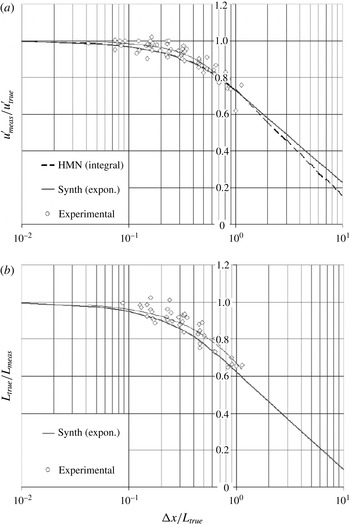
generated from measurements in shear flows (boundary layer, free shear, separated and wake flows) to avoid assumptions about the nature of the turbulence, (ii) use of an LDA technique to obtain the true r.m.s., since this does not suffer from the same spatial filtering problem and was compared with PIV measurements on a series of ever decreasing size FoVs, and (iii) calculation of the integral scale from the PIV data using (2.4), again on a series of ever-decreasing FoV size, with the most accurate value taken from the smallest FoV to create a second correction curve for the integral length scale. Figure 3 presents the two correction curves taken from Spencer & Hollis (Reference Spencer and Hollis2005). These two curve fits have been used in the present work to estimate corrected PIV-measured quantities
 $u_{meas}^{rms}$
and
 $L_{meas}$
. Note that iteration between these curves is needed, given
 $u_{meas}^{rms}$
and
 $L_{meas}$
, to complete the correction (for details, see Spencer & Hollis Reference Spencer and Hollis2005).
Subcell filtering correction curves for (a) r.m.s. and (b) integral scale (from Spencer & Hollis Reference Spencer and Hollis2005).

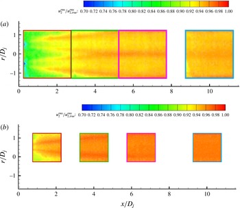
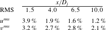
As an illustration of the use of this method, figure 4 shows the ratio between measured radial r.m.s. values taken in the present study and corrected values using the above methodology for a PIV with FoV centred on selected points in the jet shear layer at four axial locations. Two FoV sizes were explored:
 $100~\text{mm}\times 100~\text{mm}$
and
 $60~\text{mm}\times 60~\text{mm}$
; the axial r.m.s. indicated lower errors (see Pokora Reference Pokora2009), so results for radial r.m.s. are shown. The contour maps show that for the larger FoV the error is significantly larger – up to 25 % loss of energy is indicated at the first measurement location (thinnest shear layer). This error is reduced for the smaller FoV to less than 10 %. This shows the importance of adjusting the FoV size to match the local integral scale. At
 $x/D_{j}=1.5$
, tests showed that to reduce the error to less than 5 %, a FoV of
 $25~\text{mm}\times 25~\text{mm}$
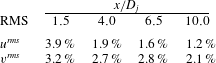
was necessary. Table 1 shows the errors evaluated using the Spencer and Hollis methodology for a FoV of
 $25~\text{mm}\times 25~\text{mm}$
for both axial and radial r.m.s., and this is the reason this FoV size was chosen for the 2C-PIV data to ensure optimum spatial and temporal resolution.
Radial r.m.s. error maps for FoV sizes: (a)
 $100~\text{mm}\times 100~\text{mm}$
, (b)
 $60~\text{mm}\times 60~\text{mm}$
.

Error levels, axial and radial r.m.s. for FoV of
 $25~\text{mm}\times 25~\text{mm}$
.
Finally, table 2 compares the spatial resolution achieved in the present experiments to the previous studies of Wernet (Reference Wernet2007), Fleury et al. (Reference Fleury, Bailly, Jondeau, Michard and Juve2008). On the basis of this, the present measurements contain significantly lower levels of spatial filtering of turbulence than in previous work.
Spatial resolution achieved in various PIV studies.

Choice of FoVs
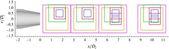
As well as considering FoV size for high accuracy, the need to measure two-point correlations at large enough separation vectors to capture the whole extent of the correlation function must be considered. Measurements were again conducted using various FoV sizes, centred on points where the correlations/length scales measured could be compared with data from literature. Sufficiently large FoVs were also required to ensure the correlations would decay to zero within the FoV in both in-plane directions (the integral length scales measured by Fleury et al. (Reference Fleury, Bailly, Jondeau, Michard and Juve2008) were used to guide this). The FoVs used are shown in figure 5 for two locations in the shear layer on the nozzle lipline upstream of potential core end (
 $r/D_{j}=0.5$
, at
 $x/D_{j}=1.5$
, 4.0), two locations near potential core end (
 $x/D_{j}=6.5$
, at
 $r/D_{j}=0.5,0$
), and two further downstream (
 $x/D_{j}=10$
, at
 $r/D_{j}=0.5,0$
). At each location five FoVs were used, varying in size from
 $25~\text{mm}\times 25~\text{mm}$
to
 $100~\text{mm}\times 100~\text{mm}$
, with data taken both at 50 Hz (for longer sampling time) and 1 kHz (for maximum temporal resolution) – in each case with 3072 samples gathered.
Location of different size FoVs within jet region.

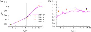
Figure 6 shows measurements of the axial r.m.s. velocity fluctuation along the jet centreline (
 $r/D_{j}=0$
) and the nozzle lipline (
 $r/D_{j}=0.5$
) for all FoV sizes. On the centreline within the potential core region, there can be no shear-generated turbulence; the measured turbulence should be no larger than at the nozzle exit (i.e. low
 ${\sim}0.01~\text{m}~\text{s}^{-1}$
) and decay downstream until the inner edge of the lipline shear layer meets the centreline. Figure 6(a), however, shows considerable and increasing apparent turbulence in the region
 $0<x/D_{j}<5$
(a feature also observed by Power et al. (Reference Power, Kerherve, Fitzpatrick and Jordan2004)). A change in gradient is seen at
 $x/D_{j}=6.3$
; this indicates the arrival of ‘true’ shear-generated turbulence on the centreline and identifies the potential core length
 $L_{PC}$
. In the
 $\mathit{Ma}=0.75$
,
 $\mathit{Re}=8\times 10^{5}$
airflow measurements of Power et al. (Reference Power, Kerherve, Fitzpatrick and Jordan2004)
 $L_{PC}$
was measured as
 $6.5D_{j}$
, providing further evidence of the marginal influence of both Mach number and Reynolds number (if this is high enough) on turbulence development in the present flow. On the centreline upstream of the potential core end the PIV system is actually measuring irrotational unsteadiness induced by the streamwise convection of large turbulent structures in the shear layer, which cause the edge of the inviscid potential core region (and hence the velocity within it) to fluctuate. Only after potential core end does the FoV size influence results, with smaller FoVs producing slightly higher r.m.s. A better indication of large FoV size causing turbulence error is seen in the lipline measurements (figure 6
b). At small
 $x/D_{j}$
the FoV size has a large effect (thin shear layer relative to FoV size); further downstream, as the integral length scale grows, less subcell filtering is evident. The data on the lipline become sensibly independent of FoV beyond
 $x/D_{j}=4$
, where the difference between FoVs of 40 mm and 25 mm is less than 3 %. On the other hand, the scatter is seen to increase at larger
 $x/D_{j}$
, since the integral time scale also grows, implying fewer statistically independent samples in the fixed sample duration (3 s).
Axial development of
 $u_{rms}$
for (a) jet centreline and (b) jet lipline.

Statistical accuracy
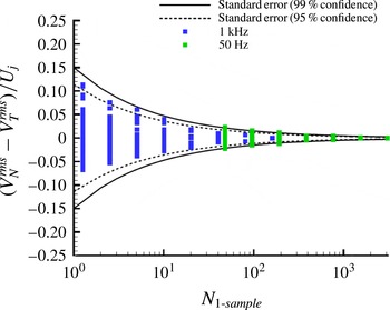
Statistical accuracy is dependent on the number of independent samples; this was the reason data were also collected at 50 Hz. Convergence is slower for locations further downstream (larger turbulence time scales) and for second-moment quantities. Figure 7 illustrates a typical example from the present measurements using different subsample sizes of the full dataset for a point on the centreline at the furthest downstream station and for the radial r.m.s. Standard error curves for 95 % and 99 % confidence limits are also included, with the convergence rate from subsampling agreeing well with these.
Statistical sampling check:
 $v_{rms}$
at
 $x/D_{j}=10.0$
,
 $r/D_{j}=0$
.

3. Results
3.1. 2C-PIV data – comparison with subsonic jet airflow data
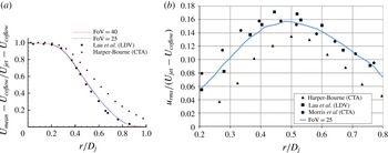
Single-point measurements were first made using 2C-PIV to provide evidence to support the use of PIV data gathered in a water flow experiment as representative of subsonic isothermal airflow jet turbulence. Measured PIV mean flow statistics in the
 $x{-}r$
plane are shown in figure 8 via radial profiles at
 $x/D_{j}=4$
of the axial mean and r.m.s. velocity compared to the LDA data of Lau et al. (Reference Lau, Morris and Fisher1979) (
 $\mathit{Re}=3\times 10^{5}{-}10^{6}$
,
 $\mathit{Ma}=0.28$
, 0.9), Morris & Zaman (Reference Morris and Zaman2010) (
 $\mathit{Re}=3\times 10^{5}$
,
 $\mathit{Ma}=0.26$
) and the HWA data of Harper-Bourne (Reference Harper-Bourne2003) (
 $\mathit{Re}=2\times 10^{5}$
,
 $\mathit{Ma}=0.18$
). The good agreement in the mean profile with airflow data at higher
 $\mathit{Re}$
indicates the behaviour of the jet shear layer is essentially unaffected by the use of water compared to airflow, the tunnel confinement, or the value of
 $\mathit{Re}$
. The PIV-measured axial turbulence r.m.s. profile also lies in between the profiles measured by Lau et al. (Reference Lau, Morris and Fisher1979), Morris & Zaman (Reference Morris and Zaman2010) and Harper-Bourne (Reference Harper-Bourne2003). The consensus dataset established by the review of many free jet data by Bridges & Wernet (Reference Bridges and Wernet2010) at various Reynolds numbers and subsonic Mach numbers indicated a peak axial r.m.s. value of 0.16 at this axial location; the present data are in good agreement with this value.
Radial profiles of (a) mean and (b) r.m.s. axial velocity at
 $x/D_{j}=4.0$
.

As noted in the Introduction, numerous airflow experiments over a range of subsonic jet Mach numbers have provided turbulence statistical information based on two-point measurements. The most important physical parameter on this category is the turbulence length scale information at locations within jet shear layers provided by various authors (Liepmann & Laufer Reference Liepmann and Laufer1947; Davies et al.
Reference Davies, Fisher and Barratt1962; Harper-Bourne Reference Harper-Bourne2003; Fleury et al.
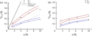
Reference Fleury, Bailly, Jondeau, Michard and Juve2008). Turbulence length scales are evaluated by integrating the measured second-order spatial correlation functions for both axial and radial fluctuations and with respect to both axial and radial separation vectors (as defined in (2.4) above). Figure 9 shows data obtained from the present 2C-PIV measurements (symbols) compared to the 2C-PIV-measured data presented in Fleury et al. (Reference Fleury, Bailly, Jondeau, Michard and Juve2008); information on the second-order correlation functions
 $R_{ij}$
measured in the present 2C-PIV study will be presented below in § 3.4. It can be seen that the values obtained from the present water flow experiments are in excellent agreement for all four length scales with the airflow data obtained using PIV and for a two subsonic Mach numbers (0,6 and 0.9) by Fleury et al. (Reference Fleury, Bailly, Jondeau, Michard and Juve2008). This provides strong support to the argument that the two-point correlations and associated turbulent structures present in low-speed water flow experiments, when suitably normalised, are identical to subsonic jet airflow characteristics.
Axial (a) and radial (b) length scales at
 $r/D_{j}=0.5$
Red and blue lines indicate range of data in experiments of Fleury et al. (Reference Fleury, Bailly, Jondeau, Michard and Juve2008).

This examination of single-point and two-point turbulence statistics was considered sufficient to demonstrate that the combination of a water flow experiment and PIV measurements at 1 kHz (with a suitably chosen small FoV) can achieve spatial and temporal resolution comparable to the high temporal resolution HWA methods as used in subsonic airflow experiments, and can thus deliver data on the important turbulence correlations which characterise the aerodynamic noise source.
3.2. 3C-PIV data – preliminary measurements
The PIV system parameters (FoV size, vector validation, number of frames etc.) were optimised as described above using 2C-PIV for the
 $x{-}r$
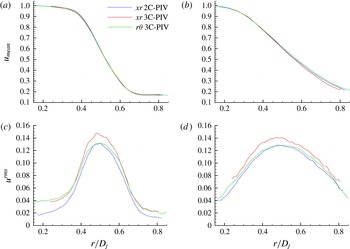
plane velocity field. When moving to 3C-PIV, measurements were first carried out to judge the quality of the 3C data compared to the standard established after 2C-PIV optimisation, since some deterioration and increase in measurement error was to be expected. Figure 10 shows a comparison of 3C-PIV and 2C-PIV single-point data for mean axial velocity (a,b) and axial r.m.s. (c,d) at various axial locations. In general the 2C- and 3C-PIV data for the mean velocity are in very good agreement. For measurements of the turbulent fluctuations it would be expected that 3C data taken with the laser sheet in the
 $x{-}r$
plane, when the streamwise velocity is an in-plane component, would be more accurate than 3C measurements with the laser sheet in the
 $r{-}{\it\theta}$
configuration (see figure 2 above), when the streamwise velocity is an out-of-plane component. In addition to this, as noted in § 2.2 above, the
 $r{-}{\it\theta}$
plane FoV is actually 20 % larger than the
 $x{-}r$
plane FoV, which would be expected to lead to increased loss of turbulence. It is therefore surprising that in figure 10, whilst the measurements of r.m.s. with both 2C- and 3C-PIV systems are fairly close, the
 $r{-}{\it\theta}$
data are in better agreement with the 2C measurements than the
 $x{-}r$
data, which show a 20 % increased peak value compared to 2C data. This arouses suspicion that increased noise in the 3C data was compensating in the
 $r{-}{\it\theta}$
measurements for extra turbulence loss, and thus showing false ‘good’ agreement with the 2C data.
Radial profiles: axial mean (a,b) and r.m.s. (c,d) at
 $x/D=1.5$
(a,c), 4.0 (b,d) – different PIV configurations.

Examination of data for the instantaneous velocity vector field produced by 3C-PIV
 $x{-}r$
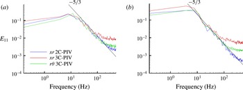
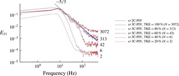
plane measurements indicated a larger number of spurious vectors that ‘survived’ the vector post-processing filter than in 2C-PIV data taken in the same plane and with the same PIV set-up (an example of this is presented later). This reinforced the suspicion that the 3C data contained a noise source not in the 2C data, and that this was occurring at high frequencies. Although stronger filtering helped to reduce the number of spurious vectors, some remained, and it was felt stronger filtering was too crude an approach, since this may adversely affect the energy content in frequency regions which were not affected by increased instrumentation noise. An alternative method for removal of possible high-frequency noise was therefore required. The method adopted was suggested by close examination of the 2C and 3C measured frequency spectra. Figure 11 presents 2C-PIV and 3C-PIV PSD measurements for the axial velocity fluctuation at a point in the centre of the shear layer and at two axial locations; the smallest 25 mm FoV data are shown. It is clear that, whilst the 2C data follow a
 $-5/3$
equilibrium energy cascade well for two decades of energy decrease, at frequencies greater than 100 Hz there is evidence of increased noise contamination in the 3C-PIV data causing high-frequency ‘lift’, with the measured data lying above the equilibrium line. This is particularly strong in the 3C-PIV data for the
 $x{-}r$
plane and becomes stronger with downstream distance, where any FoV-size-based measurement errors become weaker rather than stronger. A POD-based filter method was therefore developed to correct for this high-frequency contamination, as outlined in the following section.
PSD of fluctuating axial velocity:
 $r/D_{j}=0.5$
and
 $x/D_{j}=1.5$
(a) and 10.0 (b).

3.3. 3C-PIV filtering/correction method
It is clearly important that any correction method should not affect the raw data in spectral regions not believed to be contaminated by noise. Any filtering should only remove spurious contributions to the fluctuating energy. Proper orthogonal decomposition was an obvious possible approach, since this orders spatial modes in terms of decreasing contribution to the overall energy captured. Time-resolved POD (Weitao, Yasuhiko & Haruki Reference Weitao, Yasuhiko and Haruki2003) uses the time-series information at each 3C-PIV interrogation cell to produce an optimal energy-based decomposition into modes. By adopting a low-energy modal cutoff filter, it is possible to filter high-frequency noise contributions. Proper orthogonal decomposition is first used to analyse the velocity field and identify a hierarchy of spatial modes; from this information a series of velocity fields may be reconstructed containing, for example, only the first
 $N$
modes (larger
 $N$
thus corresponds to weaker filtering). An example of such a reconstruction is provided in figure 12 using different numbers of POD modes, from just the first 2 then 6, 42, 313, and finally all 3072 modes; the fraction of the total kinetic energy these contain is also shown in figure 12.
Effect of POD mode number on reconstructed PSD (blue – 2C-PIV).

Figure 12 illustrates clearly that if a large amount of energy is filtered (small
 $N$
) then the original PSD is altered not only in the high-frequency region where spurious high-frequency lift is suspected (the 2C-PIV spectrum was used to identify this), but also at frequencies believed to be accurate (good agreement between 3C-PIV and 2C-PIV data). However, if a larger
 $N$
is selected (say 313), filtering only 20 % of the original energy, then the resulting PSD is very close to the 2C-PIV PSD over practically the whole range of temporally resolved frequencies. The original 3C-PIV spectrum (
 $N=3072$
) departs from the 2C-PIV data at
 ${\sim}50~\text{Hz}$
; if the 20 % POD filtered spectrum is used, this is close to the 2C-PIV spectrum up to
 ${\sim}300~\text{Hz}$
, a sixfold improvement.
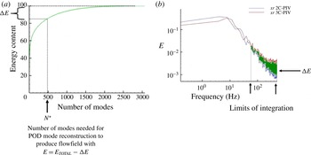
The method adopted was to select a number
 $N^{\ast }$
of POD modes, where
 $N^{\ast }$
was defined to maximise the cumulative energy fraction and provide the best fit to the 2C-PIV spectrum. The reconstructed energy content may be viewed as original energy minus a fraction assumed to be high-frequency (spurious) noise.
 $N^{\ast }$
was varied for each point within the FoV and for each location in the jet. An illustration of the method is provided in figure 13. The amount of spurious energy to be removed (
 ${\rm\Delta}E$
) is defined by two limits of integration in frequency space (figure 13
b). The upper limit was set to the highest resolved frequency (500 Hz); the lower limit was set by the value of
 $N^{\ast }$
chosen as described above. Note that departure from a
 $-5/3$
spectrum could have been used and would have produced similar results.
Illustration of POD correction method.

Using this method, table 3 shows for various points the amount of spurious energy identified which was typically removed from the
 $x{-}r$
plane 3C-PIV measurement to generate corrected 3C-PIV spectra;
 $r{-}{\it\theta}$
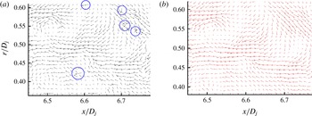
planes treated were similarly. To illustrate the consequence of this procedure on instantaneous frames of PIV vectors, figure 14 shows, for the plane
 $x/D_{j}=6.5$
: (a) the original vector field captured by the 3C-PIV and (b) the reconstructed field using the described POD filtering.
Spurious energy content identified and removed from 3C-PIV measurements.

Example of instantaneous vector fields at
 $x/D_{j}=6.5$
, (a) original, (b) original
 $+$
POD correction.

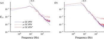
Figure 14(a) contains the spurious vectors not removed during normal PIV vector post-processing (shown circled), which are the main source of the noise in the ‘raw’ 3C-PIV spectrum. Modification of the post-processing parameters to remove these was explored, but caused undesirable removal of energy in PSD regions which were in good agreement with the 2C-PIV data. Figure 14(b) shows the result of the POD correction method described – all spurious vectors have been removed and the larger coherent structures have become more defined. Figure 15 presents the effect of filtering on the PSD of the
 $N^{\ast }$
-mode reconstructed field. The reduction in the high-frequency noise is exactly as desired, and comparison between the 2C-PIV spectra and the filtered spectra (labelled 3C-
 $\text{PIV}^{\ast }$
) is excellent for all locations within the important shear layer region. All 3C-PIV
 $x{-}r$
and
 $r{-}{\it\theta}$
plane data have been filtered using this method to produce the results reported below.
Power spectra of axial velocity-comparison of 2C-PIV, 3C-PIV and
 $3\text{C}^{\ast }$
-PIV (a)
 $x/D_{j}=1.5$
,
 $r/D_{j}=0.5$
, (b)
 $x/D_{j}=10.0$
,
 $r/D_{j}=0.5$
.

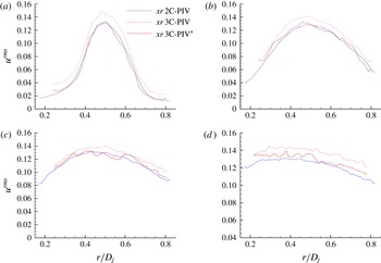
Radial profiles of axial r.m.s., as discussed above in figure 11, were examined again using the 3C-
 $\text{PIV}^{\ast }$
dataset at all measured shear layer locations. Figure 16 shows the comparison between 2C-PIV, original 3C-PIV and filtered 3C-
 $\text{PIV}^{\ast }$
data. The improvement in the agreement between 2C and 3C∗ data provides strong evidence in support of the POD-based correction methodology. At
 $x/D_{j}=1.5$
, the
 $3\text{C}^{\ast }$
profile lies almost exactly on the 2C profile; further downstream improved agreement is noticeable. Increased statistical noise is caused by the removal of some data, but the filtered results are still a significant improvement on the single-point second-order turbulence statistics.
Radial profiles of axial RMS fluctuations
 $x/D_{j}=$
(a) 1.65, (b) 4.0, (c) 6.5, (d) 10.0.

3.4. Spatio-temporal correlation functions
Second-order
 $R_{11}$
spatio-temporal plots in the
 $x{-}r$
plane were produced for all four measurement stations within the jet shear layer (
 $r/D_{j}=0.5$
); emphasis has been placed on shear layer locations, since examination of measurements on the jet centreline showed much better agreement between 3C-PIV and 3C-
 $\text{PIV}^{\ast }$
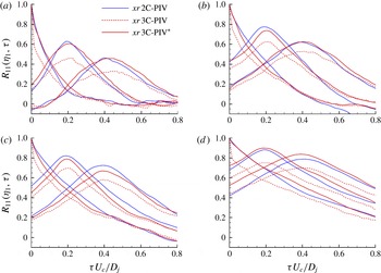
results (see Pokora Reference Pokora2009). Comparisons between 2C-PIV, 3C-PIV and filtered 3C-
 $\text{PIV}^{\ast }$
data are shown in figure 17 for three values of streamwise separation:
 ${\it\eta}_{1}=0D_{j}$
,
 $0.2D_{j}$
,
 $0.4D_{j}$
. The time axis is non-dimensionalised by a characteristic time scale of the mean flow based on jet nozzle exit diameter and velocity. Whilst the 3C-PIV data shows significant discrepancies from the 2C-PIV data, the agreement between 2C-PIV and 3C-
 $\text{PIV}^{\ast }$
curves is much improved. The peak amplitude decay rate and the peak location shifts indicate the eddy convection velocity is in good agreement – in fact this is true for both 3C-PIV datasets. There is, as expected, a large underestimate of the peak correlation magnitude value in the original 3C-PIV measurements. The close fit of 2C-PIV and 3C-
 $\text{PIV}^{\ast }$
correlation functions shows that the stereoscopic technique, with the addition of the POD filter/correction procedure, can produce correlation function curves as accurate as the 2C-PIV data, but extends the possible measurement capability to all three velocity components. On the basis of this evidence, this filtering methodology has been used for all further 3C-
 $\text{PIV}^{\ast }$
data presented.
 $R_{11}$
plots with axial separation – 2C-PIV, 3C-PIV and 3C-
 $\text{PIV}^{\ast }$
results at
 $x/D_{j}=$
(a) 1.64, (b) 4.0, (c) 6.5, (d) 10.0.

To assess the quantitative accuracy of the present PIV measurements for two-point quantities, second- and fourth-order space–time correlation curves for streamwise, radial and circumferential separations were constructed. This was done principally for the location (
 $4D_{j}$
,
 $0.5D_{j}$
,
 $0^{\circ }$
) in the nozzle lipline shear layer, which coincides with the measurement location chosen in Harper-Bourne’s (Reference Harper-Bourne2003) HWA data (labelled as CTA in the figures below). This dataset was chosen as it includes not only
 $R_{11}$
but also
 $R_{11,11}$
measurements for all three separation vector components. Note that for radial and azimuthal separation correlations, a constant axial separation of
 $0.1D_{j}$
(radial) or
 $0.05D_{j}$
(azimuthal) between the two points had to be included in the HWA study to avoid probe interference. This separation was also used in the 3C-
 $\text{PIV}^{\ast }$
radial evaluation to provide a direct comparison, but it was not possible to do so for the PIV azimuthal correlation measurement. In addition to this study, a location at the narrowest point in the shear layer measured (
 $1.5D_{j}$
,
 $0.5D_{j}$
,
 $0^{\circ }$
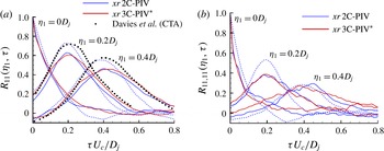
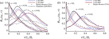
) was chosen to observe FoV size effects at the most challenging location, as well as comparison to other HWA and PIV measurements available. Results are given in figures 18–21; in all figures the horizontal axis has been evaluated using a constant convection velocity
 $U_{c}=0.6U_{j}$
– this allows differences between the actual convection velocities in different datasets to be seen more readily.
 $R_{11}$
and
 $R_{11,11}$
plots for axial separations at
 $x/D_{j}=1.5$
,
 $r/D_{j}=0.5$
. Solid lines –
 $25~\text{mm}\times 25~\text{mm}$
FoV, dashed lines –
 $40~\text{mm}\times 40~\text{mm}$
FoV.

 $R_{11}$
and
 $R_{11,11}$
plots for axial separations at
 $x/D_{j}=4.0$
,
 $r/D_{j}=0.5$
.

 $R_{11}$
and
 $R_{11,11}$
plots for radial separations at
 $x/D_{j}=4.0$
,
 $r/D_{j}=0.5$
.

 $R_{11}$
and
 $R_{11,11}$
plots for azimuthal separations at
 $x/D_{j}=4.0$
,
 $r/D_{j}=0.5$
.

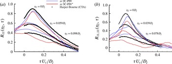
Figure 18, showing data taken close to the nozzle exit, provides conclusive evidence that the similarity of turbulence information between water and airflow experiments also extends to the correlation functions. For
 $R_{11}$
, direct comparison is made with HWA data (Davies et al.
Reference Davies, Fisher and Barratt1962, labelled CTA) as well as with 2C-PIV (two FoV sizes) and 3C-
 $\text{PIV}^{\ast }$
results. It is at this location, where the shear layer is very thin, that the PIV FoV size is most important. Figure 18(a) shows that the larger FoV (which contains more subcell filtering) gives higher peak amplitudes, but this is certainly a fortuitous and erroneous result. The agreement between the eddy convection velocities from the various experiments is seen to be good by the match in peak correlation locations at all separation values. The 2C- and 3C-
 $\text{PIV}^{\ast }$
data are in very good agreement with each other and with the HWA data (although the PIV data show reduced peak amplitude with separation). The decrease in peak value with separation distance indicates the large-scale mixing causes a ‘non-frozen’ nature of the shear layer turbulence, and the growth in correlation function width with increasing
 ${\it\eta}_{1}$
shows the growth in eddy size. There are no other measurements to compare with the fourth-order correlation at this location. The fourth-order function displays a more rapid decay in both space and time, noted by Harper-Bourne (Reference Harper-Bourne2003) as being consistent with the greater frequency content relative to second-order quantities. The agreement between the two 25 mm FoV results (2C-PIV, 3C-
 $\text{PIV}^{\ast }$
) is very good for
 $R_{11,11}$
.
Figure 19 presents similar
 $R_{11}$
and
 $R_{11,11}$
functions with axial separation, but at
 $x/D_{j}=4.0$
. Comparison with HWA results for
 $R_{11}$
is of similar quality as at the upstream station. The combined LDA/PIV method of Chatellier & Fitzpatrick (Reference Chatellier and Fitzpatrick2005) shows considerably inferior performance compared to the PIV-only technique. Close inspection of PIV and HWA data shows a slightly higher eddy convection velocity for PIV. The HWA peak amplitudes for
 $R_{11}$
are again greater than with PIV, but this difference is in fact reduced for
 $R_{11,11}$
, where PIV/HWA agreement is very good at all axial separations.
The effect of radial separation is illustrated in figure 20. For
 $R_{11}$
, the time to the peak location decreases as
 ${\it\eta}_{2}$
increases, the shifted point moving radially inwards across the shear layer, indicating a phase shift. For
 $R_{11,11}$
, agreement is very good, with the peak occurring close to zero time for small
 ${\it\eta}_{3}$
separations, as observed in the HWA data. The PIV/HWA agreement for the fourth-order components is not quite as good as for second-order quantities. Note the fact that the peak values at zero
 ${\it\eta}_{2}$
are not unity is caused by the fact that an axial separation of
 $0.1D_{j}$
has had to be included in evaluating
 $R_{11}$
and
 $R_{11,11}$
to match the HWA configuration as noted above; thus the
 ${\it\eta}_{2}=0D_{j}$
correlation is the same as the correlation for
 ${\it\eta}_{1}=0.1D_{j}$
.
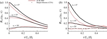
The effect of azimuthal separation is presented in figure 21; for
 $R_{11}({\it\eta}_{3},{\it\tau})$
, the alignment of HWA and PIV data is very good; this is also the case for
 $R_{11,11}({\it\eta}_{3},{\it\tau})$
, although the zero comparison shows greatest discrepancy – this is probably to a large extent caused by the neglect of the small axial separation used in the HWA data in the PIV measurement. These azimuthal correlations are significantly flatter than the axial or radial correlations for quite small increases in the separation vector; this is consistent with the axisymmetric nature of the jet flow.
Since this is perhaps the first time that PIV and HWA measurements for spatio-temporal correlations have been directly and comprehensively compared (certainly the case for all separation components for both second- and fourth-order components), it is worthwhile providing a summary overview of the PIV performance. In general, both techniques have advantages and disadvantages. Both methods contain error sources problematic for measuring the quantities of interest here. HWA has high temporal resolution, but use of anti-aliasing techniques can lead to increased correlation peak magnitudes. Planar optical measurement techniques such as PIV more conveniently allow the visualisation of correlation functions for components other than the axial velocity and for larger ranges of the separation vector than probe-based techniques. However, PIV is subject to subcell filtering and spurious vector instrumentation noise, which can cause reduced correlation peak magnitudes. As illustrated in the present study, these can be controlled using smaller FoVs, although this then places some limitations on the extent of separation vector possible. Nevertheless, it is believed that the correct quantitative behaviour of the present PIV data has been adequately demonstrated by the above HWA/PIV comparisons. To balance the slight fall-off in accuracy, PIV offers the opportunity to measure more components of
 $R_{ij}$
and
 $R_{ij,kl}$
, it is this potential which was exploited next in the present study.
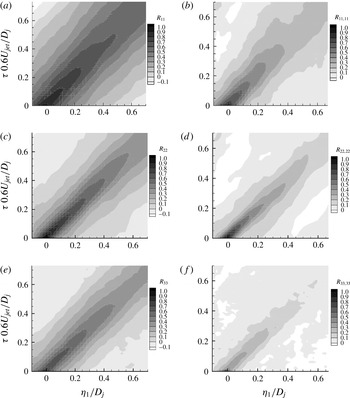
Existing data on two-point correlation maps for jet flows has concentrated on axial separation distance/time delay maps. Figure 22 shows such maps extracted from the present 3C-
 $\text{PIV}^{\ast }$
results for the point (
 $4D_{j}$
,
 $0.5D_{j}$
,
 $0^{\circ }$
). Because of the quality of the present measurements, maps for both second- and fourth-order components can be included. The diagonal trajectory of the peak correlation value allows the eddy convection velocity to be estimated; figure 22 shows that this is essentially the same (
 $0.6U_{j}$
) for all correlation components shown, and for both second- and fourth-order quantities.
Second- and fourth-rank tensor components – spatio-temporal correlation maps at (
 $4D_{j}$
,
 $0.5D_{j}$
,
 $0^{\circ }$
); (a)
 $R_{11}$
; (b)
 $R_{11,11}$
; (c)
 $R_{22}$
; (d)
 $R_{22,22}$
; (e)
 $R_{33}$
; (f)
 $R_{33,33}$
.

The high quality of the fourth-order components is particularly noticeable; the only example found in the literature for the fourth-order correlation, and
 $R_{11,11}$
only, is that of Bridges & Wernet (Reference Bridges and Wernet2003), where the trajectory was difficult to discern because of the extremely high noise level. The fourth-order maps are narrower than the second-order, as expected from the faster decay rates noted above; for both
 $R_{ij}$
and
 $R_{ij,kl}$
, the axial component displays larger regions of high correlation, extending further along the trajectory compared to radial and azimuthal components. Maps such as these allow evaluation of Lagrangian-evaluated quantities, often used in aeroacoustic models based on the use of a frame of reference moving with the eddies, as suggested by Lighthill (Reference Lighthill1952, Reference Lighthill1954). For example, the Lagrangian length scale
 $\text{}^{k}L_{ij}^{L}$
, is defined as the spatial separation at which the correlation decays to
 $1/e$
of its initial value in a moving frame of reference (i.e. along the eddy convection velocity axis). This quantity has been evaluated from the correlation maps shown in figure 22 and may be compared with HWA data from Harper-Bourne (Reference Harper-Bourne2003) for both second- and fourth-order Lagrangian length scales. For axial velocity and all three directions this comparison is shown in tables 4 and 5.
Comparison of second-order Lagrangian length scales of axial velocity.

Comparison of fourth-order Lagrangian length scales of axial velocity.

The comparison between HWA and PIV results is excellent; the anisotropy of the length scales is reproduced very well, with an order of magnitude difference between axial and transverse components at second-order, with a similar but somewhat smaller factor at fourth-order.
An alternative presentation of the data is to plot correlation maps in physical space, as done by Fleury et al. (Reference Fleury, Bailly, Jondeau, Michard and Juve2008), although for
 ${\it\tau}=0$
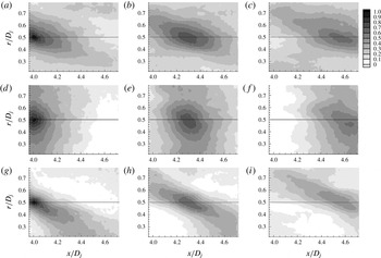
only. Figures 23 and 24 display second- and fourth-order correlation maps in the
 $x{-}r$
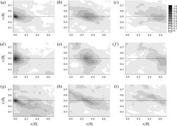
plane, with the present investigation extending the dataset to various time delays and all three velocity components. For the second-order correlations (figure 23), the elongated elliptical shape of the axial component compared to the more circular shape of the radial component is clear to see, and this has also been observed in Fleury et al. (Reference Fleury, Bailly, Jondeau, Michard and Juve2008). The circular shape tends towards elliptic at larger delay times. Figure 23 extends this information to include the
 $R_{33}$
component; this is initially similar to
 $R_{22}$
, although narrower, but becomes elliptical more quickly than
 $R_{22}$
as delay time increases. The close-to-axial trajectory of the peak value for all three components is very noticeable. A visual assessment of the quality (low spurious noise levels) of the PIV correlation maps shows well-defined edges to the correlation contours and a constant zero-background correlation level, indicating low noise levels and high quality.
Second-order spatio-temporal correlations at (
 $4D_{j}$
,
 $0.5D_{j}$
,
 $0^{\circ }$
) (a–c)
 $R_{11}$
, (d–f)
 $R_{22}$
, (g–i)
 $R_{33}$
;
 ${\it\tau}U_{c}/D_{j}=0$
(a,d,g), 0.3 (b,e,h), 0.6 (c,f,i).

Fourth-order spatio-temporal correlations at (
 $4D_{j}$
,
 $0.5D_{j}$
,
 $0^{\circ }$
): (a–c)
 $R_{11,11}$
, (d–f)
 $R_{22,22}$
, (g–i)
 $R_{33,33}$
;
 ${\it\tau}U_{c}/D_{j}=0$
(a,d,g), 0.3 (b,e,h), 0.6 (c,f,i).

This low noise level trend continues when examining similar plots for the fourth-order correlations of axial fluctuation with axial separation (i.e.
 $R_{11,11}(\underline{x},{\it\eta}_{1},{\it\tau})$
), as shown in figure 24. The more compact nature of the higher-order correlations is very well illustrated in these plots. Once again it is noteworthy that low noise levels are retained for the fourth-order correlation, although faster deterioration is visible compared to the second-order plots in figure 23.
The availability of measurements to guide aeroacoustic modelling has until recently been restricted to the axial component only. Models have therefore generally made the assumption that all components of
 $R_{ij,kl}$
may be related to
 $R_{11,11}$
by simple constant ratios. The present data cover enough components of
 $R_{ij,kl}$
to allow this assumption to be examined. Although this fourth-rank tensor contains a total of 81 components, the symmetry between tensor indices reduces the number of independent components to 36 – and if emphasis is placed on the peak amplitudes at zero space and time separations, then this number reduces further to 21. The present measurements allow the relative peak amplitudes at zero values of
 $(\underline{{\it\eta}},{\it\tau})$
for all six second-order (relative to
 $R_{11}$
) and all 21 fourth-order (relative to
 $R_{11,11}$
) independent components to be examined. Once again it is useful to start by comparing the PIV-measured data with what is available from HWA measurements. Morris & Zaman (Reference Morris and Zaman2010) have used cross-wire HWA measurements to evaluate three components of
 $R_{ij,kl}$
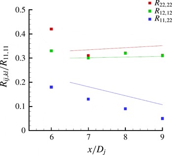
in the shear layer and along the jet centreline. Comparison is provided in figure 25 between this data and the present PIV results for the region just downstream of the end of the potential core, with generally good agreement. Another assumption made in aeroacoustic modelling is that the relative amplitudes are independent of streamwise position. Figure 25 shows this is not true for all components in this comparison, particularly for the (
 $11,22$
) component. Since the local flow structure alters from that of an annular shear layer to that of a self-similar jet beginning at the potential core end, it is perhaps not so surprising that these ratios vary with
 $x$
.
Comparison of PIV data (symbols) with HWA data (Morris & Zaman Reference Morris and Zaman2010) (lines) for fourth-order peak correlation relative amplitudes along jet centreline.

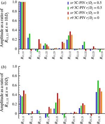
Figures 26 and 27 provide full coverage of all relevant
 $R_{ij}$
and
 $R_{ij,kl}$
relative peak amplitudes. For
 $R_{ij}$
(the point (
 $4D_{j}$
,
 $0.5D_{j}$
,
 $0^{\circ }$
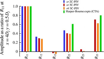
) is shown) good comparison is obtained between different PIV measurements, and the agreement with HWA is reasonable; the ratios of
 $R_{11}~R_{22}$
and
 $R_{33}$
reflect the anisotropy of turbulence in a shear layer.
Comparison of second-order peak amplitudes relative to
 $R_{11}$
for PIV and HWA results.

Comparison of fourth-order amplitudes relative to
 $R_{11,11}$
for PIV results.

For
 $R_{ij,kl}$
, data is presented at
 $x/D_{j}=10.0$
, but both shear layer (
 $r/D_{j}=0.5$
) and centreline (
 $r/D_{j}=0$
) locations are now included. One significant result is that of the possible 21 magnitudes, in the important shear layer region only six are significant, with the rest smaller by comparison; these components are:
 $R_{11,11}$
,
 $R_{11,12}$
,
 $R_{12,12}$
,
 $R_{13,13}$
,
 $R_{22,22}$
and
 $R_{33,33}$
. Such data is extremely useful for calibration of noise source models, as shown already by Karabasov et al. (Reference Karabasov, Afsar, Hynes, Dowling, McMullan, Pokora, Page and McGuirk2010).
As noted above a common assumption about the absolute correlation amplitudes is that the relative amplitudes are independent of axial position, and this was partially examined above for the jet centreline. Figure 28 shows the relative amplitude for some major
 $R_{ij,kl}$
components at several axial locations along the nozzle lipline.
Axial development of fourth-order correlation relative amplitudes along shear layer.

The assumption seems to be much more acceptable for shear layer locations, with all correlation components showing little variation with axial location from the nozzle exit to the end of the potential core (more variation seen in
 $R_{11,11}$
but still reasonable). One possible reason for this is that, unlike the centreline region considered in figure 25, once the local characteristics of the lipline flow have adjusted to the transition from a boundary layer to a shear layer, the self-similar nature of the flow means that the turbulent structures change little with downstream distance.
3.5. Approximation of fourth-order correlations via products of second-order correlations
The nature of the fourth-order two-point space–time correlation in representing the fundamental source of turbulence-generated noise means that its modelling lies at the heart of conventional acoustic analogies. Since
 $R_{ij,kl}$
has until recently defied attempts to measure it directly, at least for the vast majority of its many components, then most modelling approaches have been based on assumptions that the fourth-rank tensor can be approximated in terms of second-rank tensor expressions. Millionshchikov (Reference Millionshchikov1941) (see also Batchelor Reference Batchelor1953) was the first to propose a relationship between fourth-order and second-order velocity correlations, based on an assumption of a ‘quasi-Gaussian’ (or quasi-normal) joint probability density function between velocity components. Based on this assumption, this yields:
 $$\begin{eqnarray}\overline{u_{i}^{\prime }u_{j}^{\prime }u_{k}^{\prime }u_{l}^{\prime }}\approx \overline{u_{i}^{\prime }u_{j}^{\prime }}\cdot \overline{u_{k}^{\prime }u_{l}^{\prime }}+\overline{u_{i}^{\prime }u_{k}^{\prime }}\cdot \overline{u_{j}^{\prime }u_{l}^{\prime }}+\overline{u_{i}^{\prime }u_{l}^{\prime }}\cdot \overline{u_{j}^{\prime }u_{k}^{\prime }}.\end{eqnarray}$$
Whilst there is evidence in support of the quasi-normal approximation for single-point correlations (although mainly in simple turbulent flow such as grid turbulence), its extension to two-point statistics is less easy to justify; Morris & Zaman (Reference Morris and Zaman2010) argue that its extension to jet shear flow turbulence is problematic. Bridges & Wernet (Reference Bridges and Wernet2003) have attempted to use their direct measurements of
 $R_{11,11}$
and
 $R_{22,22}$
to assess the correctness of the quasi-normal approximation, but, as noted above, their fourth-order measurements suffered so badly from noise and scatter that drawing firm conclusions from this comparison was virtually impossible. The high quality and comprehensive nature of the present measurements encouraged an exploration of the quality of the quasi-normal approximation using the present data.
Thus, using the definition of
 $R_{ij,kl}$
given above in (1.3), the quasi-Gaussian approximation to
 $R_{ij,kl}$
may be written as follows:
 $$\begin{eqnarray}R_{ij,kl}^{QG}(x,{\it\eta},{\it\tau})=\frac{\overline{u_{i}^{\prime }(A)u_{k}^{\prime }(B)}\cdot \overline{u_{j}^{\prime }(A)u_{l}^{\prime }(B)}+\overline{u_{i}^{\prime }(A)u_{l}^{\prime }(B)}\cdot \overline{u_{j}^{\prime }(A)u_{k}^{\prime }(B)}}{[\overline{u_{i}^{\prime 4}}(A)\cdot \overline{u_{j}^{\prime 4}}(A)\cdot \overline{u_{k}^{\prime 4}}(B)\cdot \overline{u_{l}^{\prime 4}}(B)]^{1/4}-[\overline{u_{i}^{\prime 2}}(A)\cdot \overline{u_{j}^{\prime 2}}(A)\cdot \overline{u_{k}^{\prime 2}}(B)\cdot \overline{u_{k}^{\prime 2}}(B)]^{1/2}}.\end{eqnarray}$$
Note that that the PIV-measured quantities have been retained in the denominator used to non-dimensionalise this expression so that inconsistencies in the quasi-Gaussian approximation may be more readily revealed.
Figure 29 first examines the validity of the quasi-normal approximation for the principal component
 $R_{11,11}$
and four points in the jet shear layer. The overlay between the PIV-measured
 $R_{11,11}$
curves with varying axial separation and time delay and the
 $R_{11,11}^{QG}$
approximation is in general reasonable, but non-negligible discrepancies are revealed. The quasi-normal approximation fails to pick up any negative loops in the correlation and, with increasing axial separation, an overestimation in the magnitude is observed. The approximated correlations also display values at zero separation above unity, which is a further indication of error.
Comparison between measured and quasi-normal approximation of
 $R_{11,11}$
; (a)
 $x/D_{j}=1.5$
; (b)
 $x/D_{j}=4$
; (c)
 $x/D_{j}=6.5$
; (d)
 $x/D_{j}=10$
.

It is clear that it is not appropriate to focus attention just on
 $R_{11,11}$
; the comparison of relative amplitudes shown in figure 27 illustrates the presence of several other important contributions. Figure 30 shows the comparison of directly measured and quasi-normal approximated quantities for the absolute amplitudes at zero spatial and temporal separations for the six largest components in the
 $x{-}r$
plane (2C-PIV data are used here) at four shear layer locations. The previously observed overestimation of the dominant
 $R_{11,11}$
component is seen again, but the agreement for the relative magnitude of the different correlation components is rated as good, providing direct evidence for the first time for multiple components on the accuracy of the quasi-normal approximation. In general, the agreement is encouraging, but given the doubts expressed on the applicability of this approximation in shear flows (Morris & Zaman Reference Morris and Zaman2010), it would be better if alternative, more generally valid approximations such as the generalised shell model recently proposed by Afsar (Reference Afsar2012) were also compared against the present measurements.
Comparison between measured and quasi-normal approximation of
 $R_{ij,kl}$
in
 $x{-}r$
plane shear layer:
 $x/D_{j}=$
(a) 1.5, (b) 4.0, (c) 6.5, (d) 10.0.

4. Concluding remarks
The focus of the present work has been the need to obtain more detailed information about the fourth-order two-point two-time spatio-temporal correlation
 $R_{ij,kl}$
, which is the major source of turbulence-generated noise in jets. Attempts to provide measurements of the many individual components of this in subsonic airflow experiments have proven problematic. An alternative approach has been followed in the present work, based on the assumption that the characteristics of this turbulence correlation are – at the high Reynolds numbers of practical relevance – not strongly affected by Reynolds number. In addition, for the subsonic Mach numbers of prime interest, direct compressibility effects on the turbulence structure are minimal due to low convective Mach number. On this basis a water flow rather than an airflow experiment has been conducted, since the difference in kinematic viscosity between water and air means that the temporal scales of the turbulence which have to be resolved reduce by a factor of
 ${\sim}15$
, facilitating the measurements of many more components of
 $R_{ij,kl}$
than previously possible. This practice limits the applicability of the dataset produced to subsonic isothermal jets; similar measurements in high-speed and heated jets will require substantial further progress in the spatial/temporal resolution capabilities of PIV.
Stereoscopic PIV measurements were conducted in an axisymmetric turbulent jet within a water tunnel facility. Thorough comparison with existing data using both HWA and PIV in airflow experiments over a range of subsonic Mach numbers provided strong evidence that the measured turbulence structure was closely representative of high subsonic jet shear layers. An important aspect of the present work is the close attention paid to spatial filtering and the associated loss of measurement accuracy for turbulence components due to large PIV FoV size relative to local integral scales of turbulence. The correction methodology of Spencer & Hollis (Reference Spencer and Hollis2005) was adopted to identify appropriate PIV FoV sizes to avoid subcell turbulence errors, but also measure two-point correlations over large separation distances. Comparison with single-point data from other studies was shown to be good, with turbulent integral length scales estimated from the present water flow PIV measurements matching well those obtained from airflow experiments.
Second- and fourth-rank tensor spatio-temporal correlations have been evaluated from the present measurements and were shown to be of comparable accuracy to previous HWA results, both near the nozzle exit (where the integral length scale is small) and further downstream. Implementation of a POD analysis and its use as a low-pass filter was shown to be necessary when conducting 3C-PIV measurements. The POD-based correction method was demonstrated as a valid method for filtering 3C-PIV data containing high-frequency noise. The low-energy (i.e. high-frequency) POD-based filter acted in a similar fashion to the anti-aliasing filter used for hot-wire probes, allowing for more accurate spectral data.
In addition to validating the stereoscopic 3C-PIV against HWA results (for the first time for multiple fourth-order components), whole-field visualisation, for all three velocity components, via spatio-temporal correlation maps proved possible. The data obtained are ideal for validating proposed models of
 $R_{ij,kl}$
for use in jet noise prediction. To date many of these models have made use of the quasi-normal approximation to relate fourth-order correlations to second-order; the present data showed this approach to be reasonable, but also to contain several regions of discrepancy. The data presented could profitably be used to calibrate models of
 $R_{ij,kl}$
obtained from Large Eddy Simulation CFD as demonstrated by Karabasov et al. (Reference Karabasov, Afsar, Hynes, Dowling, McMullan, Pokora, Page and McGuirk2010) or models derived from theoretical considerations, for example Afsar (Reference Afsar2012).
Acknowledgements
The authors gratefully acknowledge M. Harper-Bourne for his continual support with regards to access to raw data and interpretations of his HWA experimental study; also thanks to M. Afsar for his input and helpful discussion on correlation definitions.