
1. Introduction
The complex and highly three-dimensional flow field around a high-rise building determines its unsteady wind loading. With high-rise buildings typically comprising slender and lightweight designs, this unsteady wind loading has the potential to strongly deteriorate their structural stability and occupant comfort. The severity and frequency of significant weather events are increasing, and methods for alleviating unsteady wind loading for high-rise buildings are gaining interest.
The primary cause of the building's unsteady loading is the unsteadiness in the flow structures around the building. A benchmark simplified building geometry, known as the CAARC standard model, was proposed by Melbourne (Reference Melbourne1980). It has a rectangular cross-section, but otherwise shares a similar geometry to square finite-length wall-mounted cylinders (FWMC) with a height-to-width ratio of 4, the flow structures of which have been extensively investigated. For the flow field around a square FWMC, the free-end downwash flow and the upwash flow from the cylinder base interact strongly with the spanwise von Kármán vortex structures, forming a highly three-dimensional near wake around the cylinder (Sumner, Heseltine & Dansereau Reference Sumner, Heseltine and Dansereau2004; Wang & Zhou Reference Wang and Zhou2009; Yauwenas et al. Reference Yauwenas, Porteous, Moreau and Doolan2019; Sumner Reference Sumner2013). Several experimental studies observed two instantaneous spanwise vortex shedding modes, comprising antisymmetric vortex shedding and symmetric vortex shedding, the latter occurring intermittently in the near wake (Wang & Zhou Reference Wang and Zhou2009; Bourgeois, Sattari & Martinuzzi Reference Bourgeois, Sattari and Martinuzzi2011; Wang et al. Reference Wang, Zhao, He and Zhou2017; Behera & Saha Reference Behera and Saha2019; Yauwenas et al. Reference Yauwenas, Porteous, Moreau and Doolan2019). In terms of this intermittent nature, Wang & Zhou (Reference Wang and Zhou2009) and Behera & Saha (Reference Behera and Saha2019) suggested that free-end downwash flow tends to convert the spanwise vortex shedding from anti-symmetric to symmetric.
The above investigations were performed not only on a square cross-section cylinder but also using a free-stream inflow. They did not take into account the effect of the cylinder or building protruding significantly into the atmospheric boundary layer. Obasaju (Reference Obasaju1992) experimentally investigated the flow past a rigid CAARC building model in an atmospheric boundary layer and found that the turbulent wind inflow results in much larger fluctuations in the aerodynamic forces. Based on the experimental data from Obasaju (Reference Obasaju1992), several numerical studies analysed aerodynamic forces of the building (Huang, Li & Wu Reference Huang, Li and Wu2010; Tominaga Reference Tominaga2015; Yan & Li Reference Yan and Li2015; Ricci et al. Reference Ricci, Patruno, Kalkman, de Miranda and Blocken2018; Thordal, Bennetsen & Koss Reference Thordal, Bennetsen and Koss2019). Hu & Morgans (Reference Hu and Morgans2022) numerically analysed the effect of accounting for the atmospheric boundary layer on the flow structures around a high-rise CAARC building. They captured the intermittent nature of the spanwise vortex shedding, analogous to the FWMC flow, and found that the presence of the atmospheric boundary layer enhanced the antisymmetric vortex shedding at the expense of the symmetric vortex shedding. These studies provide an in-depth understanding of the flow structures around a high-rise building, helping to inform effective methods for controlling or reducing unsteady aerodynamic forces.
In order to attenuate the unsteady loading, several previous works have considered methods which directly act on the spanwise vortex shedding. Local geometric modifications in the spanwise direction, such as corner rounding and chamfering, have been considered widely in the aerodynamic optimization of high-rise buildings (Kareem, Kijewski & Tamura Reference Kareem, Kijewski and Tamura1999; Tamura et al. Reference Tamura, Tanaka, Ohtake, Nakai and Kim2010; Elshaer, Bitsuamlak & El Damatty Reference Elshaer, Bitsuamlak and El Damatty2017). In terms of active control, steady jets near the spanwise leading edges of the building have been employed to mitigate the mean and dynamic aerodynamic forces (Menicovich et al. Reference Menicovich, Lander, Vollen, Amitay, Letchford and Dyson2014). Feedback control strategies were investigated by Hu & Morgans (Reference Hu and Morgans2022) using actuation along the two leading edges of the building and sensing the antisymmetric pressure signal on the rear building surface. Their controllers alleviate the aerodynamic side-force fluctuations successfully.
Motivated by the effect of the downwash flow on the near wake behind the FWMC (Wang & Zhou Reference Wang and Zhou2009; Behera & Saha Reference Behera and Saha2019; da Silva et al. Reference da Silva, Chakravarty, Sumner and Bergstrom2020), control methods with actuation located at the free end have also been investigated. Wang et al. (Reference Wang, Peng, Li and He2018) experimentally studied the effect of steady slot suction near the free-end leading edge of a FWMC on its aerodynamic forces. Wang et al. (Reference Wang, Zhao, Zeng, Mahbub and Tang2022) successfully utilized a flexible plate clamped at the free-end leading edge to manipulate the downwash flow and further modulate the aerodynamic forces on a square-section FWMC.
The cross-section of the benchmark CAARC building is rectangular, as is often the case in practice. Investigations into control strategies for suppressing the aerodynamic forces of high-rise buildings have so far focused predominantly on the case with the oncoming wind normal to the wider side. To our knowledge, no existing studies investigate the application of a single active controller for the attenuation of the building's unsteady loading across differing oncoming wind angles.
In this paper, we investigate numerically the use of active open-loop control strategies to attenuate the unsteady loading of a canonical high-rise building at different oncoming wind angles. Building on the knowledge that, for a square FWMC, a perturbation near the free end can affect the aerodynamic forces, active control in the form of a synthetic jet positioned on the top surface is employed. The ability of a synthetic jet to control bluff-body flows has been extensively studied in other contexts (Dahan, Morgans & Lardeau Reference Dahan, Morgans and Lardeau2012; Qu et al. Reference Qu, Wang, Sun, Feng, Pan, Gao and He2017, Reference Qu, Wang, Feng and He2019; Erfan, Abbaspour & Martinuzzi Reference Erfan, Abbaspour and Martinuzzi2021; Zhu & Morrison Reference Zhu and Morrison2021). The present study investigates whether this synthetic jet, set on the top surface of the building, can act on the downwash flow and attenuate the unsteady loading of a high-rise building and whether this can be achieved across a wide range of oncoming wind directions. We believe this represents the first attempt to employ a synthetic jet on the top surface with the aim of controlling the flow around a high-rise building across different oncoming wind angles. The study is performed numerically, using high-fidelity wall-resolved large eddy simulations. The unforced and controlled flows are analysed across the different wind angles, offering insights into the control mechanisms of the actuation.
This paper presents the simulation set-up in § 2 followed by the implementation of the active control and an investigation of flow structures for the unforced and controlled cases in § 3. It finishes with concluding remarks.
2. Simulations set-up and validation
OpenFOAM, an open-source computational fluid dynamics software employing the finite volume method, was used to numerically investigate the flow around the high-rise building. Large eddy simulation employing the wall-adapting local eddy-viscosity model (Nicoud & Ducros Reference Nicoud and Ducros1999) to account for turbulence at sub-grid scales is performed. The three-dimensional incompressible continuity and Navier–Stokes equations are solved using the pimpleFOAM solver, a transient solver of the pressure implicit operators PISO-SIMPLE algorithm for evaluating the coupled pressure and velocity fields. A second-order central difference scheme is employed to spatially discretize the convective and diffusion terms and time derivatives are discretized using the Crank–Nicolson scheme.
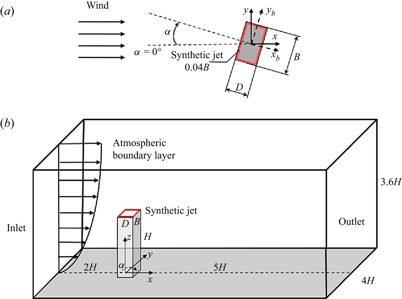
A rigid generic simplified benchmark geometry, known as the CAARC standard tall building model (Melbourne Reference Melbourne1980), has the following dimensions: depth of  $D=30.48$ m, width of
 $B=45.72$ m and height of
 $H=182.88$ m. The computational model used in the present work was a 1/400 scale CAARC building model. The Reynolds number based on the building width is
 ${{Re}_B}={U_H}{B}/{\nu }=24\,000$, where
 ${U_H}$ is the oncoming mean velocity at the height of the building and
 $\nu$ is the kinematic viscosity. From the experimental measurements of Obasaju (Reference Obasaju1992), it can be observed that most of the unsteady loading variation is captured in the
 $0^\circ$ to
 $45^\circ$ range. Thus four different oncoming wind angles with respect to the shorter cross-sectional side of the building (see figure 1a),
 $\alpha =0^\circ$,
 $10^\circ$,
 $20^\circ$ and
 $45^\circ$, were investigated numerically. When at
 $\alpha =0^\circ$, the flow set-up of simulation matched the unforced case of our previous work (Hu & Morgans Reference Hu and Morgans2022).
(a) Top surface of the high-rise building; (b) flow set-up, showing the CAARC building model, ground, the atmospheric boundary layer and the computational domain. The red rectangle denotes the location of the synthetic jet open-loop forcing, which is in the upward ( $z$) direction.

Figure 1(b) shows the sketch of the computational domain used. The origin of the solution domain is defined on the junction of the CAARC building model and the ground, centred on the building axis. The free stream flows in the  $+x$ direction; the horizontal direction normal to the flow and the vertical (building spanwise) direction are designated by the
 $y$-axis and
 $z$-axis, respectively. The size of the domain was chosen according to Architectural Institute of Japan (AIJ) recommendations (Tominaga et al. Reference Tominaga, Mochida, Yoshie, Kataoka, Nozu, Yoshikawa and Shirasawa2008; Tominaga Reference Tominaga2015). The domain cross-section is set to 4
 $H$ (width)
 $\times$ 3.6
 $H$ (height), while the distance between the building axis and the inlet boundary upstream of the building is 2.08
 $H$. The downstream length of the domain is chosen to be approximately 5
 $H$ to ensure that the wake behind the building can fully develop (Tominaga et al. Reference Tominaga, Mochida, Yoshie, Kataoka, Nozu, Yoshikawa and Shirasawa2008). The resulting blockage ratio of the computational domain is 1.6
 $\%$, less than the limitation of 3
 $\%$ suggested by Franke et al. (Reference Franke, Hellsten, Schlunzen and Carissimo2011).
No-slip boundary conditions were applied on the body surfaces and the ground. A free-slip condition was set on the domain sides and a convective outlet condition was set on the domain outlet to avoid backflow. The same inlet boundary condition reported in the study of Hu & Morgans (Reference Hu and Morgans2022) is employed. The ‘target’ mean wind velocity profile was set to the power law (Melbourne Reference Melbourne1980; Huang, Luo & Gu Reference Huang, Luo and Gu2005)  $U = {U_H}({{z}/{H}})^\alpha$, where
 ${U_H}=3$ m s
 $^{-1}$ represents the oncoming velocity at the height of the building and the exponent
 $\alpha$ was chosen to be 0.25. This is a fully developed turbulent boundary layer that can mimic realistically the atmospheric boundary layer. The details of the prescribed atmospheric boundary layer are given in Appendix A. The synthetic eddy method, introduced by Jarrin et al. (Reference Jarrin, Benhamadouche, Laurence and Prosser2006), was used to generate an inflow velocity profile with the ‘target’ mean flow and turbulent characteristics. This method shows a good performance in reproducing the prescribed turbulence characteristics and was well tested and validated in our previous study (Hu & Morgans Reference Hu and Morgans2022).
Flow forcing is provided by a zero-net-mass-flux synthetic jet. The modelling of the actuation is kept simplistic and the jet cavity is not resolved. The slot on the top surface of the building model is designed as the synthetic jet exit, and it is positioned around the perimeter of the top surface with a width of 0.04 $B$, as shown in figure 1. The boundary condition of the actuation is described by a periodic velocity profile. The components of the instantaneous velocity vector at the actuation slot exit are
 $$\begin{gather} {u_{{jet}}} = {v_{{jet}}} = 0, \end{gather}$$
 $$\begin{gather}{w_{{jet}}} = {U_f}\sin (2\pi {f_f}t), \end{gather}$$
where  $u$,
 $v$ and
 $w$ are, respectively, the velocity components along the
 $x,y$ and
 $z$ directions, and
 $U_f$ is the maximum jet velocity. The forcing amplitude ratio
 $A^*$, defined as
 $U_f/U_H$, is chosen as 1 following the optimal suction ratio suggested by Wang et al. (Reference Wang, Peng, Li and He2018). The only variable parameter of the actuation was the forcing frequency. The spanwise vortex shedding frequency for the unforced case at
 $\alpha =0^\circ$ is
 $St_0=0.1$ (Hu & Morgans Reference Hu and Morgans2022), where
 $St=fB/U$ is the Strouhal number based on the building width,
 $B$, and f is the frequency. The forcing frequency,
 $St_f$ is typically non-dimensionalized by the vortex shedding frequency of the unforced flow,
 $St_0$. Motivated by the successful application of the high-frequency open-loop forcing to bluff-body flows in other contexts (Oxlade et al. Reference Oxlade, Morrison, Qubain and Rigas2015; Zhu & Morrison Reference Zhu and Morrison2021), the dimensionless forcing frequency was set at different values of
 $St_f/St_0=5$, 10 and 15.
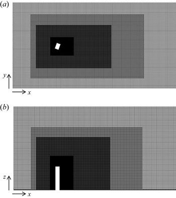
The spatial discretization of the computational domains is performed with an unstructured grid composed of trimmer cells and prism layer cells using StarCCM+. The unstructured grid created and validated in our previous study (Hu & Morgans Reference Hu and Morgans2022) was employed for the case at  $\alpha =0^\circ$. For other wind directions, new grids had to be generated, and the case at
 $\alpha =20^\circ$ is shown as an illustrative example of an inclined building model. Figure 2 shows the grid in the symmetry plane at
 $y=0$ and the
 $xy$ plane at
 $z=0.5H$. The mesh close to the ground and the building is refined to fully resolve the boundary layer using prism layers. In this work, the baseline mesh for the case at
 $\alpha =20^\circ$ was identified via a grid refinement study. Following the experimental measurements (Melbourne Reference Melbourne1980; Obasaju Reference Obasaju1992), the aerodynamic forces in axes fixed on the building body across different wind angles are mainly considered. Defining
 $F_{xb}$ and
 $F_{yb}$ as the aerodynamic pressure forces normal to the rear face and side face of the building model (
 $x_b$-direction and
 $y_b$-direction in figure 1a) respectively, the corresponding non-dimensional aerodynamic force coefficients follow as
 \begin{equation} {C_{Fxb}} = \frac{{{F_{xb}}}}{{0.5\rho U_H^2BH}},\quad {C_{Fyb}} = \frac{{{F_{yb}}}}{{0.5\rho U_H^2BH}}, \end{equation}
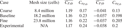
where  $U_H$ is the mean flow velocity at the top of the building. Results from three different grid refinements were compared with the experimental measurement from Obasaju (Reference Obasaju1992), and are summarized in table 1. As compared with the fine mesh, the baseline grid adopts an identical size for the first cell from the building walls, with the wake region relatively less refined. While the coarse mesh under-predicts the fluctuating parts of aerodynamic forces, the differences in values between the baseline and fine mesh suggest that the baseline mesh of 18.2 million cells is sufficiently fine to accurately simulate the flow around the high-rise building.
Baseline grid used for an oncoming wind angle of  $\alpha =20^\circ$: (a)
 $xy$ slice, top view; (b)
 $xz$ slice, side view.

Summary of the grid refinement study for the  $\alpha =20^\circ$ wind angle case. The mean (overbar) and r.m.s. (subscript
 $\sigma$) values of the aerodynamic force coefficients
 $C_{Fxb}$ and
 $C_{Fyb}$ are compared with experimental values from Obasaju (Reference Obasaju1992).

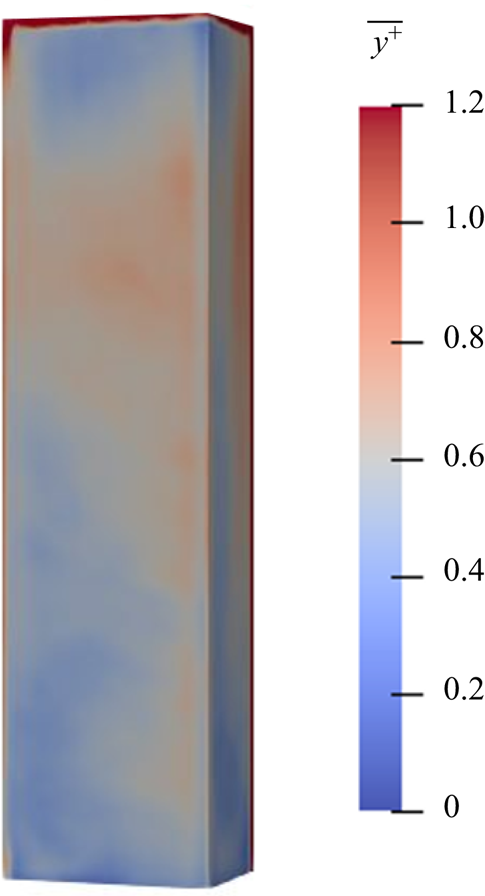
For the baseline mesh for the  $20^\circ$ wind angle, the spatial distribution of
 $y^+$ around the building is shown in figure 3, where it can be observed
 $y^+\simeq 1$. The Courant–Friedrichs–Lewy number in the simulation is dynamic and remains below 0.2. Unsteady simulations were performed on the Imperial College cluster and the ARCHER2 UK computational facility using several hundred cores.
The  $y^+$ colour map on the surface of the building for the baseline mesh at
 $\alpha =20^\circ$.

3. Results and discussion
An active control strategy in the form of a synthetic jet located on the top surface is implemented to attenuate the unsteady loading of the high-rise building across different oncoming wind angles. In this work, the statistics of 32 cycles of the spanwise antisymmetric vortex shedding are sampled for the analysis of the unforced and controlled flows. The aerodynamic characteristics are examined first, after which the time-averaged flow features are investigated. This is followed by the analysis of the effect of the synthetic jet on the unsteady flow features.
3.1. Aerodynamic characteristics
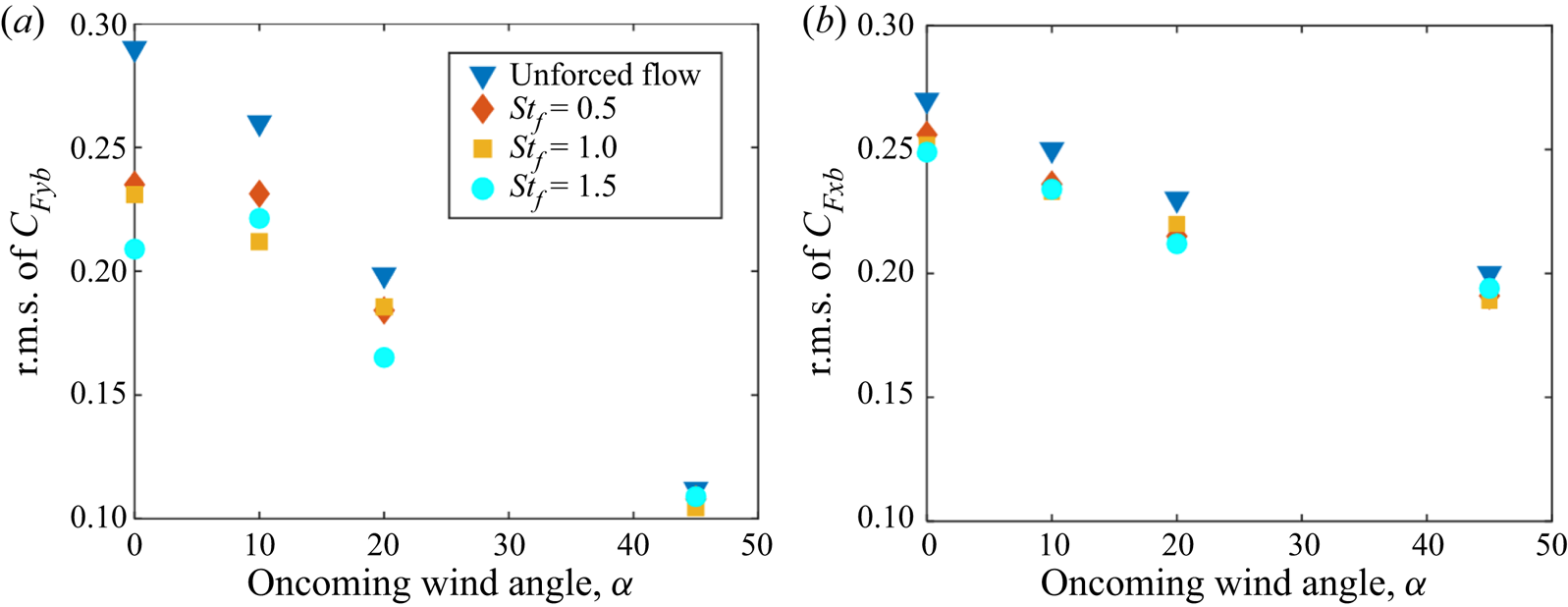
Figure 4 presents the fluctuating aerodynamic coefficients of a high-rise building, the root-mean-square (r.m.s.) values of  $C_{Fyb}$ and
 $C_{Fxb}$, under the influence of a synthetic jet at different angles of attack, where the unforced case serves as a benchmark for comparison.
Variation of fluctuating aerodynamic coefficients for different oncoming wind angles: (a) the r.m.s. value of  $C_{Fyb}$; (b) the r.m.s. value of
 $C_{Fxb}$.

For the unforced case, the fluctuation of the side force,  $C_{Fyb}$, exhibits a maximum value of 0.29 at
 $\alpha =0^\circ$, this value reducing as the oncoming wind angle increases from
 $0^\circ$ to
 $45^\circ$. The r.m.s. values of
 $C_{Fyb}$ are respectively 0.26, 0.20 and 0.11 at
 $\alpha =10^\circ$,
 $20^\circ$ and
 $45^\circ$, matching the experimental measurements from Obasaju (Reference Obasaju1992) well, and further confirming the reliability of the simulations.
In the presence of the top-surface active control, figure 4(a) shows that its effect is to significantly attenuate the fluctuation of  $C_{Fyb}$ for oncoming wind angles of
 $\alpha =0^\circ$,
 $10^\circ$ and
 $20^\circ$. The attenuation remains present but smaller for
 $\alpha =45^\circ$, although the fluctuations are so much smaller in the absence of control at this wind angle. For the wind angles of
 $\alpha =0^\circ$ and
 $20^\circ$, the most effective forcing frequency is
 $St_f=1.5$, for which the r.m.s. values of
 $C_{Fyb}$ are reduced respectively by approximately 25
 $\%$ and 15
 $\%$ compared with the unforced cases. Effective attenuation is also achieved for forcing frequencies of
 $St_f=0.5$ and 1. At
 $\alpha =10^\circ$, while the minimum value of the side-force fluctuation occurs for
 $St_f=1$, control remains almost as effective at the higher forcing frequency of
 $St_f=1.5$, which decreases the r.m.s. value of
 $C_{Fyb}$ by 15
 $\%$.
The fluctuations of  $C_{Fxb}$ across different forcing frequencies are shown in figure 4(b). For the unforced flow, the r.m.s. value of
 $C_{Fxb}$ falls off with increasing wind angle, although this is less pronounced than the
 $C_{Fyb}$ falloff. The effect of open-loop forcing is to reduce these fluctuations for all three forcing frequencies and across all wind angles, although the effect is less pronounced than for
 $C_{Fyb}$. This is consistent with the fluctuating
 $C_{Fxb}$ depending more on the inflow turbulence rather than the near wake dynamics (Obasaju Reference Obasaju1992; Hu & Morgans Reference Hu and Morgans2022). The time-averaged values of
 $C_{Fyb}$ and
 $C_{Fxb}$ have also been checked and found to be mildly reduced by the impact of the synthetic jet.
3.2. Time-averaged flow characteristics
The effect of open-loop control on the time-averaged near wake structures is now investigated. Open-loop forcing at a frequency of  $St_f=1.5$ overall gave the most significant building unsteady loading reductions, with these being most relevant for the smaller wind angles of
 $\alpha =0^\circ$,
 $10^\circ$ and
 $20^\circ$. The effect of the synthetic jet at
 $St_f=1.5$ and across these smaller wind angles is now considered in more detail.
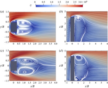
Figure 5(a,c) shows the time-averaged streamlines and streamwise velocity field in the horizontal slice at  $z=0.5H$ at
 $\alpha =0^\circ$ for the unforced and controlled cases, respectively. For the unforced case, the oncoming flow separates at the leading edges of the building, forming bubbles on the side faces of the building. A large low-pressure recirculation region, which is approximately symmetrical about the wake centreline of
 $y=0$, is established behind the building. For open-loop forcing at
 $St_f=1.5$, the size of the recirculation region is extended in the streamwise direction. This is consistent with the attenuation of the spanwise vortex shedding achieved by the synthetic jet, which will be shown later in § 3.3.
Time-averaged streamwise velocity field and projected streamlines for an oncoming wind angle of  $\alpha =0^\circ$. The unforced case: (a) top view in the horizontal plane
 $z=0.5H$, (b) side view in the symmetry plane
 $y=0$. The controlled case of
 $St_f=1.5$: (c) top view in the horizontal plane
 $z=0.5H$, (d) side view in the symmetry plane
 $y=0$.

The time-averaged streamwise velocity field on the  $xz$ plane at
 $y=0$ for the unforced case is shown in figure 5(b). The main flow separates at the leading edge of the top surface, and the downwash free-end shear layer meets with the upwash flow originating from the ground, forming a saddle point at
 $z=2.7B$. For forcing at
 $St_f=1.5$, it can be observed that the separated shear layer is closer to the top surface, and the streamlines in the vicinity of the trailing edge slot are slightly affected by the motion of the synthetic jet. The size of the flow reversal zone in the near wake enlarges, which corresponds to the increase in the recirculation region in the
 $xy$ plane. Moreover, the saddle point is located at
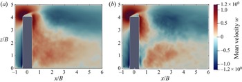
 $z=2.1B$, much lower than the unforced case, illustrating the enhancement of the downwash flow. Figure 6 shows the time-averaged vertical velocity field on the
 $xz$ plane at
 $y=0$ for the unforced and controlled cases. The region with negative
 $w$ is noticeably expanded towards the ground in the vertical direction, consistent with the movement of the saddle point in figure 5 and indicating the downwash flow is strengthened under the impact of the synthetic jet. The enhanced downwash flow also causes downward (rather than upward) flow near the lower part of the back face of the building, which is associated with the formation of the small weak vortex structure near the junction of the building with the ground shown in figure 5(d).
Time-averaged vertical velocity distribution on the  $xz$ plane at
 $y=0$ for an oncoming wind angle of
 $\alpha =0^\circ$. (a) The unforced case, (b) the controlled case of
 $St_f=1.5$.

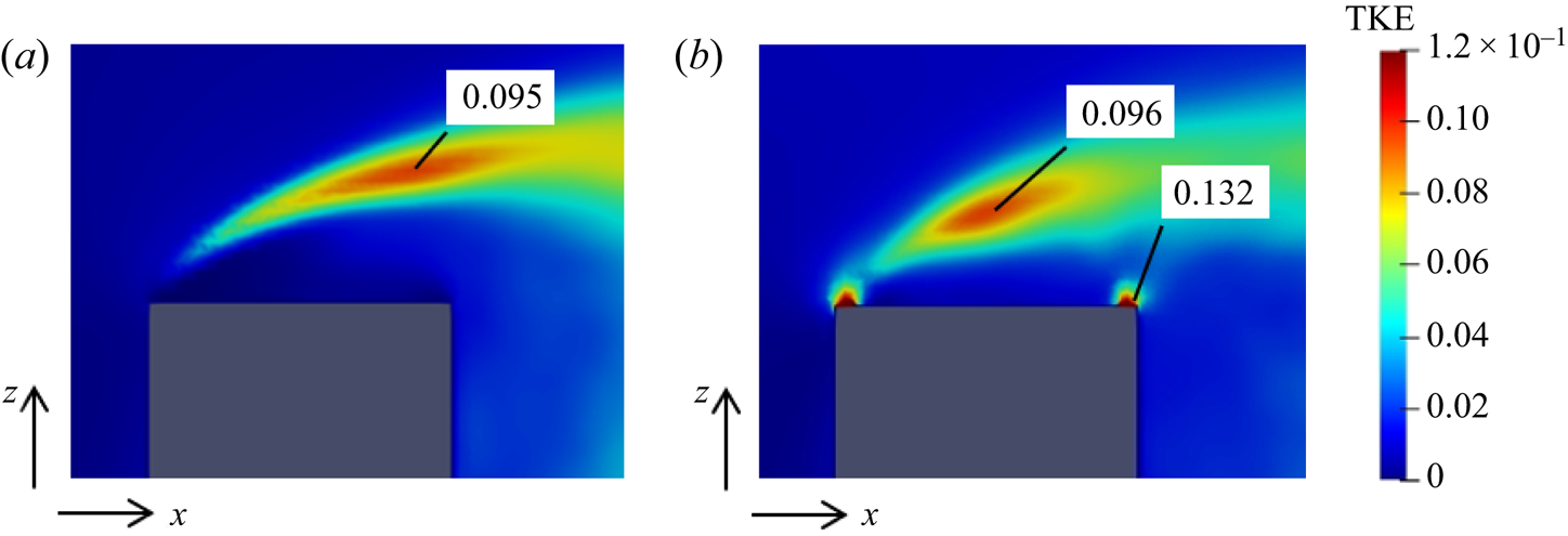
Figure 7 shows the distribution of turbulent kinetic energy (TKE) of the free-end shear flow on the  $xz$ plane, offering insights into the strength of momentum transport in the flow near the top surface (Wang et al. Reference Wang, Peng, Li and He2018). For the unforced case, a large high-value region of TKE associated with the shear layer flow is mainly located above the top surface, and the peak value occurs at
 $z=1.08H$ near the trailing edge of the top surface. For the controlled case, the TKE exhibits a triple-peak distribution, where two peaks are located near the slot exit of the synthetic jet, and the other, associated with the separated flow, occurs further upstream and closer to the top surface compared with the unforced case. The maximum TKE occurring near the slot exit is significantly higher than for the unforced case, and the region with a relatively high TKE value shows a wider vertical spread above the top surface of the building. The synthetic jet strengthens the turbulent fluctuation near the top surface of the building, and Wang et al. (Reference Wang, Peng, Li and He2018, Reference Wang, Zhao, Zeng, Mahbub and Tang2022) suggested that this strong turbulent fluctuation can enhance the momentum transport between the high-momentum main flow and the wake, thus further inducing the stronger downwash flow.
The TKE distribution near the top surface at  $y=0$ for an oncoming wind angle of
 $\alpha =0^\circ$. (a) The unforced case, (b) the controlled case of
 $St_f=1.5$. Local maxima in the TKE are marked as values in the plots.

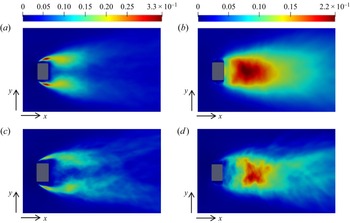
The time-averaged Reynolds stresses on the horizontal slice at  $z=0.5H$ for the unforced case and the controlled case of
 $St_f=1.5$ are compared in figure 8. For the unforced case, the time-averaged streamwise Reynolds normal stress
 $u'u'/U_\infty ^2$ presents a double-peak pattern, which is symmetric about the centreline. The peaks are located in the separated shear layers around the building with a maximum of 0.33. A similar distribution pattern is observed for open-loop forcing at
 $St_f=1.5$, but with the maximum of
 $u'u'/U_\infty ^2$ being significantly reduced to 0.24. The
 $u'u'/U_\infty ^2$ values in the separated shear layer region are also reduced compared with the unforced case.
Time-averaged Reynolds stress distributions in the horizontal slice at  $z=0.5H$ for an oncoming wind angle of
 $\alpha =0^\circ$:
 $u'u'/U_\infty ^2$ and
 $v'v'/U_\infty ^2$ for (a,b) the unforced case; (c,d) the controlled case of
 $St_f=1.5$.

The distribution of  $v'v'/U_\infty ^2$ for the unforced case is shown in figure 8(b). Since the antisymmetric vortices from two side edge shear layers oscillate periodically in the
 $y$-direction, a single-peak distribution of
 $v'v'/U_\infty ^2$ is observed with a maximum of 0.23 occurring along the centreline, with streamwise location
 $x/B=1.59$. In the presence of the synthetic jet at
 $St_f=1.5$, the peak of
 $v'v'/U_\infty ^2$, corresponding to the spanwise vortex, is pushed much further downstream to near
 $x/B=2.09$, with its value reduced by 15.3
 $\%$. This indicates that the synthetic jet successfully pushes the spanwise vortex shedding further downstream and weakens it in the process, which is ascribed to the enhancement of the downwash flow.
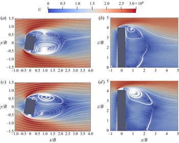
Figure 9 shows the effect of open-loop control on the time-averaged streamlines and velocity field in the horizontal slice for an oncoming wind angle of  $\alpha =10^\circ$. For the unforced case, the main flow also separates at the leading edges, and no reattachment occurs on the side faces. However, the mean wake structures behind the building are not symmetric about the centreline; the vortex structure near the lower side is larger than that close to the upper side. The controlled flow also shows asymmetry in the mean wake topology, but with the recirculation region extending further downstream similar to the effect at
 $\alpha =0^\circ$.
Time-averaged streamwise velocity field and projected streamlines for an oncoming wind angle of  $\alpha =10^\circ$. The unforced case: (a) top view in the horizontal plane
 $z=0.5H$, (b) side view in the symmetry plane
 $y=0$. The controlled case of
 $St_f=1.5$: (c) top view in the horizontal plane
 $z=0.5H$, (d) side view in the symmetry plane
 $y=0$.

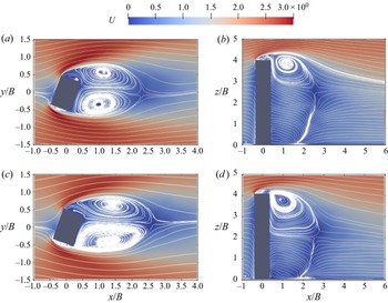
The effect of control at an oncoming wind angle of  $\alpha =20^\circ$ is shown in figure 10. The reattachment of the separated shear layer can be observed on the lower side faces of the building for the unforced case, different to the flows at
 $\alpha =0^\circ$ and
 $10^\circ$. A second flow separation occurs at the trailing edge of the lower side, forming the recirculation region behind the building. The open-loop control has little impact on the reattachment but still extends the size recirculation region in the streamwise direction.
Time-averaged streamwise velocity field and projected streamlines for an oncoming wind angle of  $\alpha =20^\circ$. The unforced case: (a) top view in the horizontal plane
 $z=0.5H$, (b) side view in the symmetry plane
 $y=0$. The controlled case of
 $St_f=1.5$: (c) top view in the horizontal plane
 $z=0.5H$, (d) side view in the symmetry plane
 $y=0$.

The time-averaged velocity fields on the  $xz$ plane at
 $\alpha =10^\circ$ and
 $20^\circ$ are also shown in figures 9 and 10, respectively. The flow patterns of the unforced flow at these two angles do not change much compared with the case at
 $\alpha =0^\circ$. At
 $\alpha =10^\circ$ and
 $20^\circ$, the control extends the flow reversal zone and enhances the downwash flow, similar to its effect at
 $\alpha =0^\circ$.
3.3. Unsteady flow characteristics
In order to better understand the mechanism by which the actuation attenuates the unsteady loading, the unsteadiness in the flow around the building under the effect of the open-loop control is further investigated. The frequency spectra of the fluctuating side force for the unforced and controlled cases are examined first, after which the flow structures caused by the synthetic jet are investigated.
3.3.1. Frequency analysis
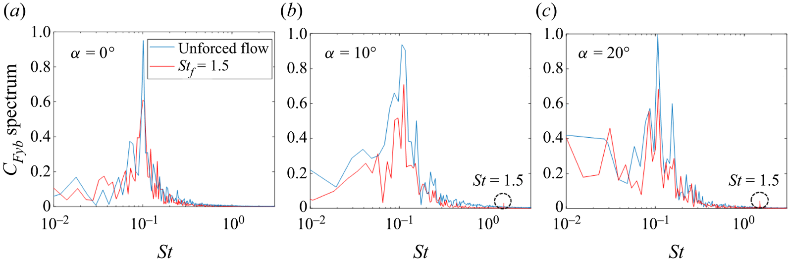
The spectra of the side-force fluctuation are compared for the unforced and controlled cases for three oncoming wind angles in figure 11. For the unforced case, the main spectrum peak in the side-force fluctuation, corresponding to antisymmetric vortex shedding (Hu & Morgans Reference Hu and Morgans2022), occurs at the same frequency  $St=0.1$ for cases of
 $\alpha =0^\circ$,
 $10^\circ$ and
 $20^\circ$. Defining
 $St'$ as the Strouhal number taking the width of the building model normal to the flow as the reference length, these peak frequencies are respectively
 $St'=0.1$, 0.11 and 0.118, showing good agreement with the dominant frequencies reported in the experimental study of Obasaju (Reference Obasaju1992). In the presence of control at
 $St_f=1.5$, the fluctuation of
 $C_{Fyb}$ still exhibits a narrow peak associated with the spanwise vortex shedding at around
 $St=0.1$ for all three wind angles, but these dominant peak values are significantly reduced compared with the unforced case. Thus the synthetic jet is effective in attenuating the side-force fluctuations.
Normalized spectra of the building's side-force fluctuation,  $C_{Fyb}$ at (a)
 $\alpha =0^\circ$; (b)
 $\alpha =10^\circ$; (c)
 $\alpha =20^\circ$.

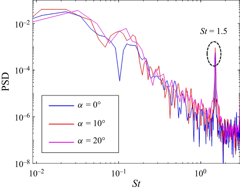
The power spectral densities of  $C_{Fxb}$ are compared in figure 12. The spectra in the presence of control exhibit a peak at the forcing frequency,
 $St=1.5$, indicating the direct influence of the synthetic jet on the separated shear layer flow near the top surface. Interestingly, for the spectra of the side-force fluctuations,
 $C_{Fyb}$, the peak corresponding to the forcing frequency can be also observed at
 $\alpha =10^\circ$,
 $20^\circ$, but not at
 $\alpha =0^\circ$, where
 $C_{Fyb}$ does not include any component in the along-wind direction. This suggests that the synthetic jet does not directly affect the fluctuation of the force in the cross-wind direction, which might lead to the absence of the peak at the forcing frequency for the controlled case at
 $\alpha =0^\circ$.
Power spectral density of  $C_{Fxb}$ of the building in the controlled cases across different oncoming wind angles, where filtering is applied using the pwelch function for clarity.

3.3.2. Jet behaviour
The synthetic jet on the top surface successfully attenuates the side-force fluctuation of a high-rise building, and thus it is of interest to analyse the unsteady flow structures generated by the synthetic jet. In this section, the immediate flow field in the vicinity of the synthetic jet is characterized for the control case of  $St_f=1.5$ at
 $\alpha =0^\circ$.
The velocity forcing direction of the synthetic jet positioned on the top surface is coincident with the  $z$-axis, as shown in figure 1. The flow around the building under the effect of the synthetic jet is complex, highly turbulent and comprises both large-scale structures and fine-scale turbulent fluctuations. Since our main interest is the former, modal decomposition was applied to the unsteady flow field. Spectral proper orthogonal decomposition (SPOD) proposed by Towne, Schmidt & Colonius (Reference Towne, Schmidt and Colonius2018), an empirical method to identify spatial-temporal coherent structures, was performed based on the time-resolved flow data. Compared with the space-only proper orthogonal decomposition, SPOD is able to extract coherent structures oscillating at a certain frequency (Schmidt et al. Reference Schmidt, Towne, Rigas, Colonius and Brès2018; Towne et al. Reference Towne, Schmidt and Colonius2018), which enables analysis of the dominant structures associated with the synthetic jet at its forcing frequency.
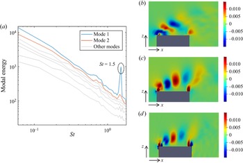
The SPOD was performed based on the streamwise and vertical velocity fluctuations on the  $xz$ plane for the region close to the top surface, as shown in figure 13(b–d). A total of 650 snapshots with a sampling time step of 0.01 s were collected, and 9 blocks with 50
 $\%$ overlap were generated for the discrete Fourier transform analysis in the decomposition. The Hamming window function was applied to each block in order to avoid spectral leakage. The SPOD modal energy spectrum for the fluctuating kinetic energy of the plane at
 $y=0$ is shown in figure 13(a), with a peak at the forcing frequency
 $St=1.5$ present in mode 1, which contains the most energy and thus plays a dominant role.
The SPOD spectra and first SPOD mode on the  $xz$ plane at
 $y=0$ for the controlled case at
 $\alpha =0^\circ$: (a) SPOD energy spectra; (b) streamwise velocity component of the first SPOD mode at
 $St=1.5$; (c) vertical velocity component of the first SPOD mode at
 $St=1.5$; (d) first SPOD mode of
 $\omega _y$ at
 $St=1.5$.

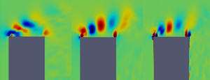
Figure 13(b,c) shows respectively the streamwise and vertical velocity components of the first SPOD mode at  $St=1.5$. The strong oscillation in these two velocity components is observed above the top surface of the building, suggesting that coherent structures occur here. The first SPOD mode of the corresponding vorticity,
 $\omega _y$, at the forcing frequency is further visualized in figure 13(d). Small vortex structures near the slot exits on the leading and trailing edges are observed. The height of these coherent structures increases gradually from the leading edge to the trailing edge, which can be ascribed to the separated shear flow near the top surface. The coherent vortex structures caused by the synthetic jet significantly enhance the turbulent fluctuations above the top surface as well as the momentum transport, consistent with the TKE results observed in figure 7. Wang et al. (Reference Wang, Peng, Li and He2018, Reference Wang, Zhao, Zeng, Mahbub and Tang2022) suggested that this enhanced momentum transport can further induce a stronger downwash flow.
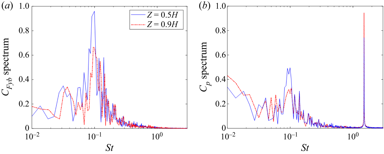
To understand further the effect of the synthetic jet, the fluctuation of the side-face pressure force was investigated for the controlled case. The normalized spectra of the side-force coefficient,  $C_{Fyb}$, at different heights for the controlled case of
 $St_f=1.5$ are shown in figure 14, where the peaks at the forcing frequency are not observed. However, since the slot of the synthetic jet is positioned around the top surface, as shown in figure 1, the flow from the slot exits near the two side edges inevitably affects the pressure of the building's side faces. Figure 14 shows the spectra of the pressure coefficient only on one side face,
 $C_p$, for the controlled flow. It is observed that a narrow peak in
 $C_p$ occurs near the forcing frequency,
 $St_f=1.5$, indicating flow structures directly caused by the actuation exist near the two side faces. These flow structures are likely to be symmetric about the wake centreline, accounting for the observation that no spectral peak in
 $C_{Fyb}$ occurs at the forcing frequency.
(a) Normalized spectra of  $C_{Fyb}$ at different heights of the CAARC building. (b) Normalized spectra of
 $C_p$ at different heights.

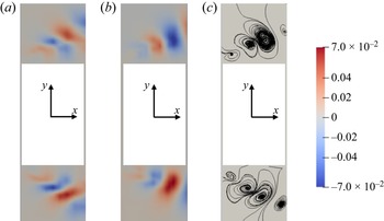
The streamwise and vertical velocity components of the first SPOD mode at the forcing frequency in the  $xy$ plane at
 $z=0.9H$ are shown in figure 15, and are seen to exhibit symmetric coherent structures. Figure 15(c) shows the streamlines denoting the real-part mode shape of the vector composed of these two velocity components. The vortex structures formed near two sides of the building are completely symmetric about the wake centreline, illustrating the synthetic jet on the top surface has no direct impact on the net side-force fluctuation. The symmetric coherent structures are ascribed to the flow from the jet exit close to two side edges.
First SPOD mode around the building on the horizontal slice at  $z=0.9H$ for the controlled case at
 $\alpha =0^\circ$. (a) Streamwise velocity component of the first SPOD mode at
 $St=1.5$; (b) vertical velocity component of the first SPOD mode at
 $St=1.5$; (c) generated streamlines.

3.3.3. Near wake structures
The unsteady wake flow around the building determines the building's unsteady loading. As already discussed, the action of the open-loop forcing, the synthetic jet on the top surface, is to enhance the downwash flow, subsequently affecting the wake. The corresponding effect of this forcing on the near wake structures around the building is now analysed.
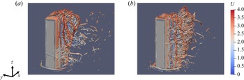
Snapshots of the instantaneous flow fields around the high-rise building for the unforced case and the controlled case are illustrated in figure 16, where the vortical structures are identified by the iso-surfaces of the Q-criterion. The horseshoe vortex wrapping around the front bottom of the building can be observed in both cases, while the shear layer flow separated from the top-surface leading edge is much closer to the building top surface in the presence of control, consistent with the time-averaged results obtained in § 3.2. Moreover, the vortices in the wake behind the building are shifted to the lower positions under the effect of the synthetic jet, consistent with the enhancement of the downwash flow.
Instantaneous snapshots for iso-surfaces of Q-criterion coloured by velocity at  $\alpha =0^\circ$ in (a) the unforced case; (b) the controlled case of
 $St_f=1.5$.

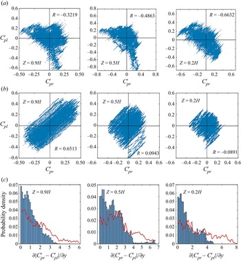
For the unforced case, two types of spanwise vortex shedding behaviour, antisymmetric and symmetric vortex shedding, have been identified in the flow around the building immersed in the atmospheric boundary layer. The antisymmetric vortex shedding mode is prevalent in the near wake and dominates the unsteady loading on the building (Hu & Morgans Reference Hu and Morgans2022). The effect of the synthetic jet on the spanwise vortex shedding is now investigated in more detail. Figure 17 shows the fluctuations of the pressure coefficient on the right and left side faces of the building,  $C_{pr}'$ and
 $C_{pl}'$, for the unforced flow and in presence of control at three different heights of the building. The instantaneous results of 40 000 samples are shown in these scatter plots. These plots are able to shed light on the side-to-side symmetry of the fluctuations (Bourgeois, Noack & Martinuzzi Reference Bourgeois, Noack and Martinuzzi2013). If the fluctuations are in phase, corresponding to symmetric flow structures, a positive gradient will be observed, while if the fluctuations are out of phase, corresponding to antisymmetric fluctuations, a negative gradient will dominate.
Scatter plot for the fluctuation of the pressure coefficient on the right and left building side faces for a wind angle of  $\alpha =0^\circ$ for (a) the unforced case and (b) the controlled case of
 $St_f=1.5$. (c) The corresponding probability distribution of the side pressure gradients for the uncontrolled case (red lines) and the controlled case (blue bars). Three different heights are considered,
 $z=0.9H$ near the building top,
 $z=0.5H$ at the half-height position and
 $z=0.2H$ near the base.

For the unforced case at  $z=0.9H$, the pressure fluctuations on the two opposing faces are negatively correlated, with a correlation coefficient of
 $-$0.3219. However, at the same height but in the presence of control at
 $St_f=1.5$, most scatter points are located in the first and third quadrants, with the correlation coefficient between
 $C_{pl}'$ and
 $C_{pr}'$ being 0.6513. The pressure fluctuations on opposing side faces are in phase most of the time, indicating that the antisymmetric vortex shedding gets significantly suppressed. At
 $z= 0.5H$, the correlation coefficients between
 $C_{pl}'$ and
 $C_{pr}'$ are
 $-$0.4863 for the unforced flow and 0.0943 with control, while at
 $z = 0.2H$ they are
 $-$0.6632 and
 $-$0.0891, respectively. Moreover, the effect of the synthetic jet on the side pressure gradient probability density is also shown in figure 17. In the presence of control, the side pressure gradient exhibits a distribution much more concentrated around 0 at all three different heights of the building, which also indicates the weakened antisymmetric vortex shedding.
All of these indicate that the synthetic jet weakens the antisymmetric vortex shedding behaviour and enhances the symmetric vortex shedding behaviour along the entire height of the building by enhancing the downwash flow. Since the effect of enhanced downwash flow gradually retreats close to the ground, spanwise antisymmetric vortex shedding is most significantly weakened near the building top. These observations are consistent with the findings reported by Wang & Zhou (Reference Wang and Zhou2009), Behera & Saha (Reference Behera and Saha2019) and da Silva et al. (Reference da Silva, Chakravarty, Sumner and Bergstrom2020) that the free-end downwash flow postpones the antisymmetric vortex shedding.
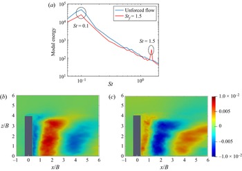
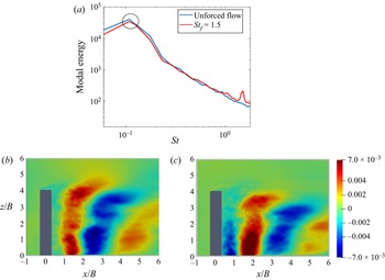
In order to further investigate the effect of the synthetic jet on spanwise vortex structures, modal decomposition was also applied to the wake, with SPOD used for wake structure visualization. Figure 18(a) shows the energy spectra of the first mode from SPOD of the cross-wise velocity component on the  $xz$ plane at
 $y=0.44B$ for the unforced and controlled cases. For both cases, the spanwise vortex shedding frequency,
 $St=0.1$, contains the most energy, as indicated by the main peaks. For the controlled case, the second peak occurs at
 $St=1.5$ corresponding to the forcing frequency. Figure 18(b,c) shows the first SPOD mode of the cross-wise velocity component at the spanwise vortex shedding frequency,
 $St=0.1$, for the unforced case and the controlled case, respectively. The first mode for these two cases exhibits similar behaviours: coherent structures corresponding to antisymmetric vortex shedding are observed, with the structures shed uniformly along the entire building height. However, in the presence of the synthetic jet, the dominant coherent structures are weakened and appear further downstream. This is consistent with the attenuation of the pressure force fluctuations occurring in the presence of control.
The SPOD spectra and first SPOD mode on the  $xz$ plane at
 $y=0.44B$ for an oncoming wind angle of
 $\alpha =0^\circ$. (a) Energy spectra of the first SPOD mode for the unforced case and the controlled case. (b) First SPOD mode of cross-wise velocity component at
 $St=0.1$ for the unforced case. (c) First SPOD mode of cross-wise velocity component at
 $St=0.1$ for the controlled case.

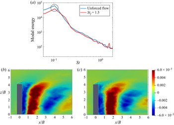
In order to further investigate the effect of the synthetic jet on spanwise vortex structures at  $\alpha =10^\circ$ and
 $20^\circ$, modal decomposition was also applied to the wake, with SPOD used for wake structure visualization. The first SPOD modes of the cross-wise velocity component on the
 $xz$ plane at the spanwise vortex shedding frequency for the cases of
 $\alpha =10^\circ$ and
 $20^\circ$ are shown in figures 19 and 20, respectively. The first modes of the unforced flow at these two wind angles do not change much compared with the case at
 $\alpha =0^\circ$, exhibiting coherent structures along the entire building height corresponding to antisymmetric vortex shedding. For the controlled cases of
 $St_f=1.5$ at
 $\alpha =10^\circ$ and
 $20^\circ$, the actuation slightly weakens the vortex shedding and results in the coherent structures corresponding to it being located further downstream, this being more apparent closer to the ground.
The SPOD spectra and first SPOD mode on the  $xz$ plane at
 $y=0.44B$ for an oncoming wind angle of
 $\alpha =10^\circ$. (a) Energy spectra of the first SPOD mode for the unforced case and the controlled case. (b) First SPOD mode of cross-wise velocity component at
 $St=0.1$ for the unforced case. (c) First SPOD mode of cross-wise velocity component at
 $St=0.1$ for the controlled case.

The SPOD spectra and first SPOD mode on the  $xz$ plane at
 $y=0.44B$ for an oncoming wind angle of
 $\alpha =20^\circ$. (a) Energy spectra of the first SPOD mode for the unforced case and the controlled case. (b) First SPOD mode of cross-wise velocity component at
 $St=0.1$ for the unforced case. (c) First SPOD mode of cross-wise velocity component at
 $St=0.1$ for the controlled case.

4. Conclusion
In this work, an open-loop active control method employing a synthetic jet on the top surface was proposed to mitigate the unsteady loading of a high-rise building exposed to differing oncoming wind directions. A canonical high-rise building, known as the CAARC model, was studied, and four different oncoming wind angles were considered. The behaviour of the synthetic jet and its effect on the flow structures around the building was studied numerically using wall-resolved large eddy simulations.
Synthetic jet open-loop forcing at three different frequencies, all at least half an order of magnitude larger than the main vortex shedding frequency, were considered. Across all conditions, the synthetic jet attenuated the side-force fluctuations of the building. Actuation at the high frequency,  $St_f=1.5$, was identified as exhibiting good performance for all oncoming wind angles. The influence of the synthetic jet on the time-averaged flow structures was analysed, with it being found that the downwash flow is enhanced significantly and the recirculation region is extended in the streamwise direction under its effect.
The effect of control on the frequency spectra of the fluctuating aerodynamic force was investigated, with control seen to weaken the peak at the vortex shedding frequency. A SPOD analysis for the controlled case of  $St_f=1.5$ at an oncoming wind angle of
 $\alpha =0^\circ$ confirmed that the synthetic jet enhances the turbulent fluctuation above the top surface, but has no direct impact on the side-force fluctuation. The enhanced turbulent fluctuation induces a stronger downwash flow, which could further influence the spanwise vortex shedding. The unsteady near wake structures in the unforced and controlled cases were also investigated, with the synthetic jet found to suppress antisymmetric spanwise vortex shedding and promote symmetric vortex shedding, which is ascribed to the enhanced downwash flow. The formation of dominant vortices is also delayed by the synthetic jet, which can further reduce the pressure fluctuations on the building caused by these vortices. This work provides insights into the control mechanism of how the synthetic jet attenuates the side-force fluctuation of the building at different oncoming wind angles, laying a theoretical basis for the practical application of active control approaches.
Acknowledgements
Both the Imperial College High Performance Computing facilities and ARCHER2 (the UK National Supercomputing service) used in this work are acknowledged. The authors greatly acknowledge the President's PhD Scholarship from Imperial College London for funding this research.
Funding
This research was supported by the Imperial College President's PhD Scholarship scheme.
Declaration of interests
The authors report no conflict of interest.
Appendix A. Turbulent inflow
The same turbulent inlet boundary condition reported in the study of Hu & Morgans (Reference Hu and Morgans2022) is employed. The ‘target’ features were characterized using the turbulence intensity profile, following AIJ standards (Tominaga et al. Reference Tominaga, Mochida, Yoshie, Kataoka, Nozu, Yoshikawa and Shirasawa2008) and experimental data from Obasaju (Reference Obasaju1992), Ngooi (Reference Ngooi2018) and Huang et al. (Reference Huang, Luo and Gu2005). This profile is shown below, where  $I(z)$ is the streamwise turbulence intensity at height
 $z$ and
 $I_H$ is the streamwise turbulence intensity at the height of the building
 \begin{equation} I(z) = {I_H}{\left( {\frac{z}{H}} \right)^{ - \alpha - 0.05}}. \end{equation}
Here,  $I_H$ was set to 13
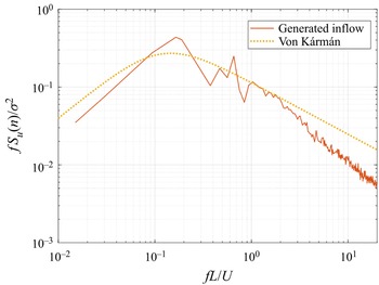
 $\%$. The power spectral density (PSD) of velocity in a realistic atmospheric boundary layer should satisfy the von Kármán spectrum. The normalized PSD of streamwise velocity at the building height for the generated turbulence is compared with the target von Kármán spectrum in figure 21, showing that the fluctuating velocity satisfies the spectral model for accurate predictions of wind effects on the building.
Comparison of PSD in the flow direction with the von Kármán spectrum at the model building height.