1. Introduction

Gabriel Dover once complained that being nearly neutral is like being “just a little bit pregnant” (Dover Reference Dover1997, 91). Dover's point is that “nearly neutral” really means “a little bit selective,” and once you’ve allowed for a little bit of selection, what's to stop more and more selection from being incorporated into your model?Footnote ¹ And then, does anything remain of neutrality? Dover's comment thus calls into question the role of both selection and drift in the nearly neutral theory.

The neutral theory was articulated and defended by Motoo Kimura as a way to explain molecular variation and evolution. From its introduction in 1968, the neutral theory posited that evolution at the molecular level did not proceed by selection alone. The nearly neutral theory of molecular evolution was introduced in 1973 by Tomoko Ohta as a variant of the neutral theory. Ohta worked closely with Motoo Kimura and like Kimura was especially interested in explaining molecular evolution with a combination of drift and selection.

In this article we will use Millstein's (Reference Millstein2002, Reference Millstein2005) distinction between process and outcome to distinguish the roles of drift and selection in both the neutral and nearly neutral theories. We will defend the claim that, as a conceptual matter, the neutral and nearly neutral theories are not only about drift—both drift and selection understood as processes figure importantly in both theories. As theories of the combined action of drift and selection, advocates of the neutral theory and the nearly neutral theory are particularly attuned to the problem of distinguishing drift from selection. We interpret their success in empirically differentiating drift and selection in terms of ongoing efforts to find unique ways to detect causal processes by articulating determinative associations between outcomes and processes.

2. Process and Outcome in Molecular Evolution

By “causal process” we mean a series of causally connected physical states occurring over time, whereas by “outcome” we mean the effect, or ending state at a particular point in time, of that process (or any series of such ending states).Footnote ² In order to understand why the distinction between process and outcome is important for distinguishing drift from selection, consider Kimura's definition of drift: “By random genetic drift I mean random fluctuation of gene frequencies in a population caused by random sampling of gametes in reproduction. In any sexually reproducing species, the total number of individuals is not only finite, but also can be regarded as a random sample chosen from a much larger collection of male and female gametes (or ‘gene pool’) produced by the parental generation. The amount of fluctuation in gene frequencies (that is, proportion of various alleles) is expected to be larger, the smaller the population” (Kimura Reference Kimura1983, 37). Notice that Kimura's definition of drift incorporates both “process” and “outcome”; the “process” is the random sampling of gametes, and the “outcome” is the random fluctuation of gene frequencies. This definition creates an ambiguity, an ambiguity that is not unique to Kimura: are all instances of random sampling instances of drift? Are all random fluctuations in gene frequencies instances of drift? The latter was suggested by Wright (Reference Wright1955), but it is problematic to define drift in this way. The same type of outcome, where gene frequencies appear to fluctuate randomly from one generation to the next, can be produced by selection in a changing environment. Selection in a changing environment is a much different phenomenon than the random sampling of gametes. Thus, however we are to define drift and selection, it cannot be in terms of their outcomes, or we risk being unable to distinguish two very different biological phenomena. Our concepts should be rich enough to capture important biological differences.

A better way of defining drift and selection is in terms of causal processes. As we just noted, Kimura saw the underlying process of drift as random gamete sampling; other biologists have included other types of random sampling such as that occurring when a small subset of founders establish a new population. “Random” sampling is “indiscriminate sampling” (Beatty Reference Beatty1984); in other words, a process in which heritable physical differences between organisms (at any stage, including the gametic) are causally irrelevant to differences in reproductive success (Millstein Reference Millstein2002). Then, selection can be defined in a parallel way, as “discriminate sampling” (Beatty Reference Beatty1984); that is, it can be defined as a process in which physical differences are causally relevant to differences in reproductive success (Millstein Reference Millstein2002). In this way, the concepts distinguish between two biologically important phenomena. We will show that distinguishing the processes of natural selection and random drift and the outcomes of natural selection and random drift is crucial for understanding the neutral and nearly neutral theories conceptually and empirically.

3. The Neutral Theory of Molecular Evolution

When Kimura and others began to champion the neutral theory in the late 1960s and early 1970s, they argued that a significant portion of the observed variations at the molecular level (in proteins and nucleic acids) were neutral or effectively neutral and so subject to drift (King and Jukes Reference King and Jukes1969). Advocating a strong role for neutrality and drift was especially controversial given the strong panselectionist attitude held by most organismal evolutionary biologists at the time (Kimura Reference Kimura1983; Dietrich Reference Dietrich1994, Reference Dietrich1998; Mitchell and Dietrich Reference Mitchell and Dietrich2006). The neutral theory is much more than just a theory of genetic drift, however; selection also plays an important role in the neutral theory.

An important key to understanding the claims made for the neutral and nearly neutral theory lies in the distinction between mutation and substitutions, or, as John Gillespie (Reference Gillespie1991) calls them, origination processes and fixation (substitution) processes. Origination processes account for the origin of mutations. Substitution processes account for what happens to mutants once they are created. Drift and selection are both substitution processes. Kimura, Ohta, and other neutralists freely accepted that many mutations are created that are never detected because most mutants are probably selected against and occasionally a rare advantageous mutation is selected for. These mutants leave the population quickly or go to fixation quickly and so are not detected as differences. Kimura and Ohta would like to explain the observed frequencies of detected variation or polymorphisms. Where leading selectionists argued that detected polymorphisms were actively maintained in a population by selection (balancing selection for heterozygote superior combinations, for instance; Lewontin Reference Lewontin1974), neutralists explained polymorphism in a population as neutral or nearly neutral mutants that were on their way to fixation or loss. These mutants were transient polymorphisms and were detectable simply because they were not quickly eliminated or fixed (Kimura and Ohta Reference Kimura and Ohta1971). The core of the neutralist-selectionist debate then is not an all-or-nothing dispute pitting selection against drift but a debate over the relative importance of drift and selection for explaining these detected polymorphisms in a population.

From the start, Kimura and Ohta recognized that not all neutral mutants were the same. Some mutants were considered to be strictly neutral, whereas others were considered to be nearly (or effectively) neutral. However, once again, there is ambiguity in the definitions. For example, Kimura once described the difference between neutral and nearly neutral mutations as follows: neutral mutations are the result of nucleotide substitutions that yield the same amino acid (“synonymous” mutations),Footnote ³ whereas nearly neutral mutations are those amino acid substitutions where there is “very little effect on the biological activity of the protein” (Kimura Reference Kimura1968b, 247). These definitions are what we might call functional definitions; they focus on the way the protein resulting from the mutation functions in the organism.Footnote ⁴ That is, neutral mutations are considered to be mutations where the same function obtains, whereas nearly neutral mutations are mutations where “nearly” the same function obtains.

Elsewhere, however, Kimura describes the difference between neutral and nearly neutral mutations differently. These definitions seem to focus instead on the expected outcomes of the differing functional types, usually statistical measures of population features such as heterozygosity. Here, neutral mutations are those where the selective coefficient is zero, whereas nearly neutral mutations are those where the selection coefficient is very much less than the inverse of the population size (Kimura Reference Kimura1968a). That is, with nearly neutral mutations, the effects of drift are expected to swamp the effects of weak selection given the population size, that is, they are “effectively” neutral. In contrast, note that the functional definitions are independent of population size. The functional definitions represent a causal approach, rather than an outcome-oriented definition.

We argue that the functional definition of nearly neutral, with its focus on the causal, is preferable to the expected outcome definition. An outcome-oriented approach is essentially claiming that effectively neutral mutations are expected to undergo drift, after which we determine if in fact they have undergone drift.Footnote ⁵ Although this is not, strictly speaking, circular reasoning, it certainly borders on the circular. The causal approach, however, claims that mutations that result in differing functions are expected to undergo weak selection as well as drift. This is less circular; as discussed below, the functional claim can be tested independently of the outcomes for the population.Footnote ⁶

Furthermore, finding an outcome that accurately picks out the drift process and allows it to be distinguished from mixed drift and selection processes and selection processes is not that simple. One of the advantages claimed for the neutral theory when it was initially advocated was that it made quantitative predictions that could be easily tested (Crow Reference Crow1969; Kimura and Ohta Reference Kimura and Ohta1971). So if you thought that neutral mutants were nonsense, you’d be able to demonstrate it quickly and move on to your selectionist program. Unfortunately, drift and selection were not easily distinguished despite the neutral theory's predictions. Important early tests of neutrality and selection did not have enough statistical power (Ewens Reference Ewens1972). Other tests depended on problematic assumptions. The result was that there was not a clear outcome that could unequivocally be said to only result from a process of genetic drift. Put another way, the causal processes associated with selection were acknowledged to be important, but their extent could not be established because the kinds of outcomes presented in the existing molecular data did not allow processes of drift and selection to be clearly distinguished.

All of the early empirical tests of the neutral theory depended on data regarding proteins (either protein sequences, immunological affinities, or electrophoretic analysis). In the mid-1980s, Martin Kreitman introduced DNA sequence analysis into evolutionary genetics. With the rising availability of DNA sequence data thanks to PCR technology, biologists devised much more definitive statistical tests of neutrality and selection. DNA-based tests of neutrality took advantage of phenomena such as the redundancy of the genetic code. Redundancy at the third position of many codons means that nucleotide substitutions will not result in amino acid substitutions at the protein level. These synonymous mutants then should not be subject to selection based on their effect or lack thereof at the protein level.Footnote ⁷ Comparing synonymous and nonsynonymous changes within and between species thus becomes a means of evaluating the relative effects of drift and selection on the sequence in question (Kreitman Reference Kreitman1996, Reference Kreitman2000).

4. The Nearly Neutral Theory

In 1972, Tomoko Ohta began to argue for a more significant role for weakly selected mutants. Ohta's proposal refined the neutral theory by arguing that the large numbers of rare alleles being detected by electrophoretic surveys of natural populations could be explained by positing larger numbers of slightly deleterious mutants (Ohta Reference Ohta1973; Ohta and Gillespie Reference Ohta and Gillespie1996). Ohta's theory was called the nearly neutral theory because it emphasized mutants at the border of neutrality and selection.

According to Ohta and Gillespie (Reference Ohta and Gillespie1996), in the earliest versions of the nearly neutral theory Ohta redefined “nearly neutral” mutants to be those mutants whose selection coefficients are close to the reciprocal of the population size, unlike Kimura's definition of “nearly neutral” (effectively neutral) mutants, where the selection coefficient is much less than the reciprocal of the population size. In making this change, she modified what we have called the “expected outcome” definition of “nearly neutral.” We might also construe various “functional definitions” equivalent to this modified concept of “nearly neutral”; Ohta notes that “the effect of an amino acid substitution in a protein often produces only a minor modification of a reaction coefficient” and that “molecular variants that disturb very slightly the secondary structure of molecules, e.g. by opening the stem region of a clover structure of tRNA, may represent a mutant class with mild deleterious effects” (Ohta Reference Ohta1992, 272).

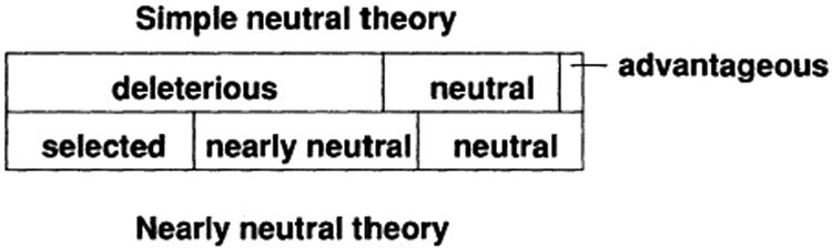
To put the point roughly, Ohta's definition of “nearly neutral” includes mutants that are less neutral than Kimura's “nearly neutral” mutants.Footnote ⁸ Thus, in effect, Ohta introduced a new way of classifying mutants by expanding the category of mutants at the borderline between deleterious and neutral (see Figure 1). The point is to consider specifically which outcomes we should expect if a large proportion of mutations are nearly neutral, rather than strictly or “effectively” neutral.Footnote ⁹

Figure 1.

Distinguishing the neutral and nearly neutral theories. Ohta's “schematic diagram” representing the “proportions of various classes of mutants” (from Ohta Reference Ohta1992, 271).

As we will argue below, formalizing and redefining nearly neutral mutants gave a stronger role to evolution where processes of drift and selection both played significant roles. While the early nearly neutral theory agreed with the strictly neutral or “simple neutral theory” that selected mutants could be advantageous or deleterious, she emphasized that most selected mutants, including nearly neutral mutants, were in fact deleterious to some degree. The chief difference was the expansion of the proportion of nearly neutral mutants.

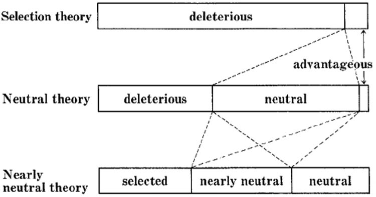
Ohta later refined the nearly neutral theory to include both slightly deleterious and slightly advantageous mutants. She represented this in a diagram from 2002 that shows the successive expansion of what were previously understood to the borders between types of mutants (see Figure 2). So the border between advantageous and harmful selected mutants becomes expanded to include neutral mutants, and the new borders with neutrality each get expanded to create a class of nearly neutral mutants that includes slightly deleterious and slightly advantageous mutants. Ohta lumps advantageous and deleterious mutants together as selected. This allows her to emphasize that the nearly neutral class is intermediate between the selected and neutral classes.

Figure 2.

Ohta's refinement of her schematic diagram for different classes of mutations (from Ohta Reference Ohta2002, 16136).

There is yet another ambiguity here, having to do with whether drift alone is acting on the mutations or drift in combination with selection. The case of strictly neutral mutations is clear-cut; they are subject to drift alone. One could also, if one defines drift by the type of outcome it produces, interpret nearly neutral mutants as being subject to drift alone, since they seem to behave as strictly neutral mutants would. This is what Kimura seems to have done in the 1960s (Kimura Reference Kimura1968a, Reference Kimura1968b) and even in his later writings, where he states that the presence of “nearly neutral but very slightly deleterious” mutations “allows extensive random drift” (Kimura Reference Kimura1983, 143), without any mention of selection.Footnote ¹⁰ On the other hand, if one defines selection and drift in terms of causal processes, as we argued for above, then nearly neutral mutations are subject to very weak selection (discriminate sampling) and to drift in the form of indiscriminate gamete sampling. On the process-oriented view, the effects of drift “swamp” the effects of weak selection for nearly neutral mutations, but both processes are occurring.Footnote ¹¹ We think that this provides a much clearer conceptual picture of the biological phenomena at work.

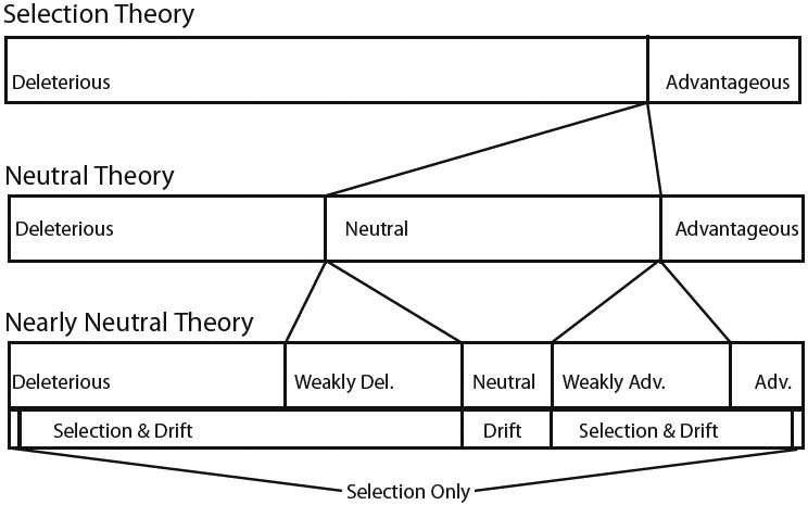
In Figure 3, we have tried to clarify Ohta's schematic diagrams by differentiating between deleterious and advantageous mutations. However, instead of contrasting selected and neutral or nearly neutral mutants, we contrast deleterious, weakly deleterious, neutral, weakly advantageous, and advantageous mutants.Footnote ¹² Ohta's nearly neutral mutants are those that are weakly deleterious or weakly advantageous, where “weakness” is defined in terms of having a selection coefficient less than the reciprocal of the population size. It is important to note that the relative proportions of these different classes of mutants can shift over time, although most biologists would agree that the proportion of advantageous mutants is usually very small and the proportion of deleterious mutations is large. Superimposed on the proportions of mutations are the actions of drift and selection. Following Ohta, neutral mutants are assumed to be strictly neutral and so subject only to drift. A small fraction of mutants at either end of the diagram are also assumed to be so strongly selected that they can be considered to be subject to selection only—these might be lethal mutations, for instance. Most mutations, however, are subject to both selection and drift. In the cases of weak selection, the effects of drift are more prominent, and the resulting outcome is that expected from the nearly neutral theory.

Figure 3.

A revised representation of the nearly neutral theory in relation to selection theory and the neutral theory.

Ohta believed that the mixed processes of drift and selection affecting nearly neutral mutants could be distinguished from drift outcomes associated with strict neutrality. The challenge was to find a way to distinguish them empirically from outcomes associated with stronger selection processes. When Ohta introduced her nearly neutral theory, Kimura's neutral theory was challenged by data on genetic variability measured in population of Drosophila by Francisco Ayala and his coworkers. Ayala's data revealed a large number of relatively rare alleles. This did not conform to the distribution predicted by the neutral theory. Ohta realized that the presence of slightly deleterious alleles could explain this distribution. Ayala's distribution thus became an outcome associated with near neutrality. Ohta later argued that some features of the molecular clock, including its overdispersion, could be best explained by the nearly neutral theory (Ohta Reference Ohta2002). Much of the debate over these nearly neutral explanations has been about whether the nearly neutral theory presents the only route to these outcomes.Footnote ¹³ Martin Kreitman, for instance, points out that while weak selection provides the best explanation of high levels of codon bias, the nearly neutral model is much more difficult to reject on empirical grounds than the neutral model. Selection tests based on ratios of replacement to synonymous changes can easily reject strictly neutral models, thereby making them a good null hypotheses. However, Kreitman argues that the nearly neutral theory is much more difficult to falsify, because it can be rendered consistent with almost any pattern of variation by invoking different histories of changes of population size (Kreitman Reference Kreitman1996, 683). So, while there are some outcomes uniquely associated with the nearly neutral theory, they are not as plentiful or as clearly agreed upon as for the neutral theory.

5. Conclusion

Focusing on the nearly neutral theory forces us to reject any simple dichotomy between drift and selection, at least in molecular evolution. The strictly neutral case can limit itself to drift alone, and cases of very strong selection (against lethal mutations, for instance) can ignore drift. In the vast number of cases between these two extremes, both processes of drift and selection are operating. The nearly neutral theory picks out a group of these cases where drift has significant and detectable effect—specifically, the cases where the effects of drift outweigh the effects of selection. That is, it tries to pick out a set of distinct outcomes that map back to the causal processes of both drift and selection.

Dover was right that being nearly neutral is like being a little pregnant, because the nearly neutral theory refers to a mix of drift and selection processes, like a great many selectionist explanations. The nearly neutral theory is indeed a little bit selective. But just as the first trimester of pregnancy is different from the third, the nearly neutral theory has different outcomes produced by the different strengths of the causal processes involved.