2.1. Inviscid analysis

We start with the free oscillations of a buoyant body. The fluid is assumed inviscid and the Boussinesq approximation valid, according to which the stratification has no inertial effect and induces only buoyancy forces. The stratification is linear with buoyancy frequency $N$. The distributions of pressure $p_0(z)$ and density $\rho _0(z)$ at rest satisfy

(2.1a,b)\begin{equation} \frac{\mathrm{d}p_0}{\mathrm{d}z} ={-}\rho_0g, \quad \frac{\mathrm{d}\rho_0}{\mathrm{d}z} ={-}\rho_{00}\,\frac{N^2}{g}, \end{equation}

with $z$ the upward vertical coordinate, $g$ the acceleration due to gravity, and $\rho _{00}$ a reference density. The body, of mass $m$ and volume $\mathcal {V}$, is assumed to have the horizontal $x$- and $y$-axes and the vertical $z$-axis as principal directions, so that its added mass tensor is diagonal with elements $(m_x,m_y,m_z)$. The origin $z = 0$ is taken at the level where the body is neutrally buoyant, so that when the body reaches the level $\zeta$, the surrounding fluid has density

(2.2)\begin{equation} \rho_0(\zeta) = \rho_0(0)\left(1-\frac{N^2}{g}\,\zeta\right),\end{equation}

and its displaced mass is

(2.3)\begin{equation} m_{f}(\zeta) = \rho_0(\zeta)\,\mathcal{V} = m \left( 1-\frac{N^2}{g}\,\zeta \right), \end{equation}

with $m = m_{f}(0) = \rho _0(0)\,\mathcal {V}$.

The body is held at the level $\zeta _0$ for times $t < 0$, then released at $t = 0$. Its motion satisfies the equation

(2.4)\begin{equation} [m+m_z(t)\ast]\,\frac{\mathrm{d}^2\zeta}{\mathrm{d}t^2} +mN^2\,\zeta(t)= mN^2\zeta_0\,H({-}t),\end{equation}

where the acting forces are the hydrostatic force

(2.5)\begin{equation} F_{s}(t) = (m_{f}-m)g ={-}mN^2\,\zeta(t),\end{equation}

representing the combination of weight and Archimedes’ force, the hydrodynamic force

(2.6)\begin{equation} F_{d}(t) ={-}m_z(t)\ast\frac{\mathrm{d}^2\zeta}{\mathrm{d}t^2} ={-}\int m_z(\tau)\,\frac{\mathrm{d}^2\zeta}{\mathrm{d}t^2}(t-\tau)\,\mathrm{d}\tau,\end{equation}

with $\ast$ the convolution operator, and the external force

(2.7)\begin{equation} F_{e}(t) = mN^2\zeta_0\,H({-}t), \end{equation}

with $H(t)$ the Heaviside step function. We note that (2.5) is exact for linear stratification, and as discussed in Part 1, (2.6) is valid irrespective of the amplitude of the motion, provided that the velocity $\mathrm {d}\zeta /\mathrm {d}t$ remains small. Thus no assumption of small initial displacement $\zeta _0$ has been made yet.

We define Fourier transforms according to

(2.8a,b)\begin{equation} f(\omega) = \int f(t)\exp(\mathrm{i}\omega t)\,\mathrm{d}t, \quad f(t) = \frac{1}{2{\rm \pi}}\int f(\omega)\exp(-\mathrm{i}\omega t)\,\mathrm{d}\omega. \end{equation}

The abrupt release at $t = 0$ induces a singularity at $\omega = 0$, which is removed by writing

(2.9a,b)\begin{equation} \zeta(t) = \zeta_0\,H({-}t)+\zeta_+(t), \quad \zeta(\omega) ={-}\frac{\mathrm{i}\zeta_0}{\omega-\mathrm{i}0} +\zeta_+(\omega), \end{equation}

where $\omega -\mathrm {i}0$ means that a small negative imaginary part is added to $\omega$, while $\zeta _+(t)$ is causal and its transform $\zeta _+(\omega )$ is analytic in the upper half of the complex $\omega$-plane. We obtain

(2.10)\begin{equation} \frac{\zeta_+(\omega)}{\zeta_0} = \mathrm{i}\, \frac{[m+m_z(\omega)]\omega}{[m+m_z(\omega)]\omega^2-mN^2}. \end{equation}

At this stage, we introduce the added mass coefficient $C_z(\omega ) = m_z(\omega )/m_{f}$ and write, consistent with the Boussinesq approximation, $m_{f}(\zeta ) \approx m_{f}(0) = m$. The solution becomes

(2.11)\begin{equation} \frac{\zeta_+(\omega)}{\zeta_0} = \mathrm{i}\, \frac{\omega[1+C_z(\omega)]}{\omega^2[1+C_z(\omega)]-N^2},\end{equation}

a transform to invert for any particular body.

We consider an elliptic cylinder, typical of two-dimensional bodies, and a spheroid, typical of three-dimensional bodies. The difference from the same investigations for surface gravity waves, discussed in § 1, is that the boundary condition has been solved in analytical form for these bodies by Voisin (Reference Voisin2021), and $C_z(\omega )$ deduced from the solution in Part 1. Accordingly, all that is left now is the inversion of (2.11).

2.2. Elliptic cylinder

The cylinder has horizontal $y$-axis and semi-axes $a$ and $b$ in the $(x,z)$-plane, respectively, with aspect ratio $\epsilon = b/a$. Its added mass coefficient for vertical motion is

(2.12)\begin{equation} C_z(\omega) = \frac{1}{\epsilon} \left(1-\frac{N^2}{\omega^2}\right)^{1/2},\end{equation}

yielding

(2.13)\begin{equation} \frac{\zeta_+(\omega)}{\zeta_0} = \frac{\mathrm{i}}{(\omega^2-N^2)^{1/2}}\, \frac{\epsilon\omega+(\omega^2-N^2)^{1/2}} {\omega+\epsilon(\omega^2-N^2)^{1/2}},\end{equation}

where the branch cuts away from the singularities $\omega = \pm N$ are taken vertically downwards. This transform is inverted by an adaptation of the method of Larsen (Reference Larsen1969), presented in Appendix A, to give

(2.14)\begin{equation} \frac{\zeta_+(t)}{\zeta_0} = \frac{2}{\rm \pi}\,\epsilon \int_0^{{\rm \pi}/2} \frac{\cos(Nt\cos\theta)} {\cos^2\theta+\epsilon^2\sin^2\theta} \,\mathrm{d}\theta.\end{equation}

For $\epsilon = 1$, namely the circular cylinder, a Bessel function of order $0$ is obtained,

(2.15)\begin{equation} \frac{\zeta_+(t)}{\zeta_0} = {\rm J}_0(Nt),\end{equation}

whereas for arbitrary $\epsilon$, the use of Jacobi's expansion

(2.16)\begin{equation} \cos(Nt\cos\theta) = \sum_{n=0}^\infty ({-}1)^n\epsilon_n\, {\rm J}_{2n}(Nt)\cos(2n\theta),\end{equation}

where $\epsilon _n = 1$ for $n= 0$, and $\epsilon _n = 2$ for $n \geq 1$, is the Neumann factor – followed by term-by-term integration and evaluation of each integral by the residue theorem, yields

(2.17)\begin{equation} \frac{\zeta_+(t)}{\zeta_0} = \sum_{n=0}^\infty \epsilon_n \left(\frac{1-\epsilon}{1+\epsilon}\right)^n {\rm J}_{2n}(Nt),\end{equation}

a summation of Bessel functions of even order. These results were derived previously by Larsen (Reference Larsen1969) for (2.15), and Hurlen (Reference Hurlen2006) and Hurlen & Llewellyn Smith (Reference Hurlen and Llewellyn Smith2024) for (2.14) and (2.17).

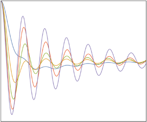
The oscillations are shown in figure 2, where time is normalized by the buoyancy period $T = 2{\rm \pi} /N$, evaluating (2.14) numerically with Mathematica's NIntegrate. Horizontally flat bodies, with $\epsilon < 1$, take several periods to reach their neutral level, while vertically elongated bodies, $\epsilon > 1$, experience symmetrical oscillations almost from the start.

Figure 2.

Exact (solid lines) and asymptotic (dashed lines) free oscillations of (a,c,e,g,i) elliptic cylinders and (b,d,f,h,j) spheroids of aspect ratios (a,b) $\epsilon = 0.2$, (c,d) $\epsilon = 0.5$, (e,f) $\epsilon = 1$, (g,h) $\epsilon = 2$ and (i,j) $\epsilon = 5$, in an inviscid fluid.

In order to model these behaviours analytically, we proceed as in Part 1 for the memory integral and derive the asymptotic expansion of the oscillations for large time $Nt \gg 1$. The analysis is presented in Appendix B. As a rule, here and later in §§ 3 and 4, the expansion combines two terms. One, $\zeta _2$, is present for all parameter values. It is made up of algebraically decaying oscillations at the buoyancy frequency, and – except for the pathological case of the resonance in § 4.1 – dominates ultimately for very large $Nt$. Depending on the case, it may need to be taken into account from the start, or after only a few periods. The other term, $\zeta _1$, is present only in some parameter range. Except for the resonance in § 4.1, it is significant for moderately large $Nt$ and vanishes afterwards.

We have here

(2.18)\begin{equation} \frac{\zeta_1(t)}{\zeta_0} \sim H(1-\epsilon) \exp(-\omega_{s}t),\end{equation}

where $\omega _{s} = N\varOmega _{s}$, and

(2.19)\begin{equation} \varOmega_{s} = \frac{\epsilon}{(1-\epsilon^2)^{1/2}},\end{equation}

which is observed only for $\epsilon < 1$ and gives a gradual exponential return to the neutral level. Also,

(2.20)\begin{equation} \frac{\zeta_2(t)}{\zeta_0} \sim \epsilon \left(\frac{2}{\rm \pi}\right)^{1/2} \frac{\cos(Nt-{\rm \pi}/4)}{(Nt)^{1/2}},\end{equation}

which is observed for all $\epsilon$ and exhibits a decay of the oscillations as $t^{-1/2}$. The superposition of $\zeta _1$ and $\zeta _2$ is shown as a dashed line in figure 2. It provides a satisfactory description of the motion for almost any $t/T$ at $\epsilon < 1$, but requires larger values of $t/T$ as $\epsilon$ increases above $1$. At $\epsilon = 5$, for example, the expansion is valid only for $t/T > 15$, say (outside the displayed range).

2.3. Spheroid

Switching to a spheroid of vertical $z$-axis, with semi-axes $a$ and $b$ along the horizontal and the vertical, respectively, and the same definition $\epsilon = b/a$ of the aspect ratio, the physical behaviour remains the same, but the mathematical analysis is more involved. The added mass coefficient is

(2.21)\begin{equation} C_z(\omega) = \left(1-\frac{N^2}{\omega^2}\right) \frac{D(\varUpsilon)}{1-D(\varUpsilon)},\end{equation}

where the auxiliary variable $\varUpsilon$ is defined as

(2.22)\begin{equation} \varUpsilon = \epsilon \left(1-\frac{N^2}{\omega^2}\right)^{1/2},\end{equation}

and the auxiliary function $D(\varUpsilon )$ as

(2.23)\begin{equation} D(\varUpsilon) = \frac{1}{1-\varUpsilon^2} \left[ 1-\varUpsilon\,\frac{\arccos\varUpsilon}{(1-\varUpsilon^2)^{1/2}} \right]. \end{equation}

The variations of $D(\varUpsilon )$ and $C_z(\omega )$ in the planes of the complex variables $\varUpsilon$ and $\varOmega = \omega /N$ were discussed in Part 1. The transform (2.11) becomes

(2.24)\begin{equation} \frac{\zeta_+(\omega)}{\zeta_0} = \frac{\mathrm{i}}{\omega}\, \frac{\omega^2-N^2\,D(\varUpsilon)}{\omega^2-N^2},\end{equation}

and inverts to

(2.25)\begin{equation} \frac{\zeta_+(t)}{\zeta_0} = \epsilon \int_0^{{\rm \pi}/2} \frac{\cos(Nt\cos\theta)\cos\theta} {(\cos^2\theta+\epsilon^2\sin^2\theta)^{3/2}} \,\mathrm{d}\theta. \end{equation}

For $\epsilon = 1$, namely the sphere, a Weber or Struve function is obtained,

(2.26)\begin{equation} \frac{\zeta_+(t)}{\zeta_0} = \frac{\rm \pi}{2}\,\operatorname{{\boldsymbol{E}}}_1(Nt) = 1-\frac{\rm \pi}{2}\,\operatorname{{\boldsymbol{H}}}_1(Nt),\end{equation}

consistent with Larsen (Reference Larsen1969). For arbitrary $\epsilon$, the use of Jacobi's expansion yields

(2.27)\begin{equation} \frac{\zeta_+(t)}{\zeta_0} = \epsilon \sum_{n=0}^\infty ({-}1)^n\epsilon_n\,{\rm J}_{2n}(Nt) \int_0^{{\rm \pi}/2} \frac{\cos(2n\theta)\cos\theta} {(\cos^2\theta+\epsilon^2\sin^2\theta)^{3/2}} \,\mathrm{d}\theta,\end{equation}

where each integral may be evaluated by a change of variable but does not exhibit a general form for arbitrary $n$ leading to an equivalent of (2.17).

The oscillations in figure 2 exhibit behaviour similar to that of the cylinder, except for a slight overshoot of the neutral level for $\epsilon < 1$. This overshoot is linked to the presence of Dawson's integral $F(t) = \exp (-t^2)\int _0^t\exp (\tau ^2)\,\mathrm {d}\tau$ in the intermediate contribution

(2.28)\begin{equation} \frac{\zeta_1(t)}{\zeta_0} \sim H(1-\epsilon)\, \frac{1-2(\omega_{s}t)^{1/2}\,F[(\omega_{s}t)^{1/2}]} {2^{1/2}(1-\epsilon^2)^{1/2}},\end{equation}

while the ultimate contribution

(2.29)\begin{equation} \frac{\zeta_2(t)}{\zeta_0} \sim \epsilon \left(\frac{\rm \pi}{2}\right)^{1/2} \frac{\cos(Nt-{\rm \pi}/4)}{(Nt)^{1/2}},\end{equation}

is identical up to a factor ${\rm \pi} /2$ to that for the cylinder.

2.4. Comparison with experiment

Several data sets are available in the literature, to which these predictions can be compared. Their characteristics are listed in table 1. The only similarity parameter at this stage is the Keulegan–Carpenter number ${Ke} = \zeta _0/a$, representing the ratio of the oscillation amplitude to the size of the body. As already mentioned, the analysis assumes small oscillation velocity. With $Na$ the only velocity scale, and $N\zeta _0$ the typical oscillation velocity, this condition becomes ${Ke} \ll 1$, namely small displacement of the body compared with its size.

Table 1.

Parameters in figures 3–6 and 8.

Most measurements are for the sphere. Larsen (Reference Larsen1969) and Hurlen (Reference Hurlen2006) used big spheres with relatively small ${Ke}$ from $0.5$ to $2$, while Levitskii & Chashechkin (Reference Levitskii and Chashechkin1999), Chashechkin & Levitskii (Reference Chashechkin and Levitskii2003) and Prikhod'ko & Chashechkin (Reference Prikhod'ko and Chashechkin2006) used smaller spheres with larger ${Ke}$ from $2$ to $5$, say. The comparison with theory, shown in figures 3 and 4, does not exhibit any systematic effect of ${Ke}$. Indeed, Vasil'ev & Chashechkin (Reference Vasil'ev and Chashechkin2009) presented statistical averages over experiments for different values of ${Ke}$, keeping all other parameters constant; the averages were spline-interpolated then resampled. Some experiments belonged to the earlier series by Levitskii, Prikhod'ko and Chashechkin, while others were performed specially by Y. Prikhod'ko for the purpose of the study (A. Vasil'ev, personal communication). The outcome, shown in figure 5, does not differ significantly from the direct measurements in figures 3 and 4, confirming minimal effect of ${Ke}$ if any.

Figure 3.

Comparison of inviscid (blue lines) and viscous (brown lines) theories with the data (circles) in figure 2 of Larsen (Reference Larsen1969) and figure 4.3 of Hurlen (Reference Hurlen2006). Parameters values are given in table 1.

Figure 4.

Same as figure 3 for the data in figures 2 and 7 of Levitskii & Chashechkin (Reference Levitskii and Chashechkin1999), figure 5 of Chashechkin & Levitskii (Reference Chashechkin and Levitskii2003) and figure 2 of Prikhod'ko & Chashechkin (Reference Prikhod'ko and Chashechkin2006).

Figure 5.

Same as figure 3 for the data in figures 1 and 2 of Vasil'ev & Chashechkin (Reference Vasil'ev and Chashechkin2009).

What appears, however, is an increasing discrepancy between theory and experiment as the size of the sphere decreases, independent of ${Ke}$. Viscous damping is the most likely explanation, for which the appropriate similarity parameter is the Stokes number ${St} = Na^2/\nu$ representing the ratio of the viscous time scale $a^2/\nu$ to the buoyancy time scale $1/N$, with $\nu$ the kinematic viscosity. The agreement between theory and experiment is good for ${St} > 1000$, say. As ${St}$ decreases below this value, the oscillations are damped faster than predicted by inviscid theory.

Measurements were done by Hurlen (Reference Hurlen2006) for elliptic cylinders of varying aspect ratio $\epsilon$. In most cases, emphasis was on the rotational motion of the cylinder, whose elliptic cross-section was inclined. The three cases involving the translation of a straight ellipse are shown in figure 6, providing too limited a sample to draw conclusions on the role of $\epsilon$.

Figure 6.

Same as figure 3 for the data in figures 4.5 and 4.6 of Hurlen (Reference Hurlen2006).

2.5. Viscous analysis

The viscous damping of the oscillations of the sphere was considered by Vasil'ev, Kistovich & Chashechkin (Reference Vasil'ev, Kistovich and Chashechkin2007) and Vasil'ev & Chashechkin (Reference Vasil'ev and Chashechkin2009). Using a no-slip boundary condition, the oscillations were obtained as a series

(2.30)\begin{equation} \frac{\zeta_+(t)}{\zeta_0} = \sum_{n=0}^\infty h_n\left(\frac{Nt}{St}\right) {\rm J}_{2n}(Nt), \end{equation}

of the same general form as the inviscid result (2.27), with the functions $h_n$ satisfying an integro-differential system to be solved by the method of multiple scales. Inspection of this system led to the variational representation

(2.31)\begin{equation} \frac{\zeta_+(t)}{\zeta_0} = \operatorname{erf}\left[\alpha\left(\frac{St}{Nt}\right)^{1/2}\right] \sum_{n=0}^\infty\beta_n\,{\rm J}_{2n}(Nt), \end{equation}

with $\operatorname {erf} t$ the error function. The coefficients $\alpha$ and $\beta _n$ had to be set by fit to the measurements. Eventually, only the first term of the series was retained,

(2.32)\begin{equation} \frac{\zeta_+(t)}{\zeta_0} = \operatorname{erf}\left[\alpha\left(\frac{St}{Nt}\right)^{1/2}\right] {\rm J}_0(Nt), \end{equation}

leaving a single coefficient $\alpha$ to set.

We proceed differently, based on the observation by Ermanyuk (Reference Ermanyuk2000, Reference Ermanyuk2002), Ermanyuk & Gavrilov (Reference Ermanyuk and Gavrilov2002a,Reference Ermanyuk and Gavrilovb, Reference Ermanyuk and Gavrilov2003) and Brouzet et al. (Reference Brouzet, Ermanyuk, Moulin, Pillet and Dauxois2017) for the problem considered in § 4, that at sufficiently large ${St}$, say ${St} > 100$, viscous damping is unaffected by the stratification. It is thus the same boundary-layer dissipation that gives the Basset–Boussinesq memory force in a homogeneous fluid. The modelling of this force is recalled in Appendix C, yielding the Fourier transform

(2.33)\begin{equation} F_{v}(\omega) = mN^{1/2}\omega^{3/2} \,\mathrm{e}^{{\rm i}{\rm \pi}/4}\, \frac{B_z}{{St}^{1/2}}\,\zeta(\omega),\end{equation}

where the coefficient $B_z$, equal to $9/2$ for the sphere and $4$ for the circular cylinder, varies with the aspect ration $\epsilon$. The expression of $B_z(\epsilon )$ is given in table 4, and its variations are represented in figure 21. The Fourier transform (2.11) becomes

(2.34)\begin{equation} \frac{\zeta_+(\omega)}{\zeta_0} = \mathrm{i}\, \frac{\omega[1+C_z(\omega)] +\mathrm{e}^{{\rm i}{\rm \pi}/4} (B_z/{St}^{1/2})N^{1/2}\omega^{1/2}} {\omega^2[1+C_z(\omega)]-N^2 +\mathrm{e}^{{\rm i}{\rm \pi}/4} (B_z/{St}^{1/2})N^{1/2}\omega^{3/2}},\end{equation}

where the assumption ${St} \gg 1$ is implicit, and the branch cut away from the singularity $\omega = 0$ is taken vertically downwards.

This gives for the elliptic cylinder

(2.35)\begin{equation} \frac{\zeta_+(\omega)}{\zeta_0} = \mathrm{i}\, \frac{\epsilon\omega+(\omega^2-N^2)^{1/2} +\mathrm{e}^{{\rm i}{\rm \pi}/4} (\epsilon B_z/{St}^{1/2})N^{1/2}\omega^{1/2}} {\omega(\omega^2-N^2)^{1/2}+\epsilon(\omega^2-N^2) +\mathrm{e}^{{\rm i}{\rm \pi}/4} (\epsilon B_z/{St}^{1/2})N^{1/2}\omega^{3/2}},\end{equation}

with inverse transform, obtained by the method of Appendix A,

(2.36)\begin{align} \frac{\zeta_+(t)}{\zeta_0} & = \frac{2}{\rm \pi}\,\epsilon \operatorname{Re} \left\{ \int_0^{{\rm \pi}/2} \frac{\exp(-\mathrm{i}Nt\cos\theta)\sin^2\theta} {\sin^2\theta\cos^2\theta+\epsilon^2 [ \sin^2\theta- \mathrm{e}^{{\rm i}{\rm \pi}/4} (B_z/{St}^{1/2}) \cos^{3/2}\theta ]^2} \,\mathrm{d}\theta \right\} \nonumber\\ & \quad- \frac{\epsilon^2}{\rm \pi}\, \frac{B_z}{{St}^{1/2}} \int_0^\infty \frac{\exp({-}Nt\sinh\alpha)\sinh^{1/2}\alpha\cosh\alpha} {\cosh^2\alpha\,(\sinh\alpha+\epsilon\cosh\alpha)^2+ \epsilon^2(B_z^2/{St}) \sinh^3\alpha} \,\mathrm{d}\alpha. \end{align}

Similarly, for the spheroid we have

(2.37)\begin{equation} \frac{\zeta_+(\omega)}{\zeta_0} = \frac{\mathrm{i}}{\omega}\, \frac{\omega^2-N^2\,D(\varUpsilon)+ \mathrm{e}^{{\rm i}{\rm \pi}/4} (B_z/{St}^{1/2})N^{1/2}\omega^{3/2} [1-D(\varUpsilon)]} {\omega^2-N^2+ \mathrm{e}^{{\rm i}{\rm \pi}/4} (B_z/{St}^{1/2})N^{1/2}\omega^{3/2} [1-D(\varUpsilon)]}, \end{equation}

with inverse transform

(2.38) \begin{align} \frac{\zeta_+(t)}{\zeta_0} & = \epsilon \operatorname{Re} \left\{ \vphantom{\left\{\left[\frac{\epsilon B_z}{{St}^{1/2}}\right]^2\right\}^{{-}1}} \int_0^{{\rm \pi}/2} \frac{\exp(-\mathrm{i}Nt\cos\theta)} {(1+\epsilon^2\tan^2\theta)^{3/2}} \tan^2\theta \left\{ \vphantom{\left[\frac{\epsilon B_z}{{St}^{1/2}}\right]^2} \mathrm{i}\,\frac{{\rm \pi}^2}{4}\, \frac{\epsilon^2B_z^2}{St}\, \frac{\cos\theta}{(1+\epsilon^2\tan^2\theta)^3} + \left[ \vphantom{\frac{\epsilon B_z}{{St}^{1/2}}} \sin\theta \right. \right. \right. \nonumber\\ & \quad -\! \left.\left.\left.\mathrm{e}^{{\rm i}{\rm \pi}/4}\,\frac{\epsilon B_z}{{St}^{1/2}} \cos^{1/2}\theta\, \frac{\operatorname{arcsinh}(\epsilon\tan\theta)+ \epsilon\tan\theta (1+\epsilon^2\tan^2\theta)^{1/2}} {(1+\epsilon^2\tan^2\theta)^{3/2}} \right]^2 \right\}^{{-}1} \mathrm{d}\theta \right\} \nonumber\\ &\quad -\frac{\epsilon^2}{\rm \pi}\, \frac{B_z}{{St}^{1/2}} \int_0^{\operatorname{arctanh}\epsilon} \frac{\exp({-}Nt\sinh\alpha)}{\sinh^{3/2}\alpha} \cosh\alpha \left\{\frac{\epsilon^2B_z^2}{St} \sinh\alpha\right. \nonumber\\ & \quad + \left. \frac{\cosh^2\alpha\,(\epsilon^2\coth^2\alpha-1)^3} {[\epsilon\coth\alpha\,(\epsilon^2\coth^2\alpha-1)^{1/2}- \operatorname{arccosh}(\epsilon\coth\alpha)]^2} \vphantom{\frac{\epsilon^2B_z^2}{St}}\right\}^{{-}1} \mathrm{d}\alpha \nonumber\\ & \quad- \frac{\epsilon^2}{\rm \pi}\, \frac{B_z}{{St}^{1/2}} \int_{\operatorname{arctanh}\epsilon}^\infty \frac{\exp({-}Nt\sinh\alpha)}{\sinh^{3/2}\alpha} \cosh\alpha\left\{ \frac{\epsilon^2B_z^2}{St} \sinh\alpha\right. \nonumber\\ & \quad +\left. \frac{\cosh^2\alpha\,(1-\epsilon^2\coth^2\alpha)^3} {[\arccos(\epsilon\coth\alpha)-\epsilon\coth\alpha\, (1-\epsilon^2\coth^2\alpha)^{1/2}]^2} \vphantom{\frac{\epsilon^2B_z^2}{St}}\right\}^{{-}1} \mathrm{d}\alpha, \end{align}

where for $\epsilon > 1$, the third integral is absent and the second goes from $0$ to $\infty$.

These expressions of the inverse transforms are somewhat tedious compared with their inviscid counterparts, and they do not provide any insight into the physics of the oscillations. They are, however, computationally efficient, since the Fourier integral over the semi-infinite range $|\omega | > N$, brought in by viscosity, is turned into an integral with an exponentially decaying integrand. Each plot is then obtained within seconds. Unfortunately, the associated deformation of contour is not always possible, as discussed in Appendix A. The affected cases reveal themselves immediately, as the application of (2.36) or (2.38) to them gives an oscillation that does not start from $1$ at $t = 0$.

To deal with these cases, we take advantage of the causal nature of $\zeta _+(t)$ and rewrite it as an inverse Laplace transform

(2.39)\begin{equation} \zeta_+(t) = \frac{1}{2\mathrm{i}{\rm \pi}} \int_{c-\mathrm{i}\infty}^{c+\mathrm{i}\infty} \zeta_+(\omega = \mathrm{i}p) \exp(pt)\,\mathrm{d}p,\end{equation}

where the real number $c$ is on the right of all singularities of $\zeta _+(\omega = \mathrm {i}p)$. This transform is evaluated numerically using Mathematica's InverseLaplaceTransform, which implements a variety of standard methods (Davies & Martin Reference Davies and Martin1979; Abate, Choudhury & Whitt Reference Abate, Choudhury and Whitt2000; Cohen Reference Cohen2007). In so doing, the calculation time is multiplied by a factor $50$ to $200$, yielding $10$ to $30$ minutes, say, sometimes even more, for a single plot. For the limited number of affected cases this was deemed acceptable, but it was pointed out and demonstrated by S. Llewellyn Smith (personal communication) that implementing den Iseger's (Reference den Iseger2006) algorithm in MATLAB brings the calculation time down to a few seconds.

The oscillations are shown in figure 7 for Stokes number ${St} = 500$. Compared with figure 2, viscosity is seen to damp the oscillations rapidly and increase their period slightly. To model this evolution, we resort again to asymptotics. For the cylinder, (2.18) and (2.20) become

(2.40)\begin{equation} \frac{\zeta_1(t)}{\zeta_0} \sim H(1-\epsilon) \exp (-\omega_{s}t) \cos \left[ Nt\, \frac{B_z}{{St}^{1/2}}\, \frac{\epsilon^{5/2}}{(1-\epsilon^2)^{5/4}} \right] \end{equation}

and

(2.41)\begin{equation} \frac{\zeta_2(t)}{\zeta_0} \sim \epsilon \cos\left(Nt-\frac{\rm \pi}{4}\right) \left\{ \left(\frac{2}{{\rm \pi} Nt}\right)^{1/2}- \frac{\epsilon B_z}{{St}^{1/2}} \exp\left(\epsilon^2B_z^2\,\frac{Nt}{2{St}}\right) \operatorname{erfc}\left[\epsilon B_z\left(\frac{Nt}{2{St}}\right)^{1/2}\right] \right\}, \end{equation}

respectively. Similarly, for the spheroid, (2.28) and (2.29) become

(2.42)\begin{align} \frac{\zeta_1(t)}{\zeta_0} & \sim \frac{{\rm \pi}^{2/3}}{3}\,\frac{{St}^{1/6}}{B_z^{1/3}}\, \frac{H(1-\epsilon)}{\epsilon^{1/2}(1-\epsilon^2)^{1/12}} \exp \left[ -\omega_{s}t -\frac{{\rm \pi}^{2/3}}{4}\, Nt\,\frac{B_z^{2/3}}{{St}^{1/3}}\, \frac{\epsilon^2}{(1-\epsilon^2)^{4/3}} \right] \nonumber\\ & \quad\times \cos \left[ \frac{3^{1/2}{\rm \pi}^{2/3}}{4}\,Nt\, \frac{B_z^{2/3}}{{St}^{1/3}}\, \frac{\epsilon^2}{(1-\epsilon^2)^{4/3}} +\frac{\rm \pi}{6} \right] \end{align}

and

(2.43) \begin{align} \frac{\zeta_2(t)}{\zeta_0} &\sim \epsilon \cos\left(Nt-\frac{\rm \pi}{4}\right) \left\{\vphantom{\left.\quad -\, \frac{{\rm \pi}^2}{4}\,\frac{\epsilon B_z}{{St}^{1/2}} \exp\left(\frac{{\rm \pi}^2}{4}\,\epsilon^2B_z^2\,\frac{Nt}{2{St}}\right) \operatorname{erfc}\left[\frac{\rm \pi}{2}\,\epsilon B_z\left(\frac{Nt}{2{St}}\right)^{1/2}\right] \right\}} \left(\frac{\rm \pi}{2Nt}\right)^{1/2}\right.\nonumber\\ &\left.\quad -\, \frac{{\rm \pi}^2}{4}\,\frac{\epsilon B_z}{{St}^{1/2}} \exp\left(\frac{{\rm \pi}^2}{4}\,\epsilon^2B_z^2\,\frac{Nt}{2{St}}\right) \operatorname{erfc}\left[\frac{\rm \pi}{2}\,\epsilon B_z\left(\frac{Nt}{2{St}}\right)^{1/2}\right] \right\}, \end{align}

respectively.

Figure 7.

Same as figure 2 in a viscous fluid at Stokes number ${St} = 500$.

The general trend (2.40) for the cylinder includes a low-frequency modulation added by viscosity, while (2.42) for the spheroid points out a singularity of the inviscid limit ${St} \to \infty$. A more physical result is the transition, described by (2.41) and (2.43), between two ultimate regimes: one inviscid, for ${St} \gg Nt \gg 1$, given by (2.20) and (2.29), made of buoyancy oscillations decaying as $t^{-1/2}$; and another viscous, for $Nt \gg {St} \gg 1$, given by

(2.44)\begin{equation} \frac{\zeta_2(t)}{\zeta_0} \sim \left(\frac{2}{\rm \pi}\right)^{1/2}\, \frac{St}{\epsilon B_z^2} \frac{\cos(Nt-{\rm \pi}/4)}{(Nt)^{3/2}} \end{equation}

for the cylinder, and

(2.45)\begin{equation} \frac{\zeta_2(t)}{\zeta_0} \sim \left(\frac{2}{\rm \pi}\right)^{3/2} \frac{St}{\epsilon B_z^2}\, \frac{\cos(Nt-{\rm \pi}/4)}{(Nt)^{3/2}}\end{equation}

for the spheroid, made up of oscillations decaying faster as $t^{-3/2}$.

The comparison of these asymptotics with the exact solution in figure 7 is less successful than in the inviscid case. It becomes even inconclusive for $\epsilon = 5$: the asymptotics start by underestimating the amplitude, get it right after about ten periods, then overestimate it; all along, they underestimate the period slightly so that after ten periods there is a one-period shift with the actual oscillations. The mathematical explanation of this failure is discussed in Appendix B. The asymptotics must thus be viewed only as a qualitative tool, to point out the effects of viscosity.

The comparison with experiment in figures 3–6 shows that viscous effects are significant for ${St} < 1000$ and are described satisfactorily by the present model in most cases. In figures 4(a,b,e) and 5(a,b,e,g), in particular, the model appears in full quantitative agreement with the measurements after one or two periods. The prediction of an ultimate decay as $t^{-3/2}$ is reminiscent of the observation by Biró et al. (Reference Biró, Szabó, Gyüre, Jánosi and Tél2008), in experiments carried over $400$ buoyancy periods, of a power decay as $t^{-3/2}$ during the first $200$ periods. This is confirmed by the comparison with their data in figure 8. These experiments, involving small spheres dropped at the surface of a $50\ \mathrm {cm}$ high tank, were originally thought irrelevant for the present study owing to their large initial displacement (${St} = 66$ and ${Ke} = 33$ in figure 8), and suited instead for a description by the approach of Winant (Reference Winant1974), as discussed in § 1. The good agreement with small-amplitude theory may thus be entirely coincidental.

Figure 8.

(a) Global and (b) local comparisons of inviscid (blue line) and viscous (brown lines) theories with the data (circles) for run 3 in figure 2 of Biró et al. (Reference Biró, Szabó, Gyüre, Jánosi and Tél2008). The other runs (1, 2 and 4) give similar results. In (b), only the viscous theory is shown, with the solid line representing the exact result (2.37) and (2.39), the dashed line the uniform expansion (2.43), and the dotted line the non-uniform expansion (2.45). The original data were shifted between runs to achieve the best fit in the period $2 < t/T < 3$, making the slight time shift between the data and the theory insignificant.

Winant (Reference Winant1974) dropped ping-pong balls of radius $a = 1.875\ \mathrm {cm}$ at the surface of a $1\ \mathrm {m}$ high tank stratified with buoyancy frequency approximately $N = 1\ \mathrm {s}^{-1}$. The balls were partially filled with salt water to be neutrally buoyant at the mid-height of the tank, so that for drop height $\zeta _0 = 50\ \mathrm {cm}$, the Stokes number was ${St} = 350$ and the Keulegan–Carpenter number was ${Ke} = 30$. The observed first overshoot was significantly smaller than that, about half the drop height, predicted by the present theory. Unfortunately the rescalings in figure 7 of Winant (Reference Winant1974), and the absence of any indication on the time taken by the ball to reach its neutral level, prohibit the same comparison as for Biró et al. (Reference Biró, Szabó, Gyüre, Jánosi and Tél2008). Cairns et al. (Reference Cairns, Munk and Winant1979) dropped a neutrally buoyant capsule of radius $a = 41.5\ \mathrm {cm}$ into Lake Tahoe, where it sank to an equilibrium depth of about $\zeta _0 = 240\ \mathrm {m}$, at which the buoyancy frequency was $N = 2\times 10^{-4}\ \mathrm {s}^{-1}$, so that ${St} = 30$ and ${Ke} = 600$, and observed a first overshoot of approximately one capsule diameter.

3.1. Inviscid analysis

The modelling of this set-up follows the same lines as in § 2. The diver combines a fixed volume $\mathcal {V}_{g}$ of glass with density $\rho _{g}$, and a varying volume $\mathcal {V}_{a}$ of air with negligible density. Its mass $m = \rho _{g}\mathcal {V}_{g}$ is thus constant, while the mass of the displaced fluid $m_{f} = \rho _0(\mathcal {V}_{g}+\mathcal {V}_{a})$ varies. The vertical origin $z = 0$ is taken at the neutral level where the weight of the diver is exactly opposed by Archimedes’ force, so that

(3.1)\begin{equation} m_{f}(0) = \rho_0(0)\,[\mathcal{V}_{g}+\mathcal{V}_{a}(0)] = m = \rho_{g}\mathcal{V}_{g}, \end{equation}

while the piston is at rest at the vertical position $h = 0$ (with a different vertical origin). The piston then moves to a new position $h$, causing the diver to reach the position $\zeta$. Both displacements are assumed small. The ambient pressure changes hydrostatically to $p_0(\zeta ) = p_0(0)+\rho _0(0)\,g(h-\zeta )$, and the entrapped air volume changes adiabatically to

(3.2)\begin{equation} \mathcal{V}_{a}(\zeta) = \mathcal{V}_{a}(0) \left[ 1-\frac{g}{\gamma}\, \frac{\rho_0(0)}{p_0(0)}\,(h-\zeta) \right], \end{equation}

with $\gamma$ the ratio of specific heats of air. Meanwhile, the ambient density has changed to $\rho _0(\zeta )$ given in (2.2). The new displaced fluid mass is

(3.3)\begin{equation} m_{f}(\zeta) = \rho_0(\zeta)\,[\mathcal{V}_{g}+\mathcal{V}_{a}(\zeta)] = m \left( 1-\frac{N^2-\omega_0^2}{g}\,\zeta-\frac{\omega_0^2}{g}\,h \right), \end{equation}

where

(3.4a,b)\begin{equation} \delta = 1-\frac{\rho_0(0)}{\rho_{g}}, \quad \omega_0 = g\left[\frac{\delta}{\gamma}\,\frac{\rho_0(0)}{p_0(0)}\right]^{1/2}. \end{equation}

The diver is acted upon by the hydrostatic force

(3.5)\begin{equation} F_{s}(t) ={-}m(N^2-\omega_0^2)\,\zeta(t)-m\omega_0^2\,h(t), \end{equation}

together with the hydrodynamic force (2.6), yielding the equation of motion

(3.6)\begin{equation} [m+m_z(t)\ast]\,\frac{\mathrm{d}^2\zeta}{\mathrm{d}t^2} +m(N^2-\omega_0^2)\,\zeta(t) ={-}m\omega_0^2\,h(t),\end{equation}

first derived by Le Gal et al. (Reference Le Gal, Castillo Morales, Hernandez-Zapata and Ruiz Chavarria2022). As remarked by them, the diver is a stable oscillator provided that $\omega _0 < N$, which is the case considered here. Taking Fourier transforms in time, we introduce the added mass coefficient $C_z(\omega )$, and write $m_z(\omega ) = m_{f}\,C_z(\omega ) \approx m\,C_z(\omega )$, consistent with the Boussinesq approximation.

In the experiments of Le Gal et al. (Reference Le Gal, Castillo Morales, Hernandez-Zapata and Ruiz Chavarria2022), the piston started by performing sinusoidal oscillations $h(t) = h_0\exp (-\mathrm {i}\omega _{f}t)$ of frequency $\omega _{f}$, causing the diver to oscillate with it as $\zeta (t) = \zeta _0\exp (-\mathrm {i}\omega _{f}t)$, where

(3.7)\begin{equation} \frac{\zeta_0}{h_0} = \frac{\omega_0^2} {\omega_{f}^2[1+C_z(\omega_{f})]+\omega_0^2-N^2},\end{equation}

in phase with the piston in the supercritical case $\omega _{f} > N$, and out of phase in the subcritical case $\omega _{f} < N$.

The piston was then stopped at a random instant, and the free oscillations of the diver were recorded after it reached its next peak, shown with a red dot in figure 9 (P. Le Gal, personal communication). For lack of a better way to model this process, we assume that the stop took place when the diver was at a peak. We thus set $t = 0$ at the stop, and write $h_0 = A\exp (-\mathrm {i}\phi )$, where the real positive $A$ represents the amplitude of the piston's oscillations, and $\phi$ their initial phase, adjusting $\phi$ to make $\zeta _0$ real positive in (3.7). As in § 2, the motion of the diver is decomposed as

(3.8a,b)\begin{equation} \zeta(t) = \zeta_0\exp(-\mathrm{i}\omega_{f}t)\,H({-}t)+\zeta_+(t), \quad \zeta(\omega) ={-}\frac{\mathrm{i}\zeta_0}{\omega-\omega_{f}-\mathrm{i}0} +\zeta_+(\omega), \end{equation}

with $\zeta _+(t)$ causal and $\zeta _+(\omega )$ analytic in the upper half-plane, and given by

(3.9)\begin{equation} \frac{\zeta_+(\omega)}{h_0} = \frac{\mathrm{i}}{\omega-\omega_{f}} \left\{ \frac{\zeta_0}{h_0} - \frac{\omega_0^2} {\omega^2[1+C_z(\omega)] +\omega_0^2-N^2} \right\}. \end{equation}

To go further, a representation of the diver is required. No analytical result exists for the added mass of a finite-length cylinder. Le Gal et al. (Reference Le Gal, Castillo Morales, Hernandez-Zapata and Ruiz Chavarria2022) used the results of Voisin (Reference Voisin2007) for a sphere, adding adjustable coefficients and power laws to fit the experiments. We investigate whether a more predictive approach is possible, based on an approximate representation of the shape of the diver.

It is common practice in homogeneous fluids to model anisotropic bodies, either big (Korotkin Reference Korotkin2009) or small (Voth & Soldati Reference Voth and Soldati2017), as spheroids. In naval hydrodynamics, for which the bodies are usually elongated and streamlined, the equivalent spheroid has the same axial length and volume as the body (Korotkin Reference Korotkin2009, § 3.5.2). The situation here is different, with the main contribution to added mass coming from the blunt ends of the diver (P. Le Gal, personal communication). For rod-like particles, in the creeping flow regime, different recommendations have been made depending on the motion of the rod: for translation, the equivalent spheroid has the same axial and transverse lengths as the rod (Weinheimer Reference Weinheimer1987); for rotation, the spheroid has an axial to transverse aspect ratio equal to $1.14 \epsilon ^{0.844}$, with $\epsilon$ the aspect ratio of the rod (Harris & Pittman Reference Harris and Pittman1975).

Loewenberg (Reference Loewenberg1993a,Reference Loewenbergb) considered the low- and high-frequency translational oscillations of a finite-length cylinder, looking at Stokes drag, added mass and the Basset–Boussinesq force, then studied the flow in greater detail (Loewenberg Reference Loewenberg1994a,Reference Loewenbergb). The way in which these three components of fluid resistance combine their effects, and the way in which they vary with the frequency, were seen to be the same for the cylinder and for a spheroid of the same aspect ratio $\epsilon$, provided that $0.1 < \epsilon < 10$. However, the actual value of added mass and its variations with $\epsilon$ were predicted with only mild accuracy for transverse oscillations, and with poor accuracy for axial oscillations. This is in agreement with the above observation by P. Le Gal.

In the following, for lack of a better analytical model, we consider a spheroid with the same axial length $2b$ as the diver and a volume-preserving transverse radius $a$ equal to $(3/2)^{1/2} \approx 1.22$ times the radius of the diver. With $C_z(\omega )$ given in (2.21), the amplitude of the oscillations in the forced regime becomes

(3.10)\begin{equation} \frac{\zeta_0}{h_0} = \frac{\omega_0^2[1-D(\varUpsilon_{f})]} {\omega_{f}^2-N^2 +\omega_0^2[1-D(\varUpsilon_{f})]},\end{equation}

where $\varUpsilon _{f}$ denotes the value of the variable (2.22) at $\omega = \omega _{f}$, and the Fourier transform of the free oscillations afterwards becomes

(3.11)\begin{equation} \frac{\zeta_+(\omega)}{h_0} = \frac{\mathrm{i}}{\omega-\omega_{f}} \left\{ \frac{\zeta_0}{h_0} - \frac{\omega_0^2[1-D(\varUpsilon)]} {\omega^2-N^2 +\omega_0^2[1-D(\varUpsilon)]} \right\}.\end{equation}

Inverting this transform as before, we obtain

(3.12) \begin{align} \frac{\zeta_+(t)}{h_0} & = \mathrm{i}\operatorname{Im} \left[ \frac{\zeta_0}{h_0} \right] \exp(-\mathrm{i}\omega_{f}t) + \frac{1}{\epsilon\varOmega_0^2} {\unicode{x2A0D}}_0^{\pi/2} \frac{\cos\theta\cos(Nt\cos\theta) -\mathrm{i}\varOmega_{f}\sin(Nt\cos\theta)} {\varOmega_{f}^2-\cos^2\theta} \nonumber\\ & \quad \times \left\{ \vphantom{\left. \left.\vphantom{\frac{\sin\theta\cos\theta}{\epsilon\varOmega_0^2}} \times(1+\epsilon^2\tan^2\theta)^{3/2} \right]^2\right\}^{{-}1}} \frac{\pi^2}{4}+ \left[ \operatorname{arcsinh}(\epsilon\tan\theta)+ \epsilon\tan\theta\,(1+\epsilon^2\tan^2\theta)^{1/2}- \frac{\sin\theta\cos\theta}{\epsilon\varOmega_0^2} \right. \right. \nonumber\\ & \quad \times\! \left. \left. (1+\epsilon^2\tan^2\theta)^{3/2} \vphantom{\frac{\sin\theta\cos\theta}{\epsilon\varOmega_0^2}}\right]^2\right\}^{{-}1} \sin^2\theta\cos\theta (1+\epsilon^2\tan^2\theta)^{3/2}\,\mathrm{d}\theta, \end{align}

where $\varOmega _0 = \omega _0/N$ and $\varOmega _{f} = \omega _{f}/N$. For subcritical forcing, $\varOmega _{f} < 1$, the first term on the right-hand side is non-zero, and the integral in the second term must be interpreted as a principal value, denoted by a stroke. For supercritical forcing, $\varOmega _{f} > 1$, the first term vanishes and the integral becomes regular.

To exhibit the physical content of this expression, we turn again to its expansion for large time, $Nt \gg 1$. The intermediate contribution for moderately large $Nt$ is an exponentially damped oscillation

(3.13)\begin{align} \frac{\zeta_1(t)}{h_0} & \sim 2\epsilon\, \frac{\exp(-\omega_{i}t)} {\varOmega_{r}^2+(\varOmega_{i}-\mathrm{i}\varOmega_{f})^2}\, [\varOmega_{r}\operatorname{Re}-(\varOmega_{i}-\mathrm{i}\varOmega_{f})\operatorname{Im}] \nonumber\\ & \quad \times \left\{ \frac{\varUpsilon_{c}^2-1} {2(\varOmega_0^2-1)(\epsilon^2-\varUpsilon_{c}^2)^2+ \epsilon^2-\varUpsilon_{c}^2+2\epsilon^2(\epsilon^2-1)}\, \frac{\varUpsilon_{c}^2\exp(-\mathrm{i}\omega_{r}t)} {(\epsilon^2-\varUpsilon_{c}^2)^{1/2}} \right\}, \end{align}

where $\omega _{r} = N\varOmega _{r}$ and $\omega _{i} = N\varOmega _{i}$, and the real and imaginary parts apply to the term in curly braces afterwards. Here, $\varUpsilon _{c}$ and $\overline {\varUpsilon _{c}}$ are the complex conjugate solutions of the equation

(3.14)\begin{equation} \frac{\varUpsilon^2}{\epsilon^2-\varUpsilon^2}+\varOmega_0^2[1-D(\varUpsilon)] = 0, \end{equation}

with $\operatorname {Re}\varUpsilon _{c} < 0$ and $\operatorname {Im}\varUpsilon _{c} > 0$, and $\pm \varOmega _{r}-\mathrm {i}\varOmega _{i}$ are the associated reduced frequencies, with

(3.15)\begin{equation} \varOmega_{r}-\mathrm{i}\varOmega_{i} = \frac{\epsilon}{(\epsilon^2-\varUpsilon_{c}^2)^{1/2}},\end{equation}

and the determination of the square root is chosen such that $0 < \varOmega _{r} < 1$ and $\varOmega _{i} > 0$. The ultimate contribution for very large $Nt$ is the buoyancy oscillation

(3.16)\begin{equation} \frac{\zeta_2(t)}{h_0} \sim \left(\frac{2}{\rm \pi}\right)^{3/2} \frac{1}{\epsilon\varOmega_0^2(\varOmega_{f}^2-1)}\, \frac{\sin(Nt-{\rm \pi}/4) +\mathrm{i}\varOmega_{f}\cos(Nt-{\rm \pi}/4)} {(Nt)^{3/2}},\end{equation}

decaying as $t^{-3/2}$.

Accordingly, once the forcing has stopped, the diver starts by performing oscillations $\zeta _1$ of frequency $\omega _{r}$ and damping rate $\omega _{i}$, before oscillations $\zeta _2$ of frequency $N$ and amplitude decaying as $t^{-3/2}$ manifest themselves, to eventually take over. This evolution is shown in figure 10 for two cases, one subcritical ($\varOmega _{f} = 0.8$) and the other supercritical ($\varOmega _{f} = 1.2$). The contribution $\zeta _1$, with $\varOmega _{r} = 0.847$ and $\varOmega _{i} = 0.088$ for these $\epsilon$ and $\varOmega _0$, is shown alone for $t/T < 4$ in the subcritical case, and $t/T < 2.1$ in the supercritical case; then $\zeta _2$ is added at later times. The transition between a first regime with dominant $\zeta _1$ and a second regime with dominant $\zeta _2$ takes place during the periods $11 < t/T < 12$ in the subcritical case and $6 < t/T < 7$ in the supercritical case.

Figure 10.

Exact (solid lines) and asymptotic (dashed lines) free oscillations of a diver of aspect ratio $\epsilon = 2$ and intrinsic frequency $\varOmega _0 = 1/2$ after forcing at the frequencies (a) $\varOmega _{f} = 0.8$ and (b) $\varOmega _{f} = 1.2$.

These theoretical predictions are now compared with the measurements in figures 3 and 4 of Le Gal et al. (Reference Le Gal, Castillo Morales, Hernandez-Zapata and Ruiz Chavarria2022), for which the fluid was linearly stratified with buoyancy frequency $N = 1.6\ \mathrm {s}^{-1}$. The diver had axial length $2b = 35\ \mathrm {mm}$ and transverse radius $6.25\ \mathrm {mm}$, yielding $a = 7.65\ \mathrm {mm}$ and $\epsilon = 2.3$ for the equivalent spheroid. The effective glass density, taking into account the fluid entrapped under the air pocket and transported with the diver, was $\rho _{g} = 1445\ \mathrm {kg}\ \mathrm {m}^{-3}$. The density of the fluid was $\rho _0(0) = 1030\ \mathrm {kg}\ \mathrm {m}^{-3}$ at the neutral level. The experiments were performed in Mexico City where the atmospheric pressure was $77\ \mathrm {kPa}$, yielding $\omega _0 = 0.5062\ \mathrm {s}^{-1}$ (P. Le Gal, personal communication) and $\varOmega _0 = 0.32$. The piston oscillated with amplitude $A = 28\ \mathrm {mm}$, corrected for surface tension.

Figure 11 compares the forced response (3.10) with its measurement. The position of the peak is predicted reasonably well, at a frequency slightly smaller than the buoyancy frequency, consistent with $\varOmega _{r} = 0.956$ and $\varOmega _{i} = 0.055$ for these $\epsilon$ and $\varOmega _0$, but the value of the peak is overpredicted by a factor of about $3$. The free oscillations (3.12) are compared with their measurements in figure 12, showing that the damping is underpredicted together with the frequency. Again, the necessity arises of taking viscous dissipation into account.

Figure 11.

Experimental data (circles) for the forced oscillations of the diver in figure 3 of Le Gal et al. (Reference Le Gal, Castillo Morales, Hernandez-Zapata and Ruiz Chavarria2022), and comparison with inviscid theory (blue line), viscous theory for Basset–Boussinesq damping (red line), and viscous theory for Stokes damping using the predicted (brown line) and estimated (green line) values of the resistance tensor.

Figure 12.

Experimental data (black lines) in figure 4 of Le Gal et al. (Reference Le Gal, Castillo Morales, Hernandez-Zapata and Ruiz Chavarria2022) for the free oscillations of the diver after (a) subcritical and (b) supercritical forcing, and comparison with inviscid (blue lines) and viscous (brown lines) theories. The data are those appearing after the red dots in figure 9.

3.2. Viscous analysis

With $\nu = 0.01\ \mathrm {cm}^2\ \mathrm {s}^{-1}$, the value of the Stokes number ${St} = 94$ suggests the same dissipative force (2.33), of the Basset–Boussinesq type, as in § 2.5, yielding the forced response

(3.17)\begin{equation} \frac{\zeta_0}{h_0} = \frac{\omega_0^2[1-D(\varUpsilon_{f})]} {\omega_{f}^2-N^2 +[\omega_0^2+\mathrm{e}^{{\rm i}{\rm \pi}/4}\, (B_z/{St}^{1/2})N^{1/2}\omega_{f}^{3/2}] [1-D(\varUpsilon_{f})]}.\end{equation}

The comparison with experiment in figure 11, using the value of $B_z(\epsilon )$ taken from table 4, invalidates this assumption, consistent with the observation by Le Gal et al. (Reference Le Gal, Castillo Morales, Hernandez-Zapata and Ruiz Chavarria2022) that damping is of the Stokes resistance type. The dissipative force becomes

(3.18)\begin{equation} F_{v}(\omega) = \mathrm{i} mN\omega\, \frac{R_z}{St}\,\zeta(\omega),\end{equation}

yielding the response

(3.19)\begin{equation} \frac{\zeta_0}{h_0} = \frac{\omega_0^2[1-D(\varUpsilon_{f})]} {\omega_{f}^2-N^2 +[\omega_0^2+\mathrm{i}(R_z/{St})N\omega_{f}] [1-D(\varUpsilon_{f})]}.\end{equation}

This formula, either taking $R_z(\epsilon )$ from table 4 or using its estimation by Le Gal et al. (Reference Le Gal, Castillo Morales, Hernandez-Zapata and Ruiz Chavarria2022) as $\lambda _z/m = N(R_z/{St}) = 0.16\ \mathrm {s}^{-1}$, improves the comparison significantly, regarding both the position of the peak and its value. Agreement is better using the estimated coefficient, which gives a peak value of about $1.6$ times its measurement, thus showing that, contrary to the Basset–Boussinesq force, Stokes damping is affected significantly by the stratification.

Retaining this model, the Fourier transform (3.11) becomes

(3.20)\begin{equation} \frac{\zeta_+(\omega)}{h_0} = \frac{\mathrm{i}}{\omega-\omega_{f}} \left\{ \frac{\zeta_0}{h_0} - \frac{\omega_0^2[1-D(\varUpsilon)]} {\omega^2-N^2 +[\omega_0^2+\mathrm{i}(R_z/{St})N\omega] [1-D(\varUpsilon)]} \right\}.\end{equation}

Numerical inversion and comparison with experiment in figure 12 show that the addition of Stokes resistance leads to a better prediction of the amplitude of the oscillations, but does not arrange the prediction of their frequency, which remains fully off.

A first explanation is the inadequacy of the model of the diver as a spheroid. This model, however, gives acceptable results for the frequency response. A second explanation is the random time at which the forcing is stopped, which the theory cannot account for.

4.1. Inviscid analysis

The set-up involves a cross-shaped pendulum, with one arm horizontal along the surface of the tank, and the other arm vertical. The body is attached at the lower end of the vertical arm, and a movable counterweight is fitted at its upper end. The length $L$ from the axis of the pendulum to the centroid of the body is large enough for the motion of the body to be considered as a horizontal translation, for which the ratio $M = J/L^2$, with $J$ the moment of inertia of the whole system (pendulum, body and counterweight), acts as a generalized inertia. The immersed part of the pendulum is streamlined, such that its volume is less than $1\,\%$ of the volume of the body, and its added mass may be neglected. The restoring force acting on the pendulum depends on the distance of the counterweight to the axis. It is measured prior to the experiment by in situ static calibration, yielding the restoring coefficient $K$, and from it the eigenfrequency $\omega _0 = (K/M)^{1/2}$.

At the start of the experiment, an impulsive force is applied,

(4.1)\begin{equation} F_{e}(t) = MN\xi_0\,\delta(t), \end{equation}

with $\delta (t)$ the Dirac delta function, setting the pendulum into motion. The pendulum then oscillates under the combined effects of the hydrodynamic force

(4.2)\begin{equation} F_{d}(t) ={-}m_x(t)\ast\frac{\mathrm{d}^2\xi}{\mathrm{d}t^2}, \end{equation}

with $m_x(t)$ the added mass of the body and $\xi$ its horizontal displacement, and the restoring force

(4.3)\begin{equation} F_{r}(t) ={-}K\,\xi(t). \end{equation}

Its motion satisfies the equation

(4.4)\begin{equation} [M+m_x(t)\ast]\,\frac{\mathrm{d}^2\xi}{\mathrm{d}t^2} +K\,\xi(t) = MN\xi_0\,\delta(t).\end{equation}

Taking Fourier transforms in time and introducing the mass $m_{f}$ of the displaced fluid, its ratio $\sigma = m_{f}/M$ to the inertia of the system and the added mass coefficient $C_x(\omega ) = m_x(\omega )/m_{f}$, we obtain

(4.5)\begin{equation} \frac{\xi(\omega)}{\xi_0} = \frac{N}{\omega_0^2-\omega^2[1+\sigma\,C_x(\omega)]},\end{equation}

allowing the deduction of $C_x(\omega )$ from the measurement of $\xi (\omega )$.

The experimental record of the oscillations was given in two cases, a circular cylinder (Ermanyuk Reference Ermanyuk2000) and a diamond-shaped cylinder (Ermanyuk & Gavrilov Reference Ermanyuk and Gavrilov2002b). We consider an elliptic cylinder of aspect ratio $\epsilon$, for which

(4.6)\begin{equation} C_x(\omega) = \epsilon \left(1-\frac{N^2}{\omega^2}\right)^{1/2},\end{equation}

so that

(4.7)\begin{equation} \frac{\xi(\omega)}{\xi_0} = \frac{N} {\omega_0^2-\omega^2-\epsilon\sigma\omega(\omega^2-N^2)^{1/2}}.\end{equation}

A new feature, compared with the free oscillations in § 2.1, is the existence, in the plane of the complex variable $\varOmega = \omega /N$, of poles that are not only imaginary, like $-\mathrm {i}\varOmega _{s}$ previously, but also complex or even real, implying a resonance. These poles are created by the presence of the intrinsic frequency $\varOmega _0 = \omega _0/N$ in the system. To find them, we look for the solutions of the squared equation $(\varOmega _0^2 -\varOmega ^2)^2 = \epsilon ^2\sigma ^2\varOmega ^2(\varOmega ^2-1)$, then check which of these satisfy the original equation $\varOmega _0^2 -\varOmega ^2 = \epsilon \sigma \varOmega (\varOmega ^2-1)^{1/2}$. For complex solutions, this means satisfying the conditions $|\operatorname {Re}\varOmega | < 1$ and $\operatorname {Im}\varOmega < 0$, which ensures that the solutions belong to the proper Riemann sheet.

The poles are linked to the sign of

(4.8)\begin{equation} \varDelta = 4\varOmega_0^2(\varOmega_0^2-1)+\epsilon^2\sigma^2 = (2\varOmega_0^2-1)^2+\epsilon^2\sigma^2-1. \end{equation}

Each of them is associated with a different type of response. When $\varDelta > 0$, we define

(4.9)\begin{equation} \varOmega_\pm{=} \left| \frac{2\varOmega_0^2-\epsilon^2\sigma^2\pm\epsilon\sigma\varDelta^{1/2}} {2(1-\epsilon^2\sigma^2)} \right|^{1/2}.\end{equation}

When the quantity inside the modulus sign is positive, a sinusoidal oscillation is obtained,

(4.10)\begin{equation} \varXi_-^{(\mathrm{o})}(t) = 2\, \frac{(\varOmega_-^2-1)^{1/2}}{\varDelta^{1/2}} \sin(\omega_-t), \end{equation}

where $\omega _- = N\varOmega _-$, coming from the real poles $\pm \varOmega _-$. When the quantity is negative, an exponential decay is obtained,

(4.11)\begin{equation} \varXi_\pm^{(\mathrm{d})}(t) ={\pm} \frac{(\varOmega_\pm^2+1)^{1/2}}{\varDelta^{1/2}} \exp(-\omega_\pm t), \end{equation}

where $\omega _+ = N\varOmega _+$, coming from the negative imaginary poles $-\mathrm {i}\varOmega _\pm$. When $\varDelta < 0$, we define

(4.12)\begin{equation} \varOmega_{s} = \frac{\varOmega_0}{(1-\epsilon^2\sigma^2)^{1/4}}.\end{equation}

An exponentially damped oscillation is obtained,

(4.13)\begin{equation} \varXi_{s}(t) = 2\, \frac{(1-\varOmega_0^2)^{1/2}}{(1-\epsilon^2\sigma^2)^{1/4}\,|\varDelta|^{1/2}} \exp(-\omega_{i}t) \sin(\omega_{r}t-\varPsi_{s}),\end{equation}

where $\omega _{r} = N\varOmega _{r}$ and $\omega _{i} = N\varOmega _{i}$, coming from the complex poles $\pm \varOmega _{r}-\mathrm {i}\varOmega _{i}$ with

(4.14a)\begin{gather} \varOmega_{r} = \varOmega_{s}\cos\varPhi_{s} = \frac{1}{2} \left[ \frac{2\varOmega_0^2(1-\epsilon^2\sigma^2)^{1/2}+2\varOmega_0^2-\epsilon^2\sigma^2} {1-\epsilon^2\sigma^2} \right]^{1/2}, \end{gather}

(4.14b)\begin{gather}\varOmega_{i} = \varOmega_{s}\sin\varPhi_{s} = \frac{1}{2} \left[ \frac{2\varOmega_0^2(1-\epsilon^2\sigma^2)^{1/2}-2\varOmega_0^2+\epsilon^2\sigma^2} {1-\epsilon^2\sigma^2} \right]^{1/2}, \end{gather}

and

(4.15a,b)\begin{equation} \varPhi_{s} = \frac{1}{2}\arccos \left[ \frac{2\varOmega_0^2-\epsilon^2\sigma^2} {2\varOmega_0^2(1-\epsilon^2\sigma^2)^{1/2}} \right], \quad \varPsi_{s} = \frac{1}{2}\arccos \left[ \frac{2(1-\varOmega_0^2)-\epsilon^2\sigma^2} {2(1-\varOmega_0^2)(1-\epsilon^2\sigma^2)^{1/2}} \right]. \end{equation}

This gives the situation described in table 2, where the frequencies

(4.16a,b)\begin{equation} \varOmega_1 = \left[\frac{1-(1-\epsilon^2\sigma^2)^{1/2}}{2}\right]^{1/2}, \quad \varOmega_2 = \frac{(4-3\epsilon^2\sigma^2)^{1/2}}{\epsilon\sigma}\, \varOmega_1, \end{equation}

Table 2.

Poles and their contributions to the impulse response of an elliptic cylinder.

such that $\varDelta = 0$ and $\varOmega _{r} = 1$, respectively, determine for $\epsilon \sigma < 1$ the range of values of $\varOmega _0$ inside which damped oscillations may exist.

An important result is the existence, in the supercritical case $\varOmega _0 > 1$, of a resonance manifesting itself as undamped oscillations at the frequency $\omega _-$. This resonance is visible in the exact expression of the response, obtained by the method of Appendix A as

(4.17)\begin{align} \frac{\xi(t)}{\xi_0} & = 2H(\varOmega_0-1)\, \frac{(\varOmega_-^2-1)^{1/2}} {\varDelta^{1/2}} \sin(\omega_-t) \nonumber\\ & \quad+ \frac{2}{\rm \pi}\,\epsilon\sigma \int_0^{{\rm \pi}/2} \frac{\sin(Nt\cos\theta)\sin^2\theta\cos\theta} {(\varOmega_0^2-\cos^2\theta)^2+ \epsilon^2\sigma^2\sin^2\theta\cos^2\theta} \,\mathrm{d}\theta. \end{align}

The expansion of the response for large time $Nt \gg 1$ combines, as in § 2, an intermediate term $\xi _1$ given in table 2, and an ultimate term $\xi _2$ given by

(4.18)\begin{align} \frac{\xi_2(t)}{\xi_0} & \sim \left(\frac{2}{\rm \pi}\right)^{1/2} \frac{\sin(Nt\!-\!{\rm \pi}/4)}{\epsilon\sigma(Nt)^{1/2}} -2^{1/2}\,\frac{|\varOmega_0^2-1|}{\epsilon^2\sigma^2} \left\{ f \left[ \left(\frac{Nt}{\rm \pi}\right)^{1/2} \frac{|\varOmega_0^2-1|}{\epsilon\sigma} \right] \sin\left(Nt-\frac{\rm \pi}{4}\right) \right. \nonumber\\ & \quad + \left. g \left[\left(\frac{Nt}{\rm \pi}\right)^{1/2} \frac{|\varOmega_0^2-1|}{\epsilon\sigma} \right]\cos\left(Nt-\frac{\rm \pi}{4}\right) \right\}, \end{align}

where

(4.19a)\begin{gather} f(z) =\left[\frac{1}{2}-S(z)\right]\cos\left(\frac{\rm \pi}{2}\,z^2\right)- \left[\frac{1}{2}-C(z)\right]\sin\left(\frac{\rm \pi}{2}\,z^2\right), \end{gather}

(4.19b)\begin{gather}g(z) =\left[\frac{1}{2}-C(z)\right]\cos\left(\frac{\rm \pi}{2}\,z^2\right)+ \left[\frac{1}{2}-S(z)\right]\sin\left(\frac{\rm \pi}{2}\,z^2\right) \end{gather}

are auxiliary functions related to the Fresnel integrals $C(z)$ and $S(z)$. When $\varOmega _0$ is close to $1$, a transition takes place from a regime

(4.20)\begin{equation} \frac{\xi_2(t)}{\xi_0} \sim \left(\frac{2}{\rm \pi}\right)^{1/2} \frac{\sin(Nt-{\rm \pi}/4)}{\epsilon\sigma(Nt)^{1/2}},\end{equation}

where the oscillations decay as $t^{-1/2}$, for $(\varOmega _0^2-1)^{-2} \gg Nt \gg 1$, to another regime

(4.21)\begin{equation} \frac{\xi_2(t)}{\xi_0} \sim{-}\left(\frac{2}{\rm \pi}\right)^{1/2} \frac{\epsilon\sigma}{(\varOmega_0^2-1)^2}\, \frac{\cos(Nt-{\rm \pi}/4)}{(Nt)^{3/2}},\end{equation}

where the oscillations decay as $t^{-3/2}$, for $Nt \gg (\varOmega _0^2-1)^{-2} \gg 1$. When $\varOmega _0$ is away from $1$, only the latter is observed.

The oscillations and their expansions are compared in figures 13 and 14. For $\epsilon \sigma > 1$ in figure 13, the two contributions $\xi _1$ and $\xi _2$ are superposed for all values of $t/T$, while for $\epsilon \sigma < 1$ in figure 14, $\xi _1$ is plotted alone for $t/T < 1.8$, and $\xi _2$ is added to it for $t/T > 1.8$. There is one exception in figure 14(g), for which there is no $\xi _1$, and $\xi _2$ is plotted for all $t/T$; this is the only case for which there is a significant difference between the expansion and the exact value after the first buoyancy period, the two starting to agree after $t/T = 8$, say, using the non-uniform expansion (4.21) rather than the uniform expansion (4.18).

Figure 13.

Impulse response (solid lines) and its asymptotics (dashed lines) for a cylinder of aspect ratio $\epsilon = 4$ and mass ratio $\sigma = 1/2$ attached to pendulums of intrinsic frequencies (a,b) $\varOmega _0 = 0.2$, (c,d) $\varOmega _0 = 0.5$, (e,f) $\varOmega _0 = 0.8$ and (g,h) $\varOmega _0 = 1.2$, in a fluid either (a,c,e,g) inviscid or (b,d,f,h) viscous with Stokes number ${St} = 200$.

Figure 14.

Same as figure 13 for aspect ratio $\epsilon = 1$, such that $\varOmega _1 = 0.259$ and $\varOmega _2 = 0.933$, and intrinsic frequencies (a,b) $\varOmega _0 = 0.2$, (c,d) $\varOmega _0 = 0.5$, (e,f) $\varOmega _0 = 0.8$, (g,h) $\varOmega _0 = 0.95$ and (i,j) $\varOmega _0 = 1.2$.

The parameters in figure 14 were chosen to be of the same order as in the experiments by Ermanyuk (Reference Ermanyuk2000). Quantitative comparison will be performed later. We note for now that two experimental observations are recovered: for $\varOmega _1 < \varOmega _0 < \varOmega _2$ in figures 14(c,e), the existence of exponentially damped oscillations; and for $\varOmega _0 < \varOmega _1$ in figure 14(a), the existence of a critically damped regime at ‘very small values of the restoring force coefficient’ for which ‘the pendulum, being disturbed, reaches a certain maximum inclination and then approaches its equilibrium position monotonously’. In all circumstances except figure 14(g), the impulse response is dominated by $\xi _1$, and $\xi _2$ plays only a minor role. There is, however, one important difference: for $\varOmega _0 > 1$, the oscillations in figure 14(i) are undamped, while the experiments show without ambiguity that the actual oscillations are damped. Again, this points to the necessity to include viscosity in the theory.

4.2. Viscous analysis

As for the free oscillations in § 2.5, viscous dissipation adds the Basset–Boussinesq force, of transform

(4.22)\begin{equation} F_{v}(\omega) = mN^{1/2}\omega^{3/2}\, \mathrm{e}^{{\rm i}{\rm \pi}/4}\, \frac{B_x}{{St}^{1/2}}\, \xi(\omega),\end{equation}

where the coefficient $B_x$, equal to $4$ for the circular cylinder, is expressed in table 4 in terms of $\epsilon$, and its variations are represented in figure 21. The Fourier transform (4.7) becomes

(4.23)\begin{equation} \frac{\xi(\omega)}{\xi_0} = \frac{N} {\omega_0^2-\omega^2-\epsilon\sigma\omega(\omega^2-N^2)^{1/2} -\mathrm{e}^{{\rm i}{\rm \pi}/4}\,(\sigma B_x/{St}^{1/2})N^{1/2}\omega^{3/2}}.\end{equation}

The method of Appendix A may still be applied to its analytical inversion. However, not only is this method restricted to large enough ${St}$, as seen in § 2.5, but also the position of the resonance frequency $\omega _-$, which becomes complex, is known only asymptotically. It was thus preferred to write

(4.24)\begin{equation} \xi(t) = \frac{1}{2\mathrm{i}{\rm \pi}} \int_{c-\mathrm{i}\infty}^{c+\mathrm{i}\infty} \xi(\omega = \mathrm{i}p) \exp(pt) \,\mathrm{d}p, \end{equation}

where $c$ is a real number on the right of all singularities of $\xi (\omega = \mathrm {i}p)$, and to evaluate this inverse Laplace transform numerically.

For large time $Nt \gg 1$, the intermediate response $\xi _1$ combines the same elements as before, slightly modified by viscosity: to the sinusoidal oscillation (4.10) is added a slow exponential decay and becomes

(4.25)\begin{align} \varXi_-^{(\mathrm{o})}(t) & = 2 \exp \left[ -\omega_-t\,\frac{\sigma B_x\varOmega_-^{1/2}(\varOmega_-^2-1)^{1/2}} {2^{1/2}\varDelta^{1/2}\,{St}^{1/2}} \right] \sin \left\{ \omega_-t \left[ 1- \frac{\sigma B_x\varOmega_-^{1/2}(\varOmega_-^2-1)^{1/2}} {2^{1/2}\varDelta^{1/2}{St}^{1/2}} \right] \right\} \nonumber\\ & \quad \times\frac{(\varOmega_-^2-1)^{1/2}}{\varDelta^{1/2}}; \end{align}

to the exponential decay (4.11) is added a low-frequency oscillation and becomes

(4.26)\begin{equation} \varXi_\pm^{(\mathrm{d})}(t) ={\pm} \exp(-\omega_\pm t) \cos \left[ \omega_\pm t\, \frac{\sigma B_x\varOmega_\pm^{1/2}(\varOmega_\pm^2+1)^{1/2}} {\varDelta^{1/2}\,{St}^{1/2}} \right] \frac{(\varOmega_\pm^2+1)^{1/2}}{\varDelta^{1/2}};\end{equation}

and the damped oscillation (4.13) has its damping and its period slightly increased, to

(4.27)\begin{align} \varXi_{s}(t) & = 2 \exp \left\{ -\omega_{s}t \left[ \sin\varPhi_{s}- \frac{\sigma B_x\varOmega_0^{1/2}(1-\varOmega_0^2)^{1/2}} {(1-\epsilon^2\sigma^2)^{3/8}\,|\varDelta|^{1/2}\,{St}^{1/2}} \sin\left(\frac{3}{2}\,\varPhi_{s}-\varPsi_{s}-\frac{\rm \pi}{4}\right) \right] \right\} \nonumber\\ & \quad \times\sin\left\{ \omega_{s}t \left[ \cos\varPhi_{s}- \frac{\sigma B_x\varOmega_0^{1/2}(1-\varOmega_0^2)^{1/2}} {(1-\epsilon^2\sigma^2)^{3/8}\,|\varDelta|^{1/2}\,{St}^{1/2}} \cos\left(\frac{3}{2}\,\varPhi_{s}-\varPsi_{s}-\frac{\rm \pi}{4}\right) \right] -\varPsi_{s} \right\} \nonumber\\ & \quad\times\frac{(1-\varOmega_0^2)^{1/2}}{(1 -\epsilon^2\sigma^2)^{1/4}\,|\varDelta|^{1/2}}, \end{align}

where $\omega _{s} = N\varOmega _{s}$. The ultimate response $\xi _2$ comes as before in the form of a uniform expansion

(4.28) \begin{align} \frac{\zeta_2(t)}{\zeta_0} & \sim \left(\frac{2}{\rm \pi}\right)^{1/2} \frac{\sin(Nt-{\rm \pi}/4)}{\epsilon\sigma(Nt)^{1/2}} + \operatorname{Im} \left\{ \operatorname{erfc} \left[ \left(\frac{Nt}{2}\right)^{1/2} \frac{\langle \varOmega_0^2-1-\mathrm{e}^{{\rm i}{\rm \pi}/4}\,\sigma B_x/{St}^{1/2} \rangle} {\epsilon\sigma}\, \mathrm{e}^{-\mathrm{i}{\rm \pi}/4} \right] \right. \nonumber\\ & \quad \times \left. \exp \left\{ -\mathrm{i}Nt \left[ 1+ \frac{(\varOmega_0^2-1-\mathrm{e}^{{\rm i}{\rm \pi}/4}\,\sigma B_x/{St}^{1/2})^2} {2\epsilon^2\sigma^2} \right] \right\} \frac{\langle \varOmega_0^2-1-\mathrm{e}^{{\rm i}{\rm \pi}/4}\,\sigma B_x/{St}^{1/2} \rangle} {\epsilon^2\sigma^2} \right\}, \end{align}

where $\langle z\rangle$ means whichever of the two numbers $\pm z$ satisfies $-{\rm \pi} /4 < \arg \langle z\rangle < 3{\rm \pi} /4$. This expansion describes the transition, as $Nt$ increases, from the buoyancy oscillations (4.20), decaying as $t^{-1/2}$, to new buoyancy oscillations

(4.29)\begin{equation} \frac{\zeta_2(t)}{\zeta_0} \sim{-} \left(\frac{2}{\rm \pi}\right)^{1/2} \frac{\epsilon\sigma}{(Nt)^{3/2}} \operatorname{Re} \left\{ \frac{\exp[-\mathrm{i}(Nt-{\rm \pi}/4)]} {\left(\varOmega_0^2-1-\mathrm{e}^{{\rm i}{\rm \pi}/4}\, \sigma B_x/{St}^{1/2}\right)^2} \right\}, \end{equation}

decaying as $t^{-3/2}$.

The plot of the response at ${St} = 200$ in figures 13 and 14 shows that the effect of viscosity is minor for $\varOmega _0 < 1$ but essential for $\varOmega _0 > 1$, as it adds the damping that was otherwise missing, thus making the resonance at $\omega _-$ finite. The range of validity of the asymptotic expansion is also larger.

With viscosity added, the theory can now be compared quantitatively to the measurements by Ermanyuk (Reference Ermanyuk2000). The fluid was a linearly stratified solution of glycerine in water with buoyancy frequency $N = 0.88\ \mathrm {s}^{-1}$. The cylinder was submerged at mid-depth, where the fluid had density $\rho _0 = 1.011\ \mathrm {g}\ \mathrm {cm}^{-3}$ and kinematic viscosity $\nu = 0.0128\ \mathrm {cm}^2\ \mathrm {s}^{-1}$. The cylinder was circular of radius $a = 1.85\ \mathrm {cm}$, yielding ${St} = 240$, and displaced a mass $m_{f} = 151\ \mathrm {g}$ of fluid. The pendulum had arm length $L = 60\ \mathrm {cm}$ and, including the cylinder, moment of inertia $J_0 = 112\ \mathrm {g}\ \mathrm {m}^2$. The counterweight, of mass $m = 188\ \mathrm {g}$, was placed at a distance $\ell$ from the axis, setting the total moment to $J = J_0+m\ell ^2$, hence the total inertia to $M = J/L^2$, and determining the restoring coefficient $K$, hence the intrinsic frequency $\omega _0 = (K/M)^{1/2}$.

Figures 2 and 3 of Ermanyuk (Reference Ermanyuk2000) present the impulse response for two such frequencies, one subcritical such that $\varOmega _0 < 1$, and the other supercritical such that $\varOmega _0 > 1$, respectively. The associated parameters are given in table 3. The measurements are compared with the theory in figure 15. Viscous theory is seen to predict the oscillations accurately for the first period, then the agreement deteriorates gradually over the course of the next periods. When this happens, the damping is overestimated in the subcritical case, where it is caused mostly by wave radiation, and underestimated in the supercritical case, where it is caused entirely by viscous dissipation.

Table 3.

Experimental parameters for Ermanyuk (Reference Ermanyuk2000).

Figure 15.

Data (black lines) for the impulse response in (a) figure 2 and (b) figure 3 of Ermanyuk (Reference Ermanyuk2000), together with inviscid (blue lines) and viscous (brown lines) theories.

When fitting the measurements to an exponentially damped sinusoid, Ermanyuk (Reference Ermanyuk2000) reported in the supercritical case an underestimation of the amplitude during the first period of oscillation. This might correspond to the difference in figure 14(j) between the exact value of the response and its asymptotic expansion (4.25).

The inviscid prediction (4.7) of the frequency response and its viscous prediction (4.23) are compared in figure 16 to the measurements in figure 6 of Ermanyuk (Reference Ermanyuk2000). The frequencies at which the response reaches its peak are $\varOmega _\ast = 0.81$ and $1.14$ in the subcritical and supercritical cases, respectively, according to inviscid theory, becoming $\varOmega _\ast = 0.74$ and $1.11$, respectively, when viscosity is added. These last two predictions are identical to the reported positions of the peaks.

Figure 16.

Data (circles) for the frequency response in figure 6 of Ermanyuk (Reference Ermanyuk2000), together with inviscid (blue lines) and viscous (brown lines) theories. The response is normalized by its maximum value, reached at frequency $\omega _\ast$, except for (b) where the maximum for the viscous case is used to normalize the inviscid case.