



1 Introduction
The wake of a wind turbine is a complex flow that evolves subject to dynamic interactions among vortices shed from the turbine blades. On average, there is a velocity deficit in the wake due to the turbine rotation and energy extraction process. Within a wind farm, multiple turbine wakes can interact and have a strong effect on the overall power production (e.g. Porté-Agel, Wu & Chen Reference Porté-Agel, Wu and Chen2013) and dynamic loading of neighbouring turbines (e.g. Thomsen & Sørensen Reference Thomsen and Sørensen1999). This makes an understanding of the wake recovery process critically important to optimizing wind farm efficiency. It has been demonstrated in full-scale experiments that an array of vertical-axis wind turbines (VAWTs), which spin on an axis perpendicular to the incident flow, can significantly increase the footprint power density of a wind farm (Kinzel, Mulligan & Dabiri Reference Kinzel, Mulligan and Dabiri2012; Dabiri Reference Dabiri2014). The increase in performance is hypothesized to be partially a result of turbine blockage, which redirects some of the incident flow to other turbines, in conjunction with a VAWT’s inherent insensitivity to wind direction. However, a full understanding of the physics of VAWT wakes is currently lacking, particularly as it pertains to wake interactions within a wind farm, which motivates the present study.
An interesting aspect of wind turbine aerodynamics is the geometric similarity between the swept area of the rotating turbine blades and the surface of a bluff body. Conceptually, this forms the basis of the well-established actuator disk theory, often applied to model horizontal-axis wind turbine (HAWT) aerodynamics (see, e.g. Hansen et al. Reference Hansen, Sørensen, Voutsinas, Sørensen and Madsen2006). The theory has also been applied to VAWTs as an actuator cylinder model developed by Madsen (Reference Madsen1982). In its simplest form, actuator disk theory idealizes a turbine rotor as a porous, non-rotating disk that extracts momentum from the flow and allows mass to pass through. This basic model has been used frequently within numerical simulations of HAWT wind farms (e.g. Calaf, Meneveau & Meyers (Reference Calaf, Meneveau and Meyers2010)) and also in some experiments, e.g. an analysis by Myers & Bahaj (Reference Myers and Bahaj2010) where individual turbines were substituted by mesh disks. A major limitation of this approach, however, is that it cannot replicate the flow asymmetry caused by the turbine rotation, and it also neglects the dynamic behaviour of near-wake vortices shed from the turbine blades.
Several experimental investigations of HAWT wakes have examined the dynamic behaviour of the flow. Medici & Alfredsson (Reference Medici and Alfredsson2006, Reference Medici and Alfredsson2008) reported observations of low-frequency oscillations in the wakes of model HAWTs and hypothesized this to be analogous to the vortex shedding that occurs for solid disks. This low-frequency behaviour is often referred to as turbine wake ‘meandering’ (e.g. Larsen et al. Reference Larsen, Madsen, Thomsen and Larsen2008). As noted by Okulov et al. (Reference Okulov, Naumov, Mikkelsen, Kabardin and Sørensen2014), large-scale fluctuations due to atmospheric turbulence are absent in wind and water tunnel experiments, indicating that wake meandering of model rotors is most likely associated with vortex shedding due to inherent wake instabilities. Okulov et al. (Reference Okulov, Naumov, Mikkelsen, Kabardin and Sørensen2014) also determined that the dynamics governing the low-frequency oscillations in the wake of a model HAWT was associated with the precession of a helical vortex core at a constant Strouhal number (based on turbine diameter) of approximately 0.23, similar to the helicoidal vortex structure in the far wake of a sphere. Their findings are consistent with the linear stability analysis of Iungo et al. (Reference Iungo, Viola, Camarri, Porté-Agel and Gallaire2013), who found the low-frequency oscillations in the wake of a model HAWT to be a component of a helicoidally unstable mode of the hub vortex. Given this evidence of analogous wake instabilities between bluff-body and HAWT wakes, it is reasonable to postulate that a similar behaviour may occur within VAWT wakes as well.
Most experimental investigations of the VAWT wake have focused on either the blade-scale or near-wake aerodynamics. As a VAWT rotates, each turbine blade may be subject to dynamic stall as well as blade–wake interactions, both of which are functions of the rotation rate (Laneville & Vittecoq Reference Laneville and Vittecoq1986; Fujisawa & Shibuya Reference Fujisawa and Shibuya2001; Ferreira et al. Reference Ferreira, van Kuik, van Bussel and Scarano2009; Edwards, Danao & Howell Reference Edwards, Danao and Howell2015). Analysis by Dunne & McKeon (Reference Dunne and McKeon2015) demonstrated that the essential physics of the dynamic stall process on a VAWT airfoil can be captured using a low-order model identified by dynamic mode decomposition. The near wake of a VAWT has been shown to be characterized by a three-dimensional and asymmetrical mean velocity field, with the dynamics dominated by the vorticity shed from the blades (Battisti et al. Reference Battisti, Zanne, Anna, Dossena, Persico and Paradiso2011; Tescione et al. Reference Tescione, Ragni, He, Ferreira and van Bussel2014; Bachant & Wosnik Reference Bachant and Wosnik2015). Despite these advances, what appears to be lacking is a detailed study of the spatio-temporal evolution of the VAWT wake that extends to the far field. Rolin & Porté-Agel (Reference Rolin and Porté-Agel2015) examined the far wake of a VAWT, up to approximately 7 rotor diameters downstream of the turbine, with a focus on the boundary layer effects on the wake recovery. They observed that the core of the wake is re-energized with downward-entrained momentum due to the presence of the incoming turbulent boundary layer. Such characterizations of the far wake are necessary in order to identify its dominant features, which has added significance when VAWTs are to be placed in close proximity to one another, as in a wind farm.
The focus of this paper is to present new experimental data that explore the spatio-temporal dynamics of the VAWT wake and to relate these observations to current knowledge of bluff-body wakes. Specifically, we examine how the turbine wake dynamics changes as either the number of blades or the tip-speed ratio is increased. We use particle image velocimetry (PIV) to measure the velocity in the wake of three different laboratory-scale turbines: a 2-bladed, 3-bladed and 5-bladed VAWT, as well as a circular cylinder of the same diameter and height as the turbines. We analyse the dynamic characteristics of the wake velocity using spectral analysis and proper orthogonal decomposition. We then examine the time-averaged velocity and compare the wake recovery with classical theoretical approximations for turbulent free-shear flows.
The remainder of the paper is organized as follows. Section 2 gives a description of the experimental methods, including the procedure for the PIV measurements and subsequent statistical analysis. Section 3 presents the results of the wake velocity measurements and introduces the concept of dynamic solidity. Finally, § 4 summarizes the significant results of this work and their potential application to wind farms.
2 Experimental methods
2.1 Turbine rotor and cylinder geometry
Three model turbine rotors were ‘3D printed’ using a polycarbonate-like material (3D Systems Accura® 60 Plastic); each model was sanded to give a smooth surface finish. Each rotor blade consisted of a NACA 0018 airfoil with a 0.1 m chord extruded to a length of 0.45 m. Each rotor had a diameter of 0.3 m, as measured by a circle tangent to the chord of each airfoil. A circular cylinder was constructed with the same height and diameter as the turbines. Acrylic tubing was used for the cylinder body and laser-cut acrylic sheets were used for the cylinder end caps. Together, the cylinder and turbine models accounted for four different values of model solidity,
 $\unicode[STIX]{x1D70E}$
, which is defined as
 $$\begin{eqnarray}\unicode[STIX]{x1D70E}=\frac{nc}{\unicode[STIX]{x03C0}D},\end{eqnarray}$$
where
 $n$
is the number of blades,
 $c$
is the chord length and
 $D$
is the diameter of the rotor. The model solidity quantifies how the rotor geometry approximates a cylinder of equivalent diameter. Thus it is implicitly assumed that
 $\unicode[STIX]{x1D70E}\leqslant 1$
, where
 $\unicode[STIX]{x1D70E}\equiv 1$
for the cylinder model. For the 2-, 3- and 5-bladed turbine rotor,
 $\unicode[STIX]{x1D70E}=0.21,0.32$
and 0.53, respectively. Figure 1 shows drawings of the cylinder and turbine models along with relevant dimensions. The cylinder model had a blockage ratio of approximately 23 %, based on its frontal projected area and the cross-section of the channel. Since the projected area of a VAWT changes as it rotates, the blockage ratio will also vary periodically with each revolution. The blockage ratio of the 2-bladed turbine rotor varied between approximately 3 %–8 % over one revolution. Similarly, the blockage ratio of the 3- and 5-bladed rotors varied between approximately 8 %–16 % and 13 %–25 %, respectively. All of the models were mounted using identical hardware, as described below.
Drawings of the (a) 2-bladed VAWT, (b) 3-bladed VAWT, (c) 5-bladed VAWT and (d) cylinder used for the experiment. Dimensions are in metres.

2.2 Water channel facility
Experiments were conducted in a 40 m long, 1.1 m wide and 0.6 m deep, free-surface, recirculating water channel facility capable of flow speeds up to approximately
 $26~\text{cm}~\text{s}^{-1}$
. The bottom end of each model’s central shaft was attached to a flange mount with Type 316 stainless steel ball bearings. This flange was mounted to a thin stainless steel plate that anchored the model to the floor of the water channel. The top end of the model shaft was connected to a rotary torque sensor with digital encoder (Futek TRS705). The torque sensor had a 0–
 $20~\text{N}~\text{m}^{-1}$
measurement range with a maximum system error of
 $+0.020\,\%$
rated output (i.e.
 $+0.004~\text{N}~\text{m}^{-1}$
) in clockwise torque and
 $-0.025\,\%$
rated output (i.e.
 $-0.005~\text{N}~\text{m}^{-1}$
) in counterclockwise torque. An optically clear, cast acrylic sheet, approximately 1.8 m in length and spanning the width of the channel, was suspended to be flush with the free surface in order to eliminate surface distortion. A cross-section view of the 3-bladed turbine mounted in the water channel is shown in figure 2.
Section view schematic of the experimental set-up;
 $D=0.3~\text{m}$
.

2.3 Particle image velocimetry set-up
The wake was surveyed using two-dimensional particle image velocimetry (2-D PIV), which is justified provided that the out-of-plane particle motion is minimized. This was achieved in the current set-up by aligning the measurement plane with the symmetry plane of the model, parallel to the free stream, and by sampling images at a sufficiently fast frame rate. The flow was seeded with
 $100~\unicode[STIX]{x03BC}\text{m}$
silver-coated hollow ceramic spheres (Potters Industries LLC), which were illuminated by a 1 W, 532-nm DPSS laser system (Laserglow Technologies). The majority of the velocity measurements were taken in a plane parallel to the midheight of each model, indicated in figure 2 as the ‘
 $XY$
-plane’. A plano-concave cylindrical lens with a
 $-3.9~\text{mm}$
focal length was mounted directly in front of the laser to create a collimated laser sheet in this plane. End plates, typically used to minimize three-dimensional effects, were not used in the present study. Instead, the three-dimensionality of the flow was assessed using PIV measurements in a vertical plane parallel to the central shaft of each model, labelled in figure 2 as the ‘
 $XZ$
-plane’. The procedure for the PIV measurements is described in the next section.
2.4 Experimental procedure
In all of the experimental runs, the nominal free stream flow speed was
 $U_{0}=0.253~\text{ms}^{-1}$
, i.e. a Reynolds number based on diameter of
 $Re_{D}\approx 0.8\times 10^{5}$
(see details of the flow speed calibration in Araya & Dabiri (Reference Araya and Dabiri2015)). This value of
 $U_{0}$
is used throughout for normalization purposes. As a check for consistency, the flow speed was actively monitored during each test using a current velocity meter (Swoffer model 2100) placed upstream of the model.
A custom-built infrared (IR) sensor was used to detect the starting orientation of the model in each data set. The voltage signal from the IR sensor, torque sensor and encoder were input into a National Instruments data acquisition (NIDAQ) device (USB-6221), which was controlled by LabView (National Instruments). Using the transistor-transistor logic (TTL) signal from the encoder, the NIDAQ device triggered a high-speed camera (Photron APX-RS) with
 $1024\times 1024$
pixel resolution to capture two images of the flow every
 $5^{\circ }$
of shaft rotation. Each image sequence was taken at 125 Hz. In the case of the stationary cylinder, pairs of images were captured at a fixed sample rate of 17.7 Hz. A total of 4248 image pairs were captured in a single experimental run, which corresponded to a total of 59 turbine revolutions and approximately 40 cylinder shedding cycles. Additionally, each turbine data set was repeated, yielding a total of 8496 image pairs (118 turbine revolutions) per case. The conditions of each experimental test case are described in § 2.6.
The images were processed using DaVis imaging software (LaVision) to obtain the 2-D PIV measurements. The image planes were calibrated using a ruler and a wire mesh with equally spaced 2.54 cm squares. A multi-pass PIV algorithm was used with a decreasing interrogation window size and 50 % window overlap. Two passes were made with 32
 $\times$
32-pixel interrogation windows, followed by another two passes made with 16
 $\times$
16-pixel windows, the latter of which corresponded to a vector spacing of 1.2 cm in the
 $XY$
-plane and 0.7 cm in the
 $XZ$
-plane. A median filter with universal outlier detection was used to remove spurious vectors output by the PIV algorithm; these were subsequently replaced by interpolation.
Figure 3 shows a top view schematic of the nominal position of the 3-bladed turbine along with the corresponding PIV measurement windows in the
 $XY$
-plane, labelled 1–9. For all PIV measurements, the camera remained fixed and either the optics or the turbine model was moved to take measurements at different streamwise locations. This was justified given the dimensions of the facility, which had a hydraulic diameter,
 $D_{H}$
, of approximately 1 m. The furthest upstream turbine position was approximately 17
 $D_{H}$
from the inlet, giving the free stream flow a reasonable adjustment length in all cases. Figure 4 shows a schematic of the 3-bladed turbine model relative to the PIV measurements in the
 $XZ$
-plane. Only one streamwise location was assessed in this plane.
Top view schematic of the nominal turbine position and corresponding PIV windows (1–9) in the
 $XY$
-plane;
 $D=0.3~\text{m}$
.

Side view schematic of the PIV measurement window in the
 $XZ$
-plane;
 $D=0.3~\text{m}$
.

During PIV measurements, a DC motor (Pittman GM14904S013-R1) connected to the turbine central shaft was used in some cases to drive the rotation of the model; these are later referred to as ‘loaded’ cases. In the absence of the motor, all of the turbines were tested and capable of self-rotating at equal or higher tip-speed ratios than any of the cases examined in the experiment. Therefore, the motor effectively acted as a generator in all of the loaded turbine cases where PIV measurements were taken. Earlier experimental work showed that using the motor in this manner, as opposed to a purpose-built generator to apply a load to the turbine shaft, had no adverse effect on the wake velocity measurements (Araya & Dabiri Reference Araya and Dabiri2015). The motor was controlled by a constant voltage power supply (Mastech HY3005F-3) capable of providing 0–30 V at 0–5 A.
2.5 Turbine and cylinder power coefficient,
 $C_{p}$

The conditions for the PIV measurements were varied according to the rotation rate of the model, and thus the load applied to its central shaft. Figure 5 shows measurements of the average power coefficient,
 $C_{p}$
, for all three turbines and cylinder as the tip-speed ratio (
 $\unicode[STIX]{x1D706}$
) was varied. This power coefficient is a measure of the efficiency of power conversion, i.e. the relative rate of kinetic energy extracted from the flow. It is defined as
 $$\begin{eqnarray}C_{p}=\frac{\overline{P}}{\frac{1}{2}\unicode[STIX]{x1D70C}U_{0}^{3}A},\end{eqnarray}$$
where
 $\overline{P}$
is the average power (W), or rate of shaft work done by the fluid on the model,
 $A$
is the projected swept area (
 $\text{m}^{2}$
) of the model,
 $\unicode[STIX]{x1D70C}$
is the fluid density (
 $\text{kg}~\text{m}^{-3}$
) and
 $U_{0}$
is the free stream flow speed (
 $\text{m}~\text{s}^{-1}$
). The average power was estimated from the torque and encoder measurements as
 $\overline{P}=\overline{T\unicode[STIX]{x1D714}}$
, where
 $T$
and
 $\unicode[STIX]{x1D714}$
are the instantaneous torque (Nm) and angular velocity (rad s
 $^{-1}$
), respectively. The trends in the measured power curves for the turbines are consistent with numerical predictions by Roh & Kang (2013) for a straight-bladed VAWT with varying solidity; e.g. decreasing solidity yields a zero crossing in
 $C_{p}$
at a higher
 $\unicode[STIX]{x1D706}$
. Additionally, the relatively large standard deviation of
 $C_{p}$
among the turbines, indicated by the error bars, is characteristic of the fluctuating torque produced by VAWTs, which is more pronounced in 2-bladed VAWTs due to the alignment of the torque produced by the blades (Sutherland, Berg & Ashwill Reference Sutherland, Berg and Ashwill2012).
Measured values of
 $C_{p}$
for the 2-bladed VAWT (▵), 3-bladed VAWT (○), 5-bladed VAWT (*) and cylinder (▫). Error bars indicate one standard deviation in the measured value of
 $C_{p}$
. Dashed vertical lines indicate the PIV measurement conditions for the turbines when the shaft is load free.

For
 $C_{p}>0$
, energy is extracted from the flow on average, as in the case of an operational VAWT. Conversely,
 $C_{p}<0$
suggests that on average energy is added to the flow. This is clearly indicated by the
 $C_{p}$
measurements for the rotating cylinder, which are always negative since torque must be continuously supplied to sustain its rotation. For the turbines, however, this interpretation is convoluted by torque losses not accounted for in the measured values of
 $C_{p}$
; a more complete discussion is given in Araya & Dabiri (Reference Araya and Dabiri2015). In practice, frictional losses are always present in the flow, meaning that some small amount of power must be extracted from the flow to maintain steady state turbine rotation, even when no shaft load is applied.
2.6 PIV measurement conditions
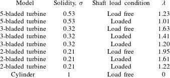
PIV measurements were conducted for the conditions shown in table 1. These conditions corresponded to both load-free (i.e.
 $C_{p}\approx 0$
) and loaded-shaft conditions (i.e.
 $C_{p}>0$
), where the load here refers exclusively to shaft torque, not axial thrust. For the load-free shaft conditions, a comparison was made among the wakes of the four models corresponding to the four model solidities,
 $\unicode[STIX]{x1D70E}$
. For the loaded-shaft conditions, a comparison was made among the wakes of the three turbines while the average rotation rate was held fixed at
 $\unicode[STIX]{x1D706}=1.2$
, and for each turbine while
 $\unicode[STIX]{x1D706}$
was varied.
PIV measurement conditions.
2.7 Calculation of wake statistics
The steady characteristics of the wake were evaluated using the time average of the streamwise component of velocity from the PIV measurements, denoted as
 $\overline{U}$
. Wake dynamics was evaluated using spectral analysis and proper orthogonal decomposition (POD) of both the streamwise (
 $x$
) and spanwise (
 $y$
) fluctuating components of the measured velocity, i.e.
 $u^{\prime }$
and
 $v^{\prime }$
, respectively. Phase-averaged vorticity,
 $\unicode[STIX]{x1D714}_{z}$
, was also calculated from the phase-locked velocity measurements.
A sample of the PIV measurement of
 $\overline{U}$
is shown in figure 6. Additionally, a segment of the time series of
 $v^{\prime }$
, the velocity component used in the spectral analysis, is shown in figure 7. This time series was taken from a single point in the flow, indicated in figure 6 by a solid black circle. Also shown in figure 7 is a dotted line, which is a temporal (spline) interpolation of the measured velocity with a uniform vector spacing in time. This interpolation was a necessary step for the spectral and POD analyses, which are more straightforward to implement with a constant sampling rate. The PIV measurements were not equally distributed in time because they were phase locked to the turbine rotation, which fluctuated due to the unsteady hydrodynamic torque. However, a temporal interpolation was possible because the camera trigger signal had a known sample rate of 2500 Hz. Thus, each TTL pulse to the camera indicated the time stamp for the corresponding velocity field.
Contours of
 $\overline{U}/U_{0}$
for the 3-bladed turbine under load-free shaft conditions (
 $\unicode[STIX]{x1D706}=1.63$
); the zero-level contour is drawn in white. Measurements correspond to PIV window 4 (cf. figure 3). The black circle corresponds to the location of the sample time series in figure 7. Coordinate axes are normalized by the rotor diameter,
 $D$
.

Time series segment of the measured (—) and interpolated
 $(\cdots \,)$
values of
 $v^{\prime }/U_{0}$
corresponding to the sample point in figure 6.

The power spectra for the spanwise component of the velocity fluctuations (
 $v^{\prime }$
) were computed via the method of Welch (Reference Welch1967). For a given streamwise location (
 $x$
), the spanwise point (
 $y$
) was selected based on where the root-mean-square (r.m.s.) of the velocity fluctuations was a maximum, thus indicating the most energetic point along the span. In computing the spectra, a rectangular window function was used with 50 % overlap between windows; the frequency resolution was approximately 0.04 Hz.
2.8 Proper orthogonal decomposition
The POD was used to identify the dominant spatial features of the spatio-temporally evolving wake. A thorough review of the method within the context of the analysis and modelling of turbulent flows is given by Berkooz, Holmes & Lumley (Reference Berkooz, Holmes and Lumley1993). The basic concept of POD is to decompose a dataset into a set of orthogonal modes that are optimal in the sense that the error in projecting the data onto a finite number of modes is minimized. In POD, often a small number of modes suffice to describe a large portion of the variance of the data.
Many variants of POD have been used to extract coherent structures in turbulent flows. The most common approach finds a set of spatial, time-invariant POD modes and their time-varying scalar modal coefficients. The modes are given by eigenfunctions of the correlation tensor between observations at different points in space (and different variables), and efficient computation of the modes follows from the method of snapshots (Sirovich Reference Sirovich1987). This method has been applied in recent studies that examine wind turbine wakes (e.g. Andersen, Sørensen & Mikkelsen Reference Andersen, Sørensen and Mikkelsen2013; VerHulst & Meneveau Reference VerHulst and Meneveau2014; Hamilton, Tutkun & Cal Reference Hamilton, Tutkun and Cal2015).
The approach we employ here is ‘frequency-space’ or ‘spectral’ POD (e.g. Picard & Delville Reference Picard and Delville2000). The advantage of the spectral POD approach for our case is that distinct modes associated with disparate frequencies, such as the blade-passing frequency and the wake vortex shedding frequency, can be obtained independent of their potentially disparate energy levels. Relevant to stationary flows, the spectral POD problem seeks an orthonormal basis for velocity fluctuations
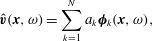 $$\begin{eqnarray}\hat{\boldsymbol{v}}(\boldsymbol{x},\unicode[STIX]{x1D714})=\mathop{\sum }_{k=1}^{N}a_{k}\unicode[STIX]{x1D753}_{k}(\boldsymbol{x},\unicode[STIX]{x1D714}),\end{eqnarray}$$
where
 $\hat{\boldsymbol{v}}$
is the (Fourier transformed in time) two-dimensional velocity fluctuation vector in the plane of the PIV measurements, and the vector POD modes,
 $\unicode[STIX]{x1D753}_{k}$
, are constructed from
 $N$
observations of the vector field
 $\hat{\boldsymbol{v}}^{(k)}(x,\unicode[STIX]{x1D714}),k=1,2,\ldots ,N$
as eigenvectors of
 $$\begin{eqnarray}\int \unicode[STIX]{x1D63E}(\boldsymbol{x},\boldsymbol{x}^{\prime },\unicode[STIX]{x1D714})\unicode[STIX]{x1D753}_{j}(\boldsymbol{x}^{\prime },\unicode[STIX]{x1D714})\,\text{d}\boldsymbol{x}^{\prime }=\unicode[STIX]{x1D706}_{j}(\unicode[STIX]{x1D714})\unicode[STIX]{x1D753}_{j}(\boldsymbol{x},\unicode[STIX]{x1D714}),\quad j=1,2,\ldots ,N,\end{eqnarray}$$
where
 $\unicode[STIX]{x1D63E}$
is the ensemble-averaged cross-spectral density (CSD) tensor
 $$\begin{eqnarray}\unicode[STIX]{x1D63E}(\boldsymbol{x},\boldsymbol{x}^{\prime },\unicode[STIX]{x1D714})=\frac{1}{N}\mathop{\sum }_{k=1}^{N}\hat{\boldsymbol{v}}^{(k)}(\boldsymbol{x},\unicode[STIX]{x1D714})\otimes \hat{\boldsymbol{v}}^{(k)}(\boldsymbol{x}^{\prime },\unicode[STIX]{x1D714}).\end{eqnarray}$$
Note that this tensor involves correlations between each of the two velocity components at each point in space, and every other. The velocity field and volume integral are then discretized on the PIV grid to yield an algebraic eigenvalue problem
 $$\begin{eqnarray}\unicode[STIX]{x1D63E}(\unicode[STIX]{x1D714})\unicode[STIX]{x1D648}\unicode[STIX]{x1D753}(\unicode[STIX]{x1D714})=\unicode[STIX]{x1D706}(\unicode[STIX]{x1D714})\unicode[STIX]{x1D753}(\unicode[STIX]{x1D714}),\end{eqnarray}$$
where the elements of the diagonal matrix,
 $\unicode[STIX]{x1D648}$
are the cell volumes of the PIV grid. The CSD matrix,
 $\unicode[STIX]{x1D63E}$
, may be written
 $\unicode[STIX]{x1D63E}=(1/N)\unicode[STIX]{x1D653}\unicode[STIX]{x1D653}^{H}$
where, for a given frequency,
 $\unicode[STIX]{x1D714}$
,
 $\unicode[STIX]{x1D653}$
is a data matrix whose columns represent the
 $N$
different realizations, and whose rows correspond to each velocity component and each spatial location on the PIV grid (in any convenient ordering). Consideration of the rank of
 $\unicode[STIX]{x1D63E}$
permits one to find the eigenvectors corresponding to non-zero eigenvalues more efficiently by solving the smaller
 $N\times N$
eigenvalue problem
 $(1/N)\unicode[STIX]{x1D653}^{H}\unicode[STIX]{x1D648}\unicode[STIX]{x1D653}\unicode[STIX]{x1D74D}=\unicode[STIX]{x1D706}\unicode[STIX]{x1D74D}$
, and then reconstructing
 $\unicode[STIX]{x1D753}=\unicode[STIX]{x1D653}\unicode[STIX]{x1D74D}$
. Note that the trace of
 $(1/N)\unicode[STIX]{x1D653}^{H}\unicode[STIX]{x1D648}\unicode[STIX]{x1D653}$
is approximately equal to the turbulent kinetic energy (TKE) contained in the frequency bin surrounding
 $\unicode[STIX]{x1D714}$
when integrated over the plane of the PIV measurement.
Numerically, we estimate the CSD matrix using the Welch periodogram method, using the same parameters as were used for the power spectra mentioned in the previous section. Specifically, we generate realizations of the frequency-space velocity field using a rectangular window function on overlapping segments of the time series, and then taking a discrete Fourier transform on each segment with a frequency resolution of approximately 0.04 Hz. The overlap was chosen as 50 %. The eigenvalue problem (2.6) is then solved frequency by frequency using the method discussed above. Approximate independence of the resulting eigenfunctions and eigenvalues was established by varying these parameters of the estimation, within the constraints of the available data.
In the present experiments, the temporal PIV data were collected in different spatial windows in independent experiments. The POD modes must therefore be found independently for each window. If we have reached statistical convergence, then we expect the POD modes (at a given frequency) to match reasonably well near the boundaries of each PIV window, apart from a single complex constant. In what follows, the constant (amplitude and phase) was chosen manually in order to visually align contour plots of the POD modes. The reasonable match we obtain at boundaries of the PIV windows (cf. figure 12) justifies the approach and shows that our modes are indeed reasonably well converged.
3 Results and discussion
3.1 PIV measurements for load-free shaft conditions
Time-averaged PIV measurements of the streamwise component of velocity are shown in figure 8 for the load-free shaft conditions (cf. table 1). The velocity measurements have been normalized by the free stream speed,
 $U_{0}$
, and the coordinate axes by the diameter,
 $D$
. The contour levels are the same in each plot and range in values of
 $\overline{U}/U_{0}$
from
 $-0.3$
to 1.4. Discontinuities in the contours can be observed, mainly at the boundaries of consecutive PIV windows, which are attributable to experimental error. As described in § 2.4, the data collected in each PIV window were a different realization of the same experiment. Between realizations, either the optics or the turbine model was manually moved to a new streamwise location, which introduced a small amount of error in the physical location of the boundary between PIV windows. Additionally, although statistical convergence was checked for the measurement of mean velocity in each PIV window, further error was introduced by variable experimental conditions when different PIV windows were measured on different days. The zero-level contour is shown in white. Within the immediate vicinity of the cylinder and turbine, the large white region in the contour plot is an artefact of shadows created by the model and support structure. However, downstream of the model, this zero-level contour indicates a region of flow recirculation present in each of the four cases shown.
For the cylinder, this recirculation region is attached to the points of separation from the surface of the model. For the 3- and 5-bladed turbine, the recirculation region is qualitatively similar to that of the cylinder, but is detached from the model and is angled toward the negative y-axis due to the turbine rotation. There is also a recirculation region present in the wake of the 2-bladed turbine, but it is distinct in form to that of the other models, extending from approximately tangent to the blade path to just beyond
 $2D$
downstream of the turbine centre. The presence of a recirculation region in the wake of each of the turbine models was found to be a function of
 $\unicode[STIX]{x1D706}$
, with decreasing
 $\unicode[STIX]{x1D706}$
causing the region to change in size and in some cases disappear completely. This trend can be readily observed in comparing the contour plots of the current section with those of the remaining cases given in figure 29 of the appendix. In all cases, there is a notable asymmetry of the VAWT wake. This is attributed to the stronger shear layer that forms on the side of the turbine where the blades are advancing upstream. A surprising result, however, is that the deficit in the wake velocity recovers faster with increasing model solidity (
 $\unicode[STIX]{x1D70E}$
), with the fastest recovery achieved by the stationary cylinder; there is also a broader wake with decreasing solidity.
Contours of
 $\overline{U}/U_{0}$
measured under load-free shaft conditions for the (a) 2-bladed VAWT, (b) 3-bladed VAWT, (c) 5-bladed VAWT and (d) cylinder. Airfoil cross-sections for the turbines are drawn to scale.

It is important to emphasize that the turbine cases shown in figure 8 were for a turbine free to rotate without an external torque applied to its shaft, i.e.
 $C_{p}\approx 0$
. From momentum theory (e.g. Hau Reference Hau2005), the turbine power coefficient is given as
 $C_{p}=4a(1-a)^{2}$
, where
 $a$
is the axial induction factor, defined as
 $a\equiv 1-U_{r}/U_{0}$
, where
 $U_{r}$
is the speed of the flow at the rotor. Similarly, the turbine thrust coefficient,
 $C_{T}$
, is given as
 $C_{T}=4a(1-a)$
. This implies that as
 $C_{p}$
tends toward zero (with increasing
 $\unicode[STIX]{x1D706}$
), as in figure 8, the induction factor tends toward 1 and
 $C_{T}$
tends toward zero. Empirically, the thrust coefficient does not follow momentum theory for large induction factor (
 $a>0.5$
), but rather increases above 1 for large
 $a$
in HAWT wakes (e.g. Buhl Reference Buhl2005; Leishman Reference Leishman2006; Hansen Reference Hansen2008). This suggests that the measurements shown in figure 8 are for a rotor with large axial thrust and implies a ‘turbulent wake state’ (e.g. Eggleston & Stoddard Reference Eggleston and Stoddard1987).
Figure 9 shows the velocity power spectra computed at five different streamwise locations for each of the cases shown in figure 8. The frequency along the abscissa in these plots has been normalized to give the standard definition of the Strouhal number for cylinder vortex shedding, i.e.
 $St=fD/U_{0}$
. In the case of the cylinder (cf. figure 9
d), the streamwise evolution of the spectra shows a dominant peak near
 $St\approx 0.2$
that forms and eventually decays with downstream distance, in agreement with existing literature (e.g. Roshko Reference Roshko1961). For the turbines, however, there is a bi-modal behaviour in the evolution of the velocity spectra with downstream distance. In the near-wake region of the turbine, there is a sharp spectral peak that corresponds to the blade-passing frequency. This is consistent with previous investigations of the near-wake region of a VAWT, which has been shown to be dominated by blade–vortex dynamics (see, e.g. Tescione et al.
Reference Tescione, Ragni, He, Ferreira and van Bussel2014; Bachant & Wosnik Reference Bachant and Wosnik2015). Further downstream, however, the spectra reveal a transition that occurs in the wake, where the dominant velocity fluctuations shift to a lower frequency of
 $St\approx 0.26$
, roughly independent of the blade-passing frequency. Additionally, at its maximum, the amplitude of the far-wake peak reaches very near to that of the near-wake peak, which suggests that there is a dynamic shift in the energy content of the flow before much of it can be lost to viscous dissipation.
Single-point spectra of the velocity fluctuations (
 $v^{\prime }$
) taken at
 $X/D=0.9$
(——),
 $X/D=1.7$
(– – –),
 $X/D=3.3$
(– - – -),
 $X/D=7.3$
(- - - - -), and
 $X/D=10.0$
(
 $\cdots \cdots$
). The spectra correspond to load-free shaft conditions for the (a) 2-bladed VAWT, (b) 3-bladed VAWT, (c) 5-bladed VAWT and (d) cylinder. Dotted vertical lines correspond to the selected near- and far-wake frequencies of the maximum amplitude in the spectra.

An analysis of the dominant POD mode illustrates the spatio-temporal variation of the velocity fluctuations in the wake. Figure 10 shows the power spectral density of the amplitude of the dominant POD mode across a range of frequencies for the cases shown in figure 8. This approach to the POD analysis was described in § 2.7. Each spectrum corresponds to one of the PIV windows. In comparing the local and global spectra of figures 9 and 10, respectively, it appears that the dominant POD mode captures the bluff-body oscillations of the cylinder wake and the bi-modal oscillations present in the VAWT wake. Figure 11 shows a comparison of the phase-averaged vorticity field with contours of the dominant POD mode at the blade-passing frequency for each of the three turbines. Since the angular position of the turbine blades in each case is accurately represented in the figure, the vortex structures that are clearly present in the phase-averaged vorticity contours offer a direct interpretation of the structures present in the contours of the spatial mode. More specifically, a pair of positive (red) and negative (blue) structures in the spatial mode contour is representative of the spatial extent of a coherent vortex structure in the turbine wake. The purpose of including figure 11 is to emphasize that the coherent structures that we observe from the contours of the dominant POD mode at a given frequency can be interpreted directly as coherent vortices in the flow, which is not always a result of the POD analysis (Kostas, Soria & Chong Reference Kostas, Soria and Chong2005).
Spectra of the amplitude of the dominant POD mode for the velocity fluctuations under load-free shaft conditions for the (a) 2-bladed VAWT, (b) 3-bladed VAWT, (c) 5-bladed VAWT and (d) cylinder. The spectra correspond to PIV window 3 (○), 4 (
 $\times$
), 5 (+), 6 (*), 7 (▫), 8 (♢) and 9 (▿). Dotted vertical lines correspond to the selected near- and far-wake frequencies of the maximum amplitude in the spectra.

(a,c,e) Contours of the phase-averaged vorticity for the (a) 2-bladed VAWT, (c) 3-bladed VAWT and (e) 5-bladed VAWT. (b,d,f) Contours of the spanwise component (
 $v^{\prime }$
) of the dominant POD mode for the velocity fluctuations at the blade-passing frequency for the (b) 2-bladed VAWT, (d) 3-bladed VAWT and (f) 5-bladed VAWT. Airfoil cross-sections and angular positions are accurately represented in the figure. The dashed circle in each plot is for reference and corresponds to the turbine diameter.

Figures 12 and 13 show contours of the spanwise (
 $v^{\prime }$
) and streamwise (
 $u^{\prime }$
) components of the dominant POD mode at the far-wake peak frequency (cf. figure 10), respectively, for the same flow conditions as before. There is a strong resemblance between the spatial mode structure in far wake of the VAWT to that of the cylinder, especially as the turbine solidity (
 $\unicode[STIX]{x1D70E}$
) is increased. The structure of the cylinder mode is consistent with what has been previously reported (see, e.g. Feng, Wang & Pan Reference Feng, Wang and Pan2011), and the alternating pattern of vortices shed from the cylinder can again be inferred by the pairs of structures within the spatial mode contour, i.e. a single vortex structure is represented by two spatial mode structures with alternating sign. This implies that the far wake of the VAWT is characterized by large-scale structures that are typically periodic in both space and time and alternate in sign, akin to a bluff body. This bluff-body mode tends to be stronger in amplitude on the windward side of the turbine, i.e. where the stronger shear layer is formed, indicating that it is likely caused by an underlying shear-layer instability. It also appears as though the development of these far-wake structures in the VAWT wake is delayed downstream as the turbine solidity is reduced. However, in these load-free shaft conditions, the rotation rate of the turbine was uncontrolled, which adds an additional variable to consider in the analysis. These variables are decoupled in the following section.
Contours of the spanwise component (
 $v^{\prime }$
) of the dominant POD mode for the velocity fluctuations at the far-wake peak frequency (cf. figure 10) for the (a) 2-bladed VAWT, (b) 3-bladed VAWT, (c) 5-bladed VAWT (d) and cylinder. Airfoil cross-sections and angular positions are accurately represented in the figure. The dashed circle in the turbine plots is for reference only and corresponds to the turbine diameter. The solid circle represents the cylinder diameter,
 $D$
.

Contours of the streamwise component (
 $u^{\prime }$
) of the dominant POD mode for the velocity fluctuations at the far-wake peak frequency (cf. figure 10) for the (a) 2-bladed VAWT, (b) 3-bladed VAWT, (c) 5-bladed VAWT (d) and cylinder. Airfoil cross-sections and angular positions are accurately represented in the figure. The dashed circle in the turbine plots is for reference only and corresponds to the turbine diameter. The solid circle represents the cylinder diameter,
 $D$
.

Contours of the spanwise component (
 $v^{\prime }$
) of the dominant POD mode for the velocity fluctuations at both the near- and far-wake peak frequencies (cf. figure 10) for the (a) 2-bladed VAWT, (b) 3-bladed VAWT and (c) 5-bladed VAWT. In each case,
 $\unicode[STIX]{x1D706}$
 ${\approx}1.2$
. Airfoil cross-sections and angular positions are accurately represented in the figure. The dashed circle in the turbine plots is for reference only and corresponds to the turbine diameter.

3.2 PIV measurements for loaded-shaft conditions
To separate the effects of increasing the turbine solidity from varying its rotation, both were evaluated independently. The same procedure was followed as before, but only the results of the POD mode analysis are presented here; the corresponding spectra are given in figure 30 of the appendix. Figure 14 shows contours of the spanwise velocity component of the dominant POD mode while
 $\unicode[STIX]{x1D706}$
was held fixed and
 $\unicode[STIX]{x1D70E}$
was varied. Note that in this figure the dominant mode at two distinct frequencies have been superposed together, i.e. the dominant frequency in the near and far wake. The combination of these two temporal frequencies gives a broad look at the dominant spatial structure of the evolving wake. Immediately apparent from figure 14 is that increasing
 $\unicode[STIX]{x1D70E}$
leads to an earlier transition to bluff-body oscillations in the VAWT wake. Also apparent, is that as
 $\unicode[STIX]{x1D70E}$
is decreased, there is a sharp increase in the strength of the vortices that are shed from the blades, which can be deduced from the larger amplitude and spatial extent of the mode structure.
Contours of the spanwise component (
 $v^{\prime }$
) of the dominant POD mode for the velocity fluctuations at both the near- and far-wake peak frequencies (cf. figure 10). The contours plots correspond to the 3-bladed VAWT with an average rotation rate of (a)
 $\unicode[STIX]{x1D706}=1.20$
, (b)
 $\unicode[STIX]{x1D706}=1.41$
and (c)
 $\unicode[STIX]{x1D706}=1.63$
. Airfoil cross-sections and angular positions are accurately represented in the figure. The dashed circle in the turbine plots is for reference only and corresponds to the turbine diameter.

Figure 15 shows contours of the spanwise velocity component of the dominant POD mode for the 3-bladed turbine while its rotation rate was varied from
 $\unicode[STIX]{x1D706}\approx 1.2$
–1.6. As before, the dominant mode at the near- and far-wake peak frequency have been superposed together. Despite the small range of
 $\unicode[STIX]{x1D706}$
, a similar shift in transition is observed among these cases as was when varying the solidity, with the transition occurring closer to the turbine with increasing
 $\unicode[STIX]{x1D706}$
. This suggests the concept of an apparent solidity for the turbine due to both its geometric solidity as well as its rotation rate, which we derive in the following section.
3.3 Dynamic solidity of a VAWT
The effects of geometric solidity and rotation rate can be combined using the concept of a ‘dynamic solidity’. In the limit of
 $\unicode[STIX]{x1D706}\gg 1$
, there is little time for the incident flow to react to the passage of the turbine blades, resulting in the turbine rotor appearing to the flow as like a solid cylinder. Conversely, when
 $\unicode[STIX]{x1D706}=0$
, the interaction of the incident flow with the turbine blades is indeterminate, since it depends on the orientation of the rotor. However, for a given orientation, a larger geometric solidity (
 $\unicode[STIX]{x1D70E}$
) means that the turbine rotor approaches the geometry of a cylinder, and thus would interact with the flow accordingly.
One way to quantify these limits is to formulate a dynamic solidity parameter,
 $\unicode[STIX]{x1D70E}_{D}$
, using the characteristic scales of the flow. We first define a characteristic length scale,
 $l$
, as the sum of the gaps in the circumference of the turbine rotor, i.e.
 $l=\unicode[STIX]{x03C0}D(1-\unicode[STIX]{x1D70E})$
. Using this, we define a VAWT time scale,
 $t_{V}$
, as
 $$\begin{eqnarray}t_{V}=\frac{l}{nU_{0}\unicode[STIX]{x1D706}},\end{eqnarray}$$
where
 $n$
is the number of blades. This represents the time required for the turbine blades to collectively sweep through the distance to close the gaps between the blades. Next, we define a convective time scale,
 $t_{conv}=l/U_{0}$
, which represents the amount of time required for a free stream fluid particle to travel the same distance. The ratio
 $t_{V}/t_{conv}$
represents the percentage of convection time required to close the gaps between the blades, with a smaller percentage resulting in the turbine appearing more solid to the incident flow. We multiply this ratio of time scales by a geometric factor,
 $R/c$
, where
 $R$
is the turbine radius and
 $c$
is the chord length, to incorporate the rotor geometry, and subtract this quantity from unity to give the definition of dynamic solidity as
 $$\begin{eqnarray}\unicode[STIX]{x1D70E}_{D}=1-\frac{R}{c}\frac{t_{V}}{t_{conv}}=1-\frac{1}{2\unicode[STIX]{x03C0}\unicode[STIX]{x1D70E}\unicode[STIX]{x1D706}}.\end{eqnarray}$$
Note that this definition follows the aforementioned limiting behaviours. For a given rotor geometry and
 $\unicode[STIX]{x1D706}\gg 1$
,
 $\unicode[STIX]{x1D70E}_{D}\approx 1$
, corresponding to the geometric solidity of a solid cylinder (
 $\unicode[STIX]{x1D70E}=1$
). When
 $\unicode[STIX]{x1D706}=0$
,
 $\unicode[STIX]{x1D70E}_{D}$
is indeterminate. Similarly, if
 $\unicode[STIX]{x1D706}<1/2\unicode[STIX]{x03C0}\unicode[STIX]{x1D70E}$
, which is practically insignificant, then
 $\unicode[STIX]{x1D70E}_{D}<0$
, which loses physical meaning. However, for
 $\unicode[STIX]{x1D706}>1/2\unicode[STIX]{x03C0}\unicode[STIX]{x1D70E}$
,
 $\unicode[STIX]{x1D70E}_{D}$
increases monotonically with increasing either
 $\unicode[STIX]{x1D70E}$
or
 $\unicode[STIX]{x1D706}$
. Figure 16 shows how
 $\unicode[STIX]{x1D70E}_{D}$
varies with
 $\unicode[STIX]{x1D706}$
and
 $\unicode[STIX]{x1D70E}$
for a turbine with fixed chord length (
 $c=0.1~\text{m}$
) and rotor diameter (
 $D=0.3~\text{m}$
), as in the present experiment. Also shown in the figure are the conditions measured during the experiment, indicated by symbols. The relation between
 $\unicode[STIX]{x1D70E}_{D}$
and the transition to bluff-body dynamics in the VAWT wake is explored in the next section.
Dynamic solidity,
 $\unicode[STIX]{x1D70E}_{D}$
, variation with
 $\unicode[STIX]{x1D706}$
and
 $\unicode[STIX]{x1D70E}$
. Measured values are shown with colours and symbols that correspond to the following: the 2-bladed turbine for
 $\unicode[STIX]{x1D706}=1.95$
(
 $\times$
), 1.61 (▫ (blue)) and 1.22 (○ (blue)), the 3-bladed turbine for
 $\unicode[STIX]{x1D706}=1.63$
(▫ (black)), 1.41 (▵) and 1.20 (○ (black)), the 5-bladed turbine for
 $\unicode[STIX]{x1D706}=1.23$
(○ (red)) and
 $\unicode[STIX]{x1D706}=1.01$
(
 $+$
).

Normalized frequency of the maximum amplitude in the velocity spectra,
 $St_{max}$
. Colours and symbols correspond to the following: the 2-bladed turbine for
 $\unicode[STIX]{x1D706}=1.95$
(
 $\times$
), 1.61 (▫ (blue)) and 1.22 (○ (blue)), the 3-bladed turbine for
 $\unicode[STIX]{x1D706}=1.63$
(▫ (black)), 1.41 (▵) and 1.20 (○ (black)), the 5-bladed turbine for
 $\unicode[STIX]{x1D706}=1.23$
(○ (red)) and
 $\unicode[STIX]{x1D706}=1.01$
(
 $+$
) and the stationary cylinder (●). Downstream distance,
 $X$
, is normalized by the model diameter,
 $D$
. The horizontal dashed line corresponds to
 $St_{max}=0.2$
. Vertical dashed lines correspond to the location of the streamwise transition points in each case, i.e.
 $(X/D)_{transition}$
.

3.4 Effect of dynamic solidity on wake transition
Figure 17 shows a plot of Strouhal number versus normalized downstream distance for all of the cases shown in figure 16 with the addition of the stationary cylinder measurements. Each point in figure 17 indicates the non-dimensional frequency of the maximum amplitude in a single velocity spectrum, denoted as
 $St_{max}$
. Each spectrum was computed at a single point in the flow where the r.m.s. of the spanwise velocity fluctuations was a maximum. This is a convenient way to express all of the data at once, and it illustrates what has already been shown for a few cases, e.g. the bi-modal behaviour of the VAWT wake. As the near-wake vortices decay, the transition to bluff-body oscillations in the far wake is indicated in figure 17 by the collapse of the data toward
 $St=0.2$
, indicated by the horizontal dashed line. The start of the wake transition in each case is located at
 $(X/D)_{transition}$
, indicated by vertical dashed lines in the figure. Each
 $(X/D)_{transition}$
location is given by the furthest downstream point where the frequency of the dominant spanwise velocity fluctuations is equal to the blade-passing frequency. Further downstream of this point, there was consistently a sharp decrease in the frequency of the dominant velocity fluctuations. Physically, this means that
 $(X/D)_{transition}$
marks the streamwise point in the flow where the blade vortices have decayed to the point where they no longer account for the most energetic fluctuations in the flow and a transition to bluff-body oscillations begins to dominate the wake dynamics. The scatter of the data in the far wake is due in part to the spectral resolution, which was
 $St\approx \pm 0.05$
for all cases, limited by the sample size. Additionally, the slight increase away from
 $St=0.2$
is speculated to be an effect of the VAWT’s rotation. In rotating cylinder experiments, Lam (Reference Lam2009) observed an increase in the vortex shedding frequency from
 $St=0.18$
to 0.29 as the cylinder’s rotation was increased from
 $\unicode[STIX]{x1D706}=0$
to 1.68.
Linear correlation (
 $R^{2}=0.94$
) between the streamwise location of wake transition, i.e.
 $(X/D)_{transition}$
, and dynamic solidity,
 $\unicode[STIX]{x1D70E}_{D}$
.

It was found that there exists a strong correlation between the dynamic solidity,
 $\unicode[STIX]{x1D70E}_{D}$
, and the downstream transition location,
 $(X/D)_{transition}$
, deduced from figure 17. Figure 18 shows this correlation along with a linear regression fit to the data points. Note that the transition location for the cylinder is defined to be
 $(X/D)_{transition}\equiv 0$
, which can be thought of as a transition to bluff-body oscillations that immediately dominates the wake dynamics. The linear regression of figure 18 is referred to in subsequent sections and is given as the following:
 $$\begin{eqnarray}(X/D)_{transition}=4.78-4.93\unicode[STIX]{x1D70E}_{D}.\end{eqnarray}$$
When the abscissa of each case in figure 17 is normalized by
 $(X/D)_{transition}$
, given by (3.3), and the ordinate axis by the non-dimensional blade-passing frequency in each case,
 $St_{blade}$
, defined as
 $$\begin{eqnarray}St_{blade}=\frac{f_{blade}D}{U_{0}}=\left(\frac{nU_{0}\unicode[STIX]{x1D706}}{\unicode[STIX]{x03C0}D}\right)\frac{D}{U_{0}}=\frac{n\unicode[STIX]{x1D706}}{\unicode[STIX]{x03C0}},\end{eqnarray}$$
the result is a collapse of the data in the near wake and alignment of the start of far-wake transition. This is shown in figure 19. The implication of this finding is that the downstream distance at which point the VAWT wake begins to transition to a state dominated by bluff-body dynamics, i.e.
 $X_{transition}$
, can be predicted using a simple relation between the turbine geometry and its kinematics, which can be explicitly written as the following:
 $$\begin{eqnarray}X_{transition}=D(4.78-4.93\unicode[STIX]{x1D70E}_{D}).\end{eqnarray}$$
Ratio of
 $St_{max}$
to the normalized blade-passing frequency,
 $St_{blade}$
. Colours and symbols correspond to the following: the 2-bladed turbine for
 $\unicode[STIX]{x1D706}=1.95$
(
 $\times$
), 1.61 (▫ (blue)) and 1.22 (○ (blue)), the 3-bladed turbine for
 $\unicode[STIX]{x1D706}=1.63$
(▫ (black)), 1.41 (▵) and 1.20 (○ (black)) and the 5-bladed turbine for
 $\unicode[STIX]{x1D706}=1.23$
(○ (red)) and
 $\unicode[STIX]{x1D706}=1.01$
(
 $+$
). Downstream distance,
 $X$
, is normalized by
 $X_{transition}$
given by (3.5). The vertical dashed line corresponds to
 $X/X_{transition}=1$
, the streamwise transition location in the VAWT wake.

3.5 Effect of dynamic solidity on velocity recovery
Until now, the discussion has focused mainly on the behaviour of the wake dynamics. This section will further explore how this behaviour relates to the recovery of the wake velocity deficit. For a given streamwise location, the minimum velocity was found by taking the minimum across the span (neglecting measurement points near the walls). Figure 20 shows the time average of the minimum streamwise component of velocity,
 $\overline{U}_{min}$
, measured for the cases corresponding to figure 17. Upon examining figure 20, it can be observed that the velocity deficit and its subsequent recovery happen in a similar manner for all cases. However, the recovery occurs at a different rate initially in each case, indicated by the slopes of the curves. Additionally, we can compare the absolute minimum of the streamwise component of velocity in the wake, taken to be the minimum of the velocity profiles shown in figure 20. Figure 21 shows a plot of this absolute minimum velocity versus the dynamic solidity in each case. There is again a significant correlation between these two variables. Physically, this is consistent with the idea that the more solid the turbine appears to the incoming flow, the greater is the initial velocity deficit in the wake.
Minimum streamwise velocity across the span,
 $\overline{U}_{min}$
. Colours and symbols correspond to the following: the 2-bladed turbine for
 $\unicode[STIX]{x1D706}=1.95$
(
 $\times$
), 1.61 (▫ (blue)) and 1.22 (○ (blue)), the 3-bladed turbine for
 $\unicode[STIX]{x1D706}=1.63$
(▫ (black)), 1.41 (▵) and 1.20 (○ (black)), the 5-bladed turbine for
 $\unicode[STIX]{x1D706}=1.23$
(○ (red)) and
 $\unicode[STIX]{x1D706}=1.01$
(
 $+$
) and the stationary cylinder (●). Downstream distance,
 $X$
, is normalized by the model diameter,
 $D$
, and velocity by the free stream speed,
 $U_{0}$
.

Linear correlation (
 $R^{2}=0.96$
) between the normalized absolute minimum streamwise velocity across the span,
 $\min (\overline{U}_{min}/U_{0})$
and the dynamic solidity,
 $\unicode[STIX]{x1D70E}_{D}$
.

To compare the rate of recovery of the velocity deficit, we first rescale the ordinate axis of figure 20 by the absolute minimum velocity, min(
 $\overline{U}_{min}$
), such that all of the curves have the same initial deficit, shown in figure 22. If we then assume that the recovery rate reaches an equilibrium in all cases by 12
 $D$
downstream of the turbine centre (i.e. the furthest downstream measurement point) and plot this rescaled velocity against dynamic solidity, the result is shown in figure 23. The strong correlation between the final rescaled minimum velocity and the dynamic solidity indicates that increasing the dynamic solidity results in a faster rate of recovery of the velocity deficit in the wake.
Minimum streamwise velocity,
 $\overline{U}_{min}$
, rescaled by the absolute minimum velocity across the span, i.e. min(
 $\overline{U}_{min}$
). Colours and symbols correspond to the following: the 2-bladed turbine for
 $\unicode[STIX]{x1D706}=1.95$
(
 $\times$
), 1.61 (▫ (blue)) and 1.22 (○ (blue)), the 3-bladed turbine for
 $\unicode[STIX]{x1D706}=1.63$
(▫ (black)), 1.41(▵) and 1.20 (○ (black)), the 5-bladed turbine for
 $\unicode[STIX]{x1D706}=1.23$
(○ (red)) and
 $\unicode[STIX]{x1D706}=1.01$
(
 $+$
) and the stationary cylinder (●). Downstream distance
 $X$
is normalized by the model diameter,
 $D$
, and velocity by the free stream speed,
 $U_{0}$
.

Linear correlation (
 $R^{2}=0.99$
) between the rescaled streamwise velocity of figure 22 at
 $X/D=12$
and the dynamic solidity,
 $\unicode[STIX]{x1D70E}_{D}$
.

Since there is a strong correlation between the recovery of the velocity deficit and the dynamic solidity, we can rescale the abscissa of the velocity curves by the
 $(X/D)_{transition}$
location as was done before in figure 19. The result of this transformation on the measured minimum velocity (cf. figure 20) is shown in figure 24. Notably, all of the velocity profiles recover at approximately the same rate, indicated qualitatively by their slope. However, the transformation is incomplete since the ordinate axis was not scaled. Additionally, the imperfect scaling of the abscissa is attributable to the imperfect means used to predict the transition location, i.e. equation (3.5). Most important, however, is that the collapse of the velocity profiles in the transformed coordinate suggests that the bluff-body mode is instrumental in the recovery of the velocity deficit, perhaps because it controls the entrainment of energy into the wake.
Normalized minimum streamwise velocity,
 $\overline{U}_{min}/U_{0}$
, versus downstream distance
 $X$
normalized by the streamwise transition location,
 $X_{transition}$
. Colours and symbols correspond to the following: the 2-bladed turbine for
 $\unicode[STIX]{x1D706}=1.95$
(
 $\times$
), 1.61 (▫ (blue)) and 1.22 (○ (blue)), the 3-bladed turbine for
 $\unicode[STIX]{x1D706}=1.63$
(▫ (black)), 1.41(▵) and 1.20 (○ (black)) and the 5-bladed turbine for
 $\unicode[STIX]{x1D706}=1.23$
(○ (red)) and
 $\unicode[STIX]{x1D706}=1.01$
(
 $+$
).

Furthermore, the collapse suggests the possibility of extracting an equation relating the minimum velocity,
 $\overline{U}_{min}/U_{0}$
, to the
 $X/X_{transition}$
position in the wake. This is explored first within the context of classical theory of turbulent free-shear flows, then subsequently compared with previous wind turbine wake studies. Invoking Prandtl’s mixing length hypothesis, Schlichting (Reference Schlichting1960) derived an expression for the recovery of the centreline velocity deficit, i.e. the minimum, in the wake of a bluff body. For a two-dimensional wake, this is given as:
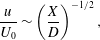 $$\begin{eqnarray}\frac{u}{U_{0}}\sim \left(\frac{X}{D}\right)^{-1/2},\end{eqnarray}$$
and for a circular wake (i.e. 3-D axisymmetric), as:
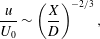 $$\begin{eqnarray}\frac{u}{U_{0}}\sim \left(\frac{X}{D}\right)^{-2/3},\end{eqnarray}$$
where
 $u=U_{0}-\overline{U}_{min}$
. Assuming that the maximum velocity deficit in the wake of the VAWT follows the above form, we seek solutions to the following equation:
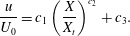 $$\begin{eqnarray}\frac{u}{U_{0}}=c_{1}\left(\frac{X}{X_{t}}\right)^{c_{2}}+c_{3}.\end{eqnarray}$$
The coefficients for this power law fit in each case are given in table 2. Note that the curves were fit to the measured data downstream of the absolute minimum velocity for each case. A curve fit to the cylinder data is also included, but this was done without applying a transformation to its abscissa, since by definition the transition occurs immediately at
 $X/D=0$
. In general, the power law appears to be an excellent fit to the measured VAWT data in the transformed coordinate, with an
 $R^{2}\sim 0.99$
in all cases. This power law trend can also be readily observed in figure 25, where the measured velocity deficit in the VAWT wake, i.e.
 $u/U_{0}=1-(\overline{U}_{min}/U_{0})$
, has been plot on a log–log scale. These observations are also consistent with several earlier HAWT wake studies where a power law was used to describe the downstream evolution of the wake velocity deficit (e.g. Högström et al.
Reference Högström, Asimakopoulos, Kambezidis, Helmist and Smedman1988; Vermeer, Sørensen & Crespo Reference Vermeer, Sørensen and Crespo2003; Zhang, Markfort & Porté-Agel Reference Zhang, Markfort and Porté-Agel2013; Iungo & Porté-Agel Reference Iungo and Porté-Agel2014). The typical form of this power law for HAWT wakes is given in Iungo & Porté-Agel (Reference Iungo and Porté-Agel2014) as the following:
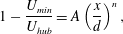 $$\begin{eqnarray}1-\frac{U_{min}}{U_{hub}}=A\left(\frac{x}{d}\right)^{n},\end{eqnarray}$$
where
 $U_{hub}$
is a reference velocity,
 $U_{min}$
is the minimum axial velocity observed at a certain downstream distance,
 $(x/d)$
is the downstream distance normalized by the rotor diameter,
 $A$
is a constant related to the turbine thrust coefficient and
 $n$
is related to the rate of wake recovery. The typical values for the coefficients are also given as
 $1<A<3$
and
 $-1.25<n<-0.25$
, which are within the range of values of coefficients
 $c_{1}$
and
 $c_{2}$
in table 2, respectively, despite that the latter were obtained for the VAWT and cylinder wakes. This further suggests a commonality among the different wake flows.
Log–log plot of normalized velocity deficit,
 $u/U_{0}=1-(\overline{U}_{min}/U_{0})$
, versus downstream distance
 $X$
normalized by the streamwise transition location,
 $X_{transition}$
. Colours and symbols correspond to the following: the 2-bladed turbine for
 $\unicode[STIX]{x1D706}=1.95$
(
 $\times$
), 1.61 (▫ (blue)) and 1.22 (○ (blue)), the 3-bladed turbine for
 $\unicode[STIX]{x1D706}=1.63$
(▫ (black)), 1.41 (▵) and 1.20 (○ (black)) and the 5-bladed turbine for
 $\unicode[STIX]{x1D706}=1.23$
(○ (red)) and
 $\unicode[STIX]{x1D706}=1.01$
(
 $+$
). Two dotted lines are drawn for reference, one with a
 $-1$
slope and another with a
 $-2/3$
slope.

Power law coefficients corresponding to (3.8).
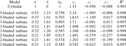
Additionally, the variation of the exponent,
 $c_{2}$
in table 2, indicates the importance of considering the three-dimensionality of the flow, especially with increasing dynamic solidity. For
 $\unicode[STIX]{x1D70E}_{D}<0.65$
, the minimum velocity in the wake increases approximately in proportion to
 $X^{-0.6}$
, which could perhaps be approximated by the previous theoretical expressions. For
 $\unicode[STIX]{x1D70E}_{D}>0.65$
, the minimum velocity in the wake increases approximately in proportion to
 $X^{-1}$
, including for the cylinder. This indicates that for small aspect ratio and large dynamic solidity, neither 2-D nor 3-D-axisymmetric assumptions are valid in the VAWT wake. This is physically consistent with the idea that the finite aspect ratio of the models plays an increasingly dominant role in the wake recovery as the dynamic solidity increases. Furthermore, the variation of
 $c_{2}$
is likely affected by all phenomena that can affect the wake Reynolds stresses, e.g. the free stream turbulence intensity, since these stresses influence the wake recovery rate. To this end, the effect of the three-dimensionality of the flow, including an evaluation of the Reynolds stresses, is explored further in § 3.6.
All of the measured values, including the cylinder data, are plotted in figure 26 with a proposed scaling of the ordinate axis. This rescaling includes subtracting the absolute minimum velocity in each case, min(
 $\overline{U}_{min}$
), as well as normalizing by the total velocity deficit. Upon examining figure 26, the closeness of the cylinder data to that of the transformed VAWT data offers another interpretation to this coordinate transformation, which is a mapping of the minimum deficit in the VAWT wake onto that of the cylinder. This suggests that a simplified approach to approximate the wake of a VAWT of arbitrary dynamic solidity could be achieved by applying the inverse transformation to the wake of a stationary cylinder. Although this would not account for effects such as wake asymmetry, it could give a first-order approximation for the velocity deficit recovery.
Minimum streamwise velocity,
 $\overline{U}_{min}$
, rescaled by the absolute minimum streamwise velocity across the span, min(
 $\overline{U}_{min}$
). Downstream distance
 $X$
is normalized by the streamwise transition location,
 $X_{transition}$
, for the turbine data and
 $D$
for the cylinder. Colours and symbols correspond to the following: the 2-bladed turbine for
 $\unicode[STIX]{x1D706}=1.95$
(
 $\times$
), 1.61 (▫ (blue)) and 1.22 (○ (blue)), the 3-bladed turbine for
 $\unicode[STIX]{x1D706}=1.63$
(▫ (black)), 1.41 (▵) and 1.20 (○ (black)) the 5-bladed turbine for
 $\unicode[STIX]{x1D706}=1.23$
(○ (red)) and
 $\unicode[STIX]{x1D706}=1.01$
(
 $+$
) and the stationary cylinder (●).

3.6 Insight into three-dimensional effects
Thus far, the analysis has focused exclusively on the 2-D PIV measurements. Next we examine the out-of-plane (
 $XZ$
) PIV measurements to provide insight into the three-dimensionality of the flow, which was suggested in the last section to be significant for high dynamic solidity cases.
Figure 27 shows time-averaged PIV measurements of the streamwise and vertical components of velocity,
 $\overline{U}$
and
 $\overline{W}$
, respectively, for each of the previous experimental cases. These measurements corresponded to a single streamwise position,
 $X/D=3.8$
, which was located in the middle of the field of view of the
 $XZ$
-PIV measurements. Also shown for comparison in each plot are measurements of the free stream velocity, taken at the same
 $X/D$
location, but with the model removed. A fully developed turbulent boundary layer profile is observed from these free stream measurements. Near the top of the measurement window, there is a slight distortion to the boundary layer profile as the flow tries to adjust to the Plexiglas sheet used to dampen free-surface effects. This effect on the boundary layer profile is negligible given its limited spatial extent.
Time-averaged PIV measurements of streamwise,
 $\overline{U}$
(left column), and vertical,
 $\overline{W}$
(right column), velocity components at
 $X/D=3.75$
. Measurements are shown along the
 $Z$
-axis, normalized by the height of the rotor,
 $H$
, where
 $Z/H=0.64$
is at the rotor midspan. The free stream measurements are indicated by solid black circles in each plot. Data in each panel correspond to the following: (a,b) the 2-bladed turbine for
 $\unicode[STIX]{x1D706}=1.95$
(
 $\times$
), 1.61 (▫ (blue)) and 1.22 (○ (blue)); (c,d) the 3-bladed turbine for
 $\unicode[STIX]{x1D706}=1.63$
(▫ (black)), 1.41 (▵) and 1.20 (○ (black)); (e,f) the stationary cylinder (●) and the 5-bladed turbine for
 $\unicode[STIX]{x1D706}=1.23$
(○ (red)) and
 $\unicode[STIX]{x1D706}=1.01$
(
 $+$
).

Qualitatively, the flow appears nearly symmetric about the midspan for all cases, but with a significant variation of the streamwise velocity along the
 $Z$
-axis. Despite the large variation in
 $\overline{U}$
along the height, ranging from approximately 0 to 0.6
 $U_{0}$
, the average vertical velocity never exceeds about 0.07
 $U_{0}$
. This suggests at least two possibilities that may occur in the experiment related to three-dimensional wake effects. The first is that 3-D effects may have dissipated by this downstream position, such that the flow may be reasonably represented by two-dimensional slices at different heights. The second is that since the turbine almost completely fills the height of the channel, the limited space above and below the turbine may have a similar effect on the flow as using end-plates, which tend to suppress three-dimensional effects.
It is interesting to note that the cylinder velocity profile, shown in figure 27(e,f) along with the 5-bladed turbine, appears to recover faster than all the other cases, which is consistent with the previous wake recovery analysis. An important question left to answer, however, is how the Reynolds stresses compare in the different measurement planes, since this is more telling of which direction provides more of a contribution to the wake recovery. The Reynolds stresses, i.e.
 $\langle u^{\prime }v^{\prime }\rangle$
and
 $\langle u^{\prime }w^{\prime }\rangle$
, at the same
 $X/D$
location are shown in figure 28 for the cases shown in figure 27. Notable from these figures is that the vertical shear stress, i.e.
 $\langle u^{\prime }w^{\prime }\rangle$
, is approximately the same order as the spanwise shear stress, i.e.
 $\langle u^{\prime }v^{\prime }\rangle$
, but that the maximum shear appears in the
 $uv$
-plane. This indicates that while the vertical velocity fluctuations play an important role in the dynamics and recovery of the wake, the dominant effect may be characterized by the spanwise fluctuations, as was done in the present analysis.
PIV measurements of the Reynolds stresses, i.e.
 $\langle u^{\prime }v^{\prime }\rangle$
and
 $\langle u^{\prime }w^{\prime }\rangle$
, at
 $X/D=3.75$
. Measurements of
 $\langle u^{\prime }v^{\prime }\rangle$
(left column) are shown along the
 $Y$
-axis normalized by the model diameter; measurements of
 $\langle u^{\prime }w^{\prime }\rangle$
(right column) are shown along the
 $Z$
-axis, normalized by the height of the rotor,
 $H$
, where
 $Z/H=0.64$
is at the rotor midspan. Data in each panel correspond to the following: (a,b) the 2-bladed turbine for
 $\unicode[STIX]{x1D706}=1.95$
(
 $\times$
), 1.61 (▫ (blue)) and 1.22 (○ (blue)); (c,d) the 3-bladed turbine for
 $\unicode[STIX]{x1D706}=1.63$
(▫ (black)), 1.41 (▵) and 1.20 (○ (black)); (e,f) the stationary cylinder (●) and the 5-bladed turbine for
 $\unicode[STIX]{x1D706}=1.23$
(○ (red)) and
 $\unicode[STIX]{x1D706}=1.01$
(
 $+$
).

4 Concluding remarks
The focus of this work is to expand the fundamental knowledge of the VAWT wake through controlled experimental observations. The most important conclusion to be drawn from this work is that the dynamics in the far wake of a VAWT can be quantitatively related to that of a solid cylinder. It was shown how this relation may be quantified through a newly defined parameter, the dynamic solidity,
 $\unicode[STIX]{x1D70E}_{D}$
, which is a ratio of characteristic length and time scales within the flow. Spectral analysis of the VAWT wake revealed it to be characterized by two dominant frequencies of velocity fluctuations. The near wake is dominated by the periodic shedding of vortices from the turbine blades, and the far wake exhibits low-frequency oscillations characteristic of bluff bodies, i.e. near
 $St\approx 0.26$
. This finding is consistent with earlier HAWT wake studies, e.g. Chamorro et al. (Reference Chamorro, Hill, Morton, Ellis, Arndt and Sotiropoulos2013), who measured a dominant frequency of
 $St=0.28$
in the far wake of a HAWT and note the similarity to bluff bodies and circular cylinders. Also, Okulov et al. (Reference Okulov, Naumov, Mikkelsen, Kabardin and Sørensen2014) found the far wake of a HAWT to be dominated by a self-similar wake that oscillates with a constant Strouhal number of approximately 0.23, independent of the operating conditions.
Between the near- and far-wake regions in the VAWT wake, there is a transition, where it is likely that a shear-layer instability develops; this is thought to be the underlying mechanism that leads to the far-wake oscillations in VAWTs just as it does for any other bluff body. The transition location was found to be strongly correlated with
 $\unicode[STIX]{x1D70E}_{D}$
, thus providing a method to predict the wake transition given the turbine geometry and kinematics. It is speculated that the linear correlation between wake transition and dynamic solidity may be related to the operational regime of the rotor, which for some of the cases may be characterized as operating in a turbulent wake state. In general, increasing
 $\unicode[STIX]{x1D70E}_{D}$
led to an earlier transition in the wake. These observations were supported by a POD analysis of the velocity fluctuations, which gave insight into the physical structure of the most energetic wake oscillations. It was observed that as
 $\unicode[STIX]{x1D70E}_{D}$
was increased, the frequency content and spatial structure of the dominant POD mode approached to that of the solid cylinder in the far wake. Furthermore, increasing
 $\unicode[STIX]{x1D70E}_{D}$
consistently led to weaker vortices shed by the turbine. This has interesting parallels to what has been observed in rotating cylinders, where vortex shedding is suppressed when vorticity of sufficient strength is unable to diffuse to the flow outside of closed streamlines, which are formed around the cylinder surface due to its rotation (Mittal & Kumar Reference Mittal and Kumar2003).
Additionally, it was found that an earlier transition in the wake was correlated to a greater initial velocity deficit as well as a faster rate of recovery of this deficit. Using
 $\unicode[STIX]{x1D70E}_{D}$
, a transformation was proposed that closely aligned the velocity recovery profiles of the VAWT wake to that of the solid cylinder. In this transformed coordinate system, the minimum velocity recovery closely followed a power law in accordance with the theoretical predictions of Schlichting (Reference Schlichting1960) for turbulent free-shear flows and also typical of HAWT wakes (e.g. Iungo & Porté-Agel (Reference Iungo and Porté-Agel2014)). For cases with
 $\unicode[STIX]{x1D70E}_{D}<0.65$
the recovery of the minimum velocity was in proportion to
 $X^{-0.6}$
, while for higher dynamic solidity (including the cylinder), the recovery was proportional to
 $X^{-1}$
, indicating the importance of 3-D effects. The connection between the velocity recovery and the bluff-body oscillations suggests that these oscillations are more conducive to entraining energy into the wake. This is supported by a look at the Reynolds stresses, i.e.
 $\langle u^{\prime }v^{\prime }\rangle$
and
 $\langle u^{\prime }w^{\prime }\rangle$
, at a fixed streamwise location. It was found that although the vertical shear stress, i.e.
 $\langle u^{\prime }w^{\prime }\rangle$
, is of the same order as the spanwise shear stress, i.e.
 $\langle u^{\prime }v^{\prime }\rangle$
, indicating its importance in the wake recovery, the maximum Reynolds shear stress was consistently found to be in the
 $uv$
-plane. This indicates that the dominant effect of the velocity fluctuations on the wake recovery can be characterized by the present analysis in the
 $uv$
-plane. Furthermore, it is reasonable to assume that the aspect ratio of the turbine plays a significant role in the structure of the wake, just as it does for circular cylinders. Therefore, it would be expected that the spanwise (
 $y$
) fluctuations, which are dominant in the present analysis, would become more significant in the overall wake recovery as aspect ratio is increased.
There is an apparent design trade-off for a single turbine between extracting more power from the flow and achieving a faster rate of recovery in its wake, the latter of which can be estimated by its dynamic solidity. It is important to note that the dynamic solidity concept is not as useful in the design of a single rotor as it could be in the design of a wind farm. The ability to predict the VAWT wake transition may impact the layout of multiple turbines within a wind farm, since bluff-body oscillations may enhance energy entrainment, but may also lead to early fatigue of downstream turbines. The results also suggest a control strategy for influencing the wake recovery, which is to artificially initiate the wake transition leading to bluff-body oscillations. Since the power produced by a single VAWT is a function of its tip-speed ratio, which also determines its dynamic solidity, this information could be used for active control of the power produced within a wind farm depending on the local wind conditions. Another approach might be to accelerate the decay of the vortices shed by the blades by perhaps either suction or blowing near the turbine. Both approaches would potentially allow more rapid development of the bluff-body mode, thus entraining more energy into the wake, and recovering its deficit at a faster rate.
Appendix
Contours of PIV measurements of
 $\overline{U}/U_{0}$
under loaded-shaft conditions. The plots are in order from top to bottom with decreasing
 $\unicode[STIX]{x1D70E}_{D}$
(cf. § 3.3) and correspond to the (a) 5-bladed VAWT at
 $\unicode[STIX]{x1D706}=1.01$
, (b) 3-bladed VAWT for
 $\unicode[STIX]{x1D706}=1.41$
, (c) 3-bladed VAWT for
 $\unicode[STIX]{x1D706}=1.20$
, (d) 2-bladed VAWT for
 $\unicode[STIX]{x1D706}=1.61$
and (e) 2-bladed VAWT for
 $\unicode[STIX]{x1D706}=1.22$
. Airfoil cross-sections for the turbines are drawn to scale.

Spectra of the amplitude of the dominant POD mode for the velocity fluctuations under loaded-shaft conditions. The figures correspond to (a) the 3-bladed VAWT at
 $\unicode[STIX]{x1D706}=1.41$
, (b) the 3-bladed VAWT at
 $\unicode[STIX]{x1D706}=1.20$
and (c) the 2-bladed VAWT at
 $\unicode[STIX]{x1D706}$
= 1.22. Each spectrum corresponds to PIV window 3 (○), 4 (
 $\times$
), 5 (+), 6 (*), 7 (▫), 8 (♢) and 9 (▿). Dotted vertical lines correspond to the selected near- and far-wake frequencies of the maximum amplitude in the spectra.



