1. Introduction
Despite the large number of studies on turbulent wall-bounded flows, many questions are still open concerning the complex interactions between near-wall and outer-layer turbulence, even in the case of smooth walls. The renewed interest in canonical flows at moderate/high Reynolds numbers,
 $Re$
, testified by the appearance of several recent review papers (Marusic, Mathis & Hutchins Reference Marusic, Mathis and Hutchins2010), has been mainly devoted to establishing possible effects of inner–outer interactions on mean flow scaling and turbulence statistics. It is worth recalling that this question was initially raised by Townsend (Reference Townsend1976), who introduced the concept of ‘active’ and ‘inactive’ motions to distinguish motions which contribute to wall-normal velocity fluctuations and momentum transport, from those which are primarily responsible for wall-parallel velocity fluctuations. Such ‘sloshing’ motions should lead to logarithmic distributions of the wall-parallel Reynolds stresses far from the wall and are also currently advocated to explain the failure of pure wall scaling (based on the friction velocity
 $u_{{\it\tau}}$
and the viscous length scale
 ${\it\delta}_{v}={\it\nu}/u_{{\it\tau}}$
) in collapsing the profiles of streamwise and spanwise velocity fluctuations, even in the near-wall region.
In their review paper, Smits & Marusic (Reference Smits and Marusic2013) put emphasis on recent high-
 $Re$
experimental results, but important contributions to this subject have also been obtained thanks to direct numerical simulations (DNS) (Hoyas & Jiménez Reference Hoyas and Jiménez2006; Jiménez Reference Jiménez2013), that are now available for all canonical configurations (pipes and channels) at sufficiently high Reynolds number (Wu & Moin Reference Wu and Moin2008; Bernardini, Pirozzoli & Orlandi Reference Bernardini, Pirozzoli and Orlandi2014; Pirozzoli, Bernardini & Orlandi Reference Pirozzoli, Bernardini and Orlandi2014). These address some issues not explored in early DNS (Kim, Moin & Moser Reference Kim, Moin and Moser1987), as the extent of the logarithmic overlap layer or the Reynolds dependence of the Reynolds stress maxima.
DNS is an excellent candidate to evaluate the log-law diagnostic function
 ${\it\Xi}=y^{+}\text{d}\langle u^{+}\rangle /\text{d}y^{+}$
, the superscript
 $+$
indicating quantities made non-dimensional with wall units and
 $\langle \,\rangle$
indicating averages in time and in the homogeneous directions. In a recent study, our group performed DNS of incompressible channel flow at
 $\mathit{Re}_{{\it\tau}}\approx 4000$
(Bernardini et al.
Reference Bernardini, Pirozzoli and Orlandi2014). It was found that
 ${\it\Xi}$
can only be accurately obtained by evolving the DNS for very long times, and for instance in our computation we did not find any plateau corresponding to a wide logarithmic layer. We point out that in the recent simulation of Lee & Moser (Reference Lee and Moser2014) performed at
 $\mathit{Re}_{{\it\tau}}=5000$
the shape of the diagnostic function suggests the presence of a short logarithmic layer, but a definite answer regarding the existence of a genuine logarithmic layer is still far from being found. In our study (Bernardini et al.
Reference Bernardini, Pirozzoli and Orlandi2014) we found that the logarithmic velocity law is contaminated towards the edge by the parabolic velocity profile that emerges at the centre of the channel, as will also be stressed in the present contribution. Regarding the Reynolds stresses, we found that the spanwise component exhibits quite a long logarithmic region, as suggested by Townsend’s attached eddy hypothesis, whereas it is rather difficult to observe an extended logarithmic region for the streamwise component.
To have a clear idea of the interaction between outer and inner regions we have also performed DNS of turbulent Couette flow (Pirozzoli et al.
Reference Pirozzoli, Bernardini and Orlandi2014), in which the antisymmetry of
 $\langle u\rangle$
at the centreline leads to non-zero turbulent kinetic energy production, and to the formation of intense elongated eddies. Extensive theoretical, experimental and numerical studies of Couette flow have been carried out in the past, many of which are quoted in Pirozzoli et al. (Reference Pirozzoli, Bernardini and Orlandi2014). To understand differences and similarities between Poiseuille and Couette flow, we have also carried out additional simulations at a transitional low Reynolds number. Orlandi (Reference Orlandi2011) was interested in obtaining a skin friction diagram
 $C_{f}(\mathit{Re}_{B})$
(where
 $\mathit{Re}_{B}$
is the bulk Reynolds number entering the Moody diagram), in plane channels under transitional conditions. The same simulations have been repeated here, and evolved for longer times, with the conclusion of a sharp transition in a strong nonlinear regime. The same sharp transition has been observed for Couette flow, in which the linear laminar velocity profile is unconditionally stable to small disturbances.
In the present study we report results from a set of DNS of turbulent Poiseuille and Couette flows, covering a wide range of Reynolds numbers, from the transitional to the fully turbulent regime. The aim of the paper is three-fold. First, we aim to establish the effects of inner/outer interaction phenomena on the statistical flow properties, including the Reynolds stress components, thus checking the validity of Townsend’s attached eddy hypothesis. Second, we monitor the Reynolds number trend of the global flow properties, including the friction coefficient, and the integrated kinetic energy, with special reference to the change of behaviour in the transitional flow conditions. Last, we aim to present data which may be relevant for the development of turbulence models based on the eddy viscosity concept.
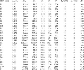
List of parameters for Poiseuille flow cases (P
 $i$
) and Couette flow cases (C
 $i$
).
 $U_{cl}$
is the mean centreline velocity and
 $U_{b}$
is the bulk velocity, both given in a frame attached to the lower wall.
 $\mathit{Re}_{B}=2hU_{b}/{\it\nu}$
is the bulk Reynolds number,
 $\mathit{Re}_{{\it\tau}}=hu_{{\it\tau}}/{\it\nu}$
is the friction Reynolds number,
 $\mathit{Re}_{T}=hU_{cl}/{{\it\nu}_{T}}_{cl}$
is the Reynolds number based on the turbulent viscosity and the mean velocity at the channel centreline.
 $N_{x}$
,
 $N_{y}$
,
 $N_{z}$
are the grid points in the streamwise, wall-normal, and spanwise directions.
 $L_{x}$
,
 $L_{z}$
are the box size in the wall-parallel directions, and
 $h$
is the channel half-height.

2. Numerical database
In this paper we exploit the DNS database of moderate/high-Reynolds-number Poiseuille and Couette flows developed in Bernardini et al. (Reference Bernardini, Pirozzoli and Orlandi2014) and Pirozzoli et al. (Reference Pirozzoli, Bernardini and Orlandi2014), together with an additional set of simulations at lower Reynolds numbers, as listed in table 1. The size of the computational domain in the wall-parallel plane was selected based on previous sensitivity studies, which have shown that it has to be larger in Couette flow simulations to accommodate large and persistent core eddies. In all reliable DNS, the two-point correlations are usually evaluated in the spanwise and streamwise directions to verify insensitivity to the size of the computational box. These are shown for Couette flow in Pirozzoli et al. (Reference Pirozzoli, Bernardini and Orlandi2014). The number of grid points was selected so as to keep the resolution nearly constant, in wall units, with
 ${\rm\Delta}x^{+}\lesssim 9$
and
 ${\rm\Delta}z^{+}\lesssim 6$
. A non-uniform grid was used in the
 $y$
direction, by clustering the points near the two walls. The numerical method is the same as described in Orlandi (Reference Orlandi2000), with the new feature that the equations are solved in a convective frame moving with the bulk velocity. This simple expedient leads to significant improvements of the numerical results, as documented in Bernardini et al. (Reference Bernardini, Pirozzoli, Quadrio and Orlandi2013). The simulations have been carried out in such a way that the mass flow rate (in a frame attached to the bottom wall) is kept constant in time, and it is the same for all the flow cases. Hence, the bulk velocity which appears in the definition of the bulk Reynolds number,
 $\mathit{Re}_{B}=2hU_{b}/{\it\nu}$
(where
 $h$
is the channel half-height), is also the same. In Couette flow, the bulk velocity is evaluated in a frame of reference attached to the lower wall, hence it also coincides with the centreline velocity. It must be pointed out that the simulations at low Reynolds number have been performed by taking fully developed turbulent cases as initial conditions. In particular, the P12 flow case has been used as the initial conditions for the P1–P11 Poiseuille simulations, and the C7 flow case has been used for the C1–C6 Couette simulations. These simulations can then be regarded as a nonlinear stability analysis to determine a critical Reynolds number.
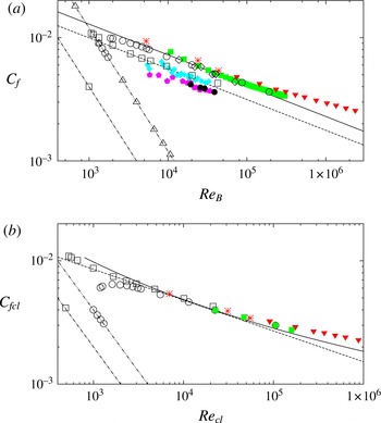
Friction coefficient versus Reynolds number for Poiseuille and Couette flows normalised with (a) bulk velocity and (b) centreline mean velocity. Open symbols indicate DNS data from the present work (circles for Poiseuille, and squares for Couette flow), from Orlandi (Reference Orlandi2011) (triangles), and from Hoyas & Jiménez (Reference Hoyas and Jiménez2006) (diamonds). Solid symbols correspond to experimental data for Poiseuille flow from Schultz & Flack (Reference Schultz and Flack2013) (squares), for Couette flow by El Telbany & Reynolds (Reference El Telbany and Reynolds1982) (circles), Robertson (Reference Robertson1959) (diamonds), Reichardt (Reference Reichardt1956) (pentagons), and for pipe flow by Wu & Moin (Reference Wu and Moin2008) (stars), McKeon et al. (Reference McKeon, Swanson, Zagarola, Donnelly and Smits2004) (downtriangles). The dashed-dot and dashed-dot-dot lines correspond to the theoretical friction laws for laminar Couette and Poiseuille flow, respectively. The dashed and solid lines represent power-law fits for turbulent flow: in (a)
 $C_{f}=0.0725\mathit{Re}_{B}^{-1/4}$
(solid line), and
 $C_{f}=0.0560\mathit{Re}_{B}^{-1/4}$
(dashed line); in (b)
 $C_{f}=0.048\mathit{Re}_{cl}^{-1/4}$
(dashed line). The solid line in (b) derives from solving the equation
 $(2/C_{fcl})^{1/2}=1/k\log (\mathit{Re}_{cl}(C_{fcl}/2)^{1/2})+B$
, with
 $k=0.4$
,
 $B=5$
.

3. Results
3.1. Friction factor
The friction coefficient
 $C_{f}=2u_{{\it\tau}}^{2}/U_{b}^{2}$
is shown in figure 1(a) as a function of
 $\mathit{Re}_{B}$
, for the flow cases listed in table 1, and for previous experimental and numerical studies, also including data for circular pipes at high
 $\mathit{Re}_{B}$
, to verify asymptotic trends. For reference, we also show the laminar laws for Poiseuille flow,
 $C_{f}=12/\mathit{Re}_{B}$
, and for Couette flow,
 $C_{f}=4/\mathit{Re}_{B}$
. For Couette flow at
 $\mathit{Re}_{B}=1000$
the flow is laminar, and a sharp transition from laminar to turbulent flow occurs at
 $\mathit{Re}_{B}\approx 1067$
, in rather good agreement with Orszag & Patera (Reference Orszag and Patera1980), but different from the transition threshold
 $\mathit{Re}_{B}=360$
found by Tillmark & Alfredsson (Reference Tillmark and Alfredsson1992), who looked for the formation of turbulent spots. The same behaviour is found for Poiseuille flow, with critical Reynolds number between
 $\mathit{Re}_{B}=1735$
and
 $\mathit{Re}_{B}=1867$
. Laboratory experiments on Couette flows are more complicated than for Poiseuille flow because of the need to minimise deformation of moving belts. These difficulties explain the relatively small number of papers reporting measurements on Couette flows (El Telbany & Reynolds Reference El Telbany and Reynolds1982; Aydin & Leutheusser Reference Aydin and Leutheusser1991). Figure 1(a) clearly shows the sharp transition for both flows. Although the linear velocity profile of laminar Couette flow is unconditionally stable to small disturbances, in the presence of large disturbances such as those given here, the critical Reynolds number is found to be lower than for Poiseuille flow. The reason is probably the formation of large eddies in the core of the channel, which are very weakly damped by the effect of viscosity. In addition, figure 1(a) shows that in the intermediate range of
 $\mathit{Re}_{B}$
the friction coefficient is rather well reproduced by power-law fits of the type
 $\mathit{Re}_{B}^{-1/4}$
, however with deviations both at low Reynolds number (with different behaviour of Couette and Poiseuille flow), and at high Reynolds number, as also discussed by Bernardini et al. (Reference Bernardini, Pirozzoli and Orlandi2014). It is also noteworthy that in this representation Couette flow yields about 23 % friction reduction as compared to Poiseuille flow, for given bulk velocity.
The wall shear stress can also be scaled with the centreline velocity, which is clearly constant for Couette flow, but varies with
 $\mathit{Re}_{B}$
for Poiseuille flow. By plotting
 $C_{fcl}=2u_{{\it\tau}}^{2}/U_{cl}^{2}$
as a function of
 $\mathit{Re}_{cl}=U_{cl}h/{\it\nu}$
, figure 1(b) shows significant collapse of the data of both flows on the curve
 $C_{fcl}=0.048\mathit{Re}_{cl}^{-1/4}$
for
 $\mathit{Re}_{cl}>2000$
, and different behaviour at low
 $\mathit{Re}_{cl}$
, which is due to the greater effect of the turbulent kinetic energy production in the central region at low
 $\mathit{Re}_{cl}$
, as discussed later on. It is interesting to note that the
 $C_{fcl}$
versus
 $\mathit{Re}_{cl}$
curves show good collapse across planar flows, and for pipe flow as well. As a reference, in figure 1(b) we also mark (with a thick grey line) the friction law obtained by assuming validity of the log law throughout the outer region, namely
 $U_{cl}^{+}-U^{+}=1/{\it\kappa}\log (y/h)$
. The better fit and the different trend obtained for the Couette data is suggestive of closer validity of the log law for this flow than for Poiseuille flow, even at low Reynolds number.
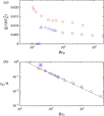
(a) Integrated turbulent kinetic energy over the whole channel, as a function of the bulk Reynolds number; (b) location of peak turbulent kinetic energy density as a function of the friction Reynolds number. Open circles are used for Poiseuille flow, and open squares for Couette flow. The dotted line in (b) indicates the fit
 $y_{q}/h=16/\mathit{Re}_{{\it\tau}}$
.

3.2. Turbulent kinetic energy
A further diagnostic of the flow state is the turbulent kinetic energy, integrated over the whole channel. Figure 2(a) gives
 $Q=\int \!q\text{d}y$
(where
 $q=\langle u_{i}^{2}\rangle /2$
), as a function of
 $\mathit{Re}_{B}$
for Poiseuille and Couette flows, and it provides a clear indication of the sharp transition from a laminar state with
 $Q=0$
, to a fully turbulent state with
 $Q\neq 0$
. The amount of turbulent kinetic energy for Couette flow is found to be greater than for Poiseuille flow for a given
 $\mathit{Re}_{B}$
, because of the contribution of turbulent production in the central region of the channel. In both flows the turbulent kinetic energy decreases with the Reynolds number after transition onset, implying that the near-wall layer where the energy is mainly concentrated becomes thinner as the Reynolds number is increased. A good indication for the concentration of kinetic energy is provided by the peak location of
 $q$
, hereafter denoted as
 $y_{q}$
. Figure 2(b) shows that
 $y_{q}$
decreases as
 $16/\mathit{Re}_{{\it\tau}}$
for both flows, hence it very nearly coincides with the point where the maximum of
 $\langle u^{\prime 2}\rangle$
occurs.
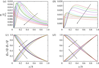
Turbulent kinetic energy profiles for (a) Poiseuille flow and (b) Couette flow. Cumulative kinetic energy from the lower wall
 $Q_{w}(y)$
and from the channel centreline
 $Q_{c}(y)$
, normalised by the total kinetic energy for (c) Poiseuille flow and (d) Couette flow. The arrows indicate the direction of increasing
 $\mathit{Re}_{{\it\tau}}$
.

The profiles of
 $q$
in outer units in figure 3(a,b) further show that the integral of
 $q$
for both flows is decreasing with
 $\mathit{Re}$
, and the size of the near-wall energy-containing structures (which can be estimated to be
 $2y_{q}$
), decreases with
 $\mathit{Re}$
. Having this size, these structures can move laterally and yield streamwise undulations, as is necessary for turbulence sustainment. If, on the other hand, the motion is constrained for any reason, a vortical state arises which does not correspond to developed turbulence. This confinement effect becomes evident at low Reynolds number, and the minimum value of
 $\mathit{Re}$
for sustaining turbulence corresponds to a case in which the size of the near-wall eddies becomes comparable to the channel half-width. The data obtained here agree well with the findings of Hamilton, Kim & Waleffe (Reference Hamilton, Kim and Waleffe1995) for Couette flow and of Jiménez & Moin (Reference Jiménez and Moin1991) for Poiseuille flow, in that the minimal lateral size of the computational box to sustain turbulent flow is approximately
 $100$
wall units. The lower value of the critical
 $\mathit{Re}_{{\it\tau}}$
found here is due to the wider computational domain, which allows turbulent structures greater freedom of lateral movement.
The aim of our simulations is to investigate whether the Reynolds number dependence of certain statistics observed in numerical and laboratory experiments on Poiseuille flow decreases or even completely disappears in Couette flow. Figure 3 shows that it is difficult to establish asymptotic trends based on plots of turbulent kinetic energy in outer units. In addition, since turbulent kinetic energy is unevenly distributed in the wall and in the outer regions, and differences are present between Poiseuille and Couette flow, we have evaluated the cumulated turbulence kinetic energies starting from the wall,
 $Q_{w}(y)=\int _{0}^{y}\!q\text{d}{\it\eta}$
, and starting from the channel centreline,
 $Q_{c}(y)=\int _{y}^{y_{c}}\!q\text{d}{\it\eta}$
. Since
 $Q$
varies with
 $\mathit{Re}_{B}$
, both
 $Q_{w}(y)$
and
 $Q_{c}(y)$
have been normalised with
 $Q$
. The crossing of the
 $Q_{w}(y)$
and the
 $Q_{c}(y)$
graphs then indicates the point where the contribution of the core turbulence equilibrates with the near-wall contribution. Figure 3(c) suggests that for Poiseuille flow the crossing distance varies at low Reynolds number, and that from
 $\mathit{Re}_{{\it\tau}}>150$
the amount of turbulence due to the near-wall structures is confined to the first 30 % of the channel. The linear scale in figure 3(a,b) highlights the different behaviour in the central region, which is decreasing for Poiseuille flow, and almost constant for Couette flow. The large contribution of the outer region for Couette flow leads to a linear behaviour of the cumulative kinetic energy in figure 3(d), which is found to be almost independent of the Reynolds number. In particular, it appears that Couette flow has an equal contribution from the turbulence coming from the near-wall region and from the core region. Given the Reynolds number independence observed in figure 3(d), it appears that Couette flow is a good candidate to study the effect of the outer region on the near-wall structures.
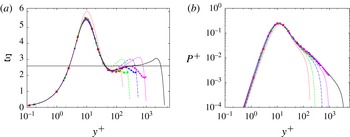
Profiles of (a) diagnostic function
 ${\it\Xi}=y^{+}\text{d}u^{+}/\text{d}y^{+}$
and (b) turbulent kinetic energy production, both given in wall units for Poiseuille flow (lines) and for Couette flow (symbols). Lines:
 $\mathit{Re}_{{\it\tau}}=180$
(dotted), 250 (dash-dotted), 500 (dash-dot-dot), 1000, (dashed) and
 $\mathit{Re}_{{\it\tau}}=4000$
(solid). Symbols:
 $Re_{{\it\tau}=180}$
(squares), 250 (circles), 500 (triangles) and 1000 (downward pointing triangles).

3.3. Diagnostic function and turbulent energy production
The profiles of the diagnostic function
 ${\it\Xi}$
are shown in figure 4(a) at the same
 $\mathit{Re}_{{\it\tau}}$
values for both flows, and at
 $\mathit{Re}_{{\it\tau}}=4000$
for Poiseuille flow only. As may be noticed, the present results at
 $\mathit{Re}_{{\it\tau}}=4000$
do not show any flat region as seen in figure 1b in Lozano-Duran & Jiménez (Reference Lozano-Duran and Jiménez2014), which is probably due to the use of a small computational box (
 $2{\rm\pi}\times {\rm\pi}h$
in the wall-parallel plane). From figure 4(a) it appears that a long region fitting the log law is not observed in the two flows considered here, at least at these moderate Reynolds numbers. However, the tendency of the Couette data at
 $\mathit{Re}_{{\it\tau}}=500,1000$
to superpose onto the Poiseuille data at
 $\mathit{Re}_{{\it\tau}}=4000$
(up to at least
 $y^{+}=300$
) indicates that Poiseuille flow has a greater Reynolds number dependence. Further increase of
 $\mathit{Re}$
for Poiseuille flow should lead to the same dependence on
 $\mathit{Re}$
as in Couette flow, which with good probability will consist of enlarging the width of the region tangent to the dotted line,
 ${\it\Xi}=1/0.386$
.
The turbulent kinetic energy production (
 $P=-\langle u^{\prime }v^{\prime }\rangle S$
, where
 $S=\text{d}\langle U\rangle /\text{d}y$
is the mean shear rate) is reported in figure 4(b). As expected, production is mainly concentrated in the near-wall region, and it increases as
 $y^{3}$
, reaching a maximum at the location where the turbulent shear stress,
 $-\langle u^{\prime }v^{\prime }\rangle$
equals the viscous stress,
 ${\it\nu}S$
. The maximum production in wall units (
 $P^{+}=P{\it\nu}/u_{{\it\tau}}^{3}$
) varies with
 $\mathit{Re}_{{\it\tau}}$
, approaching the value
 $0.25$
at high
 $\mathit{Re}_{{\it\tau}}$
. Poiseuille flow is characterised by zero production at the centre of the channel. On the other hand, Couette flow has non-zero turbulent production at the channel centreline. Near collapse of the production curves in wall units in Couette flow demonstrates that the main effect of the increase of
 $\mathit{Re}$
is the reduction of the centreline production. On the other hand, a large dependence on
 $\mathit{Re}$
appears for Poiseuille flow in the outer region, since production must vanish at the centreline. The interesting result is that production for Poiseuille flow at
 $\mathit{Re}_{{\it\tau}}=4000$
superposes onto production for Couette flow at
 $\mathit{Re}_{{\it\tau}}=1000$
. This is a further proof that Couette flow should be preferentially considered to study the effects of the outer region on the near-wall structures.
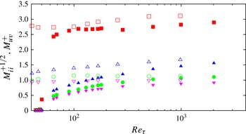
Maxima of turbulent stresses as a function of
 $\mathit{Re}_{{\it\tau}}$
: squares,
 $M_{uu}^{+}$
; circles,
 $M_{vv}$
; up-triangles,
 $M_{ww}^{+}$
; down-triangles,
 $M_{uv}^{+}$
. Open symbols are used for Couette flow, and solid symbols for Poiseuille flow.

3.4. Reynolds stress peaks
To emphasise differences between Poiseuille and Couette flow it is worth looking at the variation of the peaks of the turbulent stresses with the Reynolds number. Hoyas & Jiménez (Reference Hoyas and Jiménez2006) found logarithmic growth of the streamwise and spanwise Reynolds stress peaks (expressed in wall units) with
 $\mathit{Re}_{{\it\tau}}$
, which is caused by the interaction between the outer and the inner turbulence structures, and claimed that simulations at higher
 $\mathit{Re}$
are necessary to have more energy in the large-scale outer-layer structures. In Couette flow the outer structures are generated by the mean velocity gradient at the centre of the channel even at low Reynolds number, hence it represents in a certain sense an extreme case of the Poiseuille flow. In figure 5 the maxima of the stresses of Poiseuille flow are compared with those of Couette flow as a function of
 $\mathit{Re}_{{\it\tau}}$
. In this respect, we recall that in Couette flow mean momentum balance implies constancy of the total stress,
 $$\begin{eqnarray}-\!\langle u^{\prime }v^{\prime }\rangle +{\it\nu}S={\it\tau}_{w}.\end{eqnarray}$$
Hence, maximum turbulent shear stress (say,
 $M_{uv}$
) occurs at the channel centreline, where (3.1) reduces to
 $$\begin{eqnarray}-\!\langle u^{\prime }v^{\prime }\rangle _{cl}^{+}+S_{cl}^{+}=1,\end{eqnarray}$$
where
 $S_{cl}^{+}=S_{cl}{\it\delta}_{v}/u_{{\it\tau}}$
is the mean shear at the centreline. Since
 $S_{cl}h/u_{{\it\tau}}$
is approximately constant with
 $\mathit{Re}_{{\it\tau}}$
(Pirozzoli et al.
Reference Pirozzoli, Bernardini and Orlandi2014), it follows that
 $S_{cl}^{+}\sim 1/\mathit{Re}_{{\it\tau}}$
, and
 $$\begin{eqnarray}1-M_{uv}^{+}\sim \frac{1}{\mathit{Re}_{{\it\tau}}}.\end{eqnarray}$$
From (3.2) it also follows that the the centreline turbulence production scales as
 $$\begin{eqnarray}P_{cl}^{+}=-\langle u^{\prime }v^{\prime }\rangle _{cl}^{+}S_{cl}^{+}\approx \frac{1}{\mathit{Re}_{{\it\tau}}},\end{eqnarray}$$
which is well satisfied by the DNS data shown in figure 4(b).
In Poiseuille flow, mean momentum balance implies linear variation of the total stress,
 $$\begin{eqnarray}-\!\langle u^{\prime }v^{\prime }\rangle +{\it\nu}S={\it\tau}_{w}(1-y/h).\end{eqnarray}$$
Assuming that the maximum turbulent shear stress occurs in the logarithmic layer (where
 $S\approx 1/(ky)$
, and
 $k$
is the Kármán constant), from (3.5) it follows that
 $$\begin{eqnarray}1-M_{uv}^{+}\sim \frac{2}{(k\mathit{Re}_{{\it\tau}})^{1/2}}.\end{eqnarray}$$
The two relations (3.3) and (3.6) are well satisfied by the present data, which yield (the figure is not shown)
 $1-M_{uv}^{+}=2.7/\mathit{Re}_{{\it\tau}}$
for Couette flow, and
 $1-M_{uv}^{+}=3.5/\sqrt{\mathit{Re }_{{\it\tau}}}$
for Poiseuille flow, thus suggesting low-Reynolds-number effects are more rapidly saturated in Couette flow.
The wall-normal stress
 $\langle v^{\prime 2}\rangle$
plays an important role in wall-bounded flows, as highlighted by Orlandi (Reference Orlandi2013), through a comparison between the profiles in wall units obtained from simulations of flows in the presence of smooth and rough walls. Figure 5 shows that for the flows here considered the variations of
 $M_{vv}^{+}$
with
 $\mathit{Re}_{{\it\tau}}$
are smaller than those of
 $M_{uu}^{+}$
and
 $M_{ww}^{+}$
, consistent with Townsend’s attached eddy hypothesis, discussed later on. This is particularly evident for the case of Couette flow. However, an upper theoretical limit for
 $\langle v^{\prime 2}\rangle ^{+}$
is not available, hence the high-Reynolds-number behaviour cannot be extrapolated. Figure 5 highlights that
 $\langle u^{\prime 2}\rangle ^{+}$
reaches a nearly flat behaviour at lower values of
 $\mathit{Re}_{{\it\tau}}$
in Couette flow than in Poiseuille flow. The lateral stress
 $\langle w^{\prime 2}\rangle ^{+}$
for Couette flow is still increasing at the values of
 $\mathit{Re}_{{\it\tau}}$
considered here, which may be related to the undulations of the large-scale eddies created in the central part of the channel.
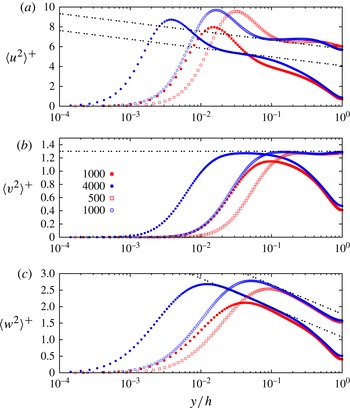
Profiles of normal Reynolds stresses for Poiseuille flow (solid symbols) and for Couette flow (open symbols): (a) streamwise, (b) wall-normal and (c) spanwise. The values of
 $\mathit{Re}_{{\it\tau}}$
are given in the legend. The dotted lines correspond to the theoretical logarithmic laws derived from Townsend’s attached eddy model, with values of the constants given in the text.

3.5. Townsend’s attached eddies
The validity of the theoretical predictions of Townsend (Reference Townsend1976) based on the attached eddy hypothesis have not yet received a wholly satisfactory confirmation from DNS (Jiménez Reference Jiménez2013) and experiments (Smits & Marusic Reference Smits and Marusic2013). Using a superposition of eddies with size proportional to the distance from the wall, Townsend (Reference Townsend1976, p. 154) proposed the following expression for the normal Reynolds stresses:
 $$\begin{eqnarray}\langle u^{2}\rangle ^{+}=C_{1}-D_{1}\log y/h,\quad \langle v^{2}\rangle ^{+}=C_{2},\quad \langle w^{2}\rangle ^{+}=C_{3}-D_{3}\log y/h,\end{eqnarray}$$
with the constants depending on the geometry of the attached eddies. The validity of these laws was tested through pipe experiments (Hultmark et al.
Reference Hultmark, Vallikivi, Bailey and Smits2012), by fitting measurements of
 $\langle u^{2}\rangle ^{+}$
in the logarithmic region
 $(10^{3}<y^{+}<10^{4})$
(in outer units,
 $0.1<y/h$
). Jiménez (Reference Jiménez2013) also attempted to fit DNS data for
 $0.1<y/h$
. From our data, and in particular from the spanwise turbulence intensity
 $\langle w^{2}\rangle ^{+}$
, figure 6(c) shows that indeed a good fit with the logarithmic law is found up to a distance
 $y/h\approx 0.1$
, within a layer widening at higher Reynolds numbers, with
 $C_{3}=1.08$
,
 $D_{3}=0.386$
. The constant
 $C_{3}$
depends on the flow and then on the shape of the attached eddies, which at that distance are affected by the large-scale eddies in the central region. As such eddies are more energetic in the Couette flow, a larger additive constant is found than for Poiseuille flow (
 $C_{3}=1.78$
). Notably, the slope is found to be the same for the two flows,
 $D_{3}=0.386$
.
It must be remarked that the distributions of the streamwise stress
 $\langle u^{2}\rangle$
are affected by production of turbulent kinetic energy, and in this sense the eddies related to this stress can be classified as active (although this term is commonly used to denote eddies carrying the shear stress), whereas the spanwise and the wall-normal stresses are only affected by redistribution terms, hence they can be regarded as inactive. In Poiseuille flow, turbulence kinetic energy production is to a large extent concentrated in the buffer layer, which is seen to affect the amplitude of
 $\langle u^{2}\rangle$
up to the log layer. In Couette flow the production in the outer region affects
 $\langle u^{2}\rangle$
to a greater extent, and no logarithmic range is observed. Comparison between figures 6(a) and 6(c) highlights the difference between the active and the inactive eddies (in our terminology), the former having a thinner region fitting Townsend’s law. Although Townsend’s hypothesis cannot be satisfactorily applied to the active eddies, application of the fit (figure 6) still yields
 $D_{1}=0.386$
, with
 $C_{1}=4.8$
for Poiseuille flow, and
 $C_{1}=5.78$
for Couette flow. It should be noted that the values of the constants for Poiseuille flow reported here are slightly different from those given by Bernardini et al. (Reference Bernardini, Pirozzoli and Orlandi2014), being evaluated here by fitting data given in outer units, in agreement with (3.7). Figure 6(b) clearly shows that Townsend’s hypothesis applies well to
 $\langle v^{2}\rangle ^{+}$
, and both flows have
 $C_{2}=1.3$
at high Reynolds numbers. From these results it appears that the attached eddies mainly carry
 $v$
and
 $w$
, and hence are mainly associated with streamwise vorticity, which is consistent with the conical eddies depicted in Townsend’s book (Townsend Reference Townsend1976, p. 157).
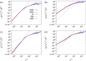
Turbulent stresses scaled with the local mean shear: (a) shear stress (
 ${\it\nu}_{T}/{\it\nu}$
), (b) streamwise stress, (c) normal stress, and (d) lateral stress, for Poiseuille flow (solid symbols) and Couette flow (open symbols). The values of
 $\mathit{Re}_{{\it\tau}}$
are given in the legend. The dashed lines denote the expected asymptotic behaviour in the near-wall layer and in the log layer (see text).

3.6. Scaling of turbulent stresses
As previously mentioned, the turbulent stresses scale rather well with the wall friction near the wall, but not in the outer region. Boussinesq (Reference Boussinesq1877) suggested a simple closure for turbulent flows, based on the introduction of an eddy viscosity
 ${\it\nu}_{T}$
to close the turbulent shear stress,
 $-\langle u^{\prime }v^{\prime }\rangle ={\it\nu}_{T}S$
. The ratio between the turbulent and the kinematic viscosity is then a quantity characterising wall-bounded flows. In the logarithmic region
 ${\it\nu}_{T}/{\it\nu}={\it\kappa}y^{+}$
, hence Poiseuille and Couette flows are expected to have the same trend. However, in Couette flow
 $\langle u^{\prime }v^{\prime }\rangle ^{+}$
is approximately constant, whereas it decreases linearly with the wall distance for Poiseuille flow, hence
 ${\it\nu}_{T}/{\it\nu}$
should deviate earlier from the linear trend in the latter case. Near the wall, continuity and the linear trend of
 $u^{\prime }$
lead to
 ${\it\nu}_{T}/{\it\nu}\approx y^{+3}$
, in both cases. Figure 7(a) indeed shows some degree of universality for the present wall-bounded flows at intermediate and high values of
 $\mathit{Re}$
. In this figure
 ${\it\nu}_{T}/{\it\nu}$
is also given for the lowest values of
 $\mathit{Re}_{{\it\tau}}$
for which the flow is turbulent, namely
 $\mathit{Re}_{{\it\tau}}=39$
for Couette. The good fit obtained for Couette flow once more suggests that the production of kinetic energy in the channel core promotes independence of the turbulent statistics from the Reynolds number. From all the data, at both high and low
 $\mathit{Re}$
, it is found that the turbulent Reynolds number evaluated at the centre of the channel,
 $\mathit{Re}_{T}=U_{cl}h/{{\it\nu}_{T}}_{cl}$
, as reported in table 1, has low values, implying that the velocity profiles in the core region should not largely differ from those in a laminar flow, as confirmed later on.
The data from the present set of DNS allow to investigate whether the local scaling also holds for the other (normal) turbulent stresses. A local scaling of the turbulent stresses was attempted by El Telbany & Reynolds (Reference El Telbany and Reynolds1982), based on data from laboratory measurements. They suggest the following expression for the near-wall region:
 $$\begin{eqnarray}\langle u^{2}\rangle ^{1/2}/u_{{\it\tau}}=A_{1}\,y^{+},\quad \langle v^{2}\rangle ^{1/2}/u_{{\it\tau}}=A_{2}\,y^{2+},\quad \langle w^{2}\rangle ^{1/2}/u_{{\it\tau}}=A_{3}\,y^{+},\end{eqnarray}$$
with the following set of coefficients:
 $A_{1}=0.28,A_{2}=0.005,A_{3}=0.08$
. For the same values of
 $\mathit{Re}_{{\it\tau}}$
as given in figure 7(a), figure 7(b–d) highlights the independence from
 $\mathit{Re}_{{\it\tau}}$
for Couette flows, and the previously discussed Reynolds number dependence of Poiseuille flows at low
 $\mathit{Re}$
. In the very near-wall region (
 $y^{+}<10$
) the profiles exhibit the same trends as observed by El Telbany & Reynolds (Reference El Telbany and Reynolds1982), however with the following set of constants:
 $A_{1}=0.447,A_{2}=0.01,A_{3}=0.283$
. The present data show that in the logarithmic region all the stresses normalised with the local shear grow linearly with
 $y^{+}$
, say
 $\langle u_{i}^{2}\rangle /S=B_{i}y^{+}$
, with different values for the constants,
 $B_{1}=2.5,B_{2}=0.386,B_{3}=1$
. For Couette flow the stresses reach a plateau toward the core region, whereas sharp growth occurs for Poiseuille flow, since
 $S=0$
at the centreline. The interesting result, which can be useful to extend existing turbulence models to the near-wall region, is the observed near collapse of
 ${\it\nu}_{T}/{\it\nu}$
onto a nearly universal curve, whereas the different behaviour in the core part of the channel is taken into account by the fact that mean shear directly enters all classical turbulence models, such as for instance the widely used Spalart–Allmaras model (Spalart & Allmaras Reference Spalart and Allmaras1994).
3.7. Turbulent kinetic energy budget
In this section we study the Reynolds number dependence of the turbulence kinetic energy terms, with the main goal of quantitatively establishing the effect of outer-layer structures on the near-wall region. For that purpose, in figure 8 we show the production, dissipation and transport terms in pre-multiplied form, is such a way that equal areas correspond to equal contributions, when data are reported in a semi-log scale. The pre-multiplied production for Poiseuille flow (figure 8
a) increases with the Reynolds number in the outer region, and it sharply drops off towards the centreline. In the same figure we also plot the pre-multiplied dissipation rate
 $y^{+}D^{+}$
, where
 $D={\it\nu}\langle u_{i}^{\prime }u_{i,jj}^{\prime }\rangle$
is the sum of viscous dissipation and diffusion, having finite value at the channel centre. In the equilibrium layer, production and dissipation approximately balance each other, corroborating the idea that in physical space a large part of the produced turbulent energy is locally dissipated. However, in order to understand how energy is redistributed within the channel, it is important to analyse the difference between the local production and dissipation, which is shown in figure 8(c,d). To check that the terms of the turbulent kinetic energy budget are correct it has been verified that balance is satisfied, i.e.
 $P+D=-T=(\text{d}/\text{d}y)(\langle v^{\prime }q^{\prime }\rangle +\langle v^{\prime }p^{\prime }\rangle )$
. From the plots of
 $y^{+}T^{+}$
for Poiseuille flow (figure 8
c) it is clear that in the buffer layer the production is larger than the local rate of dissipation, and this excess is transferred to the adjacent layers. This scenario is very weakly changed by Reynolds number variation. The effect of the Reynolds number appears to be mainly confined to the viscous sublayer region and to the logarithmic region, where the excess (respectively, defect) of
 $T$
is increasing with
 $\mathit{Re}_{{\it\tau}}$
. This observation can be either explained as a Reynolds number effect on the dynamics of the small scales, hence a violation of pure wall scaling, or as the result of non-local interactions (in physical space) between log-layer eddies and near-wall eddies. For Couette flow (figure 8
b,d) the Reynolds number independence in the wall region is emphasised by the bulk production and dissipation rate. Even though production does not vanish at the channel centreline, the rate of dissipation increases. Comparison between figures 8(c) and 8(d) leads to the conclusion that a strong similarity in turbulent transport exists in Poiseuille and Couette flows, although the Reynolds number effect on the viscous sublayer seems to be more modest in the latter case. In Couette flow non-zero production is maintained in the core region, which however remains a region with prevalent dissipation, as in Poiseuille flow.
Profiles of pre-multiplied (a,b) production and viscous dissipation
 $+$
diffusion, and (c,d) turbulent transport. (a,c) Poiseuille flow at
 $\mathit{Re}_{{\it\tau}}=180,550,1000$
, 4000, and (b,d) Couette flow at
 $\mathit{Re}_{{\it\tau}}=180,250,500,1000$
.

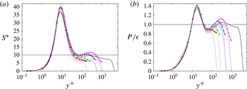
Profiles of (a) shear-rate parameter
 $S^{\ast }$
and (b) production-to-dissipation ratio for Poiseuille flow (lines) and Couette flow (symbols). Lines:
 $\mathit{Re}_{{\it\tau}=180}$
(dotted), 500 (dash-dot-dotted), 1000 (dashed) and 4000 (solid). Symbols:
 $\mathit{Re}_{{\it\tau}=180}$
(squares), 250 (circles), 500 (triangles) and 1000 (downward pointing triangles).

To understand whether the strength of the outer structures is comparable to that of the energetic buffer-layer structures, it is useful to consider the shear parameter
 $S^{\ast }=Sq/{\it\epsilon}$
, i.e. the ratio between the turbulent and the mean flow time scales (Lee, Kim & Moin Reference Lee, Kim and Moin1990). The profiles given in figure 9(a) show a reduced dependence of
 $S^{\ast }$
on the Reynolds number up to
 $y^{+}\approx 30$
, especially for Couette flow. In the outer region, at
 $\mathit{Re}_{{\it\tau}}=180$
, in agreement with the conclusions of Lee et al. (Reference Lee, Kim and Moin1990),
 $S^{\ast }$
is close to
 $5$
, which implies that elongated coherent structures cannot form. On the other hand, in Couette at
 $\mathit{Re}_{{\it\tau}}=250$
(Pirozzoli, Bernardini & Orlandi Reference Pirozzoli, Bernardini and Orlandi2011), we find
 $S^{\ast }\approx 10$
, which can be regarded as a lower threshold for observing coherent streamwise structures (Lee et al.
Reference Lee, Kim and Moin1990). A similar value of
 $S^{\ast }$
is achieved in Poiseuille only at
 $\mathit{Re}_{{\it\tau}}=4000$
. The figure further corroborates the observation that in Couette flow the large outer eddies have a limited Reynolds number dependence, and in fact the distributions of the shear parameter for the flow cases
 $\mathit{Re}_{{\it\tau}}=500$
and
 $\mathit{Re}_{{\it\tau}}=1000$
are superposed on each other, to a large extent.
In figure 9(b) we show the production-to-dissipation ratio,
 $P/{\it\epsilon}$
. The figure indicates that in Couette flow this ratio stays larger than unity over a large fraction of the channel, namely
 $0.2<y/h<0.6$
at
 $\mathit{Re}_{{\it\tau}}=500$
, and
 $0.1<y/h<0.5$
at
 $\mathit{Re}_{{\it\tau}}=1000$
, which corresponds to the layer where energetic outer streamwise structures are located (Pirozzoli et al.
Reference Pirozzoli, Bernardini and Orlandi2014). A similar production excess is also observed in Poiseuille flow, although it is limited to a narrower layer, and it is initiated at higher Reynolds number. For both flows, the dissipation rate overcomes production around the channel centreline.
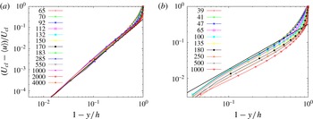
Profiles of velocity defect (
 $(U_{cl}-\langle u\rangle )/U_{cl}$
versus
 $1-y/h$
) for (a) Poiseuille flow (the dashed straight line is proportional to
 $(1-y/h)^{2}$
, (b) for Couette (the dashed straight line is proportional to
 $(1-y/h)$
). The values of
 $\mathit{Re}_{{\it\tau}}$
are indicated in the legend.

3.8. Core velocity profiles
It has been previously mentioned that the turbulent Reynolds number
 $\mathit{Re}_{T}$
does not vary much with the bulk Reynolds number, and it has rather small values (see table 1). Therefore it seems reasonable to assume that the flow in the channel core behaves much like an equivalent laminar flow, and one should expect parabolic profiles for Poiseuille flow, and linear profiles for Couette flow. Pirozzoli (Reference Pirozzoli2014) and Bernardini et al. (Reference Bernardini, Pirozzoli and Orlandi2014) indeed showed that in Poiseuille flow the mean velocity profiles are well fitted by parabolas around the channel centreline. In order to verify this behaviour, in figure 10 we show the scaled velocity defect
 $(U_{cl}-\langle u\rangle )/U_{cl}$
as a function of the distance from the centreline, in a log–log diagram. Figure 10(a) shows that the parabolic profiles are preserved in a wide portion of the channel in Poiseuille flow, which becomes wider for higher Reynolds number. Similar conclusions also apply to Couette flow (figure 10
b), in which the mean velocity profiles at the channel centreline tend to follow a linear behaviour. Hence, we may conclude that drastic changes are not expected even at higher Reynolds number in the core part of channel flows.
4. Conclusions
A comparison of the flow properties of turbulent Poiseuille and Couette flows has been carried out in a wide range of Reynolds numbers, from the transitional well into the fully turbulent regime. Some interesting observations can be made, which can be of some theoretical but also practical use. From a global standpoint, we have investigated the behaviour of the friction coefficient and of the total kinetic energy (the latter never considered in previous studies). It has been observed that in both Poiseuille and Couette flows the friction coefficient and the overall kinetic energy decrease with increasing Reynolds number. In particular, the friction coefficient is approximately the same for the two flows, when data are made non-dimensional with respect to the centreline properties, hence supporting the universality of the wall law. However, if the friction curve is reported as a function of the bulk properties it is found that, for given mass flow rate, Couette flow yields less resistance than Poiseuille flow, probably up to very high Reynolds number. A similar behaviour is also observed for the integrated kinetic energy, which abruptly changes from zero to a maximum corresponding to the transition threshold. These observations suggest the possible use of devices based on moving belts for fluid transport in order to minimise frictional losses, and the effectiveness of Couette flows at low Reynolds number in promoting turbulent diffusion.
To highlight differences between the two flows in the outer layer, the turbulent kinetic energy profiles have been analysed. A clear idea is obtained by the profiles of the integrals of
 $q$
evaluated starting from the wall (
 $Q_{w}(y)$
) and starting from the centre (
 $Q_{c}(y)$
). For Poiseuille flow balance occurs at
 $y/h=0.3$
and for Couette flow at
 $y/h=0.5$
, leading to the conclusion that the near-wall region where most energy production is located has a greater importance in Poiseuille than in Couette flow. It has also been observed that the profiles are linear for Couette flow at high Reynolds number.
The comparison of the Reynolds stress components has shown greater Reynolds number dependence in Poiseuille flow. This was also found by Hoyas & Jiménez (Reference Hoyas and Jiménez2006), and motivated the idea of studying high-Reynolds-number effects in experiments and in numerical simulations. Couette flow leads to quite a different behaviour, with unexpected results previously not observed due to the lack of experiments and DNS in a wide range of Reynolds numbers. It has been observed here that the normal (
 $\langle v^{\prime 2}\rangle$
) and the turbulent stress (
 $\langle u^{\prime }v^{\prime }\rangle$
) profiles very nearly collapse with
 $\mathit{Re}_{{\it\tau}}$
, whereas the maximum shear stress approaches unity as
 $1/\mathit{Re}_{{\it\tau}}$
, and the centreline turbulence kinetic energy production also decays as
 $1/\mathit{Re}_{{\it\tau}}$
. Stronger Reynolds number dependence was observed for
 $\langle w^{\prime 2}\rangle$
, which is mainly associated with the spanwise undulations of the large outer-layer structures generated by the production term, which directly only acts on
 $\langle u^{\prime 2}\rangle$
. These observations can be interpreted by regarding the Couette flow as a sort of limit, to which Poiseuille flow tends as the Reynolds number increases.
The different values of the peaks and the shape of the profiles for all the stresses in wall turbulent flows is one of the reasons why it is rather difficult to have satisfactory low-Reynolds-number turbulence models for the wall region. The Reynolds number dependence is large if the stresses are scaled in outer units, and it reduces when the stresses are scaled in wall units, with reduced dependence on the distance of the maxima, in particular for
 $\langle u^{\prime 2}\rangle$
. By scaling the stresses with a local shear velocity (El Telbany & Reynolds Reference El Telbany and Reynolds1982), a satisfactory collapse of the profiles in the near-wall region and in the logarithmic region is obtained for both Poiseuille and Couette flow. Hence, we expect that simple algebraic models can be applied to the near-wall region and to the logarithmic layer yielding satisfactory prediction of wall turbulent flows, which also applies to the normal stresses. The present DNS have further shown that near the channel centreline turbulent Poiseuille flows have laminar-like parabolic velocity profiles, whereas laminar-like linear profiles are recovered for Couette flows. Indeed, in both flows it has been observed that the effective Reynolds number based on the centreline velocity and turbulent viscosity
 $\mathit{Re}_{T}=U_{cl}h/{\it\nu}_{T}$
, is rather low, being approximately 50 for Couette flows, and slowly increasing with
 $\mathit{Re}_{{\it\tau}}$
from 200 to 400 for Poiseuille flows.
The mechanisms of energy transfer within the channel have been analysed by monitoring the ratio of turbulent kinetic energy production and dissipation rate, and the turbulent transport term. These quantities offer a more precise idea of Reynolds number effects on outer/inner-layer interactions than the production term alone, which is more easily evaluated in experiments. Our data show a noticeable lack of universality in the transfer term, which is mainly concentrated in the viscous sublayer and in the logarithmic layer. These differences imply excess of production over dissipation in the logarithmic layer caused by the onset of energetic large eddies as was observed in this paper. Regarding the differences in the near-wall region, these can be equally well explained by accepting violations of pure wall scaling, hence increased activity of the near-wall eddies at high Reynolds number, or long-range influence of eddies in the log-layer on the near-wall region through imprinting/modulations effects discussed in previous publications (Mathis, Hutchins & Marusic Reference Mathis, Hutchins and Marusic2009; Pirozzoli et al. Reference Pirozzoli, Bernardini and Orlandi2011). In fact, the extra energy feeding from the core eddies seems to be rather small, even in the extreme case of Couette flow, and it mainly acts in the sense of reducing the Reynolds number dependence observed in Poiseuille flow.
Acknowledgement
We acknowledge that some of the results reported in this paper have been achieved using the PRACE Research Infrastructure resource FERMI based at CINECA, Casalecchio di Reno, Italy.