
1. Introduction
Wake-ingesting propellers in marine and aeronautical applications such as ships (Guo & Zou Reference Guo and Zou2022; Qin et al. Reference Qin, Huang, Pan, Chao, Luo and Han2022) and aircraft (Hall Reference Hall2017; Lv et al. Reference Lv, Ragni, Hartuc, Veldhuis and Rao2017) are commonly found, and the fuel efficiency and integration flexibility of the pusher-propeller configuration make it an attractive candidate with increased interest for future low-speed aircraft designs (Arnhem, Vos & Veldhuis Reference Arnhem, Vos and Veldhuis2019; Tiseira Izaguirre et al. Reference Tiseira Izaguirre, García-Cuevas González, Quintero Igeño and Varela Martínez2022). Propellers ingesting non-uniform and turbulent flows can be the dominant source of unsteady aerodynamic forces and noise that creates serious concerns, including the operational restrictions of aircraft (Pardo & Hall Reference Pardo and Hall2021) and the detriment of concealment attributes for submarines (Blake Reference Blake2017), where the urgent need for noise control strategies has emerged. The need for noise control requires a deepened understanding of noise generation mechanisms and more accurate source identification methods, which motivate the current study.
A common phenomenon of wake-ingestion is the tonal noise generated by the interaction between the rotor blades and the coherent structures in the wake. The tones at harmonics of the blade passing frequency (BPF) are observed clearly in the experiments of aerofoil–rotor configurations. Catlett, Anderson & Stewart (Reference Catlett, Anderson and Stewart2012) have measured the thrust and noise of a seven-bladed propeller ingesting wakes from an upstream aerofoil model, which both show spectral peaks at the BPF and its harmonics. Catlett et al. (Reference Catlett, Anderson and Stewart2012) have also proposed an improved noise prediction model to account for the inhomogeneity and anisotropy of the wake that can better capture the wake-ingestion features. Brown et al. (Reference Brown, Fleming, Langford, Walton, Ng, Schwartz, Wisda and Burdisso2021) have compared the noise of a two-bladed propeller ingesting pylon wakes with thin and thick trailing edges. While both set-ups produce louder tonal noise than the isolated propeller, the pylon with a thick trailing edge could result in an even louder noise. The tonal noise is also found in other aeroacoustic applications where the wake–rotor interaction exists, e.g. counter-rotating open rotors (Horváth Reference Horváth2015; Kingan & Parry Reference Kingan and Parry2019) and the pumpjet propulsor (Qin et al. Reference Qin, Pan, Lee, Huang and Shi2019; Xiong et al. Reference Xiong, Rui, Lu, Zhang and Huang2022).
Ingestion of turbulent wakes has also been investigated recently, including ingestions of grid-generated homogeneous turbulence (Wojno, Mueller & Blake Reference Wojno, Mueller and Blake2002; Anderson, Catlett & Stewart Reference Anderson, Catlett and Stewart2015), inhomogeneous turbulence inside an engine duct (Robison & Peake Reference Robison and Peake2014), and turbulent cylinder wakes (Alexander et al. Reference Alexander, Molinaro, Hickling, Murray, Devenport and Glegg2016; Wang, Wang & Wang Reference Wang, Wang and Wang2021). The physical understanding of the turbulence-ingestion noise has been developed accordingly, and two special features of the turbulence-ingestion noise problem have been identified. The first feature, ‘haystacking’, which refers to the spectral humps at the BPF and its harmonics, is attributed to the stretched ingested turbulent structures (Majumdar & Peake Reference Majumdar and Peake1998) and the interaction between the ingested turbulence eddies and the successive blades (Murray et al. Reference Murray, Devenport, Alexander, Glegg and Wisda2018). The second feature, ‘blue shifting’, which refers to the shift of haystacking peaks to the right of the BPF and its harmonics (Martinez Reference Martinez1996), has been explained by various analytical models (Martinez Reference Martinez1996; Murray et al. Reference Murray, Devenport, Alexander, Glegg and Wisda2018; Huang Reference Huang2023).
Although progress has been made in turbulence-ingestion noise study, high-fidelity numerical studies along with aeroacoustic source analysis that help to illuminate the underlying fluid mechanics are still rare, and deepened insight and understanding of the noise sources and noise generation mechanism underneath are still needed. Such source analysis methods could also benefit studies of similar problems, e.g. the propeller–rudder interaction (Posa, Felli & Broglia Reference Posa, Felli and Broglia2022c) and the fan–outlet-guide-vane interaction (Casalino et al. Reference Casalino, Avallone, Gonzalez-Martino and Ragni2019).
Figure 1 demonstrates the most popular source localization and identification approaches, which are classified into two categories, acoustic imaging and acoustic analogy (Deneuve et al. Reference Deneuve, Druault, Marchiano and Sagaut2010), according to whether the far-field signals or the near-field flow field solutions are used to reconstruct noise sources. The acoustic imaging approach originates from the experimental measurements, and various methods have been proposed to reconstruct aeroacoustic sources based on partial information of the acoustic field, e.g. the time-reversal technique (Padois et al. Reference Padois, Prax, Valeau and Marx2012), acoustic holography (Maynard, Williams & Lee Reference Maynard, Williams and Lee1985) and beamforming (Huang et al. Reference Huang, Bai, Vinogradov and Peers2012). Among those methods, beamforming is an experimental technique that enables a sensor array to reconstruct equivalent acoustic sources and has been popular in aeroacoustic experiments for its robust performance with the existence of background noise and external interferences. Moreover, numerical beamforming has been proposed recently to reconstruct aeroacoustic sources from computational fluid dynamics results. Compared with the experimental counterpart, numerical beamforming eliminates the need for special facilities such as anechoic wind tunnels, and benefits from the absence of background noise from wind tunnels and invasive measuring equipment (Adam, Menoret & Ricot Reference Adam, Menoret and Ricot2009; Lockard et al. Reference Lockard, Humphreys, Khorrami, Fares, Casalino and Ravetta2017). Hence, as an emerging technique, numerical beamforming has been applied to various aeroacoustic applications in the past decade, e.g. side-view mirrors (Evans, Hartmann & Delfs Reference Evans, Hartmann and Delfs2019), airframes and aerofoils (Lockard et al. Reference Lockard, Humphreys, Khorrami, Fares, Casalino and Ravetta2017; Khorrami, Konig & Fares Reference Khorrami, Konig and Fares2021), and jet applications (Panickar, Sinha & Murray Reference Panickar, Sinha and Murray2013; Pignier, O'Reilly & Boij Reference Pignier, O'Reilly and Boij2016).
A sketch of the two approaches for localizing and identifying the aeroacoustic sources.

The noise generated by rotor blades has been investigated using beamforming methods both experimentally and numerically. For the large-size wind turbines, the noise sources are well captured by Nelson et al. (Reference Nelson, Cain, Raman, Chan, Saunders, Noble, Engeln, Dougherty, Brentner and Morris2012) and Ramachandran, Raman & Dougherty (Reference Ramachandran, Raman and Dougherty2014), whose results also suggest that the low-frequency sources are indistinguishable, such that the noise from the blade and the mechanical box can be separated only at high frequencies. For a model rotor of a smaller size, Alexander et al. (Reference Alexander, Molinaro, Hickling, Murray, Devenport and Glegg2016) and Hickling et al. (Reference Hickling, Alexander, Nicholas, Devenport and Glegg2017) have localized the broadband sources of ingestion noise of cylinder wakes, where the location of low-frequency sources on the propeller blades is not fully recognizable. Horváth (Reference Horváth2015) and Tokaji, Soós & Horváth (Reference Tokaji, Soós and Horváth2020) have measured the tonal and broadband noise sources of counter-rotating open rotors, and identified the typical locations of various types of aeroacoustic sources. Chen et al. (Reference Chen, Peng, Liem and Huang2020a) have performed particle image velocimetry (PIV) measurements to acquire the flow field, and conducted wavelet-based beamforming to capture the moving sources from a propeller ingesting aerofoil wakes, which show consistency of source generation with the interaction flow phenomenon. More recently, by using acoustic signals sampled from various artificial microphone arrays on different planes, Chen, Jiang & He (Reference Chen, Jiang and He2022) have provided a three-dimensional acoustic imaging technique for the study of propeller noise. However, the above works on smaller-size rotors hardly provide imaging results at frequencies lower than 1 kHz due to the resolution issue. Furthermore, their results have been used mostly to identify the most dominant sources, rather than to show the distribution of all sources. Hence the current work considers providing complementary results about aeroacoustic sources, especially at low to mid frequencies.
The second approach to identifying aeroacoustic sources is rooted in acoustic analogies. To derive the acoustic analogies, the flow-governing equations are reorganized from their original nonlinear form  $N(\boldsymbol {q})=0$ to the wave-propagation form
 $L\boldsymbol {q}=S(\boldsymbol {q})$ with source terms (Wang, Freund & Lele Reference Wang, Freund and Lele2006), where
 $\boldsymbol {q}$ is a flow solution that includes sound, and
 $N$ and
 $L$ denote the corresponding operators. The right-hand-side term
 $S(\boldsymbol {q})$ from the acoustic analogies is recognized as the aeroacoustic source. The pioneering work of Lighthill (Reference Lighthill1952) modelled the sound generation from the quadrupole-type sources by rearranging the Navier–Stokes equations. Lighthill's analogy has been extended further by Ffowcs Williams & Hawkings (Reference Ffowcs Williams and Hawkings1969) for arbitrary moving surfaces, which becomes probably the most-used acoustic analogy in aeroacoustic simulations. Moreover, it is also worthwhile to mention other well-known acoustic analogies that have been proposed for vortex-generated sources (Powell Reference Powell1964; Howe Reference Howe1975) and jet noise sources (Lilley Reference Lilley1996; Freund Reference Freund2001).
In the Ffowcs Williams and Hawkings (FW–H) equation, noise sources are grouped into monopole (thickness), dipole (loading) and quadrupole (turbulence) sources. At low Mach numbers, it is well known that the loading part is the dominant source (Wang et al. Reference Wang, Wang and Wang2021). Hence a straightforward idea is to examine surface pressure fluctuations to infer the distribution of loading noise. Therefore, the root-mean-square (r.m.s.) value of surface pressure fluctuations has often been used as the indicator of the strength of the loading noise sources, which has found applications for landing gear (Rougier et al. Reference Rougier, Bouvy, Casalino, Appelbaum and Kleinclaus2015), hydrofoil–propeller combinations (Posa, Broglia & Felli Reference Posa, Broglia and Felli2022a; Posa, Felli & Broglia Reference Posa, Felli and Broglia2022b) and rotating blades (Keller, Kumar & Mahesh Reference Keller, Kumar and Mahesh2018; Shur et al. Reference Shur, Strelets, Travin, Christophe, Kucukcoskun, Schram, Sack and Åbom2018; Zhou, Wang & Wang Reference Zhou, Wang and Wang2021). These works revealed the places with strong pressure fluctuations, while their direct relationship with the sound emission remains unclear. Alternatively, the time derivative of surface pressure has been adopted to represent the noise sources for various aeroacoustic applications (Maruta & Kotake Reference Maruta and Kotake1983; Tan et al. Reference Tan, Yang, Tan, Wu and Zhang2018; Casalino et al. Reference Casalino, Avallone, Gonzalez-Martino and Ragni2019) as well as rotor noise investigations (Wasala et al. Reference Wasala, Storey, Norris and Cater2015; Jiang et al. Reference Jiang, Wu, Chen, Zhou, Zhong, Zhang, Zhou and Chen2022; Zhou, Wang & Wang Reference Zhou, Wang and Wang2022). While for stationary surfaces it has been revealed that the main noise contribution to the far-field noise is due to the time derivative of surface pressure based on Curle's integral formula (Maruta & Kotake Reference Maruta and Kotake1983; Tan et al. Reference Tan, Yang, Tan, Wu and Zhang2018), a discussion on rotating surfaces is still missing. Therefore, what lacked in previous works is the theoretical explanation and derivation based on the FW–H equation, which will be addressed in this paper.
In the present work, a comprehensive aeroacoustic source analysis is performed to examine the noise generation mechanisms of a two-bladed propeller ingesting the wake from an upstream aerofoil. The large eddy simulation is first validated and then executed to obtain the near-field flow results. The FW–H equation is solved to calculate noise signals acquired at the microphone arrays to feed into the numerical acoustic imaging process using both classical and recently developed wavelet-based beamforming techniques. To improve the spatial resolution of source localizations, a near-field aeroacoustic source analysis approach is developed, and specific source terms are derived from the FW–H equation, which can be calculated directly from the simulated near-field flow results. The properties of aeroacoustic sources and their correlation to the flow features are investigated. Last, but not least, the two source-identifying approaches are compared and discussed.
The remaining part of this paper is organized as follows. Section 2 first introduces the theory of the numerical beamforming approach. Next, the near-field aeroacoustic analysis approach is developed, with a detailed derivation of source terms from the FW–H equation. The near-field aeroacoustic analysis enables a direct mapping from computational fluid dynamic solutions to near-field aeroacoustic sources without the intermediate steps of far-field noise signal calculation and beamforming reconstruction, which constitutes the main contribution of this work from the theoretical perspective. Section 3 presents the details and validation of the large eddy simulation. Section 4 provides the acoustic imaging results using numerical beamforming. Section 5 applies the near-field aeroacoustic analysis approach to study the aeroacoustic sources on the propeller surface and their physical mechanisms, as well as the far-field noise properties. Section 6 concludes the current work and findings.
2. Sources analysis methods
In this section, the theoretical background and derivations for the numerical beamforming and the proposed near-field aeroacoustic source analysis are given. The former technique is not new in experiments but became available to the numerical community only recently (Fleury & Chélius Reference Fleury and Chélius2013; Horváth, Envia & Podboy Reference Horváth, Envia and Podboy2014; Ma Reference Ma2017; Chen et al. Reference Chen, Jiang and He2022) owing to the great advances in computational capability. The latter technique is a new approach proposed in this work in reaction to certain inadequacies (such as low reconstruction resolution and complexity in the feedforward reconstruction model) of the former. For the latter, the derivations are based on the acoustic analogy along with certain assumptions and simplifications specifically for the problem of interest. Readers who are interested only in the physics of turbulence-ingesting noise problems may choose to skip to the next section and just refer to (2.5) for the beamforming analysis and (2.15) for near-field aeroacoustic analysis.
2.1. Beamforming in acoustic imaging
In this work, both the classical beamforming and the novel wavelet-based beamforming methods are used to produce aeroacoustic source maps of the propeller. The basic idea of the beamforming technique is introduced here briefly for those unfamiliar with this imaging method. For a more detailed introduction to beamforming for aeroacoustic applications, interested readers are referred to Huang et al. (Reference Huang, Bai, Vinogradov and Peers2012) for classical beamforming and Chen et al. (Reference Chen, Peng, Liem and Huang2020a) for wavelet-based beamforming.
In the classical frequency-domain beamforming, the acoustic pressure signal  $p(\,\boldsymbol {y},t)$ is first sampled from each sensor of the array, where
 $\boldsymbol {y}$ gives the associated spatial coordinates. Then the frequency-domain signal
 $P(\,\boldsymbol {y},f)$ is obtained by applying a Fourier transform. Next, the data from multiple sensors are collected to construct the so-called cross-spectral matrix (CSM):
 \begin{equation} \boldsymbol{\mathsf{A}} = \boldsymbol{Y}(\,\boldsymbol {y},f) \boldsymbol{\cdot} \boldsymbol{Y}^*(\,\boldsymbol {y},f), \end{equation}
where  $\boldsymbol {Y}(\,\boldsymbol {y},f)=[P(\,\boldsymbol {y}_1,f), \ldots, P(\,\boldsymbol {y}_n,f)]$ is the vector form of the array measurements,
 $\boldsymbol {y}_n$ gives the coordinates of the
 $n$th array sensor, and
 $({\cdot })^*$ denotes the complex conjugate. Diagonal removal of the CSM is applied to mitigate the interference and background noise. Finally, the imaging output is computed by
 \begin{equation} b(\boldsymbol{x},f) = \boldsymbol{w}^*(\boldsymbol{x}) \boldsymbol{\cdot} \boldsymbol{\mathsf{A}} \boldsymbol{\cdot} \boldsymbol{w}(\boldsymbol{x}), \end{equation}
where  $\boldsymbol {x}$ is the location of the imaging point,
 $\boldsymbol {w}(\boldsymbol {x}) = \boldsymbol {G}(\boldsymbol {x},\boldsymbol {y}) / \Vert \boldsymbol {G}(\boldsymbol {x},\boldsymbol {y}) \Vert$ is the beamforming weight vector,
 $\Vert {\cdot } \Vert$ denotes the L2-norm, and
 $\boldsymbol {G}(\boldsymbol {x},\boldsymbol {y}) = [G(\boldsymbol {x},\boldsymbol {y}_1), \ldots, G(\boldsymbol {x},\boldsymbol {y}_n)]$ is the free-space Green's function. Thus the source distribution and the associated source amplitude at any frequency are obtained by calculating iteratively
 $b(\boldsymbol {x},f)$ over a given plane.
For wavelet-based beamforming, the procedure is similar but slightly modified to include the temporal dimension. The time–frequency domain data  $P(\,\boldsymbol {y},t,s)$ are obtained from the sensor signals by the continuous wavelet transform
 \begin{equation} P(\,\boldsymbol {y},t,s) = \frac{1}{s} \int_{-\infty}^{\infty} \psi^*\left(\frac{\tau-t}{s}\right) p(\,\boldsymbol {y},\tau) \,{\rm d}\tau, \end{equation}
where  $\psi$ is the Morse wavelet, and
 $s$ is the scale parameter. The CSM is then constructed with a form similar to (2.1):
 \begin{equation} \boldsymbol{\mathsf{A}} = \boldsymbol{Y}(\,\boldsymbol {y},t_e,s) \boldsymbol{\cdot} \boldsymbol{Y}^*(\,\boldsymbol {y},t_e,s), \end{equation}
where  $\boldsymbol {Y}(\,\boldsymbol {y},t_e,s)=[P(\,\boldsymbol {y}_1,t_1,s), \ldots, P(\,\boldsymbol {y}_n,t_n,s)]$, and
 $t_n$ is the corresponding receiving time of the noise emitted at time
 $t_e$. Finally, the imaging output is computed by
 \begin{equation} b(\boldsymbol{x},s,t_e) = \boldsymbol{w}^*(\boldsymbol{x},t_e) \boldsymbol{\cdot}\boldsymbol{\mathsf{A}} \boldsymbol{\cdot} \boldsymbol{w}(\boldsymbol{x},t_e), \end{equation}
where  $\boldsymbol {w}(\boldsymbol {x},t_e) = \boldsymbol {G}(\boldsymbol {x},\boldsymbol {y},t_e) / \Vert \boldsymbol {G}(\boldsymbol {x},\boldsymbol {y},t_e) \Vert$, and
 $\boldsymbol {G}(\boldsymbol {x},\boldsymbol {y},t_e) = [G(\boldsymbol {x},\boldsymbol {y}_1,t_e), \ldots, G(\boldsymbol {x},\boldsymbol {y}_n, t_e)]$ is the free-space Green's function for moving sources (Chen et al. Reference Chen, Peng, Liem and Huang2020a). In this way, the source maps at different time
 $t_e$ are obtained in the time–frequency domain.
2.2. Near-field aeroacoustic source analysis
One of the main drawbacks of the numerical beamforming approach is that the resolution of the sources is frequency-dependent and can result in inadequate resolutions at lower frequencies. More of this limitation of the beamforming approach will be demonstrated and discussed in § 4. In this subsection, we propose a high-resolution near-field aeroacoustic source analysis approach that reconstructs directly the aeroacoustic sources on a rotating surface from the computational fluid dynamic solutions. The derivation starts from the classical FW–H equation, which, however, can provide only the far-field noise signals. By introducing the assumptions of low Mach number flow, constant rotating motion and far-field receivers, the FW–H equation is so simplified that it leads to the definition of the so-called near-field source terms, which will be used in the following near-field aeroacoustic source analysis in the rest of this paper and constitutes one of the main contributions of this work.
In the FW–H equation, the source terms are separated into various parts that are defined in the volume or on the surface. Let  $g(\boldsymbol {x},t)=0$ denote the control surface that moves at a velocity
 $\boldsymbol {U}(\boldsymbol {x},t)$, and let
 $\boldsymbol {v}(\boldsymbol {x},t)$ denote the velocity of the fluids. Then the FW–H equation takes the classical form
 \begin{align} \left(\frac{1}{c_0^2}\,\frac{\partial^2}{\partial t^2} - \nabla^2 \right) \left\{ H(g)\,c_0^2 (\rho-\rho_0) \right\} &= \frac{\partial^2 \{H(g)\,T_{ij}\}}{\partial x_i\,\partial x_j} - \frac{\partial}{\partial x_i} \left\{ \left[ \rho v_i (v_j - U_j ) + P^\prime_{ij} \right]\delta(g) \right\} \nonumber\\ &\quad + \frac{\partial}{\partial t} \left\{ \left[ \rho v_j + \rho (v_j - U_j) \right] \delta(g) \right\}, \end{align}
where  $T_{ij} = \rho v_i v_j + [ (p-p_0) - c_0^2 (\rho -\rho _0) ]\, \delta _{ij} - \sigma _{ij}$ is the Lighthill stress tensor,
 $P^\prime _{ij} = (p-p_0) \delta _{ij} - \sigma _{ij}$ is the compressive stress tensor, and
 $\sigma _{ij}$ is the viscous stress tensor. Here,
 $p_0$ and
 $\rho _0$ denote the mean values of pressure
 $p$ and density
 $\rho$, respectively,
 $c_0$ is the speed of sound,
 $\boldsymbol {v}$ is the velocity of the fluids,
 $H(g)$ is the Heaviside function, and
 $\delta (g)$ is the Dirac delta function.
The three terms on the right-hand side of (2.6) are the well-known aeroacoustic sources. The generic functions  $H(g)$ and
 $\delta (g)$ inside those terms can be incorporated seamlessly into far-field integral solutions but cannot be calculated directly at the near field due to their mathematical features (defined only in far-field integrals). Therefore, we need to introduce further simplifications to bypass those generalized functions in the calculations of the proposed near-field aeroacoustic source model.
To achieve the simplified source terms, we assume that the derivation is for low Mach number flow and the associated control surfaces rotating around a fixed axis at a constant speed, which is often the case for aerodynamic rotors. As the flow Mach number is low and the focus of this study is at low to mid frequencies, where the wavelengths of the sound waves from the rotor are much greater than the characteristic dimension of the rotor, the propeller can be regarded as acoustically compact, and consequently, the Lighthill stress tensor can be neglected (Turner & Kim Reference Turner and Kim2022). In addition, the term  $v_j-U_j$ in (2.6) is zero when the control surface – which is the blade surface in this work – is impermeable and no-slip. Hence, the derivation starts from the simplified FW–H equation
 \begin{equation} \left( \frac{1}{c_0^2}\,\frac{\partial^2}{\partial t^2} - \nabla^2 \right) \left\{ H(g)\,p_a^\prime \right\}= \frac{\partial}{\partial t} \left\{ \rho U_n\,\delta(g) \right\} - \frac{\partial}{\partial x_i} \left\{ p n_i\,\delta(g) \right\}, \end{equation}
where  $p_a^\prime = c_0^2 (\rho -\rho _0)$ denotes the acoustic pressure exterior of the control surface, and
 $\delta (g)$ limits the rest terms to be evaluated on the control surface. Here,
 $\boldsymbol {n}$ is the surface normal, and
 $U_n = \boldsymbol {U} \boldsymbol {\cdot } \boldsymbol {n}$ denotes the projection of the surface local velocity in the direction of
 $\boldsymbol {n}$. The first term on the right-hand side of (2.7) represents the thickness noise source, and the second term denotes the loading noise source.
To solve the FW–H equation, integral relations have been provided to calculate noise from moving sources. With the help of the free-space Green's function, the solution (Farassat's formulation 1A) to (2.7) is obtained by (Farassat & Succi Reference Farassat and Succi1980)
 \begin{equation} p_a^\prime(\boldsymbol{x}, t) = p^\prime_T(\boldsymbol{x}, t) + p^\prime_L(\boldsymbol{x}, t), \end{equation}
in which the thickness and loading components are
 \begin{equation} 4{\rm \pi}\,p^\prime_T(\boldsymbol{x}, t) = \rho_0 \int_{f=0} \left[ \frac{\dot{U}_n}{r(1-M_r)^2} + \frac{ U_n \hat{r}_i \dot{M}_i}{r(1-M_r)^3} + \frac{c_0 U_n (M_r - M^2)}{r^2(1-M_r)^3} \right]_{{ret}} \mathrm{d}S \end{equation}
and
 \begin{align} 4{\rm \pi}\,p^\prime_L(\boldsymbol{x}, t) &= \frac{1}{c_0} \int_{f=0} \left[ \frac{\dot{p} \cos\theta}{r(1-M_r)^2} + \frac{\hat{r}_i \dot{M}_i p \cos\theta}{r(1-M_r)^3} \right]_{{ret}} \mathrm{d}S \nonumber\\ &\quad + \int_{f=0} \left[ \frac{p(\cos\theta - M_i n_i)}{r^2(1-M_r)^2} + \frac{(M_r-M^2)p\cos\theta}{r^2(1-M_r)^3} \right]_{{ret}} \mathrm{d}S, \end{align}
where  $\boldsymbol {M}=\boldsymbol {U}/c_0$ is the local Mach number,
 $\boldsymbol {r}=|\boldsymbol {x}-\boldsymbol {y}|$ is the distance vector from the source to the receiver, and
 $\hat {\boldsymbol {r}} = \boldsymbol {r}/r$,
 $\cos \theta = \boldsymbol {n} \boldsymbol {\cdot } \hat {\boldsymbol {r}}$ and
 $M_r=\boldsymbol {M} \boldsymbol {\cdot } \hat {\boldsymbol {r}}$. Here,
 $[ {\cdot } ]_{{ret}}$ means that a function is evaluated at the retarded time, and
 $\dot {({\cdot })}=\partial /\partial \tau$ denotes the time derivative of any quantity. The solution is based on a simplified substitution from the spatial derivative to the time derivative, and adopts the following relationship between the receiver time
 $t$ and the source time
 $\tau$:
 \begin{equation} \frac{\partial}{\partial x_i} \approx{-}\frac{\hat{r}_i}{c_0}\,\frac{\partial}{\partial t},\quad \frac{\partial}{\partial t} [ {\cdot} ]_{{ret}} = \left[ \frac{1}{1-M_r}\, \frac{\partial}{\partial \tau} \right]_{{ret}}. \end{equation}
In (2.9) and (2.10), the terms that decay in the order of  $1/r^2$ are ignored by assuming that the receivers are at the far field with
 $r \gg 1$. Furthermore, with the solid blade surfaces of the propeller used as the control surfaces, and rotating around a fixed axis
 $x$ with a constant speed, the noise at far-field receivers can be simplified as
 \begin{equation} 4{\rm \pi}\,p^\prime_T(\boldsymbol{x}, t) = \frac{\rho_0}{c_0} \int_{f=0} \left[\frac{U_n a_r}{r(1-M_r)^3} \right]_{{ret}} \mathrm{d}S \end{equation}
and
 \begin{equation} 4{\rm \pi}\,p^\prime_L(\boldsymbol{x}, t) = \frac{1}{c_0} \int_{f=0} \left[ \frac{\dot{p} \cos\theta}{r(1-M_r)^2} + \frac{a_r p \cos\theta}{c_0 r(1-M_r)^3} \right]_{{ret}} \mathrm{d}S, \end{equation}
where  $a_r=\boldsymbol {a} \boldsymbol {\cdot } \hat {r}$, and
 $\boldsymbol {a}$ denotes the local acceleration on the surface.
The aeroacoustic sources are then defined from the right-hand-sides of (2.12) and (2.13). Taking the first right-hand-side term in (2.13) as an example, the term inside the retarded time square bracket can be divided into three parts:
 \begin{equation}
\underbrace{\frac{\partial p}{\partial
\tau}\,\boldsymbol{n}}_{{\rm source}}\boldsymbol{\cdot}
\underbrace{\frac{\boldsymbol{\hat{r}}}{r}}_{{\rm receiver}}\!\!
\underbrace{\frac{1}{(1-M_r)^2}}_{{\rm Doppler}},
\end{equation}
where  $1/r$ denotes the order of the far-field emission,
 $\hat {r}$ is the direction from local sources to the far-field receivers, and
 $1/(1-M_r)^2$ are the Doppler effects caused by the relative motion between local sources and stationary receivers, and the remaining part to be the near-field aeroacoustic source.
Under similar decompositions, the following three near-field aeroacoustic sources are defined:
 \begin{gather} \boldsymbol{S}_{T} = \rho_0 U_n \boldsymbol{a}, \end{gather}
 \begin{gather}\boldsymbol{S}_{L1} = \dot{p} \boldsymbol{n}, \end{gather}
 \begin{gather}\boldsymbol{S}_{L2} = (a_r p/c_0) \boldsymbol{n}. \end{gather}
The above model is a straight extension from the classical FW–H acoustic analogy but enables the examination of near-field sources based directly on computational fluid dynamics solutions. Physically, the direction of the thickness noise source  $\boldsymbol {S}_{T}$ is determined by the local acceleration, and the loading noise source
 $\boldsymbol {S}_{L1}$ has the same direction as the local surface normal direction. It is expected that the thickness noise would be louder on the propeller disc plane, and the loading noise radiating from
 $\boldsymbol {S}_{L1}$ would be louder for far-field receivers in the downstream and upstream directions. The direction of another loading noise source
 $\boldsymbol {S}_{L2}$ is slightly more complicated, due to the difficulty to be fully decoupled from the effect of far-field receivers. More specifically, although its direction is defined to be the same as surface normal in (2.15c), the term
 $a_r$ suggests that the directivity is somewhat between
 $\boldsymbol {S}_{T}$ and
 $\boldsymbol {S}_{L1}$. More discussions are to be given in § 5.1.
Amongst the above three noise sources, we found that  $\boldsymbol {S}_{L1}$ possesses mathematical beauty mostly, which is also dominant compared to
 $\boldsymbol {S}_{L2}$ for the current problem of interest. When considering a constantly rotating surface, the thickness noise source depends on only the surface itself (i.e. the revolving speed and geometry), while the loading noise source terms depend on both the surface and the flow that induces pressure perturbations. For simplicity, the amplitudes of the above sources are denoted by
 $S_{T}=\rho _0 U_n a$,
 $S_{L1}=\dot {p}$ and
 $S_{L2}=ap/c_0$, respectively. The effect of the receiver's direction on the acceleration part of
 $S_{L2}$ is removed for later convenience, as always
 $a_r \leq a$. Moreover, the relative ratio between the two loading noise source terms is well defined. By applying the Fourier transform to
 $S_{L1}$ and
 $S_{L2}$, the two terms become
 $S_{L1}(f) = 2{\rm \pi} f\,p(f)$ and
 $S_{L2}(f) = a\,p(f)/c_0$, which lead to
 $S_{L1}(f)/S_{L2}(f) = 2{\rm \pi} f c_0 / a = f c_0 / 2{\rm \pi} N^2 r_s$, where
 $N$ is the revolving speed of the propeller, and
 $r_s$ is the distance to the revolving axis. It is clear that the ratio between
 $S_{L1}$ and
 $S_{L2}$ increases along with the frequency. In the applications of rotors, the most concerned noise is often around the BPF, which is the revolving speed times the number of blades. Setting
 $f=N$ for brevity, we have
 $S_{L1}(f)/S_{L2}(f) \sim c_0 / 2{\rm \pi} N r_s = 1/M$. Hence for low Mach number flows, the amplitude of
 $S_{L1}$ is much larger than that of
 $S_{L2}$ at those frequencies with
 $f \geq N$.
3. The simulation
3.1. Numerical set-up
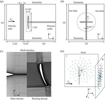
The numerical set-up of a two-bladed propeller ingesting an upstream aerofoil wake is shown in figures 2(a) and 2(b). In the present set-up, the  $x$-axis is along the freestream direction and is the revolving axis of the propeller, the
 $y$-axis is along the spanwise direction of the aerofoil, the
 $z$-axis is perpendicular to the aerofoil, and the coordinate origin is at the centre of the propeller. The revolving phase
 $\varphi$ is defined such that at
 $\varphi =0^\circ$ the propeller is parallel to the aerofoil, at
 $\varphi =90^\circ$ they are perpendicular, and
 $\varphi$ increases with the rotation direction.
(a,b) Schematics of the computational domains and the boundary conditions (not to scale), where the dotted frame and circle denote the boundary of the rotating domain around the propeller. Line 1 in (b) is  $0.1c$ upstream from the propeller disc plane. (c) The coupling interfaces of computational domains. (d) The artificial microphone arrays used in numerical beamforming.

The propeller has diameter  $D=240$ mm, and the upstream NACA 0020 aerofoil has chord length
 $c=100$ mm. The distance from the trailing edge of the aerofoil to the propeller disc plane (
 $x=0$ plane) is
 $0.25c$, which ensures well-built interactions between the wake turbulence and the propeller. Two distinct revolving speeds
 $N$ of the propeller are investigated, i.e. 3000 (with medium thrust) and 4500 (with high thrust) revolutions per minute (rpm), and the freestream speed
 $U_0$ is 5 m s
 $^{-1}$, corresponding to advance ratios
 $J=U_0/ND$ of 0.83 and 0.56, respectively. The Reynolds number based on the freestream velocity and aerofoil chord is
 $Re_c=U_0 c/\nu =3.4\times 10^4$, and the Reynolds number based on the propeller diameter is
 $Re_D=U_0 D/\nu =8.1\times 10^4$, where
 $\nu$ is the kinematic viscosity of the fluid.
The computational domains consist of an outer static domain and an inner rotating domain. Figures 2(a) and 2(b) show the sizes of the domains and the employed boundary conditions. The outer static domain is a rectangular box of length  $7.5D$ in the streamwise direction and length
 $5D$ in the two lateral directions. The inner rotating domain is a cylinder with diameter
 $1.5D$ and height
 $0.15D$. The velocity inlet boundary condition is imposed
 $2.6D$ upstream of the propeller, and the pressure outlet boundary condition is employed
 $5D$ downstream of the propeller. The other four side boundaries are all
 $2.5D$ away from the propeller's centre, where the symmetry boundary conditions are applied in the spanwise direction of the aerofoil, and the far-field boundary conditions are applied to the other two lateral boundaries. The no-slip boundary conditions are prescribed on the surfaces of the propeller and the aerofoil.
The computational mesh is fully structured for both the static domain and the rotating domain, and the mesh interface between the two domains is shown in figure 2(c). For the 3000 rpm case, there are 35 million cells in the rotating domain, and 61 million cells in total. For the 4500 rpm case, there are 39 million cells in the rotating domain, and 66 million cells in total. The wall-adjacent cells are refined to ensure  $y^+<1$ for the first layer and maintain
 ${\rm \Delta} y^+ \sim 1$ for
 $y^+<25$ for each case to resolve the boundary layer accurately.
Wall-resolved large eddy simulations are performed to simulate the propeller wake-ingestion turbulence flow. As the Mach number is less than 0.3 in this work, the spatially filtered incompressible Navier–Stokes equations are solved:
 \begin{equation} \left.\begin{gathered} \frac{\partial \bar{v}_i}{\partial x_i} = 0, \\ \frac{\partial \bar{v}_i}{\partial t} + \frac{\partial \bar{v}_i \bar{v}_j}{\partial x_j} ={-} \frac{1}{\rho}\,\frac{\partial \bar{p}}{\partial x_i} + \nu\, \frac{\partial^2 \bar{v}_i}{\partial x_j\,\partial x_j} - \frac{\partial \tau_{ij}}{\partial x_j}, \end{gathered}\right\} \end{equation}
where an overbar  $\overline {({\cdot })}$ denotes the spatial filter, and
 $\tau _{ij}=\overline {v_i v_j} -\bar {v}_i \bar {v}_j$ is the subgrid-scale stress tensor. The needed subgrid-scale viscosity
 $\nu _{{sgs}}$ is modelled by the Smagorinsky–Lilly model (Smagorinsky Reference Smagorinsky1963)
 \begin{equation} \nu_{{sgs}} = (C_s \varDelta)^2\,|\bar{S}_{ij}|, \end{equation}
where  $C_s=0.1$ is the Smagorinsky constant suggested by van Balen, Uijttewaal & Blanckaert (Reference Van Balen, Uijttewaal and Blanckaert2009) and Yao et al. (Reference Yao, Cao, Wu, Yu and Huang2020),
 $\varDelta$ is the filter width, and
 $\bar {S}_{ij}$ is the filtered strain rate tensor. A standard van Driest damping function (van Driest Reference Van Driest1956) is applied to prescribe
 $\nu _{{sgs}} \rightarrow 0$ near the solid walls.
Figure 2(d) depicts the two multi-armed spiral arrays for the later use of numerical beamforming. Array I is on the side of the propeller, and array II locates downstream of the propeller. Each of the artificial microphone arrays has a distance 0.55 m ( $2.3D$) from the array's centre to the propeller's centre, and consists of 99 virtual microphones to acquire the acoustic pressure.
The acquisition of flow field and acoustic data is performed for 10 revolutions of the propeller after the first 20 revolutions to ensure fully developing of the turbulent flow. The time step corresponds to a  $0.09^\circ$ rotation of the propeller for the 3000 rpm case, and
 $0.135^\circ$ for the 4500 rpm case. At both the microphone arrays and far-field receivers, the radiated noise is computed by solving the aforementioned FW–H equation in (2.8)–(2.10).
3.2. Validation
To ensure the quality of numerical results, a mesh convergence study has been conducted to check the validity of the current computational mesh by comparing with coarse and fine meshes. The coarse mesh has 36 million cells in total, and 21 million in the rotating domain, and the fine mesh has 108 million cells in total, and 59 million cells in the rotating domain.
Figure 3(a) compares the phase-averaged axial velocity on Line 1, which is shown in figure 2(b), across different grid refinements. Unless specifically mentioned, the phase average in this paper is performed by averaging over the values at fixed revolving phases. The medium and fine meshes give similar distributions of the axial velocity, while the result of the coarse mesh shows velocity mismatch near  $z=0$. Figure 3(b) compares the phase-averaged axial force of the propeller. The result of the medium mesh is close to that of the fine mesh, and the coarse mesh underestimates the force by 10 %. Given that the differences in the results between the medium grid refinement of 61 million and the fine grid refinement of 108 million are less than 2 % for the majority of the phase angles, we chose the medium grid refinement in the subsequent numerical studies. Moreover, the simulations are validated by comparing the numerical results with the measured data from previous PIV experiments conducted by Chen et al. (Reference Chen, Peng, Liem and Huang2020a). Figure 4 compares the axial velocity distribution on Line 1. Both the results are phase-averaged at three revolving phases,
 $-9^\circ$,
 $0^\circ$ and
 $9^\circ$, which correspond to the propeller's three representative stages of entrance into, cutting through and departure from the wake region. The results in figure 4 show good agreement between the experiments and the present numerical results. The velocity profiles are well captured, and the amplitude discrepancy is within 10 % for most of the points on the lines.
(a) The mean axial velocity on Line 1, and (b) the axial force of the propeller, predicted with different grid refinements. The revolving speed is 3000 rpm.

Measured and simulated mean velocity on Line 1 (see figure 2b) at the revolving phases (a)  $\varphi =-9^\circ$, (b)
 $\varphi =0^\circ$, and (c)
 $\varphi =9^\circ$. The revolving speed is at 4500 rpm. The measured flow field data are from Chen et al. (Reference Chen, Peng, Liem and Huang2020a).

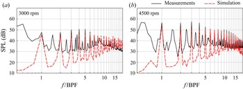
Figure 5 compares the computed and measured far-field sound pressure level (SPL) values, both of which are averaged over 56 microphones to reduce the potential interference. The background noise of the wind tunnel is subtracted from the measured results by subtracting the corresponding acoustic energy at each frequency. Strong peaks are found at the BPF and its harmonics, which is a distinctive feature of this wake-ingestion set-up. The peaks at half-BPF and its harmonics in the measurements are caused by the asymmetry blade–rotor interaction and the imperfect blade geometry (Wu et al. Reference Wu, Jiang, Ma, Chen and Huang2022), which is not modelled in the current numerical simulations and therefore results in discrepancies at the half-BPF and its harmonics in figure 5.
Measured and simulated sound pressure levels at the revolving speeds (a) 3000 rpm and (b) 4500 rpm. The measured sound data are from Chen et al. (Reference Chen, Peng, Liem and Huang2020a).

The comparison with measured results shows good agreement around the BPF harmonics. The difference between simulated noise and the measurements at the first two harmonics of the BPF is less than 3 dB. At the next few BPF harmonics, the differences are within 5 dB. Due to the upstream turbulent flow in the wind tunnel, the measured broadband noise is louder than the simulation at low to mid frequencies. In summary, the current simulation set-ups and numerical schemes are validated by the measurements; the calculated flow field results will be used below for the near-field noise source analysis.
3.3. Flow characteristics
To provide a more comprehensive perspective on the wake-ingestion problem, the flow characteristics are first introduced. Figure 6(a) shows the instantaneous flow structures at 3000 rpm by plotting isosurfaces of the  $Q$-criterion (Haller Reference Haller2005) that are coloured by the normalized vorticity. Four kinds of structures are denoted:
 ${\unicode{x2460}}$ denotes the tip vortices that are generated by the pressure difference between the pressure side and suction side of the propeller blades;
 ${\unicode{x2461}}$ denotes the trailing edge shedding vortices of the propeller blades;
 ${\unicode{x2462}}$ denotes the root vortices; and
 ${\unicode{x2463}}$ denotes the shedding vortex from the upstream aerofoil.
(a) Flow structures at 3000 rpm shown by isosurfaces of  $Q(R/U_0)^2=10$ and coloured by
 $\omega _z R/U_0$. Here,
 ${\unicode{x2460}}$ indicates the blade tip vortex,
 ${\unicode{x2461}}$ the blade trailing edge vortex,
 ${\unicode{x2462}}$ the rotor root vortex, and
 ${\unicode{x2463}}$ the aerofoil shedding vortex. (b) Contours of instantaneous radial vorticity
 $\omega _r R/U_0$ at 3000 rpm on cylindrical surfaces
 $r/R=0.25$ (inner) and
 $r/R=0.75$ (outer) at phase angle
 $\varphi =0^\circ$.

Figure 6(b) shows the instantaneous radial vorticity of the flow field at 3000 rpm on the  $r/R=0.25$ and
 $r/R=0.75$ cylindrical surfaces at
 $\varphi =0^\circ$, where
 $r$ denotes the local radius to the revolving axis. In addition to the vorticity of the aerofoil wake, the trailing edge vortex shedding of the blade is shown clearly on the surface at
 $r/R=0.75$. However, due to the smaller radius and lower relative velocity, the trailing edge vortex shedding is not observed on the surface at
 $r/R=0.25$.
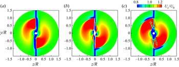
The phase-averaged axial velocities at the blade leading edge plane ( $x/R=-0.05$), rotor midplane (
 $x/R=0$) and blade trailing edge plane (
 $x/R=0.05$) are given in figure 7. It is clear that the aerofoil wake resulted in the low-velocity band in the middle of the plane, while the rotation of the blade accelerates the flow and leaves the high axial velocity region behind the blade. At the rotor mid-plane and blade trailing edge plane, a low-velocity band above the blade tip can be seen, which is the result of the blade tip vortex. At the blade trailing edge plane, the centre low-velocity region is due to the blade hub, and the thin low-velocity band lagging behind the blade is due to the trailing edge vortex shedding.
Phase-averaged axial velocity on different cross-sections: (a)  $x/R=-0.05$, (b)
 $x/R=0$, and (c)
 $x/R=0.05$. The propeller rotates in the clockwise direction.

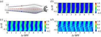
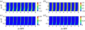
The wake–rotor interaction process can be demonstrated by the correlation of pressure fluctuations, which is analysed on the suction surface for three sample lines from leading edge to trailing edge at 10 %, 50 % and 90 % local chord, as shown in figure 8(a). The space–time correlation coefficients of pressure fluctuations  $C_{p^\prime p^\prime }(0.6R,{\rm \Delta} r,{\rm \Delta} t)$ for the base points at
 $r/R=0.6$ to other points on the same sample lines are plotted in figures 8(b)–8(d), and the correlation coefficient is defined as (Wang et al. Reference Wang, Wang and Wang2021)
 \begin{equation} C_{p^\prime p^\prime}(r,{\rm \Delta} r,{\rm \Delta} t) = \frac{\langle p^\prime(r,t)\,p^\prime(r,r+{\rm \Delta} r,t+{\rm \Delta} t) \rangle}{\sqrt{\langle p^\prime(r,t) \rangle^2}\, \sqrt{\langle p^\prime(r,r+{\rm \Delta} r,t+{\rm \Delta} t) \rangle^2}}, \end{equation}
where  $\langle {\cdot } \rangle$ denotes time averaging.
(a) Sample lines on the suction side of the blade surface. Solid line is 10 % local chord; dashed line is 50 % chord; dash-dotted line is 90 % chord. The solid circles denote the  $r/R=0.6$ points on each line. (b–d) Space–time correlation coefficients of the pressure fluctuations
 $C_{p^\prime p^\prime }(0.6R,{\rm \Delta} r,{\rm \Delta} t)$ on (b) 10 %, (c) 50 % and (d) 90 % chord sample lines.

It is observed that the correlation coefficients on all three sample lines show a periodic pattern, and the high values align with the aerofoil wake-cutting timing. The bias of the high correlation coefficient to the left near  ${\rm \Delta} r/R=-0.3$ is due to the fact that the blade at
 $r/R=0.3$ enters the wake of the aerofoil earlier than the rest of the blade due to the bumped geometry. Figures 8(b)–8(d) also show that the correlation is stronger for the lines closer to the leading edge, which indicates that the wake-cutting effect and the generated fluctuations decay from leading edge (LE) to trailing edge (TE).
Figures 9(a) and 9(b) show the blade-to-blade space–time correlation coefficient  $C_{p^\prime p^\prime }(0.6R,{\rm \Delta} r,{\rm \Delta} t)$, where the base point and the correlated points are both at the 10 % chord sample line but on two different blades. Due to the symmetrical set-up of the wake-ingesting configuration, the blade-to-blade correlations are very similar to the correlations of the same blade. Moreover, the correlation coefficient of the 4500 rpm case is higher than that of the 3000 rpm case, which was also observed in the work of Wang et al. (Reference Wang, Wang and Wang2021).
(a,b) Blade-to-blade correlation coefficient of the pressure fluctuations  $C_{p^\prime p^\prime }(0.6R,{\rm \Delta} r,{\rm \Delta} t)$ between two different blades for (a) 3000 rpm and (b) 4500 rpm on the 10 % chord sample line. (c,d) Space–time correlation coefficient of the time derivative of the pressure
 $C_{\dot {p} \dot {p}}(0.6R,{\rm \Delta} r,{\rm \Delta} t)$ for (c) 3000 rpm and (d) 4500 rpm on the 10 % chord sample line.

Figures 9(c) and 9(d) plot the correlation coefficient of the time derivative of the pressure  $C_{\dot {p} \dot {p}}(0.6R,{\rm \Delta} r,{\rm \Delta} t)$ defined in the same way as in (3.3) for 3000 and 4500 rpm cases at the 10 % chord sample line. Similar to the correlation coefficient of the pressure fluctuations, the
 $C_{\dot {p} \dot {p}}(0.6R,{\rm \Delta} r,{\rm \Delta} t)$ level changes periodically with the rotation, and the high value corresponds to the wake-cutting process. The correlation of the time derivative of the pressure is weaker than that of pressure fluctuations because the time derivative puts more weight on high-frequency components, while the correlated sources at leading edge are mainly at lower frequencies.
4. Acoustic imaging analysis
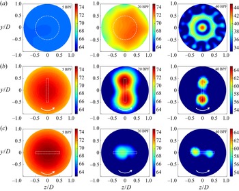
First, the noise sources are investigated using the numerical beamforming approach. Figure 10 presents the acoustic imaging results on the propeller disc plane, by applying separately the classical beamforming and the wavelet-based beamforming to the wake-ingestion flow of the propeller at the revolving speed 3000 rpm. The microphone array II shown in figure 2 is used to produce the acoustic imaging results. Three representative frequencies are investigated to cover low to high frequencies, which correspond to 5 BPF, 20 BPF and 40 BPF, respectively. The dynamic range of all the acoustic imaging results is set to 12 dB.
Beamforming results on the propeller disc plane ( $x=0$). The imaging results are obtained by (a) classical beamforming, and (b,c) wavelet-based beamforming. For wavelet-based beamforming results, the revolving phase is at (b)
 $\varphi =0^\circ$, and (c)
 $\varphi =90^\circ$. In (a), the dashed circles denote the trajectory swept by the blade tip. In (b,c), the dashed frames denote the instantaneous propeller projection. The propeller rotates at speed 3000 rpm in the anticlockwise direction, as denoted by the arrow.

Figure 10(a) shows the imaging results of classical beamforming, where the dashed circles represent the trajectory swept by the propeller's blade tip in one revolution. The source maps for low (the left-hand plot in figure 10a) and mid (the middle plot) frequencies are too unrecognizable to identify clearly the possible aeroacoustic source locations. At the highest frequency, the source map suggests that the sources are mainly around the blades’ root and tip, which collectively form a concentrated point source in the centre of the propeller and a circular distributed source at the outer rim of the blades’ revolution trajectory. Figure 10(a) shows that the classical beamforming provides only time-averaged results, and sources at different phases are superimposed together, making it not so suitable to localize phase-dependent noise sources.
Next, the recently developed wavelet-based beamforming technique is adopted to reconstruct the time-varying aeroacoustic sources from the computational fluid dynamic solutions. Figures 10(b) and 10(c) exhibit the imaging results obtained at two representative revolving angles by using wavelet-based beamforming. The dashed frames denote the projections of the propeller on the disc plane at the corresponding angles. The wavelet-based beamforming results are phase-averaged over 10 revolutions to reduce random interferences. The low-frequency imaging results at  $f=5$ BPF suggest that at
 $\varphi =0^\circ$, the noise radiation is louder than that at
 $\varphi =90^\circ$ by more than
 $10\,$dB. This comparison demonstrates clearly that the dominant noise sources are from the interaction between the turbulent wake and the propeller, which occurs at
 $\varphi =0^\circ$, and the corresponding aeroacoustic sources show strong dependency on the revolving phase. Nevertheless, the low resolution of imaging results at low frequency (left-hand plots in figures 10(b) and 10(c)) still makes it impossible to identify clearly the location of the noise sources.
The mid frequency results for  $f=20$ BPF also indicate that the noise sources are dominant at
 $\varphi =0^\circ$ when the blades are interacting with the wake. Compared to the left-hand plots in figure 10, the imaging resolution of the middle plots is slightly improved, such that the sources are found to be in the proximity of the blades, and is more significant at the outer half of the blades around
 $0.7R$. Figure 5(b) shows the high-frequency imaging results of the aeroacoustic sources. Unlike the imaging results at the two lower frequencies, the high-frequency sources for
 $f=40$ BPF at
 $\varphi =0^\circ$ are slightly louder than those at
 $\varphi =90^\circ$ by 3 dB. Moreover, at this high frequency, the resolution of the aeroacoustic source maps is much refined, and the sources that distribute from the tip to the outer half of the blades can be recognized clearly.
Figure 11 illustrates the noise sources obtained from wavelet-based beamforming for the 4500 rpm case on different planes. Figures 11(a) and 11(b) show the results on the  $x=0$ plane, and figure 11(c) shows the results on the
 $z=0$ plane. The images are phase-averaged, and the frequencies 5 BPF, 20 BPF and 40 BPF are investigated.
Wavelet-based beamforming results on (a,b) the propeller disc plane ( $x=0$), and (c) the
 $z=0$ plane. The revolving phase is at (a,c)
 $\varphi =0^\circ$ and (b)
 $\varphi =90^\circ$, and the revolving speed is at 4500 rpm. Other set-ups are the same as those in figure 10.

The results of figures 11(a) and 11(b) are similar to those in figures 10(b) and 10(c). Due to the wake interaction at  $\varphi =0^\circ$, the aeroacoustic sources of low and mid frequencies are significantly stronger than those at
 $\varphi =90^\circ$. The high-frequency sources are almost the same at both revolving phases. The resolution in the right-hand plots of figures 10 and 11 has been further refined thanks to the higher frequency, thus showing that high-frequency sources are near the trailing edge of the blades with a distance to the revolving axis between
 $0.6R$ and
 $0.8R$.
Figure 11(c) shows the wavelet-based beamforming results on the  $z=0$ plane at phase
 $\varphi =0^\circ$. As beamforming lacks the resolution in the perpendicular direction to the array plane, these new results with array II (see figure 2) can provide source distribution in the
 $x$ direction. The low-frequency sources are mainly over the blade tips, while the mid- and high-frequency sources appear at the blade mid-span.
The above acoustic imaging results clearly demonstrate that the aeroacoustic source varies with the rotating motion of the blades. The dominant noises at low to mid frequencies are highly correlated to the wake–rotor interactions, while the dominant noises at high frequencies near the trailing edge are more likely to arise from the propeller itself, e.g. the trailing edge vortex shedding observed in figure 6.
However, the current imaging results also show that the resolution of the numerical beamforming does not suffice to localize the distribution of sources on the propeller surface for design improvement or noise evaluation and control. The beamforming resolution limit is fundamentally subject to the frequencies of the interested noise and the array aperture (Chen, Zhong & Huang Reference Chen, Zhong and Huang2020b), which is inherent in its theory. To address this issue, the near-field aeroacoustic sources analysis approach introduced in § 2 is applied to investigate further the noise sources.
5. Near-field aeroacoustic sources analysis
A comprehensive noise sources study has been executed following the near-field aeroacoustic sources analysis approach. First, the contribution of thickness noise sources ( $\boldsymbol {S_T}$) and loading sources (
 $\boldsymbol {S_{L1}},\boldsymbol {S_{L2}}$) to the far-field noise was investigated. Then the on-surface noise distribution was presented and correlated to the flow features, followed by the discussion of sources at different phases and their spectra at different blade locations. Finally, different noise identification methods were compared and discussed.
5.1. Contribution of noise sources
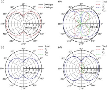
Figure 12(a) shows the directivity of overall sound pressure level (OASPL) at far-field receivers  $400D$ away from the propeller centre on the
 $y=0$ plane, which are far enough away to neglect the near-field effects. The directivity angle
 $0^\circ$ denotes the downstream direction with the receiver at
 $(400D, 0,0)$, and the directivity angle increases anticlockwise. The OASPL of the noise at the receiver is calculated by
 \begin{equation} \text{OASPL} = 10 \log_{10}\int \frac{\phi_{pp}(f)}{p^2_{{ref}}}\,{\rm d} f, \end{equation}
where  $\phi _{pp}(f)$ is the power spectral density, and the integration is performed in the frequency range from
 $25\,\textrm {Hz}$ to
 $8000\,\textrm {Hz}$. The directivity results show that the radiated noise is strongest in the upstream and downstream directions, and is relatively weak on the propeller disc plane, which is also observed in other propeller studies with the ingestion of an upstream turbulent wake (Wang et al. Reference Wang, Wang and Wang2021). Figure 12(a) shows that dipole-type directivity patterns at 3000 and 4500 rpm are almost the same, and the OASPL increases with the revolving speed.
Directivity of the noise at far-field receivers on the  $y=0$ plane. (a) OASPL of the total noise. (b) Contribution of each noise source component at the BPF with 4500 rpm. (c) OASPL of the noise source components at 3000 rpm. (d) OASPL of the noise source components at 4500 rpm.

Figures 12(b)–12(d) compare the contribution of each noise source term to the far-field noise, where the thickness source term  $\boldsymbol {S}_{T}$ and the two loading source terms
 $\boldsymbol {S}_{L1}$ and
 $\boldsymbol {S}_{L2}$ are defined in (2.15). The directivity of noise contributions from the three components are evaluated at far-field receivers that are the same as those used in figure 12(a). Figure 12(b) shows the contributions of each noise component at BPF for the 4500 rpm case. At the BPF, the thickness noise from
 $\boldsymbol {S}_{T}$ is dominant in the
 $90^\circ$ (above the propeller) and
 $270^\circ$ (under the propeller) directions, and has a shape of ‘
 $\infty$’. The noise from
 $\boldsymbol {S}_{L1}$ is loudest in the
 $0^\circ$ (upstream) and
 $180^\circ$ (downstream) directions, and is dominant in most directions. The noise from
 $\boldsymbol {S}_{L2}$ reaches its peak around
 $60^\circ$ and
 $300^\circ$, and decreases greatly in other directions. By comparison,
 $\boldsymbol {S}_{L2}$ is much weaker than the other two source terms. The results agree well with the theoretical discussions in § 2.2. The only exception is that the noise from
 $\boldsymbol {S}_{L2}$ is more than expected in the directions from
 $60^\circ$ to
 $90^\circ$ and from
 $270^\circ$ to
 $300^\circ$, where it is comparable or even louder than the noise from
 $\boldsymbol {S}_{L1}$. The reason for this is that although stronger sound sources could produce a louder noise, they can also possibly cancel each other in certain directions, making the resulting noise less loud than expected at those angles.
Figures 12(c) and 12(d) demonstrate the OASPL of each noise component for the 3000 and 4500 rpm cases, respectively. The OASPL results include higher-frequency noise, and  $\boldsymbol {S}_{L1}$ generates larger overall noise than the other two source terms. At 3000 rpm, the noise contributions from
 $\boldsymbol {S}_{T}$ and
 $\boldsymbol {S}_{L2}$ are too small to be shown. As the thickness noise is related directly to the revolving speed,
 $\boldsymbol {S}_{T}$ at 4500 rpm is around 15 dB larger than at 3000 rpm. And the noise from
 $\boldsymbol {S}_{L2}$ at 4500 rpm is around 18 dB larger than at 3000 rpm.
Figure 13 demonstrates a snapshot at phase  $\varphi =0^\circ$ for the contributions of each surface computational element on the blade suction side to the noise at downstream receiver
 $(400D,0,0)$ and above the propeller receiver
 $(0, 400D,0)$. For each surface element, the contributions are calculated by the quantities inside the integrals in (2.12) and (2.13), which are labelled as thickness, loading 1 and loading 2, corresponding to the aeroacoustic sources
 $\boldsymbol {S}_T$,
 $\boldsymbol {S}_{L1}$ and
 $\boldsymbol {S}_{L2}$, respectively. The contributions are divided by the element area
 $\mathrm {d}S$ and evaluated at the receiver time, so that the noise signal of the receiver can be calculated by summing the product of the contribution and area of each surface element. Negative and positive contributions are represented by the blue and red colours, respectively. The coexistence of negative and positive contributions would lead to the aforementioned cancellation at the far-field receivers in figure 12.
A snapshot of the contribution to far-field noise at two receivers by the surface elements on the suction side of the propeller blades. From top to bottom, rows are the elementary contributions from  $\boldsymbol {S}_T$,
 $\boldsymbol {S}_{L1}$,
 $\boldsymbol {S}_{L2}$ and the total acoustic pressure, respectively. The left side is for the downstream receiver at
 $(400D,0,0)$, and the right side is for the receiver above the propeller at
 $(0,400D,0)$.

It is clear that the contributions from the source terms to different receivers are different. For the downstream receiver, the contributions from the thickness noise and  $\boldsymbol {S}_{L2}$ are nearly invisible, and the total contribution is almost the same as that from
 $\boldsymbol {S}_{L1}$. This means that the noise in the downstream direction is dominated by the
 $\boldsymbol {S}_{L1}$ source, which agrees with the directivity patterns in figure 12. For the receivers above the propeller, the contribution from thickness noise
 $\boldsymbol {S}_{T}$ and loading noise
 $\boldsymbol {S}_{L2}$ becomes more distinctive, although the total contribution still remains largely dependent on
 $\boldsymbol {S}_{L1}$. The results of surface element contributions support the observation that
 $\boldsymbol {S}_{L1}$ is the major acoustic source for the current physical problem studied, and justify the choice of
 $\boldsymbol {S}_{L1}$ as the focus of discussion in most of the following subsections.
5.2. On-surface source distributions
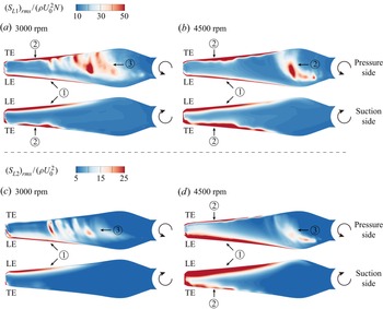
Figure 14 shows the surface distribution of the r.m.s. value of the normalized loading noise sources, i.e.  $(S_{L1})_{{rms}}/(\rho U_0^2 N)$ and
 $(S_{L2})_{{rms}}/(\rho U_0^2)$. The time average is implemented for 10 revolutions, and the results show the average of the sources at all phases. The abbreviations ‘LE’ and ‘TE’ in figure 14 stand for leading edge and trailing edge, respectively. For the distribution of
 $(S_{L1})_{{rms}}$, strong sources are found in three regions that are classified and noted by the markers in figure 14, where:
 ${\unicode{x2460}}$ denotes the sources at the leading edge that appear on both sides of the blade, which is due to the interaction between the propeller blades and the ingesting wake;
 ${\unicode{x2461}}$ denotes the sources at the trailing edge of the blade, which is also observed on both sides of the blades; and
 ${\unicode{x2462}}$ denotes the sources that are found only in the middle section of the pressure side of the blade. The other surface area covered in blue colour indicates weaker sources.
The amplitude of the loading noise sources (a,b)  $(S_{L1})_{{rms}}/(\rho U_0^2 N)$ and (c,d)
 $(S_{L2})_{{rms}}/(\rho U_0^2)$ on the propeller surface. The revolving speed is (a,c) 3000 rpm and (b,d) 4500 rpm. The abbreviations ‘LE’ and ‘TE’ stand for leading edge and trailing edge, respectively.

The distributions are generally similar for both revolving speeds. At the higher rpm speed, the leading edge and trailing edge sources are stronger, manifesting a positive relation between on-surface aeroacoustic sources and the far-field noise emission. However, the pressure side mid-span sources are stronger at 3000 rpm. This is because the relative angle of attack (AoA) is larger at lower revolving speeds leading to stronger separation when the incoming mean flow is fixed at  $U_0$.
In figures 14(c) and 14(d), the secondary loading source  $(S_{L2})_{{rms}}$ presents distributions similar to those of
 $(S_{L1})_{{rms}}$. A distinctive distribution of sources can also be found at the leading edge, trailing edge and mid-span of the blade pressure side. It should be noted that the value of
 $S_{L2}$ is lower compared to
 $S_{L1}$ and plotted with different scales. At the trailing edge, the source of
 $(S_{L2})_{{rms}}$ is absent at 3000 rpm on the suction side.
In § 2, it has been discussed that the loading sources are affected by the background flow. This is particularly true for the current turbulent ingestion propeller problem, which contains the direct interaction between the upstream shedding vortex and the downstream propeller blades. Pressure fluctuations are produced near the leading edge as the blade cuts through the shedding vortex of the aerofoil generating the leading edge sources. Figure 15 demonstrates the interaction procedure at several different revolving phases on the cross-section plane at the radial height  $0.5R$, where
 $R$ is the radius of the blade. The normalized vorticity
 $\omega _y R/U_0$ perpendicular to the plane is plotted to reflect the flow interaction procedure. At
 $\varphi =-9^\circ$, the propeller blade is about to enter the wake region, and the leading edge of the blade has just cut into the shedding vortex of the aerofoil. At
 $\varphi =0^\circ$, the blade cuts and separates the shedding vortex into two parts, resulting in the discontinuity of the wake of the aerofoil. At
 $\varphi =9^\circ$, the blade is leaving the wake region, and at the downstream to the blade, the shedding vortex of the aerofoil is slightly brought upwards due to the shear force from the blade. The shedding vortex of the blade itself is also left behind and would further interact with the wake of the upstream aerofoil.
Evolution of the vortices on the cross-section plane at the radial height  $0.5R$ at phases (a)
 $\varphi =-9^\circ$, (b)
 $\varphi =0^\circ$, and (c)
 $\varphi =9^\circ$. The vorticity is normalized to
 $\omega _y R/U_0$. The current revolving speed is 3000 rpm.

Apart from the interaction, the rotating motion has also led to flow mechanisms that generate noise sources. Figure 16 exhibits snapshots of the static pressure coefficients  $C_p$ at phase angle
 $\varphi =0$ on four section planes with radial heights
 $0.25R$,
 $0.5R$,
 $0.75R$ and
 $R$. Near the blade leading edge, the stagnation points have moved slightly rearward on the suction side because of the negative relative AoA. More specifically, the relative AoA is defined by
 $\mathrm {AoA}_{{rel}}=\theta _r-\mathrm {atan}(U_0/2{\rm \pi} N r_s)$, where
 $\theta _r$ is the pitch angle between the chord line and the
 $z$-axis, and
 $r_s$ is the radial height of the section plane. The corresponding
 $\mathrm {AoA}_{{rel}}$ values at
 $0.25R$,
 $0.5R$ and
 $0.75R$ are
 $-8^\circ$,
 $-2^\circ$ and
 $-1^\circ$, respectively.
Pressure coefficients on several section planes at phase  $\varphi =0^\circ$. The section plane has a distance to the revolving axis (a)
 $0.25R$, (b)
 $0.5R$, (c)
 $0.75R$, and (d)
 $R$. The current revolving speed is 3000 rpm.

On the section plane of  $r_s=0.25R$, the negative
 $\mathrm {AoA}_{{rel}}$ leads to the adverse pressure gradient close to the pressure side of the blade. At increased distances to the rotation axis
 $0.5R$ and
 $0.75R$,
 $\mathrm {AoA}_{{rel}}$ increases and the flow on the pressure side shows less adverse pressure gradient, and the suction side would become more normal in terms of the pressure gradient. At
 $r_s=R$, which is over the blade tip, the pressure difference between the pressure and suction sides would lead to the generation of a tip vortex.
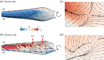
Figure 17 shows the phase-averaged limiting streamlines on the propeller blade over the distribution of phase-averaged static pressure coefficients. The phase average is implemented by averaging over the results at the same revolving phase  $\varphi$ for more than 10 revolutions to ensure statistical confidence. Only the result at 3000 rpm is presented for brevity, since the higher revolving speed case has a similar pressure distribution and streamlines. The pressure difference between the suction and pressure sides is larger at the outer half of the blade, suggesting that the lift is mostly generated therein. The negative pressure gradient at the leading edge and trailing edge on the pressure side is observed.
Phase-averaged limiting streamlines and pressure coefficients on the propeller blade at phase  $\varphi =0^\circ$. (a,b) Phase-averaged static pressure distributions overlapped with limiting streamlines. (c,d) Close views of limiting streamlines on the pressure side of the blade. The current revolving speed is 3000 rpm.

The limiting streamline is obtained from the wall shear stress that is computed from the relative velocity. Generally, the flow on the suction side of the blade is smooth, except for the gathering of streamlines near the trailing edge that drives the fluid towards the blade tip. The reversed streamlines from the trailing edge to the gathering line indicate flow separation near the trailing edge, which is a potential cause of noise sources. On the pressure side, however, the streamlines reflect complicated flow patterns in the boundary layer. The aggregated streamlines near the leading edge reveal the movement from the root half of the blade to different destinations, including the leading edge, the trailing edge of the tip half, and other places of the blade. Moreover, on the pressure side, the streamlines from the root to the middle part indicate the existence of complicated patterns that are further illustrated in the enlarged views in figures 17(c) and 17(d), where the nodal and saddle points can be identified by following the definitions from Tobak & Peake (Reference Tobak and Peake1982). Flow separations and interactions occur at these spots, which lead to the aeroacoustic sources.
5.3. Sources at different phases
Due to the unsteady flow interaction between the spatially non-uniform wake and the propeller, the distribution of on-surface aeroacoustic sources varies along with the revolving phases. Figure 18 presents an overview of the relationship between on-surface sources and the flow phenomenon for a single blade at various revolving phases. The shedding vortices separated from the aerofoil and the propeller blade on two section planes at  $0.3R$ and
 $0.6R$ radial heights are shown by rainbow-scale colours. Only the 4500 rpm case is presented for brevity; the results at 3000 rpm are similar in distribution.
Variations of on-surface aeroacoustic sources as a single blade of the propeller rotates and interacts with the ingesting wake flow. The red–blue colour on the surface of the blade denotes the amplitude of the loading noise source  $\boldsymbol {S_{L1}}$. The rainbow scale in the field denotes the normalized vorticity
 $\omega _y R/U_0$. The surface sources are phase-averaged, superimposed for the single blade at 12 representative rotating angles from
 $0^\circ$ to
 $360^\circ$, while the vorticity plot is a snapshot when
 $\varphi =0^\circ$. The revolving speed of the propeller is 4500 rpm.

At phases  $0^\circ$ and
 $180^\circ$, where the blade is cutting through the wake of the aerofoil, figure 18 shows that strong aeroacoustic sources are generated at the leading edge of the blade. At other revolving phases, the leading edge noise sources are less prominent, which reflects the direct relationship between the leading edge sources and the interaction between the ingesting wake and the blade. On the contrary, noise sources at the trailing edge persist at a certain strength at each revolving phase, suggesting that they are less correlated to the wake-ingestion.
To have a more detailed view of the interaction process, figure 19 shows the aeroacoustic sources on the blade suction side over various revolving phases by smaller revolving steps. During the interaction procedure, the leading edge sources grow stronger from  $-15^\circ$ to
 $0^\circ$; at
 $-15^\circ$, the leading edge sources barely exist at the root half blade, which has already entered into the wake region, whereas the tip half blade is still outside the wake region; when the blade moves further into the wake region, the aeroacoustic sources grow stronger and finally reach the peak at
 $0^\circ$. Then the sources become gradually weaker; at
 $5^\circ$, the leading edge source is still evident, while at
 $10^\circ$ and later revolving phases, the aeroacoustic sources are almost absent at the leading edge. In contrast, the trailing edge aeroacoustic sources are less affected by the interaction, and their distribution over the blade remains nearly the same over the whole interaction procedure.
Amplitude of the aeroacoustic source  $S_{L1}$ on the blade suction side at various revolving phases from
 $-15^\circ$ to
 $15^\circ$. The revolving speed is 4500 rpm.

The aeroacoustic sources associated with the wake impingement are revealed in figure 19. In particular, when the revolving phase is between  $5^\circ$ and
 $10^\circ$, a vertical strip that represents strong sources appears at the middle of the blade surface, which is the result of the wake impingement. Additionally, the proposed approach helps to show the location of the impingement that moves from the leading edge to the trailing edge as the blade rotates through the wake region.
Figure 20 shows the on-surface aeroacoustic sources on the pressure side of the blade. The variation of the leading and trailing edge sources along with the revolving phase is similar to the results in figure 19. The mid-span sources, which are observed only on the pressure side, preserve a similar distribution at different phases. This is consistent with the observation that the mid-span sources are created mainly by the complicated local flows rather than the wake interaction process as discussed in § 5.2. Moreover, since the direct wake impingement occurs only on the upstream-facing suction side, the effect of impingement is not observed on the pressure side.
Amplitude of the aeroacoustic source  $S_{L1}$ on the blade pressure side. Other set-ups are the same as those in figure 19.

5.4. Sources at different frequencies
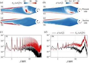
The frequency properties of the aeroacoustic sources are discussed in this subsection. Figure 21 compares the amplitude of the aeroacoustic source at several representative points on the blade surface to illustrate the frequency-domain properties. As shown in figure 21(a), the points are on the section plane at radius  $0.6R$, of which P1–P4 are on the suction side, and P5–P8 are on the pressure side. Figure 21(b) illustrates further the locations of the points on the blade section; in particular, P1 and P8 are at the leading edge, and P4 and P5 are at the trailing edge.
Spectra of  $S_{L1}$ at various surface points. (a,b) Locations of the points of interest. (c,d) Spectra at 3000 rpm. (e,f) Spectra at 4500 rpm.

Figures 21(c)–21(f) show that the distinctive peaks of the spectral results of  $S_{L1}(f)$ are at the BPF and its harmonics. At the leading edge points (P1 and P8) those peaks have the highest values, and become gradually lower at points further downstream, which indicates the weakening of the wake interaction effects moving from leading edge to trailing edge on the propeller surfaces. Moreover, at the trailing edge points (P4 and P5), steep humps appear at high frequencies, which indicates the rise of a high-frequency noise source.
The spectra present certain differences in the shape and amplitude at the two revolving speeds. At 4500 rpm, the peak values at the BPF and its harmonics are higher, which manifests a stronger interaction at higher speeds. While the broadband values do not show much difference, the hump appears at a higher frequency in the 4500 rpm case. The peak value of the hump is also much higher, which would result in a louder noise emitting from the trailing edge.
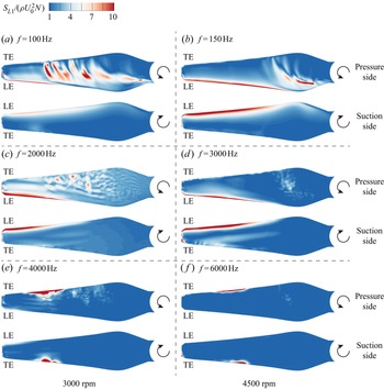
Figure 22 shows the distribution of surface sources at different frequencies. The frequency-domain source  $S_{L1}(\boldsymbol {x},f)$ is calculated by directly taking a Fourier transform to the time-domain source amplitude
 $S_{L1}(\boldsymbol {x},t)$. Although the frequency of the source does not coincide exactly with the frequency of the far-field noise due to the Doppler effect, the frequency-domain results can still be used to isolate surface sources of different frequencies.
Distribution of normalized sources  $S_{L1}$ at various frequencies. The frequencies BPF, 20 BPF and 40 BPF are investigated. The revolving speed is (a,c,e) 3000 rpm, and (b,d,f) 4500 rpm.

Three representative frequencies are compared, i.e. BPF, 20 BPF and 40 BPF in each case. Unlike the beamforming results shown in figures 10 and 11, the on-surface aeroacoustic sources have a resolution as high as the computational mesh, and the distribution of sources at each frequency is shown clearly. At the BPF, strong sources appear at the leading edge on both the pressure and suction sides, and also in the middle of the blade's pressure side. At the mid frequency 20 BPF, the most significant sources are still at the leading edge, while the mid-span sources are weaker. At the higher frequency, significant sources appear only at the trailing edge with radius from  $0.5R$ to
 $0.8R$, indicating a shift from the leading edge noise to the trailing edge noise. The locations of the high-frequency source coincide with the high-frequency imaging results in figures 11(a) and 11(b) at both revolving speeds.
The source distributions are similar under the two revolving speeds. The mid-span sources on the pressure side at 3000 rpm cover a larger area due to the complex flows and separation caused by the large negative  $\mathrm {AoA}_{{rel}}$. With regard to source strength, the leading edge noise sources at BPF and 20 BPF are much stronger at 4500 rpm, which agrees with the far-field noise and beamforming results.
5.5. Comparison of source analysis methods
In the above study, the propeller wake-ingesting noise has been analysed comprehensively using the near-field aeroacoustic source approach. A comparison with other source identification methods, such as surface pressure fluctuations visualization and numerical beamforming, would show their strengths and limitations.
As reviewed in § 1, the surface pressure fluctuation  $p^\prime =p-p_0$ has been used in many previous works to represent the aeroacoustic sources, where
 $p_0$ is the time-averaged pressure. A Fourier transform of the time derivative of the pressure gives
 $\mathcal {F}(\dot {p}) = 2{\rm \pi} \textrm {i}f\,\mathcal {F}(p)$. As a result, in the proposed source model
 $\boldsymbol {S_{L1}}$, its high-frequency components are less likely to be overwhelmed by low-frequency components. Hence, as shown below, fine-scale structures usually remain in the near-field distribution of aeroacoustic sources when the proposed source model approach is adopted.
Figures 23(a) and 23(b) compare the surface distributions of the r.m.s. of the proposed source  $S_{L1}$ and pressure fluctuations
 $p^\prime$. The distributions at the leading edge are similar, but the noise source at the trailing edge in the
 $p^\prime$ plot is not as evident as that in
 $S_{L1}$ plot. This is due to the fact that trailing edge noises are mostly high-frequency sources, as has been discussed in § 5 and figure 22. Also, the sources in the middle of the blade pressure side show differences.
Amplitude of (a) loading noise sources  $(S_{L1})_{{rms}}$ and (b) pressure fluctuations
 $p^\prime _{{rms}}$ on the propeller surface. (c,d) Spectra at P1 and P4, respectively. The revolving speed is 4500 rpm.

Figures 23(c) and 23(d) compare the spectra of  $S_{L1}$ and
 $p^\prime$ at two points on the suction side of the blade, i.e. P1 and P4 in figure 21. At the leading edge point (P1), the amplitudes of
 $S_{L1}$ and
 $p^\prime$ at the BPF and its first few harmonics are close, while the broadband component and harmonic components of
 $S_{L1}$ at higher frequencies show higher amplitudes than those of
 $p^\prime$. At the trailing edge point (P4), the high-frequency hump for
 $S_{L1}$ is augmented to even exceed low-frequency peaks, indicating the importance of trailing edge noise sources at this point. It is worthwhile to mention that when visualizing frequency-domain sources like that in figure 22,
 $p^\prime$ would produce the same distribution as that of
 $S_{L1}$ because the relative strengths of sources are the same.
We wish to mention that the results of the numerical beamforming in § 4 are consistent with that of the near-field aeroacoustic source analysis. First, at low to mid frequencies, source images are greater at  $\varphi =0^\circ$ when the blades are cutting through the wake. Second, at high frequencies, the source images are more evident at the outer half of the blade tip, which is aligned with the trailing edge
 $\boldsymbol {S_{L1}}$ distribution. Finally, the sources are stronger at higher revolving speeds.
Compared with the proposed near-field aeroacoustic source approach, several drawbacks of the numerical beamforming are recognized in this work. The first is the aforementioned resolution limitation. Second, beamforming needs an a priori hypothesis of point sources, which are usually equivalent monopole (Sijtsma Reference Sijtsma2006) or dipole (Chen et al. Reference Chen, Jiang and He2022) sources, while the practical aeroacoustic sources could be of multiple types simultaneously. Third, when applied to numerical data, beamforming still makes use of the noise signals from finite microphone arrays, as was used originally in the experiments. The array signals are discrete, and the loss of information is unavoidable. Finally, the flow field solution acquired in the simulations can be used by the near-field aeroacoustic source method directly, while the numerical beamforming needs additional calculations of solving the FW–H equation to generate the noise signals at the sensor arrays. Such a feedforward procedure is straightforward but time-consuming, and time can be saved if the proposed approach is adopted.
6. Conclusion
The aeroacoustic noise sources of a two-bladed propeller ingesting the wake of an upstream aerofoil at low Mach number are investigated numerically using large eddy simulation combined with two different source analysis approaches: numerical beamforming and near-field aeroacoustic source analysis methods. First, the results of the numerical beamforming with classical and wavelet-based approaches are presented and compared. Then several near-field aeroacoustic source terms are derived from the FW–H equation assuming low Mach number flow, constant rotating propeller and acoustically compact sources. With the newly derived source terms, the contributions of each term to the far-field noise and their directivity have been discussed. The on-surface source map, noise generation mechanism, noise dependency to revolving phases, and noise frequency domain characteristics are studied.
The main findings of this paper are summarized as follows.
(i) The classical numerical beamforming method is not suitable for the noise source study of the configuration in this work. No sources are recognizable at 5 BPF or 20 BPF, and noise sources can be inferred only from the upper half of the propeller at 40 BPF. The method is not capable of studying time-variant noise sources with phase dependency.
(ii) The wavelet-based numerical beamforming method reveals the phase dependency of the noise sources at 5 BPF and 20 BPF, and the relative constancy of the noise sources at 40 BPF, which implies that the low- to mid-frequency noises are correlated to the wake interaction process, and the high-frequency noises are more associated with the trailing edge vortex shedding. Source directivity is indicated when the two different acoustic array planes are used. Overall, the current configuration works at low-frequency ranges, where the compromised spatial resolution of the numerical beamforming does not suffice for noise-generation mechanisms study or design-improvement exercises, which motivates us to propose the so-called near-field noise source analysis approach.
(iii) The newly proposed near-field noise source analysis approach groups the noise sources into thickness source
 $\boldsymbol {S_T}$, loading source 1 $\boldsymbol {S_{L1}}$, and loading source 2 $\boldsymbol {S_{L2}}$, which can be calculated directly from the large eddy simulation solutions. The investigation of their contributions to the far-field noise at $400D$ shows the following.
(a) The overall SPL at the far field increases with the revolving speed and has a shape of ‘
$\infty$’, with stronger upstream and downstream noise than that above or beneath the propeller.(b) All source terms show strong directivity. The
$\boldsymbol {S_{L1}}$ component of the sources is dominant in most directions, and the thickness source term $\boldsymbol {S_T}$ is dominant in the direction straight above or beneath the propeller. The $\boldsymbol {S_{L2}}$ component has more complex directivity than the other two components, but at least 10 dB smaller than $\boldsymbol {S_{L1}}$ except in the directions near $60^\circ$ to the downstream.
(iv) Together with the flow features analysis, it is found that the leading edge noise is ascribed to the wake–blade interaction and appears on both the pressure and suction surfaces only when the blade is cutting through the wake. The leading edge noise sources show peaks at the BPF and its harmonics, and increase with the revolving speed. The trailing edge noise is associated with the boundary layer pressure scattering and occurs on both the pressure and suction sides throughout the revolution. The spectra of the trailing edge noise display a narrowband hump near 36 BPF, and the amplitude increases with revolving speed. The mid-span noise sources arise on the pressure side only and are explained by the complex flow separations in this region, which persist at all phase angles. The mid-span sources emit low- to mid-frequency noise, and the strength weakens with the increased revolving speed as the blade relative angle of attack decreases at higher revolving speed, which suppresses flow separation in the mid-span.
(v) The proposed source analysis method is derived from the FW–H equation and is able to amplify the high-frequency components of the noise sources, which otherwise would have been overwhelmed had the widely used pressure fluctuations visualization method been adopted, and produces more representative on-surface source distribution maps with delicately detailed flow structures. Moreover, the proposed approach has a computational cost and spatial and phase resolution advantages compared to the numerical beamforming method, since the tedious forward wave propagation with the FW–H solver and low-resolution reconstruction step can be saved.


Acknowledgements
The authors wish to thank Dr W. Chen for his help on the wavelet-based beamforming, and Dr H. Jiang for his help on the simulations.
Funding
This work was supported by the National Key R&D Programme of China (no. 2018YFE0183800), the National Science Foundation of China (grant nos 12272007 and 91852201), and the High Performance Computing platform of Peking University.
Declaration of interests
The authors report no conflict of interest.