1 Introduction
In this paper, we present WordICA, a method designed for automatic extraction of meaningful word features from text corpora. We begin by providing motivation to our approach, presenting the basics of the independent component analysis (ICA) method, describing how the analysis of words in contexts takes place and providing a short description of a related method, latent semantic analysis (LSA). An important aspect of ICA is that it conducts unsupervised learning. Unsupervised learning enables the creation of models in a data-driven manner without any need for explicit manual labeling or categorization (Hinton and Sejnowski Reference Hinton and Sejnowski1999; Oja Reference Oja2004). Language acquisition using unsupervised machine learning is carefully considered by Clark (Reference Clark2001).
1.1 From manual tagging to automatic word feature extraction
Many natural language engineering applications require a syntactic analysis of the input to ensure high-quality performance. In many applications, syntactic tagging (see, e.g., Brill Reference Brill1992) provides a sufficient alternative to full syntactic parsing. Tagging can also be performed as an independent preprocessing step, for instance, as a first step in semantic disambiguation (Wilks and Stevenson Reference Wilks and Stevenson1998). Dialogue systems can benefit from such disambiguation. Part-of-speech (POS) tags can augment vector space methods in which surface word forms are often used in a straightforward manner. In information retrieval, tagging can produce more compact models for document indexing (Kanaan, al Shalabi and Sawalha Reference Kanaan, al Shalabi and Sawalha2005). POS tagging has been investigated in relation to statistical machine translation in which the factor models can be enriched with the tags (Ueffing and Ney Reference Ueffing and Ney2003; Koehn and Hoang Reference Koehn and Hoang2007). Moreover, the POS tags can be relevant in improving the alignment (Och Reference Och1999) and evaluation processes (Callison-Burch et al. Reference Callison-Burch, Fordyce, Koehn, Monz and Schroeder2008) related to machine translation.
Traditionally, tagging and parsing systems have been based on manually encoded rules or some other explicit linguistic representations. Church (Reference Church1988) showed that statistical tagging can provide comparable results with much less human effort in developing the tagger. Since then, a large number of statistical and adaptive methods have been developed, including, e.g., a statistical POS tagger using Markov models (Brants Reference Brants2000). However, this kind of supervised learning approach requires large annotated corpora. Thus, the need for manual work has partly moved from one task to another and annotated corpora are not available for all languages and specific language uses.
Summarizing the discussion above, even if statistical methods are in use, they may not ensure maximally efficient development of natural language engineering solutions as large annotated training corpora are typically required. One step further is to use unsupervised learning in bootstrapping: unsupervised learning methods can be used to analyze an untagged corpus and find similarities in word usage. The detected similarities can then be applied to perform tagging inductively. Haghighi and Klein (Reference Haghighi and Klein2006a, Reference Haghighi and Klein2006b) have presented methods for overcoming this problem by propagating labels to corpora using a small set of original labeled samples. For grammar induction, they augment an otherwise standard probabilistic context free grammar.
There are some approaches that use unsupervised learning to assign tags to text, such as hidden Markov models (HMM) (Merialdo Reference Merialdo1994; Wang and Schuurmans Reference Wang and Schuurmans2005) with a tag set given beforehand. Johnson (Reference Johnson2007) has taken this line of research further by comparing different methods for estimating the HMMs.
In this paper, we describe an approach based on unsupervised learning which (1) uses plain untagged corpora, and (2) creates a collection of tags (more precisely, word features) autonomously without human supervision. The emergent results also coincide well with traditional linguistic categories as shown by the experiments in this paper.
POS tagging is a problem in which words in running text are tagged using a predefined tag set, such as the Brown corpus tag set. Each word in the text is typically given one of the tags depending, for instance, on the preceding words and the tags assigned to those. Tagged text can be used as richer information in other tasks that further process the text, such as word sense disambiguation or machine translation. In contrast to the manual encoding approaches, we try to find a distributed feature representation for individual words, where the tag set is not discrete and manually determined. The occurrences of nearby words are used as input data to the method, but we are not tagging words in running text. From the linguistic point of view, our work relates to the idea From a linguistic point of view, our work relates to the idea of emergent grammar (Hopper Reference Hopper1987) in which language use gives rise to the grammar.
Word features (or components) and POS tags (or categories) are thus interrelated but not synonymous concepts. However, both can have similar uses in NLP applications. Word features are emergent representations of word qualities, whereas POS tags are representations of word qualities based on manually determined human conceptualization.
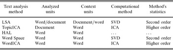
In this paper, we will consider two computational methods, singular value decomposition (SVD) and ICA, both applicable to the analysis of word contexts. Specifically, we analyze words and utilize the co-occurrences of the analyzed words with contexts units, namely other words. Table 1 provides a general comparison of related text analysis methods that utilize SVD, ICA and contexts.
The relationship between LSA, TopicICA, HAL, word space, and WordICA in terms of analyzed units, data, and the computational method

The main difference between the LSA and proposed WordICA approach is that LSA uses SVD for the statistical analysis, whereas WordICA uses the ICA method. Moreover, LSA is often used to analyze and represent documents whereas WordICA is used to do the same for words. However, both the ICA and SVD analysis can be conducted to representations at the level of documents, paragraphs, sentences or individual words. Schütze (Reference Schütze1992) has developed the Word Space method that utilizes both word-word matrices and SVD for representing word meaning and senses. Lund, Burgess and Audet (Reference Lund, Burgess and Audet1996) have developed the Hyperspace Analogue to Language (HAL) model, which is also based on a word-word matrix, but does not apply any dimension reduction or factorization techniques. Kolenda, Hansen and Sigurdsson (Reference Kolenda, Hansen and Sigurdsson2000) has applied ICA to topic analysis (labeled ‘TopicICA’ in Table 1).
1.2 Motivation for using independent component analysis
In this paper, we show that ICA applied on word context data gives distinct features that reflect linguistic categories. Hyvärinen, Karhunen and Oja (Reference Hyvärinen, Karhunen and Oja2001) give a thorough review of ICA. The WordICA analysis produces features or categories that are both explicitly computed and can easily be interpreted by humans. This result can be obtained without any human supervision or tagged corpora that would have some predetermined morphological, syntactic or semantic information. The results include both an emergence of clear distinctive features and a distributed representation. This is based on the fact that a word may belong to several features simultaneously in a graded manner. We wish that our model provides simultaneously in a graded manner. We propose that our model could provide additional understanding on potential cognitive mechanisms in natural language learning and understanding. Our approach suggests that much of the linguistic knowledge is emergent in nature and based on specific learning mechanisms.
Our approach is in line with the paradigm that is increasingly common within the area of cognitive linguistics. For instance, Croft and Cruse (Reference Croft and Cruse2004) outline three major hypotheses in the cognitive linguistic approach to language: (1) language is not an autonomous cognitive faculty, (2) grammar is conceptualization, and (3) knowledge of language emerges from language use. These three hypotheses represent a response to the earlier dominant approaches to syntax and semantics, i.e. generative grammar (Chomsky Reference Chomsky1975) and truth-conditional logical semantics (Tarski Reference Tarski, Bach and Harms1983; Davidson Reference Davidson2001). The first principle is opposed to the generative grammar's hypothesis that language is an autonomous and innate cognitive faculty or module, separated from nonlinguistic cognitive abilities (Croft and Cruse Reference Croft and Cruse2004). By the second principle, cognitive linguists refer to the idea that representation of linguistic structures, e.g., syntax, is also basically conceptual. From our point of view, this means that the basis of syntactic representations is subject to neurally based knowledge formation processes rather than given in some abstract way or genetically inherited. The third major principle states the idea that knowledge of language emerges from language use, i.e. categories and structures in semantics, syntax, morphology and phonology are built up from our cognition of specific utterances on specific occasions of use (Croft and Cruse Reference Croft and Cruse2004). We relate to this principle in a straightforward manner: the WordICA method facilitates emergence of features or categories by analyzing the use of words in their contexts. In the reported work, we focus on deriving the features from textual context but there is no principled limitation in using the approach in multimodal contexts (for a related approach, see Yu, Ballard and Asli Reference Yu, Ballard and Asli2003; Hansen, Ahrendt and Larsen Reference Hansen, Ahrendt and Larsen2005.)
In general linguistics, it is commonplace to specify a number of features that the words may have. This specification is based on the intellectual efforts by linguists who look for regularities in languages. For instance, linguistic features or so-called tags applied in the widely used Brown corpus (Francis and Kucera Reference Francis and Kucera1964) include predefined categories such as ‘preposition,’ ‘adjective,’ ‘superlative form of adjective,’ ‘noun,’ ‘noun in plural,’ ‘proper noun in plural,’ etc. The number of tags used in the Brown corpus is 82, including tags for POS categories, function words, certain individual words, punctuation marks of syntactic importance and inflectional morphemes. A central question for our work is whether we can learn similar features from a corpus automatically, and what the fit between the human-specified features and the automatically generated features would be. If one is able to obtain automatically a consistent and linguistically well-motivated set of features, it could facilitate, for instance, automatic generation of useful lexical resources for language technology applications such as natural language interfaces and machine translation. In machine translation, the automatically extracted POS-like features can be used at least in alignment and evaluation, as discussed in the previous section. Moreover, this kind of result would further support the major hypotheses or principles of cognitive linguistics listed above.
Next, we consider the use of ICA in the extraction of linguistic features for words in their contexts. ICA learns features in an unsupervised manner. Several such features can be present in a word, and ICA gives the explicit values of each feature for each word. We expect the features to coincide with known linguistic categories: for instance, we expect ICA to be able to find a feature that is shared by words such as ‘must,’ ‘can’ and ‘may.’ In earlier studies, ICA has been used for document level analysis of texts (see, e.g., Kolenda et al. Reference Kolenda, Hansen and Sigurdsson2000; Bingham, Kabán and Girolami Reference Bingham, Kuusisto and Lagus2002; Bingham, Kuusisto and Lagus Reference Bingham, Kuusisto and Lagus2002).
We first give a brief outline of SVD as well as the theory of ICA and other basic concepts.
1.3 Singular value decomposition and principal component analysis
Singular value decomposition is a method for matrix factorization, and it is an integral part of the LSA method, presented later in the paper. Moreover, SVD is one alternative as a typical preprocessing step for dimension reduction and whitening before an ICA analysis.
Suppose X is an m-by-n matrix (m < n). There exists a factorization of the form

where U is an m-by-m orthogonal matrix, the matrix D is an m-by-m diagonal matrix with nonnegative real numbers on the diagonal, and VT denotes the transpose of V, an n-by-m orthogonal matrix. This factorization is called the singular-value decomposition of X.
The SVD method is closely related to the principal component analysis (PCA) method that is widely used in statistical data analysis. The PCA method transforms a number of possibly correlated variables into a smaller number of uncorrelated variables called principal components. The PCA method is typically used as a preprocessing step for the ICA analysis to reduce the dimensionality of the original data, to uncorrelate the data variables, and to normalize the variances of the variables. As a textbook account on SVD and PCA one can use, e.g., Haykin (Reference Haykin1999).
1.4 Basic theory of independent component analysis
In the classic version of the ICA model (Jutten and Hérault Reference Jutten and Hérault1991; Comon Reference Comon1994; Hyvärinen et al. Reference Hyvärinen, Karhunen and Oja2001), each observed random variable is represented as a weighted sum of independent random variables. An example of an observed random variable in our case is the frequency of some word in a particular context. The independent random variables refer to the underlying variables.
We can illustrate some of the intuitions behind the ICA method through a practical example from another domain. For instance, the cocktail party problem is a classical blind signal separation task where heard sound signals are studied as the observed random variables. These are assumed to originate from a number of separate sources, in this case, the discussants in a cocktail party who are speaking at the same time. The heard signals are mixtures of the speech signals with different proportions depending on the relative distance of a listener to each sound source. The task is to separate the original speech signals from the observed mixtures.
The weights in the sum (which can be negative as well as positive) can be collected in a matrix, called the mixing matrix. The weights are assumed to be different for each observed variable, so that the mixing matrix can be inverted, and the values of the independent components can be computed as some linear functions of the observed variables.
Mathematically, the classic version of the ICA model can be expressed as

where x = (x 1, x 2, . . ., x C)T) is the vector of observed random variables, the vector of the independent latent variables is denoted by s = (s 1, s 2, . . ., s D)T) (the ‘independent components’), and A is an unknown constant matrix, called the mixing matrix. If we denote the columns of matrix A by ai the model can be written as

ICA finds the decomposition of (2) in an unsupervised manner. In other words, the method observes the mixtures of signals, x, and estimates both the mixing weights, A, and the original signals, s. This decomposition process does not require any samples of the original signals.
In the cocktail party problem, the goal of ICA is to learn the decomposition of the signals in an unsupervised manner, which means that we only observe the mixed signals and have no information about the mixing coefficients, i.e., the mixing matrix or the contents of the original signals.
ICA can be seen as an extension to PCA and factor analysis, which underlie LSA. However, ICA is a more powerful technique capable of making underlying factors explicit when the classic methods would not be able to do that. More precisely, ICA is more powerful than PCA if the underlying components are non-Gaussian. In fact, it can be shown that ICA is then capable to identify the original independent components (Comon Reference Comon1994), while PCA is not. From a practical point of view, the main difference of the two methods is that while PCA finds projections which have maximum variance, ICA finds projections which are maximally non-Gaussian.
While PCA is clearly inferior to ICA in terms of identifying the underlying factors, it is useful as a preprocessing technique because it can reduce the dimension of the data with minimum mean-squares error, by just taking the subspace of the first principal components. In contrast, the purpose of ICA is not dimension reduction, and it is not straightforward to reduce dimension with ICA.
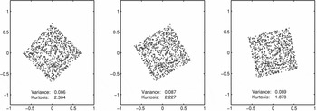
The classic methods of PCA and factor analysis are based on second-order moments (variance) whereas ICA is based on higher-order moments (e.g., kurtosis, see Hyvärinen et al. Reference Hyvärinen, Karhunen and Oja2001). This difference is summarized in Table 1 and the effect of this difference is illustrated in Figure 1.
Illustration on the effect of rotation on variance and kurtosis. The variance does not change due to the rotation but only slightly because of a limited set of samples. Kurtosis depends on the rotation and thus provides information beyond what the PCA and factor analysis can find. Here the variance and kurtosis are measured along the x-axis.

The starting point for ICA is the simple assumption that the components s i are statistically independent. Two random variables, y 1 and y 2, are independent if information on the value of y 1 does not give any information on the value of y 2, and vice versa. This does not need to hold for the observed variables x i. In case of two variables, the independence holds if and only if p(y 1, y 2) = p(y 1)p(y 2). This definition extends to any number of random variables. For instance in the case of the cocktail party problem, different original sources are typically approximately independent.
There are three properties of ICA that should be taken into account when considering the results of the analysis. First, one cannot determine the variances of the independent components s i. The reason is that, both s and A being unknown, any scalar multiplier in one of the sources s i could always be cancelled by dividing the corresponding column ai of A by the same scalar. As a normalization step, one can assume that each component has a unit variance, Var{s i} = E{s i2} = 1, with zero-mean components, E{s i} = 0. The ambiguity of the sign still remains: each component can be multiplied by −1 without affecting the model.
The second property to be remembered is that the order of the components cannot be determined. While both s and A are unknown, one can freely change the order of the terms in (3) and call any of the components the first one.
The third important property of ICA is that the independent components must be non-Gaussian for ICA to be possible (Hyvärinen et al. Reference Hyvärinen, Karhunen and Oja2001). Then, the mixing matrix can be estimated up to the indeterminacies of order and sign discussed above. This stands in stark contrast to such techniques as PCA and factor analysis, which are only able to estimate the mixing matrix up to a rotation. This would be quite insufficient for our purposes, as we wish to find components that would be cognitively interesting by themselves, instead of a latent set of components. Assuming that the components are independent as well as non-Gaussian, the rotation will separate the interesting components from the mixtures.
Independent component analysis is computed in a stochastic manner and the time complexity cannot be directly stated. However, the convergence of the Fast-ICA algorithm (Hyvärinen Reference Hyvärinen1999) is cubic, which makes it feasible to use with real applications. Compared to second-order methods such as SVD or PCA, ICA is always more complex, as it typically utilizes those in preprocessing. An empirical time complexity evaluation for PCA and ICA is presented in Appendix B.
1.5 Analysis of words in contexts
Contextual information has widely been used in statistical analysis of natural language corpora (see Church and Hanks Reference Church and Hanks1990; Schüetze Reference Schütze1992; Manning and Schütze Reference Manning and Schütze1999; Sahlgren Reference Sahlgren2006). Managing computerized form of written language rests on processing of discrete symbols. How can a symbolic input such as a word be given to a numeric algorithm? Similarity in the appearance of the words does not usually correlate with the semantics they refer to. As a simple example one may consider the words ‘window,’ ‘glass,’ and ‘widow.’ The words ‘window’ and ‘widow’ are phonetically close to each other, whereas the semantic relatedness of the words ‘window’ and ‘glass’ is not reflected by any simple metric. For the reasoning above, we do not take into account the phonetic or orthographic form of words, but have a distributional representation instead.
One useful distributional numerical representation can be obtained by taking the sentential context in which the words occur into account. First, we represent each word by a vector, and then code each context as a function of vectors representing the words in that context. A context can be defined, for instance, as a sequence of consecutive words in text. The basic idea is that the distributional similarity of words is analyzed. In the simplest case, the dimension is equal to the number of different word types, each word is represented by a vector with one element equal to one and others equal to zero. Then the context vector simply gives the frequency of each word in the context. In information retrieval, this is called the bag-of-words model, in which the text is represented as an unordered collection of words, disregarding grammar or word order. The bag-of-words model provides a straightforward way to represent documents and queries in a shared vector space (Salton, Wong and Yang Reference Salton, Wong and Yang1975). The bag-of-words model can be used to compare the similarity of contexts, i.e. similar contexts have similar vectorial representations. For computational reasons, the dimension may be reduced by different methods. A more compact representation can also be said to generalize similarities in the space of the words. A popular dimension reduction technique for text is SVD, which is explained in more detail in Section 1.3.
1.6 Non-Gaussianity and independence in text data
The assumption of non-Gaussianity for the components in ICA is necessary because the Gaussian distribution is, in some sense, too simple. Specifically, all the information about a multivariate Gaussian distribution is contained in the covariance matrix. However, the covariance matrix does not contain enough parameters to constrain the whole matrix A, and thus the problem of estimating A for Gaussian data is ill-posed (Comon Reference Comon1994).
Another point of view is that uncorrelated (jointly) Gaussian variables are necessarily independent. Thus, independence is easy to obtain with Gaussian variables since transforming multivariate data into uncorrelated linear components is a straightforward procedure, for instance, with PCA or SVD. For a model with non-Gaussian components, however, independence is a much stronger property, and allows the ICA model to be estimated based on the non-Gaussian structure of the data.
Natural signals based on sensory data are typically non-Gaussian (see, e.g., for image data, Hyvärinen, Hurri and Hoyer, Reference Hyvärinen, Hurri and Hoyer2009). Text data is not ‘natural’ in the same sense, since it is based on an encoding process. However, word contexts seem to be non-Gaussian because of the sparseness of the data. A sparse distribution is one in which there is a large probability mass for values close to zero, but also heavy tails (cf. Zipf's law). This is shown as values with a large proportion of small values and zeros and only a few large values, which is intuitively related to ‘on/off’ data with mostly ‘off’ values. Thus, ICA tries to represent each word with only a few clearly active components, which is related to sparse coding (Hyvärinen et al. Reference Hyvärinen, Hurri and Hoyer2009). The justification for using ICA for word contexts could thus be that human cognition encodes language in a way similar to such sensory-level sparse coding. We are not trying to claim, in general, that the brain ‘does ICA,’ but that the underlying principles of efficient neural coding may be similar.
1.7 Latent semantic analysis
Latent semantic analysis is a technique for analyzing relationships between documents and terms. LSA was originally introduced as a new approach to automatic indexing and retrieval (Deerwester et al. Reference Deerwester, Dumais, Landauer, Furnas and Harshman1990), and is often called latent semantic indexing (LSI) in that field. The technique behind LSA is SVD (1).
In LSA, SVD is used to create a latent semantic space. First, a document-term matrix X is generated. Every term (for instance, a word) is represented by a column in matrix X, and every document is represented by a row. An individual entry in X, x dn, represents the frequency of the term n in document d. The raw frequencies are typically processed, for instance, with log-entropy or tf-idf weighting. Next, SVD is used to decompose matrix X into three separate matrices using (1). The first matrix is a document by concept matrix U. The second matrix is a concept by concept matrix D. The third matrix is a concept by term matrix VT. The context for each word in basic LSA is the whole document. A notable difference is that in our ICA and SVD experiments (explained later in this paper), we used a local context, i.e. the immediately preceding and following words, which will bring out more syntactic information. This contrasts with LSA that uses document-term matrices and finds topical information. This difference in the effect of using short versus long contexts is highlighted by comparing the results of earlier experiments using different methods (see, e.g., Bingham et al. Reference Bingham, Kabán and Girolami2001, Reference Bingham, Kuusisto and Lagus2002; Levy, Bullinaria and Patel Reference Levy, Bullinaria and Patel1998; Sahlgren Reference Sahlgren2006) and the results reported later in this paper. Intuitively, the difference stems from the fact that the use of long contexts with the bag-of-words model hides practically all grammatical information.
Landauer and Dumais (Reference Landauer and Dumais1997) describe LSA in terms of learning and cognitive science. The claim is that LSA acquired knowledge about the full vocabulary of English at a rate comparable to school-children. The development of LSA has also been justified through practical applications by Furnas et al. (Reference Furnas, Landauer, Gomez and Dumais1987), such as cross-language retrieval (Dumais et al. Reference Dumais, Letsche, Littman and Landauer1997), word sense disambiguation (Niu et al. Reference Niu, Li, Srihari, Li and Crist2004), text summarization (Steinberger et al. Reference Steinberger, Kabadjov, Poesio and Sanchez-Graillet2005), text segmentation (Choi, Wiemer-Hastings and Moore Reference Choi, Wiemer-Hastings and Moore2001), and measurement of textual coherence (Foltz, Kintsch and Landauer Reference Foltz, Kintsch and Landauer1998).
One important problem with LSA, however, is that the latent concept space is difficult to understand by humans. In this paper, we present a method to overcome this limitation. Earlier related attempts include Finch and Schütze (Reference Finch, Chater, Aleksander and Taylor1992), Schütze (Reference Schütze1995), and Clark (Reference Clark2000). Schütze (Reference Schütze1995) presented a method for tag induction in which the results of SVD were clustered into 200 distinct classes and further compared with approximately the same number of POS tags used in the Brown corpus (Francis and Kucera Reference Francis and Kucera1964). His method produces one POS tag per word from a predefined tag set (which very much resembles the approach taken in Ritter and Kohonen Reference Ritter and Kohonen1989; Honkela Pulkki and Kohonen Reference Honkela, Pulkki and Kohonen1995 using the self-organizing map as the clustering algorithm). In contrast, our WordICA method automatically creates a feature representation of the words without human supervision. Our method can be contrasted with another unsupervised approach by Clark (Reference Clark2000), in which contexts are clustered to create groups of words that have been used in similar manner. Clark's methods handle ambiguity and low frequency words well.
The WordICA method provides multiple emergent features per word. Rather than clusters, these features are morphological, syntactic and semantic markers. Many of these features seem to coincide with the traditional tags used, for instance, in the Brown corpus. We present the comparison in Section 3. Moreover, the values of the word features are continuous.
2 Data and methods
Here we describe the data sets and methods used in the experiments. We explain how the contextual information was collected and represented for the two experiments. The first one is a small scale experiment with manual detailed analysis that shows that the results follow our initial assumptions. More specifically, the results indicate that the emergent representations are sparse and the features, in a qualitative analysis, correspond to linguistically meaningful categories. The second experiment uses a larger data set and is used to quantitatively evaluate whether the method produces features that reflect categories created by human linguistic analysis.
2.1 Data and context matrix formation
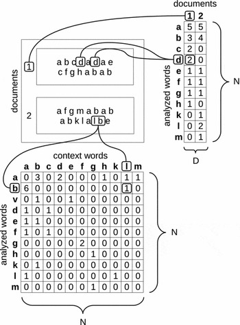
We first describe the method for creating context matrices in its general form. Thereafter, we present the data and the specific preprocessing parameters used in our experiments. As the first step of the WordICA method, the most frequent N words, or some other subset of N words, from the corpus are selected as the vocabulary to be analyzed. For the context words, M of the most frequent words are selected. Each context is defined by one of the context words and a location related to the analyzed word. This is illustrated in Figure 2. A location can be, for instance, the immediately preceding word or any of the two preceding words or two following words.
Illustration on how text documents are transformed into word-document matrices (on the right hand side) and word-word matrices (below). In this particular word-context matrix, it has been indicated how many times a context word (e.g., ‘l’) appears immediately to the left from each word (e.g., ‘b’). The word-document matrix simply indicates the number of occurrences of each word in each document.

The number of different contexts depends on the selected context words and the locations. An M-by-N word-word matrix X is formed in which x cn denotes the number of occurrences of the n:th analyzed word with the c:th context word. The data matrix X is preprocessed by taking the logarithm of the frequencies increased by one. Taking the logarithm dampens the differences in the word frequencies. This makes the computational methods model the most frequent words less and enables finding more interesting phenomenon from the data. The co-occurrence frequencies are smoothed by adding one to all frequencies (originating from Laplace's rule of succession). This makes the prior assumption that all possible co-occurrences can happen with equal probability. Furthermore, this makes the argument for the logarithm positive, without changing the sparsity of the data matrix as logarithm of one is zero.
This kind of gathering of contextual information and representation of the produced context-word matrix was conducted separately for the two data sets explained next with detailed parameter values.
2.1.1 Data set 1: Connectionists e-mails
The data used in the small scale experiment consists of a collection of e-mails sent to the Connectionists mailing list. The texts were concatenated into one file. Punctuation marks were removed and all uppercase letters were replaced by the corresponding lowercase letters. The resulting Connectionists E-mail corpus consists of 4,921,934 tokens (words in the running text) and 117,283 types (different unique words).
The most frequent nouns, verbs, articles, conjunctions, and pronouns were included in the analysis. In addition, some additional words were added to provide more complete view on selected categories (e.g., ‘did’ to complement the verb ‘do’ that belongs to the most frequent words). The list of words N = 100 is shown in Appendix A. The contextual information was calculated using the M = 2,000 most frequent types, where the context word immediately followed the analyzed word. No stopword list was in use. This provided a 2,000 × 100 matrix X. The data is available at http://www.cis.hut.fi/research/cog/data/wordica/ including the data matrix and the list of words used in the analysis.
In this experiment, we used a word-context matrix that is a transpose of the context-word matrix X. Both data matrices X and XT can be given to ICA, however, the independence assumptions (i.i.d. for the data, independence of components) are targeted differently given the orientation of the data matrix. A similar idea has been applied with successful results to functional brain imaging data, where different orientations produce temporal ICA and spatial ICA for components that span either time or space, respectively (McKeown et al. Reference McKeown, Makeig, Brown, Jung, Kindermann, Bell, Iragui and Sejnowski1998). However, the difference is not significant for the results in the present application.
2.1.2 Data set 2: Gutenberg e-books
We used the same English corpus of a collection of different texts from Project Gutenberg as in Honkela, Hyvärinen and Väyrynen (Reference Honkela, Hyvärinen and Väyrynen2005) and in Väyrynen, Honkela and Hyvärinen (Reference Väyrynen, Honkela and Hyvärinen2004). The preprocessing was conducted in a simple manner. In summary, most of the nonalphanumeric characters were removed and the remaining characters were converted to lowercase. The resulting corpus consisted of 21,951,835 tokens with 188,386 types.
For the analysis, only words that were also present in the Brown corpus (see Section 2.1.3) were considered. This ensured that there was at least one tag for each analyzed word. The N = 10,000 most frequent words in the Gutenberg corpus from those were selected as the vocabulary to be analyzed. Contextual information was calculated based on the most frequent thousand words in the Gutenberg corpus, without the limitation to words in the tagged Brown corpus. Contexts were calculated separately for the context words immediately following and preceding the analyzed words (M = 2 × 1,000 = 2,000). This resulted in a 2,000 × 10,000 data matrix X.
2.1.3 Tagged brown corpus
For evaluation purposes only, we also used the POS tagged Brown corpus (Francis and Kucera Reference Francis and Kucera1964). The word category information was extracted from a subset of the corpus that had a single word category tag t k assigned to each word token. We collected the possible tags for each word type.
The word categories collected from the tagged Brown corpus were encoded as column vectors ck of length N. The element c kn was set to one if the n:th analyzed word occurred together with the k:th tag, and zero otherwise. Each analyzed word belonged to at least one word category because all analyzed words were present in the Brown corpus as well. Word categories without any words in the analyzed vocabulary were removed, which left K = 58 word categories and binary-valued word category vectors ck, k = 1,. . ., K.
2.2 Feature extraction
Our goal was to extract a number of features fi from the context-word matrix X. Next, we show how ICA and SVD are used to extract features from data, and how SVD can be seen as a preprocessing step to ICA.
Singular value decomposition (see Section 1.3)

explains the data X in terms of left singular vectors in U, singular values in D, and right singular vectors in V. The singular vectors are orthogonal

and D is a diagonal matrix. The vectors in U and V are usually sorted according to the values of the corresponding singular values in the diagonal of D. Dimension reduction can be done by selecting the largest singular values and the corresponding vectors, i.e. setting the smallest singular values to zero. In our experiments, Matlab command svds was used to extract a pre-specified number of the largest singular values and vectors. The reduced matrix VT of right singular vectors gives the SVD feature representation for words.
The linear generative model

of ICA (see Section 1.4) in matrix form explains the rows of the data matrix X in terms of a mixing matrix A and independent components S by assuming the independence of the rows of S. We used the FastICA Matlab package (Hurri et al. Reference Hurri, Gävert, Särelä and Hyvärinen2002) to extract a prespecified number of features. The independent components in matrix S gives the ICA feature representation for words.
In the following, we consider only zero mean data (rows of X).If the data is not zero mean, the mean can simply be removed before applying SVD and ICA. After the computation, the transformed mean can be returned to the linear models.
In practice, we first perform PCA to decorrelate the data rows and set variances to one, i.e. the data correlation matrix is a unit matrix. The process is called whitening. The dimensionality of the data is also reduced with PCA to the number of extracted features. Any other whitening and dimension reduction method could be used, for instance, the applied method is equivalent to using SVD and reducing the data matrix by only retaining the columns of U and V which correspond to the largest singular values. The preliminary whitening that is typically performed in ICA can be achieved by taking just the corresponding columns of V as the rows of the whitened data. The ICA problem now reduces to finding a square whitened mixing matrix B = UDA which follows the ICA model VT = BS for whitened data. For whitened data the mixing matrix B is a rotation matrix. Based on the assumption of independence, ICA is particularly useful for extracting the underlying structure in the data. More specifically, ICA rotates the original SVD feature space in such a way that each of the features tends to become a meaningful representation of some linguistically motivated phenomenon. The feature space thus transforms from a latent feature space into a space where each of the features carry meaning, for instance, syntactic or semantic linguistic information in our analysis of words in contexts. The nature of the emergent features of course depends on the formulation of the data matrix X. For instance, the result is dependent on how the contexts are specified and which words are included in the analysis.
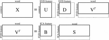
The two feature extraction methods (SVD and ICA) are illustrated in Figure 3. The matrices ST and V have the feature vectors fi as columns. We will use the notation fi for the feature vectors regardless of the extraction method. The feature vectors fi were scaled to unit variance as a postprocessing step after the feature extraction in order to facilitate the comparison between SVD and ICA results. The feature vectors can be understood to be encoded similarly to the rows of the data matrix X, where the value of the n:th element says something about the n:th word.
Illustration on how SVD ((4), top illustration) and ICA ((6), bottom illustration) are related in the process of analyzing zero-mean context data for words. The dotted lines represent the whole feature spaces and the full lines represent data after dimension reduction. Here ICA operates on whitened data VT and the whitened mixing matrix B is a square rotation matrix. The extracted features for SVD and ICA are the rows of VT and S, respectively.

In the experiments, we used the standard maximum-likelihood estimation by setting the nonlinearity in FastICA (Hyvärinen Reference Hyvärinen1999) to the tanh function, and using symmetric orthogonalization (Hyvärinen et al. Reference Hyvärinen, Karhunen and Oja2001). The dimensionality of the data was reduced by PCA (this is implemented as part of the software). Reduction of the dimensionality is often used to reduce noise and overlearning (Hyvärinen et al. Reference Hyvärinen, Karhunen and Oja2001).
2.3 Comparison method
The comparison of the emergent features and manually defined tags is not straightforward. The basic reason for not using, for example, standard information retrieval evaluation measures such as precision and recall, is the fact that the analysis results are continuous, not discrete. More specifically, we do not discretize the extracted features by, for instance, clustering, which would again deconstruct the result obtained by the analysis. In other words, we do not want to divide the feature space into disjoint areas, because the study of the properties of individual features is an essential task. Another important reason is that the automatically extracted features do not need to have a one-to-one mapping with the manually defined tags. Therefore, we have developed a comparison method for this specific need, strongly suggesting that this approach is necessary because of the unusual comparison setting.
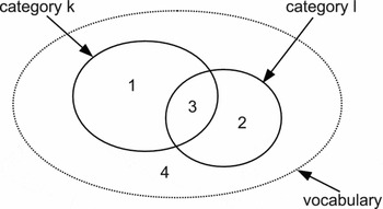
Next, we describe in detail the method we used to compare the results of feature extraction methods (SVD and ICA) with manually constructed tags. Considering two word categories k and l and the corresponding word category vectors ck and cl, the words w n in the vocabulary can be divided into four types:
(1) words belonging to category k and not to l,
(2) words belonging to category l and not to k,
(3) words belonging to both categories k and l, and
(4) words belonging neither to category k nor to l,
where each word w n belongs to exactly one of these types. This is illustrated in Figure 4. Considering only two feature for each word, we can examine how well those features with continuous values correspond to the crisp categories.
Illustration of the four types of words when considering categories k and l. The space of all words in the vocabulary inside the dotted ellipse is divided into four disjoint areas. Each word w n in the vocabulary belongs to exactly one of these areas.

A two-dimensional subspace of two feature vectors fi and fj can be visualized as a scatterplot, where the points (x n, y n) = (f i(n), f j(n)), n = 1,. . ., N are the words w n in the vocabulary. The separation capability of the individual features can be analyzed by studying the locations of the four disjoint types of words in the plane. What we want is to see type 1 and 2 words (see above) in their own axis away from the origin, type 3 words away from the origin, and type 4 words in the origin. A novel separation measure (Väyrynen and Honkela Reference Väyrynen and Honkela2005) rewards or penalizes words depending on the position on the plane and the type of the word. The words in type 3 represent ambiguity in language and are considered separately from the words in the first two types.
Next, we will describe the separation measure we used in comparing the learned features (Väyrynen and Honkela Reference Väyrynen and Honkela2005). The measure works in three steps. First we calculate the amount of separation that two features create for two word categories. Secondly, we choose the best feature pair separating two categories. Finally, we consider the mean separation capability of a set of features for a set of categories. This average measures how well the emergent features are organized with respect to the given categories.
The separation capability of two features i and j and two word categories k and l is calculated as the mean of the rewards and penalties over all N words as

with the rewards split into four parts corresponding to the four disjoint types:
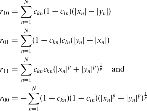
where distance from the origin is calculated using the p-norm distance metric. In our experiments, we had the Euclidean distance (p = 2). A positive value is given to a word located in a place that is beneficial to the separation of the word categories and acts as a reward, whereas a negative value is considered a penalty. The larger the value of sep(k, l, i, j), the better the separation is according to the measure.
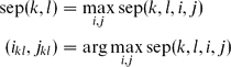
With the method, we can see if a word category is always best separated by the same feature when compared against other word categories. If the learned features are mixtures of the word categories, the best separating feature might differ when tested against different word categories. The best feature pair (i kl, j kl) for the word category pair (k, l) is selected as the pair giving the highest value with the separation measure
The separation capability of a feature set is measured as the mean of the best separation over all word category pairs
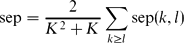
where K is the number of word categories.
It is important to compare the capability of single features or feature pairs to separate categories because this measures how well the obtained features correspond to the categories. In fact, when all features are used, the separation capabilities of ICA and SVD are comparable because the total information present is the same, as discussed in detail by Vicente, Hoyer and Hyvärinen (Reference Vicente, Hoyer and Hyvärinen2007). The reason for not using standard information retrieval evaluation measures such as precision and recall is the fact that the analysis results are continuous, not discrete. Another reason is that we do not expect and require the results to have a one-to-one mapping between the manually defined tags and ICA-based emergent features.
3 Results
We now turn to the results and evaluation of the extracted features from the two experiments. The first experiment used a rather small text corpus of Connectionists e-mails, introduced in Section 2.1.1, with 100 analyzed words, 2,000 different contexts and 10 extracted features. The resulting features were analyzed in detail by hand. The study showed that our initial assumptions of the nature of the emergent features were correct. In particular, the features correspond reasonably well with linguistically motivated categories and they also form a sparse representation of the data.
The second experiment used a larger corpus of Gutenberg e-books, introduced in Section 2.1.2, with 10,000 analyzed words, 2,000 different contexts and 100 extracted features. A manual analysis is not feasible due to the large number of words and features. The match between the extracted features and syntactic tags for words extracted from the tagged Brown corpus was computed for features extracted with both SVD and ICA using the separation measure introduced in Section 2.3.
3.1 Experiment with connectionists list
The results of the ICA analysis corresponded in most cases very well or at least reasonably well with our preliminary intuitions. The system was able to create automatically distributed representations as a meaningful collection of emergent linguistic features; each independent component was one such feature.
Next, we will show several examples of the analysis results. In considering the feature distributions, it is good to keep in mind that the sign of the features is arbitrary. Again, as was mentioned earlier, this is because of the ambiguity of the sign: the components can be multiplied by −1 without affecting the model (see Section 1.4).
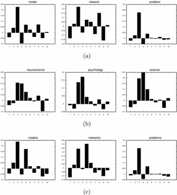
Figure 5(a) shows how the third component is strong in the case of nouns in singular form. A similar pattern was present in all the nouns with three exceptional cases with an additional strong fourth component indicated in Figure 5(b). The reason appears to be that ‘psychology’, ‘neuroscience’, and ‘science’ share a semantic feature of being a science or a scientific discipline. This group of words provides a clear example of distributed representation where, in this case, two components are involved.
(a) ICA representation for ‘model,’ ‘network,’ and ‘problem.’ (b) ICA representation for ‘neuroscience,’ ‘psychology,’ and ‘science.’ (c) ICA representation for ‘models,’ ‘networks,’ and ‘problems.’

An interesting point of comparison for Figure 5(a) is the collection of plural forms of the same nouns in Figure 5(c). The third component is strong as with the singular nouns but now there is another strong component, the fifth.
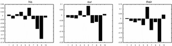
Figure 6 shows how all the possessive pronouns share the feature number nine.
ICA representation for ‘his’, ‘our,’ and ‘their.’

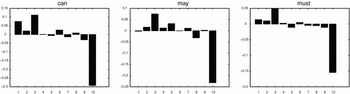
Modal verbs are represented clearly with component number ten as shown in Figure 7. Here, slightly disappointingly, the modal verbs are not directly linked with verbs in general through a shared component. This may be because of the distinct nature of the modal verbs. Moreover, one has to remember that in this analysis we used ten as the number of ICA features which sets a limit on the complexity of the feature encoding. We used this limit in order to demonstrate the powerfulness and usefulness of the method in a simple manner. A higher number of features can be used to obtain more detailed feature distinctions.
ICA representation for ‘can’, ‘may,’ and ‘must.’

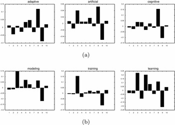
Figure 8(a) shows how the adjectives are related to each other through the shared feature number eight, and even number nine in the opposite direction. Quite interestingly, this component number nine is associated with ing-ending verbs (see Figure 8b) such as ‘modeling,’ ‘training,’ and ‘learning’ that can, naturally, serve in the position of an adjective or a noun (consider, for instance, ‘training set’ versus ‘network training’).
(a) ICA representation for ‘adaptive,’ ‘artificial,’ and ‘cognitive.’ (b) ICA representation for ‘modeling,’ ‘training,’ and ‘learning.’

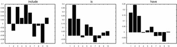
Finally, there are individual words, particularly some verbs, for which the result is not as clear as for other words. In Figure 9 it is shown how the verb ‘include’ and the copula ‘is’ have several features present in a distributed manner. The word ‘is’ clearly shares, however, the feature number two with the word ‘have.’ This slight anomaly particularly concerning ‘include’ may also be related to the fact that ten features were used for the hundred words. For a related reason, a collection of particles and similar frequent words were excluded from the analysis because many of them are rather unique in their use considering the contexts in which they appear. In other words, representatives of linguistics categories such as nouns and verbs share general characteristics in the patterns of their use, whereas each particle has a specific role profile which clearly differs from the use of other particles. This phenomenon was already discernable in the analysis of word contexts using the self-organizing map (Honkela et al. Reference Honkela, Pulkki and Kohonen1995).
ICA representation for ‘include’, ‘is,’ and ‘have.’

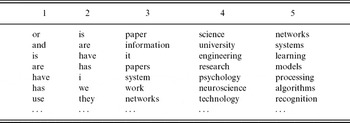
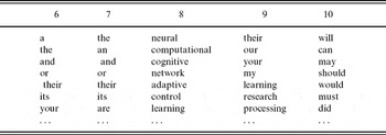
The categorical nature of each component can also be illustrated by listing the words that are strongest in each component (see Tables 2 and 3). The result shows some very clear components such as 3–5 which can be considered noun categories. These three components were already discussed earlier. Component number 8 is populated by adjectives, whereas number 10 contains modal verbs. Verbs ‘to be’ and ‘have’ are in their different forms in the component 2. We can also see a certain kind of component overloading in components 1 and 2. This is explained by the limited number of component in use. With a larger number of components, a more detailed representation of the linguistic phenomenon can be gained (Borschbach and Pyka Reference Borschbach and Pyka2007). In general, the issue of choosing an optimal number of components is an open question both for an ICA-based method as well as for an SVD-based method such as LSA.
The most representative words for the first five features, in the order of representativeness, top is highest

The most representative words for the last five features, in the order of representativeness, top is highest

The nouns ‘network’ and ‘control’ in component 8 in Figure 3 are often used in the corpus in noun phrases like ‘neural network society.’ In general, the area and style of the texts in the corpus are, of course, reflected in the analysis results.
3.2 Experiment with Gutenberg corpus
Next, we show several examples of the analysis results based on the Gutenberg corpus. As was mentioned earlier, because of the ambiguity of the sign the components can be multiplied by −1 without affecting the model.
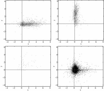
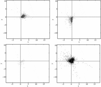
Figures 10 and 11 compare a single word category pair with the best found feature pair separating the word categories according to (7). The tag naming is adopted from the Brown corpus, with JJ for category ‘adjective’ and VB for category ‘verb, base: uninflected present, imperative or infinitive.’ In both figures, 60 features were extracted using SVD and ICA. The best found feature pair separating the two categories is more clearly aligned with the coordinate axis for the ICA-based features. With both methods, the shown features were consistently chosen to represent the JJ and VB categories when they were tested against all feature pairs.
The best ICA feature pair separating the JJ (adjective) and the VB (verb) categories with (7). The two upper diagrams show the distribution of the words belonging only to the category JJ (upper left) and VB (upper right). The lower left scatter plot shows the distribution of the words that belong to both categories. The lower right diagram consists of words from neither category. Some of the words on the right from the origin appear to have the characteristics of the listed adjectives, including adverbs and untagged adjectives.

The found best SVD feature pair separating the JJ (adjective) and the VB (verb) categories with (7). The scatter plots show the words in the four types plotted in the subspace created by the two features. The basic interpretation of the diagram is the same as for Figure 10. The result clearly indicates that the SVD analysis is unable to detect single features that would correspond to existing categories based on linguistic intuition and analysis.

Figure 12 shows the average separation over the feature set with (8) for the ICA-based and the SVD-based features as a function of the number of extracted features. Compared to SVD, the FastICA algorithm is not guaranteed to give exactly the same features for each computation because it starts from a random starting point. This variation was taken into account by running the ICA algorithm five times and calculating the mean and standard deviation of the separation measure for each extracted feature set. The ICA-based features give clearly higher separation compared to SVD-based features. The separation capability increases with the number of extracted features, as would be expected.
Comparison between ICA (upper curve) and SVD (lower curve) as a function of the number of extracted features. The y-axis shows the separation calculated with (8), and higher values indicate better separation. For the ICA-based features the mean and one standard deviation of five different runs is shown.

4 Conclusions and discussion
We have shown how ICA can find explicit features that characterize words in an intuitively appealing manner, in comparison with, for instance, SVD as the underlying computational method for LSA. We have considered WordICA for the analysis of words as they appear in text corpora. ICA appears to enable a qualitatively new kind of result. It provides automatically a result that resembles the manual formalization, e.g., based on the classical case grammar Fillmore (Reference Fillmore, Bach and Harms1968) and other similar approaches that represent the linguistic roles of words. SVD provides comparable results lacking, however, the explicitness of the distinct emergent features.
The analysis results show how the ICA analysis is able to reveal underlying linguistic features solely based on the contextual information. The results include both the emergence of clear distinctive categories or features as well as a distributed representation based on the fact that a word may belong to several categories simultaneously.
An important question is why the ICA analysis is able to reveal meaningful features when SVD and related methods are not. The methodologically oriented answer is based on the fact that independent components are typically found by finding maximally non-Gaussian components. This often means learning a maximally sparse representation for the data. The reasoning is that human cognition encodes information in a very similar fashion. We do not claim in general that the brain does ICA, but that the underlying principles of efficient neural coding brings forth quite similar representations. Suggestive evidence exists supporting the claim that process-level similarity between brain and ICA-like processes can be found in, at least, the area of visual cognition (Hyvärinen et al. Reference Hyvärinen, Hurri and Hoyer2009). The results shown in this paper suggest that this could be true also in the case of linguistic processing.
The distributed representation can be used as a low-dimensional encoding for words in various applications. The limited number of dimensions brings computational efficiency whereas the meaningful interpretation of each component provides a basis for intelligent processing. In Section 3.2, we showed that there is a clear relationship between emergent features and syntactic features.
Unsupervised learning can provide better generalization capability than supervised methods that are restricted to the annotated corpus, even if more unannotated material is readily available. Also, a linguistically motivated structure or typology may not be the perfect solution to each application. A good example of this is given in (Hirsimäki et al. Reference Hirsimäki, Creutz, Siivola, Kurimo, Virpioja and Pylkkönen2006), where unsupervised morphological analysis of words gave better results than traditional morphological analysis in the application of unlimited vocabulary automatic speech recognition. The applied method (Creutz and Lagus Reference Creutz and Lagus2007) segments words into statistical morphemes based on a corpus of text only, i.e. it does not depend on any given set of morphemes, and is able to segment previously unseen words. How these out-of-vocabulary words are dealt with is often crucial to the performance of a natural language engineering applications such as speech recognition (Bazzi and Glass Reference Bazzi and Glass2000).
In the future, we will also evaluate the usefulness of the WordICA method in various applications including natural language generation and machine translation. For machine translation, it seems that the WordICA method can be expanded into the analysis of parallel corpora. Preliminary experiments show that related words in different languages appear close to each other in the component space. This might even make it possible to find translations for words and phrases between languages (Väyrynen and Lindh-Knuutila Reference Väyrynen and Lindh-Knuutila2006). It would also be interesting to adapt the topical analysis models of latent Dirichlet allocation (Blei, Ng and Jordan Reference Blei, Ng and Jordan2003) and discrete PCA (Buntine and Jakulin Reference Buntine and Jakulin2004) to word analysis and compare the results to ICA. Moreover, it is also worth while to study how encoding the relative position of terms in a sliding window influences the results of the analysis (Jones and Mewhort Reference Jones and Mewhort2007; Sahlgren, Holst and Kanerva Reference Sahlgren, Holst and Kanerva2008).
In summary, we are optimistic that the WordICA method will be relevant in language technology applications such as information retrieval and machine translation, as well as in cognitive linguistics as a provider of additional understanding on potential cognitive mechanisms in natural language learning and understanding.
Acknowledgments
This work was supported by the Academy of Finland through the Adaptive Informatics Research Centre that is a part of the Finnish Centre of Excellence Programme and HeCSE, Helsinki Graduate School in Computer Science and Engineering. We warmly thank the anonymous reviewers and the editors of the journal as well as our colleagues, in particular, Oskar Kohonen, Tiina Lindh-Knuutila, and Sami Virpioja, for their detailed and constructive comments on earlier versions of this paper.
Appendix A: Connectionists data
The list of the 100 words with their frequencies used in the Connectionists experiment is shown below. The full data is available at http://www.cis.hut.fi/research/cog/data/wordica/.

Appendix B: Time complexity evaluation
Running times for PCA and ICA as a function of the number of extracted features are presented in the following. All the experiments were run in Matlab. PCA was computed with the eigs command for the covariance matrix of the data. PCA timings include computing the covariance matrix, computing PCA, projecting the data to a reduced space, and whitening. ICA was computed with the FastICA Matlab package (Hurri et al. Reference Hurri, Gävert, Särelä and Hyvärinen2002) for the whitened data with reduced dimension, and thus does not include the time used for preprocessing. The ICA timings include computing the ICA rotation and projecting the rotated whitened data back to the original space. The command cputime was used to measure the used CPU time in seconds. Each experiment was run 100 times and the average timings are shown.
PCA was computed for several N-by-M cooccurrence matrices computed from the Gutenberg corpus. The most frequent words were selected as the words chosen for the four experiments with different matrix sizes: 100-by-500, 250-by-500, 100-by-2,000, and 250-by-2,000. PCA was used to whiten the data and reduce the dimension to the number of extracted features. PCA timings are shown in Figure 13. The output of PCA was selected as the input to ICA, which rotated the whitened data and projected the result back to the original space. ICA timings are shown in Figure 14.
PCA timings for an N-by-M matrix as the number of extracted features.

ICA timings for an N-by-M matrix, which has already been whitened and reduced to an F-by-M matrix with PCA, as the number of extracted features F.

Even though this experiment considers only small input matrices, some conclusions can be made. The timings for PCA are considerably lower than for ICA. More significantly, the PCA timings grow roughly linearly with the number of features, whereas the ICA timings grow more rapidly. The number of rows (N) has a greater effect for PCA, whereas the ICA timings are clearly dominated by the number of columns (M). This is because PCA is calculated for the covariance matrix with size N-by-N, whereas ICA uses the projected lower dimensional data that has the same number of rows as the number of extracted features, which is typically lower than the number of columns.