
1. Introduction
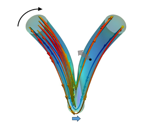
The complex interactions between different spatial and temporal scales of vortical flows are critically important to understanding the aerodynamic sound generated by turbulent flows (He, Jin & Yang Reference He, Jin and Yang2017). Vortex rings are vital candidates for the ‘elementary excitation’ of turbulent flows (Shariff & Leonard Reference Shariff and Leonard1992; Yao & Hussain Reference Yao and Hussain2022; Matsuzawa et al. Reference Matsuzawa, Mitchell, Perrard and Irvine2023). The investigation of vortex rings can date back to Helmholtz (Meleshko Reference Meleshko2010) and is still an active area of fundamental research. For example, recent work has examined the generation and evolution of vortex rings under different conditions (Limbourg & Nedić Reference Limbourg and Nedić2021; Wang & Feng Reference Wang and Feng2022), the writhing and twisting of vortex rings (Hattori et al. Reference Hattori, Blanco-Rodríguez and Le Dizès2019; Ortega-Chavez, Gan & Gaskell Reference Ortega-Chavez, Gan and Gaskell2023; Shen et al. Reference Shen, Yao, Hussain and Yang2023), impingement on walls (New et al. Reference New, Long, Zang and Shi2020; Chen et al. Reference Chen, Yoas, Jaworski and Krane2022; Ahmed & Erath Reference Ahmed and Erath2023), and the collision of vortex rings (Hernandez & Reyes Reference Hernandez and Reyes2017; McKeown et al. Reference McKeown, Ostilla-Mónico, Pumir, Brenner and Rubinstein2018; Hu & Peterson Reference Hu and Peterson2021; Mishra, Pumir & Ostilla-Mónico Reference Mishra, Pumir and Ostilla-Mónico2021; Nguyen Reference Nguyen2022). The interactions of vortex rings have been recognised as one of the few clean aeroacoustic scenarios because they isolate the end-effects of other configurations and help in identifying individual events as sound sources (Shariff & Leonard Reference Shariff and Leonard1992; Kambe Reference Kambe2010). The interactions of two vortex rings can be categorised into coaxial interactions and oblique interactions.
The aerodynamic sound generated by coaxial interactions of two vortex rings has been extensively investigated over the past few decades. Coaxial interactions include the leapfrogging, slip-through, mutual trapping and head-on collision of vortex rings (Borisov, Kilin & Mamaev Reference Borisov, Kilin and Mamaev2013). Möhring (Reference Möhring1978) proposed a vortex sound formula to compute aerodynamic sound generated by vortical flows at low Mach numbers and investigated the aerodynamic sound radiated from a pair of leapfrogging vortex rings. The results showed that the vorticity orthogonal to the observer vector contributes to the generation of sound. The two vortex rings are assumed to move as a pair of rectilinear spinning vortices by considering very thin rings, where the separation distance between the rings was much smaller than their diameters and much larger than their core diameters. Kambe & Minota (Reference Kambe and Minota1981) improved the interactions between vortex rings by using the Dyson thin core vortex ring model for inviscid flows. Their investigation on the leapfrogging of a vortex ring pair showed that the peak aerodynamic sound is generated at the instant when the two vortex rings are coplanar. The Dyson model accounts for the unsteady advection of vortex rings caused by mutual induction. However, it cannot account for the deformation of the vortex core, which leads to its failure in the later stage of vortex rings collision (Kambe & Minota Reference Kambe and Minota1983). Tang & Ko (Reference Tang and Ko1995a ,Reference Tang and Ko b ) used the method of contour dynamics to determine the shape of vortex cores during such an interaction. The acceleration and jerk (the rate of change of the acceleration) of vorticity centroids were found to be important in the generation of sound during the interaction of inviscid vortex rings. Tang & Ko (Reference Tang and Ko2000) further decomposed the expression of sound generated by the mutual interaction of inviscid vortex rings into a vortex centre motion term and a vortex core deformation term. It was found that the vortex centre motion mainly affects the low-frequency and high-amplitude sound generated around the coplanar instant, while the vortex core deformation mainly affects the high-frequency and low-amplitude sound far away from the coplanar instant. The abovementioned work focuses on the aerodynamic sound generated by the coaxial interaction of two vortex rings in the inviscid flow.
Verzicco et al. (Reference Verzicco, Iafrati, Riccardi and Fatica1997) conducted the pioneering investigation of the aerodynamic sound generated by a pair of vortex rings in a viscous fluid. The incompressible Navier–Stokes equations were numerically solved to obtain the coaxial interactions of two vortex rings with finite-size vortex cores. The results reveal that the aerodynamic sound is significantly influenced by the ratio of the core to toroidal radius and the initial distribution of vorticity. The vortex dynamics becomes more active as the ratio of the core to toroidal radius decreases or the gradient of the initial distribution vorticity increases. The viscosity has relatively moderate influence on sound generation. The radiated sound power decreases as the viscosity increases. Inoue, Hattori & Sasaki (Reference Inoue, Hattori and Sasaki2000) studied the head-on collisions of two vortex rings with both equal and unequal strengths by directly solving the compressible Navier–Stokes equations. The generation and propagation of the sound pressure in the near and transition fields were explored. It was found that the sound pressure is closely related to the relative strength of the rings and the change in direction of the ring motion. The same numerical method was used to investigate the sound generated by the leapfrogging of two vortex rings (Inoue Reference Inoue2002), where two processes of generating sound pressure waves were identified. The first process is the slip-through process, which changes the direction of the vortex ring motion. The second process is the vortex-core deformation process, which changes the orientation of the vortex core due to the merging of the two vortex rings. Eldredge (Reference Eldredge2007) investigated the role of vorticity filaments stripped from the leapfrogging of two vortex rings. The results revealed that the anchors of the vorticity filaments generate the weak oscillatory component of the aerodynamic sound during the ensuing relaxation period between the leapfrogging. Feng et al. (Reference Feng, Meng, Guo and Wang2020) quantitatively elucidated the influence of the Doppler effect on the directivity of aerodynamic sound generated by the leapfrogging of two vortex rings. They found that the magnitude of the root-mean-square pressure fluctuation can be obtained from the sound pressure without the mean flow multiplied by the negative square of Doppler’s factor.
While the abovementioned research on coaxial interaction of vortex rings has clarified the effects of vortex motion and vortex core deformation on the generation of aerodynamic sound, these effects on sound generated by the oblique collision of vortex rings have been rarely explored. Kambe, Minota & Takaoka (Reference Kambe, Minota and Takaoka1993) first investigated the sound generated by the oblique collision of vortex rings by proposing a vortex sound formula in the form of a multipole expansion, in which the pressure associated with the incompressible flow in the inner source region and that associated with the wave propagation in the outer sound region were matched using an asymptotic expansion. The results showed that the aerodynamic sound generated by the oblique collision of two vortex rings are featured by asymmetric emission associated with the octupole mode, which is significantly different from the symmetric emission associated with the quadrupole mode seen in the coaxial collision of two vortex rings. Nakashima (Reference Nakashima2008) compared the aerodynamic sound generated by oblique collisions of vortex rings at different angles. Two pulses of sound were generated by the oblique collision of two vortex rings. The first pulse was generated by the deceleration and stretching of the vortex ring. The second acoustic pulse was reported to be enhanced by the vortex reconnection, which is a distinct feature associated with the oblique collision. Vortex reconnection has also been identified as the sound source downstream of a jet flow by Hussain & Zaman (Reference Hussain and Zaman1981). Daryan et al. (Reference Daryan, Hussain and Hickey2020, Reference Daryan, Hussain and Hickey2022) studied the sound generated by two anti-parallel vortex tubes. They found that strong sound sources appeared in the collision region and then transferred to the bridge region. Anti-parallel vortex tubes can be recognised as two vortex rings with infinite radii.
The oblique collision of vortex rings is featured by a rapid tilting of the vortex rings. Kida, Takaoka & Hussain (Reference Kida, Takaoka and Hussain1991) showed that the rapid tilting of the vortex rings results from the mutual induction between the inner parts of the rings, where a dipole is formed to pull each other downward. The parts away from the inner part remain mainly unchanged and turn away from the initial position (Kida et al. Reference Kida, Takaoka and Hussain1991; Ishii, Kuwahara & Liu Reference Ishii, Kuwahara and Liu1993). The previous research focuses on the vortex reconnection between the inner parts of the rings, which enhances the generation of aerodynamic sound (Nakashima Reference Nakashima2008; Daryan et al. Reference Daryan, Hussain and Hickey2020, Reference Daryan, Hussain and Hickey2022). However, the mechanism of vortex ring tilting on the generation of aerodynamic sound has not yet been clarified, through it is one of the distinct features associated with the oblique collision of two vortex rings.
The aim of this work is to investigate the tilting of vortex rings during the oblique collision of two vortex rings and identify the mechanism of tilting in the generation of aerodynamic sound. The two vortex rings are initially set to move along paths intersecting at different angles and to collide with each other under self- and mutually induced motions. We study the detailed evolution of sound sources during the oblique collision of vortex rings by numerically solving the Navier–Stokes equations in the near field. The aerodynamic sound at the far field is computed using the vortex sound theory. A new formula is proposed by reformulating the coefficients of the multipole expansion formula in terms of the equivalent circulations and the vorticity centroids. The effects of different types of vortex dynamics on the sound source is quantitatively analysed by investigating the variation of the equivalent circulation and the vorticity centroids.
The remainder of this paper is organised as follows. The formula in the form of spherical harmonics for computing the aerodynamic sound generated by vortical flows at low Mach numbers is briefly described in § 2. The new vortex sound formula proposed in this work is reported in § 3. The set-up and validation of the numerical simulation are reported in § 4. The results and discussion are given in § 6. Finally, the conclusions are drawn in § 7.
Initial configuration of the oblique collision of two vortex rings.

2. Aerodynamic sound generated by vortical flows
2.1. Coordinate systems
We use a Cartesian coordinate system
 $ ( y_1,y_2,y_3 )$
and a spherical coordinate system
 $ ( r,\theta ,\phi )$
to investigate the flows and sound generated by the oblique collision of two vortex rings, as shown in figure 1, where
 $y_i$
(
 $i$
= 1, 2, 3) is the spatial position in the Cartesian coordinate system and
 $ ( r,\theta ,\phi )$
are the radius, inclination and azimuth in the spherical coordinate system, respectively. The
 $y_1$
-axis of the Cartesian coordinate system is defined as the line crossing the centres of the vortex rings in the initial configuration. The angular bisector of the intersecting angle coincides with the
 $y_3$
-axis of the Cartesian coordinate system and is set at an inclination of
 $\theta =0$
in the spherical coordinate system. The
 $y_2$
-axis of the Cartesian coordinate system is defined according to the right-hand rule. The right vortex ring is initially inclined from the
 $y_1$
-axis at an angle
 $\beta _0$
. The plane
 $ ( y_1,y_2 )$
is located at
 $\theta =\pi /2$
. The plane
 $\phi =0$
is the positive half-plane of
 $ ( y_1,y_3 )$
.
The two vortex rings initially have the same magnitude of circulation but opposite directions, as shown in figure 1. The vortex rings move towards each other under self- and mutually induced motion, and collide on the plane
 $ ( y_2,y_3 )$
. Therefore, the
 $y_1$
-axis is referred to as the collision direction for convenience. The
 $y_2$
-axis is referred to as the stretching direction since the vortex rings are mainly stretched along the
 $y_2$
-axis after collision. The
 $y_3$
-axis is referred to as the advection direction since the vortex rings travel along this direction after collision (Daryan, Hussain & Hickey Reference Daryan, Hussain and Hickey2022). There are two symmetry planes for the geometry of the vortex rings during the collision. One symmetry plane is the plane (
 ${{y}}_2$
,
 ${{y}}_3$
) on which the vortex rings collide. The other symmetry plane is the plane (
 ${{y}}_1$
,
 ${ {y}}_3$
), which includes the trajectories of the centres of the vortex rings. Note that the vorticities on the different sides of the planes (
 ${{y}}_2$
,
 ${{y}}_3$
) and (
 ${{y}}_1$
,
 ${{y}}_3$
) have opposite signs, as shown in figure 2.
Section view (a) cutting at
 $y_2 = 0$
and view from the opposite direction of the
 $y_2$
-axis, and (b) cutting at
 $y_3 = 0$
and view from the direction of the
 $y_3$
-axis, of the initial configuration of the oblique collision of two vortex rings .

2.2. Sound radiated by the vortical flows at low Mach number
Kambe et al. (Reference Kambe, Minota and Takaoka1993) proposed a formula for the sound pressure generated by vortical flows at low Mach numbers in the form of spherical harmonics. The formula was developed under the condition that the sound pressure is at large distances from a localised vorticity field. The whole field is separated into the inner flow region and outer wave region. The inner flow region is approximated by solenoidal vortical flows and the outer wave region is approximated by an irrotational wave equation. The solutions to the inner flow region and outer wave region are given in the form of multipole expansions. The two sets of solutions are matched in the intermediate transition region, and the sound pressure in the outer wave region is expressed in the form of vortical flows in the inner flow region.
For the sound generated by the two vortex rings investigated in this work, the sound pressure at a point
 $ ( {r,\theta ,\phi } )$
at the instant
 $t$
can be approximated by five modes as follows (Kambe et al. Reference Kambe, Minota and Takaoka1993):
 \begin{equation} p\left ( {r,\theta ,\phi ,t} \right ) \approx {A_0}\left ( t \right )+ \sum _{i=1}^2 \left ( A_i P_{2}^{2(i-1)} + B_i P_{3}^{2(i-1)} \right )\cos (2\phi )^{i-1}, \end{equation}
where
 $P_{n}^{m}$
is the associated Legendre polynomials of degree
 $n$
and order
 $m$
; and
 $A_0$
,
 $A_i$
,
 $B_i$
, (
 $i=1,2$
) are the coefficients of five different modes. The five different modes associated with the five coefficients are the monopole mode, the longitudinal quadrupole mode, the lateral quadrupole mode, the longitudinal octupole mode and the lateral octupole mode, respectively.
The coefficient functions of the spherical harmonic modes
 $A_0$
,
 $A_i$
,
 $B_i$
, (
 $i=1,2$
) can be computed based on the solenoidal vortical flows in the inner flow region,
 \begin{align} A_{0} & =\frac {K^{(2)} }{15\pi c_{0}^{2}r} ,\\[-10pt]\nonumber \end{align}
 \begin{align} A_{1} & =-\frac {\rho _{0}}{c_{0}^{2}r}Q_{33}^{(3)}(t) ,\\[-10pt]\nonumber \end{align}
 \begin{align} A_{2}& =-\frac {\rho _{0}}{6c_{0}^{2}r}\left [ Q_{11}^{(3)}(t) - Q_{22}^{(3)}(t) \right ] ,\\[-10pt]\nonumber \end{align}
 \begin{align} B_{1} & =\frac {\rho _{0}}{c_{0}^{3}r}\left [ Q_{333}^{(4)}(t) - \frac {1}{5}Q_{3kk}^{(4)}(t) \right ] ,\\[-10pt]\nonumber \end{align}
 \begin{align} B_{2} & =\frac {\rho _{0}}{c_{0}^{3}r}\frac {1}{30}\left [ Q_{311}^{(4)}(t)-Q_{322}^{(4)}(t) + 2(Q_{113}^{(4)}(t) - Q_{223}^{(4)}(t)) \right ],\\[-10pt]\nonumber \end{align}
where the superscript (n) represents the nth-order time derivative. The symbols
 $c_0$
and
 $\rho _0$
are the sound speed and density of the fluid in the undisturbed flow, respectively. Here, K is the total kinetic energy of the vortical flow, and
 $Q_{ij}$
and
 $Q_{ijk}$
(
 $i$
,
 $j$
,
 $k$
= 1, 2, 3) are the second and third moments of the vorticity, respectively. For convenience of calculation, K,
 $Q_{ij}$
, and
 $Q_{ijk}$
can be written in the Cartesian coordinate system as
 \begin{align} K\left ( t \right ) & =\tfrac {1}{2} \int {\boldsymbol{ u}^2 }{\rm d}V ,\\[-10pt]\nonumber \end{align}
 \begin{align} Q_{ij}\left ( t \right ) & =-\frac {1}{12\pi } \int {\left ( \boldsymbol{y} \times \boldsymbol{\omega } \right )_{i}y_{\!j} }{\rm d}V ,\\[-10pt]\nonumber \end{align}
 \begin{align} Q_{ijk}\left ( t \right ) & =\frac {1}{32\pi } \int {\left ( \boldsymbol{y} \times \boldsymbol{\omega } \right )_{i}y_{\!j}y_{k} }{\rm d}V, \end{align}
where
 $\boldsymbol{u}$
denotes the velocity of the vortical flow,
 $\boldsymbol{\omega }$
denotes the vorticity of the flow and
 $\boldsymbol{y}$
is the position vector in the inner flow region.
3. New vortex sound formula
We propose a new vortex sound formula to explore the quantitative relationship between the far-field sound pressure and the motion of near-field vortical flows. The basic idea is to reformulate the coefficient functions in (2.2) with variables that are closely related to the equivalent circulation and vorticity centroid. The new vortex sound formula has the same form with (2.1), but the coefficients
 $A_i$
,
 $B_i$
, (
 $i=1,2$
) are given by
 \begin{align} A_{1} & = \frac {\rho _{0}L_0}{12\pi c_{0}^{2}r} \left (y_{12}y_{32}\Gamma _2-y_{21}y_{31}\Gamma _1 \right )^{(3)}, \end{align}
 \begin{align} A_{2} & = \frac {\rho _{0}L_0}{24\pi c_{0}^{2}r} (y_{13}y_{23}\Gamma _3)^{(3)} , \end{align}
 \begin{align} B_{1} & = \frac {\rho _{0}L_0}{40\pi c_{0}^{3}r} \left ( y_{12}y_{32}^2\Gamma _2+y_{11}^2y_{21}\Gamma _1-y_{21}y_{31}^2\Gamma _1-y_{12}y_{22}^2\Gamma _2 \right )^{(4)} , \end{align}
 \begin{align} B_{2} & = \frac {\rho _{0}L_0}{240\pi c_{0}^{3}r} \left ( 2y_{12}y_{23}y_{33}\Gamma _3-y_{11}^{2}y_{21}\Gamma _1-y_{12}y_{22}^2\Gamma _2 \right )^{(4)}, \end{align}
where
 $L_0$
is a characteristic length taken as the initial diameter of the vortex rings
 $D_0$
. Here,
 $\Gamma _m$
(
 $m=1,2,3$
) is a non-zero equivalent circulation measured by using the
 $m$
th component of the vorticity. Additionally,
 $y_{im}$
(
 $i,m=1,2,3$
) is the
 $i$
th component of the centroids position vector for the
 $m$
th component of the voritcity. The expressions of
 $\Gamma _m$
and
 $y_{im}$
will be reported in detail later in this section.
Equation (3.1) links the coefficients of the sound pressure modes to the vorticity centroids and the equivalent circulations of the vortex rings, which provides a way to quantitatively analyse the contribution from the vorticity distribution and motion to the sound pressure. The detailed derivation of the new formula is reported as follows.
We denote the
 $n$
th moment of the
 $m$
th component of the vorticity as
 $M_{ij\ldots m}$
,
 \begin{equation} M_{ij\ldots km} = \int _V { \underbrace {y_{i}y_{\!j}\ldots y_{k}}_{n} \omega _m} {\rm d}V, \quad i,j,k,m \in (1, 2, 3). \end{equation}
Equation (2.2) can be rewritten in the form of the vorticity moments as
 \begin{align} A_{1} & =\frac {\rho _{0}}{12\pi c_{0}^{2}r} \big(M_{132}-M_{231} \big)^{(3)},\\[-10pt]\nonumber \end{align}
 \begin{align} A_{2} &=\frac {\rho _{0}}{72\pi c_{0}^{2}r} \big(2M_{123}-M_{132}-M_{231} \big)^{(3)} ,\\[-10pt]\nonumber \end{align}
 \begin{align} B_{1} & = \frac {\rho _{0}}{32\pi c_{0}^{3}r} \left [ \frac {4}{5}\big(M_{1332}-M_{2331}\big)-\frac {1}{5}\big(M_{1112}+M_{1222}-M_{1121}-M_{2221}\big) \right ]^{(4)} ,\\[-10pt]\nonumber \end{align}
 \begin{align} B_{2} & = \frac {\rho _{0}}{960\pi c_{0}^{3}r} \big(4M_{1233}+ M_{1112}+M_{2221}-M_{1121}-M_{1222}-2M_{1332}-2M_{2331} \big)^{(4)} \end{align}
where
 $M_{321}$
,
 $M_{132}$
and
 $M_{123}$
are the second moments of the first, second and third components of the vorticity, respectively. Additionally,
 $M_{1332}$
,
 $M_{2331}$
,
 $M_{1112}$
,
 $M_{1222}$
,
 $M_{1121}$
,
 $M_{2221}$
,
 $M_{1233}$
and
 $M_{1332}$
are the third moments of the corresponding vorticity, respectively.
The
 $n$
th moment of the
 $m$
th component of the vorticity
 $M_{ij\ldots m}$
in (3.3) follows Truesdell’s consistency conditions (Truesdell Reference Truesdell2018) as
 \begin{equation} M_{123}+M_{231}+M_{312}=0, \end{equation}
and
 \begin{align}&\qquad M_{2221}+3M_{1222} = 0,\\[-10pt]\nonumber \end{align}
 \begin{align}&\qquad 3M_{1121}+M_{1112} = 0 ,\\[-10pt]\nonumber \end{align}
 \begin{align}& M_{2331}+M_{1332}+2M_{1233} = 0. \end{align}
The consistency condition is valid when the vorticity decays along the distance from the inner flow region to the far field. The vorticity decay rate at far field should ensure the surface integral in the right-hand side of (3.6) converges:
 \begin{equation} \int _V {{x^m} \times \omega } {\rm d}V = \int _{\partial V} {\left ( {n \cdot \omega } \right ){x^{m + 1}}} {\rm d}S. \end{equation}
It is noted that (3.6) is meaningful in the vorticity field initially confined in a finite region, where the vorticity is considered as exponentially small at far field (Saffman Reference Saffman1995; Batchelor Reference Batchelor2000). For the formulae proposed by Kambe et al. (Reference Kambe, Minota and Takaoka1993) and this work, the vorticity of flow concentrates in a limited domain and the surface integral in the right-hand side of (3.6) converges. Equation (3.3) can be simplified by using these consistency conditions,
 \begin{align} A_{1} & = \frac {\rho _{0}}{12\pi c_{0}^{2}r} \big(M_{132}-M_{231} \big)^{(3)}, \end{align}
 \begin{align} A_{2} & = \frac {\rho _{0}}{24\pi c_{0}^{2}r} M_{123}^{(3)} ,\\[-10pt]\nonumber \end{align}
 \begin{align} B_{1} & = \frac {\rho _{0}}{40\pi c_{0}^{3}r} \big( M_{1332}+M_{1121}-M_{2331}-M_{1222} \big)^{(4)} ,\\[-10pt]\nonumber \end{align}
 \begin{align} B_{2} & = \frac {\rho _{0}}{240\pi c_{0}^{3}r} \big(2M_{1233}-M_{1121}-M_{1222}\big)^{(4)}. \end{align}
Compared with the coefficients expressed in (3.3), the use of Truesdell’s consistency conditions in (3.7) automatically excludes the contributions from the vortical sources that cancel each other out. More details are provided in § 5.3.
The second moments of the vorticity
 $M_{ijm}$
can be denoted by
 \begin{equation} M_{ijm} = I_{ijm}{\Gamma _m L_0}, \end{equation}
where
 $\Gamma _m$
is a non-zero equivalent circulation measured by using the
 $m$
th component of the vorticity. The equivalent circulation can be defined based on the dimensional analysis. The integral of the vorticity
 $\omega _m$
over a volume results in a value with a dimension of
 $[t^{-1}L^3]$
. When this value is divided by a variable with a dimension
 $[L]$
, we obtain a new variable with a dimension of
 $[s^{-1}L^2]$
, which has the same dimension as circulation. Therefore, we can introduce an equivalent circulation
 $\Gamma _m$
to represent the quotient, i.e.
 \begin{equation} \Gamma _m =\frac {1}{L_0} \int _\Omega {{\omega _m}} {\rm d}v, \end{equation}
where
 $L_0$
is a variable with the dimension
 $[L]$
. Note that
 $\Gamma _m$
is just used as a reference value to represent the characteristic strength of the vorticity. Here,
 $\Gamma _m$
cannot be zero, since it serves as a reference value. We can select appropriate
 $L_0$
and
 $\Omega$
to obtain a non-zero equivalent circulation. The determination of
 $L_0$
and
 $\Omega$
will be discussed at the end of this section. Here,
 $I_{ijm}$
is the vorticity-weighted product of inertia (a second-order geometrical index),
 \begin{equation} I_{ijm} = \frac {{\int {{y_i}{y_j}{\omega _m}} {\rm d}v}}{\Gamma _m L_0} . \end{equation}
Similarly, the third moments of vorticity
 $M_{ijkm}$
can be denoted by
 \begin{equation} M_{ijkm} = I_{ijkm}{\Gamma _m L_0}, \end{equation}
where
 $I_{ijkm}$
is a third-order geometrical index weighted by the vorticity component
 $\omega _m$
,
 \begin{equation} I_{ijkm} = \frac {{\int {{y_i}{y_j}{y_k}{\omega _m}} {\rm d}v}}{\Gamma _m L_0}. \end{equation}
Equation (3.7) can be rewritten by using the equivalent circulation and the notation of geometrical indexes as follows:
 \begin{align} A_{1} &= \frac {\rho _{0}L_0}{12\pi c_{0}^{2}r} \big(I_{132}\Gamma _2-I_{231}\Gamma _1 \big)^{(3)},\\[-10pt]\nonumber \end{align}
 \begin{align} A_{2} & = \frac {\rho _{0}L_0}{24\pi c_{0}^{2}r} \big(I_{123}\Gamma _3\big)^{(3)} ,\\[-10pt]\nonumber \end{align}
 \begin{align} B_{1} &= \frac {\rho _{0}L_0}{40\pi c_{0}^{3}r} \big( I_{1332}\Gamma _2+I_{1121}\Gamma _1-I_{2331}\Gamma _1-I_{1222}\Gamma _2 \big)^{(4)} ,\\[-10pt]\nonumber \end{align}
 \begin{align} B_{2} & = \frac {\rho _{0}L_0}{240\pi c_{0}^{3}r} \big( 2I_{1233}\Gamma _3-I_{1121}\Gamma _1-I_{1222}\Gamma _2 \big)^{(4)}. \end{align}
The geometrical indexes
 $I_{ijm}$
and
 $I_{ijkm}$
measure the integral property of the vortex ring geometry. These geometrical indexes can be approximated as the product of vorticity centroids if carefully designed,
 \begin{align} I_{ijm} & = y_{im} y_{jm},\\[-10pt]\nonumber \end{align}
 \begin{align} I_{ijkm} & = y_{im} y_{jm} y_{km}, \end{align}
where
 $y_{im}$
is the
 $i$
th component of the centroid’s position vector for the
 $m$
th component of the voritcity. The computation of the vorticity centroid
 $y_{im}$
can be expressed in a general form as
 \begin{equation} {y_{im}} = \frac {{\int _\Omega {W_{im}{y_i}{\omega _m}} {\rm d}v}}{\Gamma _m L_0}, \end{equation}
where
 $W_{im}$
is a weighted function and
 $\Omega$
is a specified integral domain. The selection of the weighted function
 $W_{im}$
, integral domain
 $\Omega$
and the equivalent circulation
 $\Gamma _m$
can depend on the vortex dynamics to be investigated. For example, Saffman (Reference Saffman1970) use the impulse of the motion
 $I= {1}/{2}\int \boldsymbol{r} \times \boldsymbol{\omega } {\rm d}v$
to compute the centroids when investigating the velocity of the viscous vortex systems. Inoue et al. (Reference Inoue, Hattori and Sasaki2000) use the square of the vorticity
 $\omega ^2$
to compute the centroids when investigating the trajectories of vortex rings during collisions. Falahatpisheh & Kheradvar (Reference Falahatpisheh and Kheradvar2015) use the magnitude of the vorticity
 $\left \| \boldsymbol{\omega } \right \|$
to compute the centroids when investigating the axisymmetry of vortex rings.
The new vortex sound formula (3.1) can be obtained by rewriting (3.13) using the notation of the vorticity centroid. For the oblique collision of two vortex rings investigated in this work, the sound pressure is dominated by the vorticity moments
 $M_{231}$
,
 $M_{123}$
and
 $M_{2331}$
(as will be discussed in § 6). Equation (3.14) for these dominant vorticity moments is validated if we take
 $W_{im} = 1.0$
,
 $L_0=D_0$
and
 $\Omega = \{ (y_1, y_2, y_3)|y_1 \gt 0, y_2 \gt 0 \}$
due to two-fold symmetry (Kambe et al. Reference Kambe, Minota and Takaoka1993; Nakashima Reference Nakashima2008; Yao & Hussain Reference Yao and Hussain2020).
4. Numerical model and method
The oblique collision of two vortex rings is configured according to the work of Kambe et al. (Reference Kambe, Minota and Takaoka1993). Figures 1 and 2 show these parameters in the initial configuration of the vortex rings. The initial flow field of the oblique collision of vortex rings is described by the inclination angle
 $\beta _0$
, the ratio of the core-to-ring radius
 $n$
, the initial distance between the centres of the vortex rings
 $L_c$
, the initial circulation of the vortex rings
 $\Gamma _0$
, the initial distribution of vorticity
 $\omega (\xi )$
in the vortex core and the Reynolds number
 ${Re}$
. The centres of the two vortex rings are located at
 $ ( \pm L_c/2,0,0 )$
, respectively. The circulation strengths of the vortex rings are the same, but the signs are opposite. The initial diameters of both vortex rings are
 $D_0$
. The radius of the vortex cores is
 $\sigma _0$
. The initial translational velocity the vortex ring is (Saffman Reference Saffman1970)
 \begin{equation} U_0 =\frac {\Gamma _0}{4\pi R_0}\left [ \mathrm{ln}\left(\frac {8R_0}{\sigma _{0}}\right)-0.558 \right ], \end{equation}
where
 $R_0=D_0/2$
is the radius of the vortex rings.
We fix the ratio of core-to-ring radius at
 $n = 0.2$
and investigate the effects of the initial inclination angle
 $\beta _0$
, the Reynolds number
 ${Re}$
, the initial distance between the centres of the vortex rings
 $L_c$
and the initial distribution of vorticity field in the vortex core
 $\omega (r)$
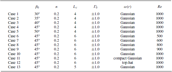
on the vortex sound generation. The parameters for the different configurations are listed in table 1. The initial inclination angle
 $\beta _0$
varies from
 $30^\circ$
to
 $50^\circ$
. The Reynolds number varies from 500 to 1000, considering the balance between the grid resolution and viscous dissipation according to the simulations reported in previous work (Kambe et al. Reference Kambe, Minota and Takaoka1993; Nakashima Reference Nakashima2008). The initial distance between the centres of the vortex rings is taken from
 $L_c=4$
to
 $L_c=6$
. The initial distribution of vorticity in the core is taken as Gaussian distribution, top-hat distribution or compact Gaussian distribution. The expressions of the three different initial distribution of vorticity are given as follows.
Parameters for the different configurations.

The Gaussian distribution of the initial vorticity field in the core is given by
 \begin{equation} \omega \left ( \xi \right ) =\omega _{G}\mathrm{exp}\left [ -\left ( \frac {\sigma }{\sigma _{0} } \right )^{2} \right ], \end{equation}
where
 $\omega _{G}$
is the maximum vorticity at the centre of the vortex core,
 $\xi$
is the distance from the axis of symmetry of vortex rings and
 $\sigma$
is the distance from the centre lines of vortex rings. The top-hat distribution of the initial vorticity field in the core is given by (Verzicco et al. Reference Verzicco, Iafrati, Riccardi and Fatica1997)
 \begin{align}& \omega \left ( \xi \right ) = \left \{ \begin{matrix} \omega _{t}\xi ,&\sigma \leqslant 0.8\sigma _0, \\ 1-f\left ( \eta \right ), &0.8\sigma _0 \lt \sigma \lt 1.2\sigma _0, \\ 0, & 1.2\sigma _0 \leqslant \sigma, \end{matrix}\right . \end{align}
 \begin{align}&\qquad\qquad\quad \eta = \frac {\sigma -0.8\sigma _0}{0.4\sigma _0}, \end{align}
where
 $\omega _{t}$
is the characteristic vorticity of the vorticity field following the tophat distribution and
 $r$
is the distance from the axis of symmetry of the vortex ring. The compact Gaussian distribution of the initial vorticity field in the core is given by (Daryan et al. Reference Daryan, Hussain and Hickey2020Reference Daryan, Hussain and Hickey2022)
 \begin{align} \omega \left ( \xi \right )& = \left \{ \begin{matrix} \omega _{c}\left (1-f\left ( \frac {\sigma }{\sigma _0} \right ) \right ),&\sigma \lt \sigma _0, \\[11pt] 0, &\sigma \geqslant \sigma _0, \end{matrix}\right .\\[-10pt]\nonumber \end{align}
 \begin{align} \sigma ^{2} &= \left (x-x_{c}\right )^{2}+\left (y-y_{c}\right )^{2}+\left (z-z_{c}\right )^{2},\\[-10pt]\nonumber \end{align}
 \begin{align} f\left ( \eta \right ) &= \exp \left ( { - K{\eta ^{ - 1}}{e^{\frac {1}{{\eta - 1}}}}} \right ),\quad K = \tfrac {1}{2}{e^2}\ln 2, \end{align}
where
 $\omega _{c}$
is the characteristic vorticity of the vorticity field following the compact Gaussian distribution and
 $x_c,y_c,z_c$
are the positions of the centre line of vortex rings. The three characteristic vorticity are determined by the principle of equalising the circulation of the vortex ring cross-sections
 $\Gamma _0$
, which is defined as
 $\Gamma _0=\pi \omega _{0} \sigma _{0}^{2}$
. Here,
 $\omega _{0}$
is the characteristic vorticity of the initial vorticity field and then the three characteristic vorticities are
 $\omega _{G}=31.83,\, \omega _{c}=114.60,\, \omega _{t}=62.82$
.
The initial velocity field is obtained via the Biot–Savart law,
 \begin{equation} \boldsymbol{u}=\frac {1}{4\pi } \int \frac {\boldsymbol{\omega } \times \boldsymbol{y}}{\left | \boldsymbol{y} \right | ^{3} }{\rm d}V . \end{equation}
The evolution of the solenoidal field associated with the vortex rings in the sound source region is governed by the three-dimensional unsteady Navier–Stokes equations for incompressible flows,
 \begin{align} \frac {\partial \boldsymbol{u} }{\partial t} + \bigtriangledown \cdot \left (\boldsymbol{u}\boldsymbol{u} \right ) & =-\bigtriangledown p + \frac {1}{Re} \bigtriangledown ^{2} \boldsymbol{u},\\[-10pt]\nonumber \end{align}
 \begin{align} \bigtriangledown \cdot \boldsymbol{u} & =0, \end{align}
where
 $\boldsymbol{u}$
denotes the non-dimensional velocity of the flow and
 $p$
is the non-dimensional pressure of the flow. We normalise all variables hereinafter. The reference length, velocity and density are
 $D_0$
,
 $\Gamma _0/D_0$
and
 $\rho _0$
, respectively, unless otherwise specified. The Reynolds number is defined as
 ${Re}=\Gamma _0/\nu$
, where
 $\nu$
is the kinematic viscosity of the fluid. The sound speed
 $c_0$
in (2.2) is determined by matching the Mach number associated with the initial translational velocity of the vortex ring. The Mach number is defined to
 $Ma=U_0/c_0$
and set to
 $0.1$
.
The Navier–Stokes equations are numerically solved by using a solver within the framework of OpenFOAM, where a second-order finite-volume method spatial discretisation and a second-order three step backward integration are used for the time advancement (Weller et al. Reference Weller, Tabor, Jasak and Fureby1998). The vorticity moments as the sources of the aerodynamics sound are computed by using a fourth-order Simpson method in a post-processing of the data . A fourth-order finite difference method is used for the time derivatives in computing the aerodynamic sound. The numerical methods for solving the Navier–Stokes equations and computing the aerodynamic sound are selected and tested in accordance with the work of Verzicco et al. (Reference Verzicco, Iafrati, Riccardi and Fatica1997).
Summary of the validations and assessment of this work.

The numerical simulation is conducted in a rectangular domain of
 ${y}_1\in [ 0,4.0 ]$
,
 ${y}_2\in [ 0,3.0 ]$
,
 ${y}_3\in [ -2.0,7.0 ]$
, which is a quarter of the whole domain. The comparisons between the results obtained in a quarter domain and in a whole domain are reported in Appendix B.2. It is noteworthy that using symmetry in the computational domain should be considered carefully when the Reynolds number increases, since the symmetry of the vortex ring might be broken at high Reynolds numbers (Yao & Hussain Reference Yao and Hussain2022). When symmetry breaking occurs, the use of symmetry of the computational domain will artificially enhance vortex stretching and, thus, the effect of the tilting. The periodic boundary condition is used in the
 $y_3$
-direction and symmetry boundary conditions are applied in the symmetry planes. Zero-gradient boundary conditions are adopted in the other planes. The domain is discretised on a mesh with
 $ 320\times 240\times 720$
grid points. The time step is set as
 $\Delta t/\Delta y_i=0.2$
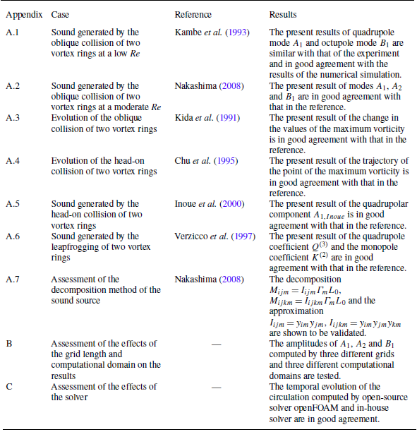
. The grid independence of the numerical set-up is tested in a similar simulation reported in Appendix B. The numerical method and set-up are validated by comparing the vortical flows of the vortex rings with the results of Kida et al. (Reference Kida, Takaoka and Hussain1991) and Chu et al. (Reference Chu, Wang, Chang, Chang and Chang1995), and comparing the sound generated by the leapfrogging and head-on collision of two vortex rings with the results of Verzicco et al. (Reference Verzicco, Iafrati, Riccardi and Fatica1997) and Inoue et al. (Reference Inoue, Hattori and Sasaki2000). The results are in good agreement with the references. All validations and assessments are summarised in table 2. The details of the validation of the numerical method and solver and the new vortex sound formula can be found in Appendix A. The oblique collision of vortex rings with the same initial configuration is also simulated by an in-house solver (Liu et al. Reference Liu, Wang, Wang and He2023) and the results are in good agreement, as reported in Appendix C.
5. Validation of the proposed vortex sound formula
We validate the proposed formula (3.1) in this section by comparing with the results of two reliable simulations:
 $(1)$
the sound pressure generated by the head-on collision of two vortex rings with equal initial strengths and radii in a viscous flow (Inoue et al. Reference Inoue, Hattori and Sasaki2000; Nakashima Reference Nakashima2008); and
 $(2)$
the sound pressure generated by the head-on collision of two vortex rings with unequal initial strengths in an ideal flow (Kambe & Minota Reference Kambe and Minota1981; Tang & Ko Reference Tang and Ko1995a
). The mutual cancellation and the effects of the consistency condition of vorticity moments on sound prediction are also reported in this section by comparing the robustness of sound calculations based on the vorticity field with Gaussian white noise.
5.1. Sound pressure generated by the head-on collision of two vortex rings in a viscous flow
We report the sound generated by the head-on collision of two vortex rings in a three-dimensional computational domain with the same configurations reported by Inoue et al. (Reference Inoue, Hattori and Sasaki2000) and Nakashima (Reference Nakashima2008) in this subsection. The initial vortex ring radii of the two vortex rings are equal and the initial circulations of the two vortex rings are opposite to each other. The initial vortex ring radius
 $R_0$
and the speed of sound
 $c_0$
in a quiescent medium are chosen as the characteristic variables. The ratio of core-to-ring radius is set as
 $n=0.30$
and the initial distance between two vortex rings is set as
 $L_c=16$
. The centres of vortex rings are located in
 $(0,\pm L_c/2,0 )$
, respectively. The initial inclination angle is
 $\beta =\pi /2.0$
and the vortex rings are perpendicular to the
 $y_2$
-axis. The initial distribution of vorticity in the core is taken as the Gaussian distribution defined in (4.2). The initial vorticity field in the vortex core is determined by the initial translational velocity of the vortex ring
 $U_0$
defined in (4.1) with the setting of
 $U_0=0.15$
. There are three symmetry planes for the geometry of the vortex rings during the head-on collision. Apart from the planes
 $(y_2,y_3), (y_1,y_3)$
, the velocity field is also symmetric about the plane
 $(y_1,y_2)$
. Therefore, the simulation can be conducted in a three-dimensional rectangular domain
 ${y}_1\in [ 0,8.0 ]$
,
 ${y}_2\in [ 0,11.0 ]$
,
 ${y}_3\in [ 0,8.0 ]$
, which is a one-eighth domain of the whole domain. The domain is discretised on
 $320\times 440\times 320$
grid points and the time step is
 $\Delta t=0.005$
. The Reynolds number is set as
 ${Re}=2300$
. The method used to discretise the Navier–Stokes equations are same as that in § 4. Symmetry boundary conditions are applied in the symmetry planes. Zero-gradient boundary conditions are adopted in the other planes.
The sound pressure is detected at
 $r=60$
and
 $\theta =\pi /2,\, \phi =\pi /2$
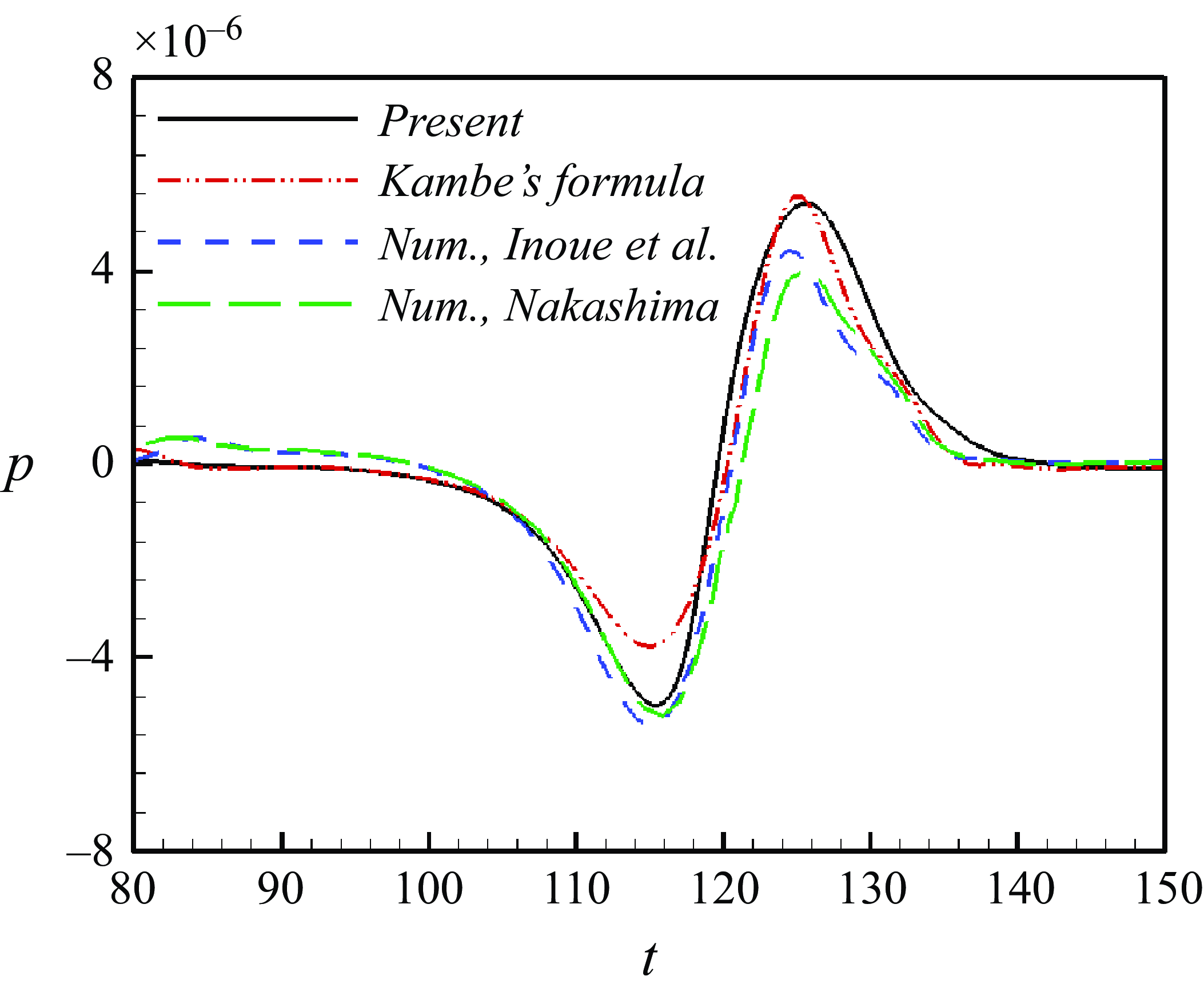
. Figure 3 shows the comparison between the sound pressure obtained by the proposed vortex sound formula (3.1) and that obtained by DNS of Inoue et al. (Reference Inoue, Hattori and Sasaki2000) and Nakashima (Reference Nakashima2008) at the observation point. The sound pressure has two pulses during the head-on collision of two vortex rings, where the first pulse is negative and the second pulse is positive. The peaks of the first negative pulse of the results obtained by the proposed vortex sound formula and DNS are almost equal. The difference between the results obtained by the proposed vortex sound formula and the reference might be caused by the application of vortex sound theory, since the similar difference between the sound pressure obtained by vortex sound theory and that obtained by DNS is also reported by Inoue et al. (Reference Inoue, Hattori and Sasaki2000). The results shown in figure 3 indicate that the proposed vortex sound formula can predict the sound generated by the interactions of vortex rings well.
Comparison between the sound pressure at
 $r_0=60$
obtained by the proposed vortex sound formula (3.1), Kambe’s formula (2.2), and the results of Inoue et al. (Reference Inoue, Hattori and Sasaki2000)and Nakashima (Reference Nakashima2008).

5.2. Sound pressure generated by the head-on collision of two vortex rings in a ideal flow
We report the sound generated by the head-on collision of two coaxial vortex rings in an ideal flow in this subsection. Dyson & Thomson (Reference Dyson and Thomson1893) proposed a thin vortex ring model to characterise the motion of vortex rings in radial and axial directions in an ideal flow. The ratio of core-to-ring radius
 $n$
is much smaller than
 $1$
, which represents that the radius of the vortex core is much smaller than the radius of the vortex ring. Vortex core remains circular during the interactions. The vorticity distributions in the vortex core are uniform. The vorticity field can be regraded as a concentrated vortex line with circulations
 $\Gamma _i$
passing through the vortex core centres
 $(Z_i, R_i)$
. The vorticity field can be defined as
 \begin{align} \boldsymbol{\omega } & =\left ( {0,{\omega _\theta },0} \right ), \end{align}
 \begin{align} \omega _{\theta , i} & = {\Gamma _i}\delta \left ( {r - {R_i}} \right )\delta \left ( {z - {Z_i}} \right ), \end{align}
where
 $\omega _\theta$
is the azimuth component in the vortex core and the subscript
 $i$
represents the first and second vortex ring.
The interaction between the vortex rings is manifested only by the induced velocity. The induced velocity
 $\boldsymbol{u}_i$
of vortex ring
 $i$
comprises two parts: the self-induced velocity from vortex ring
 $i$
and the mutual induced velocity from vortex ring
 $j$
(subscript
 $i,j$
representing the two vortex rings). Dyson & Thomson (Reference Dyson and Thomson1893) proposed an equation of the motion of two vortex rings,
 \begin{align} \frac {{{\rm d}{Z_i}}}{{{\rm d}t}} & = \frac {1}{{{R_i}}}\frac {{\partial \Psi _j }}{{\partial {R_i}}} + \frac {{{\Gamma _i}}}{{4\pi {R_i}}}\left [ {\log \left ( {\frac {{8{R_i}}}{{{\sigma _i}}}} \right ) - \frac {1}{4}} \right ], \end{align}
 \begin{align} \frac {{{\rm d}{R_i}}}{{{\rm d}t}} & = - \frac {1}{{{R_i}}}\frac {{\partial \Psi _j }}{{\partial {Z_i}}}, \end{align}
 \begin{align} \frac {d}{{\rm d}t}(\sigma _i^2{R_i}) & = 0. \end{align}
Here,
 $\Psi _j$
is the stream function associated with vortex ring
 $j$
,
 \begin{align}& \Psi = \frac {{{\Gamma _j}}}{{2\pi }}\sqrt {{R_i}{R_j}} \left [ {\left ( {\frac {2}{{{k_{ij}}}} - {k_{ij}}} \right )K\left ( {{k_{ij}}} \right ) - \frac {2}{{{k_{ij}}}}E\left ( {{k_{ij}}} \right )} \right ] ,\end{align}
 \begin{align}&\qquad\qquad {k_{ij}} = \sqrt {\frac {{4{R_i}{R_j}}}{{{{\left ( {{Z_i} - {Z_j}} \right )}^2} + {{\left ( {{R_i} + {R_j}} \right )}^2}}}}, \end{align}
where
 $K, E$
are the complete elliptic integrals of first and second kind, respectively. (5.2c
) indicates that the volume of each ring remains constant in time. Vortex stretching is taken into account by varying the radii of the vortex cores. The sound generated by the interactions of the vortex rings in an ideal flow can be obtained by (Kambe & Minota Reference Kambe and Minota1981)
 \begin{align} p \left ( \mathbf{x},t \right ) &=\frac {{{\rho _0}}}{{4c_0^2\left | \boldsymbol{x} \right |}}\frac {\partial ^3}{\partial t^3}Q \left ( t-\frac {\left | \boldsymbol{x} \right |}{c_{0} } \right )\left ( \cos ^2\alpha -\frac {1}{3} \right ), \end{align}
 \begin{align} Q \left ( t \right ) &= \iint z r^{2} \omega _{\theta } {\rm d}z{\rm d}r = \sum _{i}^{n} \Gamma _i R_i^2 Z_i ,\end{align}
where
 $\alpha$
represents the angle between the line connecting the acoustic observation point to the origin and the axial direction. Here,
 $n$
is the number of the vortex rings, and
 $R_i, Z_i$
represent the radial and axial positions of the vortex core centres that can be calculated by (5.2).
The head-on collision of two vortex rings is numerically simulated by solving (5.2) using a fourth-order Runge–Kutta method. The derivative of the stream function is solved using a second-order finite difference scheme. The model has been used to study the sound generated by the interactions of vortex rings (Kambe & Minota Reference Kambe and Minota1981). However, the model becomes invalid in the later stage of the head-on collision of two vortex rings with equal initial strengths and radii in an ideal flow. Therefore, we selected the sound pressure generated by the head-on collision of vortex rings with unequal initial strengths (Tang & Ko Reference Tang and Ko1995a
) as the benchmark case to assess the proposed formula’s performance. The circulation and radius of the first vortex ring
 $\Gamma _1, R_1$
are chosen as the characteristic variables. The initial circulation ratio
 ${\Gamma _2}/{\Gamma _1}$
is set as
 $-0.5$
and the initial radius ratio
 $ {R_2}/{R_1}$
is set as
 $1.0$
.
The three-dimensional flow field is constructed based on the circulations
 $\Gamma _i$
, radii
 $R_i$
, axial position
 $Z_i$
and the radii of vortex core
 $\sigma _i$
obtained by (5.2). The computational domain is a rectangular domain
 ${y}_1\in [ 7.5,14.0 ]$
,
 ${y}_2\in [ 0,2.5 ]$
,
 ${y}_3\in [ 0,2.5 ]$
, which is a one-eighth domain of the whole domain. The domain is discretised on
 $650\times 250\times 250$
grid points and the time step for the constructed flow field is
 $\Delta t=0.1$
. The sound pressure at
 $\left | \boldsymbol{x} \right |=60, \,\theta =\pi /2,\, \phi =\pi /2$
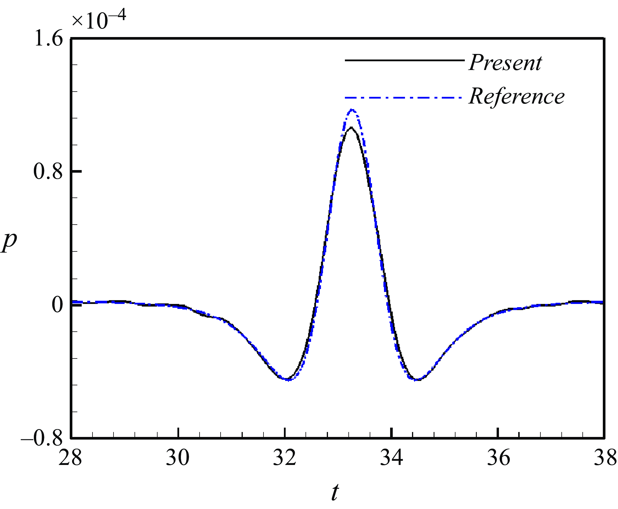
is calculated using (3.1) based on the constructed flow field. Figure 4 shows the comparison between the sound pressure obtained by the proposed vortex sound formula (3.1) and that obtained by (5.4). The difference in the peak values in the positive pulse between the sound pressure obtained by (3.1) and (5.4) is 8 %. The sound predicted by the proposed vortex sound formula is in good agreement with that predicted by the theory of vortex sound (5.4).


5.3. Effects of the consistency condition of vorticity moments on the sound prediction
We report the mutual cancellation and the effects of the consistency conditions of vorticity moments on sound prediction in this subsection by comparing the robustness of sound calculations based on the vorticity field with Gaussian white noise.
In § 3, the consistency conditions of vorticity moments are introduced to improve the coefficient of the lateral quadrupole mode
 $A_2$
, the coefficient of the longitudinal octupole mode
 $B_1$
and the coefficient of the lateral octupole mode
 $B_2$
. For example, the coefficient of the lateral quadrupole mode
 $A_2$
results from the linear combination of the vortical sources
 $M_{123}$
,
 $M_{132}$
and
 $M_{231}$
in (3.3b
). The contributions to the sound pressure of the lateral quadrupole component from the unit vortical sources
 $M_{123}$
,
 $M_{132}$
and
 $M_{231}$
cancelled each other out due to the consistency condition (3.4), which can be rewritten as
 $-(M_{132}+M_{231})=M_{123}$
,
 \begin{align} A_{2} & = \frac {\rho _{0}}{72\pi c_{0}^{2}r} \left (2M_{123}-(M_{132}+M_{231}) \right )^{(3)} \nonumber\\ & = \frac {\rho _{0}}{72\pi c_{0}^{2}r} \left (2M_{123} + M_{123} \right )^{(3)} = \frac {\rho _{0}}{24\pi c_{0}^{2}r} \left (M_{123} \right )^{(3)}. \end{align}
Therefore, the coefficient of the lateral quadrupole mode
 $A_2$
in (3.7b
) contains only the contribution from
 $M_{123}$
, and excludes the contributions from
 $M_{132}$
and
 $M_{231}$
. Additionally,
 $B_1$
and
 $B_2$
can be improved by combining (3.3) and (3.5),
 \begin{align} B_{1} &= \frac {\rho _{0}}{32\pi c_{0}^{3}r} \left [ \frac {4}{5}(M_{1332}-M_{2331})-\frac {1}{5}(M_{1112}+M_{1222}-M_{1121}-M_{2221}) \right ]^{(4)} \nonumber\\ &= \frac {\rho _{0}}{32\pi c_{0}^{3}r} \left [ \frac {4}{5}(M_{1332}-M_{2331})-\frac {1}{5}(-3M_{1121}-M_{1121}+M_{1222}+3M_{1222}) \right ]^{(4)} \nonumber\\ &= \frac {\rho _{0}}{40\pi c_{0}^{3}r} \left ( M_{1332}+M_{1121}-M_{2331}-M_{1222} \right )^{(4)},\\[-10pt]\nonumber \end{align}
 \begin{align} B_{2} &= \frac {\rho _{0}}{960\pi c_{0}^{3}r} \left (4M_{1233}+ M_{1112}+M_{2221}-M_{1121}-M_{1222}-2M_{1332}-2M_{2331} \right )^{(4)} \nonumber\\ &= \frac {\rho _{0}}{960\pi c_{0}^{3}r} \left (2(2M_{1233}-M_{1332}-M_{2331}) + (M_{1112}-M_{1121})+(M_{2221}-M_{1222}) \right )^{(4)} \nonumber\\ &= \frac {\rho _{0}}{240\pi c_{0}^{3}r} (2M_{1233}-M_{1121}-M_{1222})^{(4)}. \end{align}
Figure 5 shows the comparison of
 $A_2, B_1, B_2$
obtained by Kambe’s formula (3.3) and the proposed formula (3.7). The curves of
 $A_2, B_1, B_2$
essentially overlap. The results indicate that the consistency conditions of vorticity moments are valid in this work.


The consistency conditions of vorticity moments can cancel the spurious sound that comes from numerical or experimental errors. We take the assessment of the consistency condition of the second moments of vorticity given by (3.4) in a perturbed vorticity field as an example. The perturbed vorticity field is constructed by adding Gaussian white noise to the vorticity field in Case 10. The mean and variance of Gaussian white noise are set as 0 and 1, respectively. Figure 6 shows the consistency condition of the second moments of vorticity given by (3.4) during the oblique collision of two vortex rings in the perturbed and unperturbed vorticity fields. It is shown that the perturbed vorticity field does not satisfy the consistency condition of vorticity moments given by (3.4). The inconsistency of the perturbed vorticity will introduce significant errors in sound prediction. Imposing the consistency condition on the coefficient functions can enhance its conservation properties and reduce the sensitivity to errors. Figure 7 shows the comparisons of the coefficient functions of the spherical harmonic modes
 $A_2, B_1, B_2$
obtained by (3.7) and (3.3) based on the vorticity field with Gaussian white noise. The results obtained by (3.7) exhibit significantly less dispersion than those obtained by (3.3). It indicates that the consistency conditions of vorticity moments can eliminate the spurious sound.
6. Results and discussion
In this section, we report on and discuss the sound pressure and vortical flows generated by the oblique collision of two vortex rings. The sound pressure in the far field is reported and discussed in § 6.1, where three dominant modes are identified: the longitudinal quadrupole mode, the lateral quadrupole mode and the longitudinal octupole mode. The evolution of the vortical flows in the source region during the collision is described in § 6.2. The relation between the far-field sound pressure and the vortical flows in the source region are discussed in § 6.3.
Assessment of the consistency condition of the second moments of vorticity given by (3.4) in a perturbed vorticity field.

Time evolutions of (a) the coefficient of the lateral quadrupole mode
 $A_2$
, (b) the coefficient of the longitudinal octupole mode
 $B_1$
and (c) the coefficient of the lateral octupole mode
 $B_2$
based on the vorcity field with Gaussian white noise.

6.1. Sound pressure in the far field
The sound pressure radiated from the oblique collision of a pair of vortex rings is featured by the asymmetric emission. The asymmetric emission can be clearly seen from figure 8, where a typical instantaneous sound pressure field on the plane
 $(y_{1},y_{3})$
is shown. The sound pressure is computed by using the vortex sound formula (2.1) with the vortical flows in Case 10. The sound pressure field is symmetric with respect to the
 $y_1$
-axis, but asymmetric with respect to the
 $y_3$
-axis. The longitudinal octupole mode is asymmetric with respect to the
 $y_3$
-axis, while the longitudinal and lateral quadrupole modes are symmetric with respect to the
 $y_3$
-axis, as shown in figures 8(b)–8(d). Therefore, the asymmetry of sound pressure field results from the longitudinal octupole mode.
(a) Sound pressure generated by the interaction of vortex rings in Case 10, and three modes (b)
 $A_{1}$
, (c)
 $A_{2}$
and (d)
 $B_{1}$
on the plane
 $(y_{1},y_{3})$
at
 $t'=4.23$
.

The typical evolution of the root mean square (r.m.s.) of the pressure
 $p_{{rms}}$
is shown in figure 9, where the non-dimensional
 $p_{{rms}}$
on a spherical surface with
 $r_0 = 100 D_0$
corresponding to Case 10 is shown. Here, we present the sound pressure in the source time
 $t$
instead of the retarded time
 $t^* = t - r_0/c_0$
, for the convenience of analysing the evolution of the sources of aerodynamic sound. The r.m.s. of the non-dimensional pressure
 $p_{{rms}}$
is computed by
 \begin{equation} p_{{rms}} = \sqrt {\frac {\sum _{i=0}^{N} {(p_{i} - p_m)}^{2} }{N} }, \end{equation}
where
 $N=40\,000$
is the number of sampling points in this work,
 $p_i$
is the sound pressure obtained from (2.1) at the
 $i$
th sampling point and
 $p_m$
is the mean sound pressure on the spherical surface. The r.m.s. of the pressure has three pulses during the oblique collision, but the acoustic power is dominated by the first two pulses. For example, the three peaks of
 $p_{{rms}}$
for the configuration of Case 10 are
 $ 3.84\times 10^{-7}$
,
 $7.25\times 10^{-7}$
and
 $1.78\times 10^{-7}$
, respeectively. The ratio between the three peaks is
 $2:4:1$
. The acoustic power
 $\Pi$
scales with
 $p_{{rms}}^2$
. Therefore, the first and second pulses of
 $p_{{rms}}$
cause two large pulses in acoustic power, while the third pulse of
 $p_{{rms}}$
corresponds to a relatively low acoustic power, as shown in figure 9(b). The temporal evolution the acoustic power is consistent with the results of Nakashima (Reference Nakashima2008).
The sound pressure generated by the oblique collision of two vortex rings depends on the initial inclination angle
 $\beta _0$
, the Reynolds number
 ${Re}$
, the initial distance between the centres of the vortex rings
 $L_c$
, the initial distribution of vorticity field in the vortex core
 $\omega (r)$
on the vortex sound generation, as well as the ratio of core-to-ring radius
 $n$
. The investigation on the coaxial collision of two vortex rings shows that the relatively thick vortex rings do not present particular features. The thin vortex rings (
 $n=0.15$
) lead to an active vortex interaction that is closer to the inviscid ‘leapfrogging’. The other effect of the ratio of core-to-ring radius on the sound generation is that it influences the vorticity gradient within the core (Verzicco et al. Reference Verzicco, Iafrati, Riccardi and Fatica1997). The ‘leapfrogging’ is absent in the oblique collision of two vortex rings. The influences of the vorticity gradient within the core can be reflected by changing the initial distribution of vorticity within the core. Therefore, this work focuses on the effects of the first four parameters on the sound pressure.
Temporal evolution of (a) the root-mean-square of sound pressure
 $p_{{rms}}$
and (b) the acoustic power of Case 10 at
 $r_0=100D_0$
.

Time-dependent acoustic power generated by two vortex rings with different (a) initial inclination angles, (b) Reynolds numbers, (c) initial distance and (d) initial distributions of vorticity in the core.

Figure 10 shows the acoustic power radiated by the oblique collision under different initial configurations. The time dependent acoustic power is dominated by two pulses in all the cases investigated in this work. When the initial inclination angle increases from
 $30^\circ$
to
 $50^\circ$
, the maximum peaks of the acoustic power increases from
 $ 0.84\times 10^{-7}$
to
 $ 3.95\times 10^{-7}$
, as shown in figure 10(a). The acoustic power of the case with large initial inclination angle reaches maximum earlier than that with the small one. The increasing of acoustic power with the increase of the initial inclination angle is consistent the results of Nakashima (Reference Nakashima2008), although the ranges of the initial inclination are different. When the Reynolds number increases from
 $500$
to
 $1000$
, the maximum peaks of the acoustic power increases from
 $ 5.3\times 10^{-9}$
to
 $ 8.5\times 10^{-8}$
, as shown in figure 10(b). The instant at which the acoustic power peaks was slightly affected by the Reynolds number. When the initial distance between the centres of the vortex rings increases from
 $4.0D_0$
to
 $6.0D_0$
, the maximum peaks of the acoustic power increases from
 $ 0.77\times 10^{-7}$
to
 $ 3.01\times 10^{-7}$
, as shown in figure 10(c). Figure 10(d) shows the time-dependent acoustic power when the initial distributions of vorticity in the core are taken as the Gaussian distribution, top-hat distribution and compact Gaussian distribution. The different initial vorticity distributions corresponds to different vorticity gradients within the core. The maximum acoustic power increases with the increase of vorticity gradient.
Temporal evolution of the acoustics power under all different initial configurations.

The normalised power
 $\Pi '$
and time
 $t'$
are the combinations of a few non-dimensional variables. These variables include
 \begin{align}\Pi ' & = \Pi /\big({\beta ^{3.0}}{( {Re/1000})^4}\omega _0^{0.6}L_c^{ - 3}\big),\\[-10pt]\nonumber \end{align}
 \begin{align} t' & = t/\big({\beta ^{0.75}}{ {R}}{ {e}}^{ - 0.125}\omega _0^{ - 0.1}L_c^{1.25}\big), \end{align}
where
 $\omega _0$
is the non-dimensional vorticity that can be replaced by the characteristic vorticity in the Gaussian distribution
 $\omega _G$
, the top-hat distribution
 $\omega _t$
and the compact Gaussian distribution
 $\omega _c$
. Here,
 $L_c$
is the non-dimension initial distance and is normalised by
 $D_0$
. The curves of the
 $\Pi '$
against
 $t'$
almost collapse, as shown in figure 11 .
Since the evolution of the vortex rings and the aerodynamic sound power depend on all the above mentioned non-dimensional variables, we renormalised the aerodynamic sound power and time by multiplying the non-dimension variables with different powers. The motivation of the renormalisation is to show the similarity of generating aerodynamic sound in different configurations. The renormalisation is inspired by the work of Inoue et al. (Reference Inoue, Hattori and Sasaki2000) and Kambe & Minota (Reference Kambe and Minota1983) in investigating the co-axial collisions of a pair of vortex rings. We would like to note that caution should be paid to extrapolate the current scaling laws (Stumpf & Porter Reference Stumpf and Porter2012).
6.2. Vortical flows in the source region
The oblique collisions investigated in this work have similar vortical flow pattern. We use the evolution of the vortical flows in Case 10 to illustrate the features of vortex dynamics in the oblique collision. The typical evolution of the vortical flows is presented in figure 12, where the iso-surface of vorticity magnitude is plotted. We divided the evolution of the vortical flows into three stages, in accordance with the r.m.s. of pressure in figure 9(a).
Evolution of vortex rings in the oblique collision in Case 10 at (a)
 $t^{\prime} = 1.95$
, (b)
 $t^{\prime} = 3.25$
, (c)
 $t^{\prime} = 3.66$
, (d)
 $t^{\prime} = 3.98$
, (e)
 $t^{\prime} = 4.39$
, (f)
 $t^{\prime} = 4.79$
, (g)
 $t^{\prime} = 5.61$
, (h)
 $t^{\prime} = 6.01$
, (i)
 $t^{\prime} = 7.23$
. The vortex rings are represented by the isosurfaces of
 $\omega _0/10$
. The isosurfaces are coloured with vorticity in the collision direction.

Line connecting the peaks of
 $\omega _2$
on the plane
 $(y_{1},y_{3})$
and the oblique angle
 $\beta$
at (a)
 $t^{\prime} = 2.03$
, (b)
 $t^{\prime} = 4.47$
, (c)
 $t^{\prime} = 5.12$
.

Temporal evolution of the angle between the vortex rings and the
 $y_1$
axis.

Evolution of the isosurfaces of 10 % of maximum initial vorticity magnitude and vortex lines at (a)
 $t^{\prime} = 3.82$
, (b)
 $t^{\prime} = 4.14$
, (c)
 $t^{\prime} = 4.47$
, (d)
 $t^{\prime} = 5.12$
, (e)
 $t^{\prime} = 6.09$
, (f)
 $t^{\prime} = 7.31$
. The isosurfaces and lines are shaded with contours of vorticity in the collision direction.

In the first stage, each vortex ring approximately advects along the direction parallel to the axis (the symmetry axis of each vortex ring). The geometry and inclination angle of the vortex rings are mainly unchanged except at the end of this stage, as shown in figures 12(a)–12(c). The inclination angle of the vortex rings can be represented by the distribution of the vorticity
 $\omega _2$
on the plane (
 $y_1$
,
 $y_3$
). We use the time dependent tilting angle
 $\beta (t)$
to measure the tilting of the right vortex ring. Here, the tilting angle
 $\beta$
is defined as the angle between the
 $y_1$
-axis and the line connecting the peaks of
 $\omega _2$
of the right vortex ring, as shown in figure 13. The tilting angle
 $\beta (t)$
is approximately the initial inclination angle
 $\beta _0 = 45^{\circ }$
during this stage, as shown in figure 14.
In the second stage, the lower parts of the vortex rings collide and reconnect on the plane (
 $y_2$
,
 $y_3$
), and the upper parts keep moving towards each other, as shown in figures 12(d)–12(f). The motion of the upper parts of the vortex rings causes a rapid increase in the inclination angle
 $\beta (t)$
, which increases from
 $\beta = 56^{\circ }$
at
 $t'=3.8$
to
 $\beta = 82^{\circ }$
at
 $t'=5.0$
, as shown in figure 14. This rapid change in the tilting of the vortex ring is a distinctive feature of the oblique collision of vortex rings, which is absent in the coaxial interaction of vortex rings. Another distinctive feature of oblique collision is the vortex reconnection, as shown in figure 15. The vortex reconnection can be identified using the vorticity along the collision direction
 $\omega _1$
on the collision plane (
 $y_2$
,
 $y_3$
). The vorticity along the collision direction
 $\omega _1$
on the collision plane (
 $y_2$
,
 $y_3$
) is zero before the vortex rings reconnect to each other. The connection of vorticity lines between the two vortex rings results in the generation of
 $\omega _1$
on the collision plane (
 $y_2$
,
 $y_3$
), as shown in figure 16. We use a circulation
 $\gamma _{1}$
corresponding to the vorticity component
 $\omega _1$
on the collision plane (
 $y_2$
,
 $y_3$
) to measure the vortex reconnection. Here, the circulation
 $\gamma _{1}$
is defined as
 \begin{equation} \gamma _{1} = \int _S \omega _1 {\rm d}S , \end{equation}
where
 $S$
is the plane defined by
 $\phi = 3/2\pi$
. Figure 17 shows the variation of the circulation
 $\gamma _{1}$
during the collision. The vortex reconnection starts from
 $t' = 3.82$
, when
 $\gamma _{1}$
reaches 5 % of
 $\Gamma _0$
, according to the criterion used in the literature (Daryan et al. Reference Daryan, Hussain and Hickey2020, Reference Daryan, Hussain and Hickey2022; Yao & Hussain Reference Yao and Hussain2022). The circulation
 $\gamma _{1}$
increases monotonically as the vortex lines in one vortex ring connect to those in the other vortex ring, as shown in figures 15(b)– 15(d).
Contours of vorticity in the collision direction on the plane
 $(y_{2},y_{3})$
at different time (a)
 $t^{\prime} = 3.82$
, (b)
 $t^{\prime} = 4.79$
, (c)
 $t^{\prime} = 5.61$
.

Temporal evolution of the circulation on the plane of
 $ ( y_2,y_3 )$
.

In the third stage, the remnant vorticity after collision forms a highly deformed vortex ring with two parallel arched vortex tubes, as shown in figures 12(g)–12(i). The tilting angle of the vortex ring is mainly unchanged, as shown in figures 15(e)–15(f) and the tilting angle
 $\beta$
tends towards
 $90^{\circ }$
, as shown in figure 14. The circulation
 $\gamma _{1}$
reaches a maximum at
 $t' = 5.93$
and then decays, as shown in figure 17.
The reconnecting of vortex rings in the second stage is accompanied with the significant tilting of the vortex rings. While the reconnecting of vortex rings in the oblique collision of two vortex rings has been investigated in detail in the work of Kida et al. (Reference Kida, Takaoka and Hussain1991) and Nakashima (Reference Nakashima2008), this work focuses on the tilting of the vortex rings. We use the equivalent circulation corresponding to the vorticity in the collision direction (
 $\Gamma _1$
) defined by (3.9) to quantitatively investigate the contribution of the tilting of vortex rings. The variation of the equivalent circulation
 $\Gamma _1$
results from the tilting, deforming and reconnecting of the vortex rings. We decompose the equivalent circulation
 $\Gamma _1$
into the contributions from the tilting of an ideal vortex ring
 $\Gamma _{10}$
and the correction from the deforming the reconnecting
 $\Gamma _{1c}$
,
 \begin{align} \Gamma _{1} (t) & = \frac {1}{L_0} \int _\Omega \omega _1 (t) {\rm d}v \end{align}
 \begin{align} & = \frac {1}{L_0} \int _\Omega \omega _{10} (t) {\rm d}v + \frac {1}{L_0} \int _\Omega \left ( \omega _{1} (t) - \omega _{10} (t)\right ) {\rm d}v \end{align}
 \begin{align} & \triangleq \Gamma _{10}(t) + \Gamma _{1c} (t), \end{align}
where
 $\omega _{1} (t)$
is the time-dependent vorticity in the collision direction,
 $\omega _{10} (t)$
is the time-dependent vorticity in the collision direction contributed by the tilting of an ideal vortex ring. The ideal vortex rings are taken as the initial vortex rings reported in § 2.1 and the tilting angle
 $\beta (t)$
is taken as that shown in figure 14. Here,
 $\omega _{1} (t) - \omega _{10} (t)$
represents the deviation of the vorticity from the ideal vortex ring due to the reconnecting and deforming.
Temporal evolution of the equivalent circulation in comparation with that caused by the change of orientation in the collision direction.

Figure 18 shows the variation of the equivalent circulation
 $\Gamma _1$
during the collision of Case 10, where the variations of the equivalent circulation associated with the changes in tilting
 $\Gamma _{10}$
and that associated with the reconnecting and deforming
 $\Gamma _{1c}$
are also plotted. In the first stage (
 $2.0 \lt t' \lt 3.8$
), the equivalent circulation mainly results from the tilting of the vortex ring, since
 $\Gamma _1 \approx \Gamma _{10}$
during the most part of this stage. Here,
 $\Gamma _{10}$
slightly deviates from
 $\Gamma _1$
at the end of this stage. This deviation is mainly caused by the deformation of the vortex rings, since the vortex reconnection starts from
 $t'=3.82$
, according to the criterion used in the literature (Daryan et al. Reference Daryan, Hussain and Hickey2020, Reference Daryan, Hussain and Hickey2022; Yao & Hussain Reference Yao and Hussain2022). In the second stage (
 $3.8 \lt t' \lt 5.0$
), the change in equivalent circulation
 $\Gamma _1$
is contributed by both the vortex ring tilting and the deviation of vorticity from the initial distribution, where the deviation is caused by the reconnecting and deforming of the vortex rings. In the third stage (
 $5.0 \lt t' \lt 8.0$
), the tilting of vortex rings tends to
 $90^{\circ }$
and the variation of the equivalent circulation is dominated by the vortex deformation and reconnection.
Temporal evolution of the first-order time derivative of the equivalent circulation (a)
 $\Gamma _{1}^{(1)}$
and its (b) second-order time derivative
 $\Gamma _{1}^{(2)}$
, (c) third-order time derivative
 $\Gamma _{1}^{(3)}$
, (d) forth-order time derivative
 $\Gamma _{1}^{(4)}$
.

Both
 $\Gamma _{10}$
and
 $\Gamma _{1c}$
contribute to the equivalent circulation
 $\Gamma _{1}$
. The tilting of vortex rings (
 $\Gamma _{10}$
) tends to reduce the magnitude of
 $\Gamma _{1}$
, while the reconnecting and deforming (
 $\Gamma _{1c}$
) tends to increase it. The different tendencies can be clearly seen by taking the derivative of
 $\Gamma _{10}$
and
 $\Gamma _{1c}$
with respect to time, as shown in figure 19. All the first- to fourth-order derivatives of
 $\Gamma _{10}$
are almost out of phase with those of
 $\Gamma _{1c}$
, which indicates that the variation of the equivalent circulation caused by
 $\Gamma _{1c}$
is compensated by that caused by
 $\Gamma _{10}$
. As will be discussed in § 6.3, the time derivatives of the equivalent circulation
 $\Gamma _{1}$
contribute the most part of the aerodynamic sound. The compensation of
 $\Gamma _{10}$
to
 $\Gamma _{1c}$
indicates that the vortex tilting reduces the aerodynamic sound generated by reconnecting and deforming.
6.3. Relation between the sound pressure and vortical flows
The oblique collisions investigated in this work have similar sound pressure features and vortical flow patterns. Therefore, we use the configuration of Case 10 as a typical case to discuss the relation between the sound pressure and vortical flows. Figure 20 shows the temporal evolution of the five coefficients
 $A_0$
,
 $A_1$
,
 $A_2$
,
 $B_1$
and
 $B_2$
in (2.1) at a distance of
 $r_0=100D_0$
. The coefficient of the longitudinal quadrupole mode
 $A_1$
has the maximum peaks. The
 $A_1$
is featured by a negative peak in the first stage (
 $S_{\textrm{I}}$
,
 $2.0 \lt t' \lt 3.8$
) and a positive peak in the second stage (
 $S_{\textrm{II}}$
,
 $3.8 \lt t' \lt 5.0$
). The peak values and the corresponding time are listed in table 3. The coefficient of the lateral quadrupole mode
 $A_2$
reaches the negative peak and positive peak at almost the same time as
 $A_1$
. The magnitudes of the peaks of
 $A_2$
are approximately one-third of those of
 $A_1$
. The coefficient of the longitudinal quadrupole mode
 $B_1$
also has a negative peak in the first stage and a positive peak in the second stage. The magnitudes of the peaks of
 $B_1$
is of the same order of the peak of
 $A_2$
. The magnitudes of the monopole mode coefficient
 $A_0$
and the lateral octapole mode coefficient
 $B_2$
are much smaller than those of
 $A_1$
.
Temporal evolution of the five coefficients of the different modes in (2.1) at
 $r_0=100D_0$
.

Peak values and the instant corresponding the peak values of the five modes.

The abovementioned results indicate that the sound generated by the oblique collision of vortex rings is dominated by three modes: the longitudinal quadrupole mode, the lateral quadrupole mode and the longitudinal octupole mode. The analyses according to (3.1) reveal that the longitudinal quadrupole and octupole modes are mainly contributed by the variation of the circulation associated with the tilting of the vortex rings, while the lateral quadrupole mode is mainly contributed by the jerk of the vorticity centriod associated with the deformation and reconnection. Considering that this work focuses on the tilting of the vortex ring, we report the analyses of the longitudinal quadrupole and octupole modes in detail in §§ 6.3.1 and 6.3.2, respectively. The analyses of the lateral quadrupole mode are briefly discussed in Appendix D.
6.3.1. Longitudinal quadrupole mode
The coefficient
 $A_1$
in (3.1) depends on the third-order time derivative of the vorticity moments
 $( y_{12}y_{32}\Gamma _2 )^{(3)}$
and
 $-( y_{21}y_{31}\Gamma _1 )^{(3)}$
, according to (3.1a
). Figure 21 shows the temporal evolution of
 $( y_{12}y_{32}\Gamma _2 )^{(3)}$
and
 $-( y_{21}y_{31}\Gamma _1 )^{(3)}$
, as well as the re-scaled coefficient of the longitudinal quadrupole mode
 $ A_{1}^{*}=A_1/(\rho _{0}/(12\pi c_{0}^{2}r_0))$
. In the first stage (
 $S_{\textrm{I}}$
,
 $2.0 \lt t' \lt 3.8$
),
 $-( y_{21}y_{31}\Gamma _1 )^{(3)}$
reaches the same negative peak as the re-scaled coefficient
 $ A_{1}^{*}$
at
 $t'=3.62$
. In the second stage (
 $S_{\textrm{II}}$
,
 $3.8 \lt t' \lt 5.0$
),
 $-( y_{21}y_{31}\Gamma _1 )^{(3)}$
reaches the positive peak at the same time as the re-scaled coefficient
 $ A_{1}^{*}$
. The positive peak of
 $-( y_{21}y_{31}\Gamma _1 )^{(3)}$
is 0.026, which contributes 77 % of that of
 $ A_{1}^{*}$
. The results reveal that the variation of
 $A_1$
is dominated by
 $-( y_{21}y_{31}\Gamma _1 )^{(3)}$
. Therefore, the relationship between the peaks of the coefficient
 $A_1$
and the evolution of the vorticity can be investigated by analysing the third-order time derivative of the vorticity moment
 $-( y_{21}y_{31}\Gamma _1 )^{(3)}$
.
Temporal evolution of the fluctuation part of the amplitude of quadrupole and two components.

Temporal evolution of geometrical indexes (a)
 $y_{21}y_{31}$
and its (b) first-order time derivative
 $(y_{21}y_{31})^{(1)}$
, (c) second-order time derivative
 $(y_{21}y_{31})^{(2)}$
, (d) third-order time derivative
 $(y_{21}y_{31})^{(3)}$
.

The third-order time derivative of the vorticity moment
 $-( y_{21}y_{31}\Gamma _1 )^{(3)}$
can be decomposed into four terms as follows:
 \begin{equation} \frac {-( y_{21}y_{31}\Gamma _1 )^{(3)}}{L_0} = \underbrace {-{( y_{21}y_{31} )}\Gamma _1^{(3)}}_{T_1} \underbrace {-3( y_{21}y_{31} )^{(1)}\Gamma _1^{(2)}}_{T_2} \underbrace {-3( y_{21}y_{31} )^{(2)}\Gamma _1^{(1)}}_{T_3} \underbrace {-( y_{21}y_{31} )^{(3)}\Gamma _1}_{T_4}. \end{equation}
The first term
 $T_1$
on the right-hand side of (6.5) mainly represents the contribution from the third-order time derivative of the equivalent circulation
 $\Gamma _1^{(3)}$
, since the third-order time derivative of
 $\Gamma _1^{(3)}$
rises or declines more steeply than
 $ y_{21}y_{31}$
during the collision, as shown in figures 19(c) and 22(a), respectively. Similarly, the fourth term
 $T_4$
mainly represents the contribution from the third-order time derivative of the vorticity-weighted product of inertia
 $( y_{21}y_{31} )^{(3)}$
. The second term
 $T_2$
and the third term
 $T_3$
represent the interaction between the time derivatives of the equivalent circulation and the vorticity-weighted product of inertia. Figure 23 shows the temporal evolution of the four terms in (6.5) .
Temporal evolution of these four components to the dominant term of the longitudinal quadrupole mode.

In the first stage, the first term
 $T_1$
on the right-hand side of (6.5) has a negative peak, as shown in figure 23. This peak is caused by the variation of the equivalent circulation
 $\Gamma _1$
, since the third-order derivative of the equivalent circulation
 $\Gamma _1^{(3)}$
has a peak at
 $t'=3.74$
and the vorticity-weighted product of inertia
 $y_{21}y_{31}$
increases monotonically in this stage, as shown in figures 19(c) and 22(a), respectively. The contribution from the fourth term
 $T_4$
increases monotonically and is diminished by the other terms. Therefore, the negative peak of
 $-( y_{21}y_{31}\Gamma _1 )^{(3)}$
in the first stage mainly results from the variation of the circulation associated with the first term
 $T_1$
in (6.5).
In the second stage, the first term
 $T_1$
has a positive peak at the same time that
 $-( y_{21}y_{31}\Gamma _1 )^{(3)}$
reaches its maximum, as shown in figures 21 and 23. This peak is also caused by the variation of the equivalent circulation
 $\Gamma _1$
, since the third-order derivative of the equivalent circulation
 $\Gamma _1^{(3)}$
has a peak at
 $t'=4.22$
and the vorticity-weighted product of inertia
 $y_{21}y_{31}$
increases monotonically in this stage, as shown in figures 19(c) and 22(a), respectively. Similar to that in the first stage, the contributions from the fourth term
 $T_4$
is diminished by
 $T_2$
and
 $T_3$
terms.
These results reveal that the peaks of the longitudinal quadrupole mode coefficient
 $A_1$
in both the first and second stages are mainly caused by the equivalent circulation
 $\Gamma _1^{(3)}$
. As reported in § 6.2, the time-dependent equivalent circulation
 $\Gamma _1^{(3)}$
is contributed both by
 $\Gamma _{10}^{(3)}$
associated with the tilting of vortex rings and
 $\Gamma _{1c}^{(3)}$
associated with the reconnecting and deforming of the vortex ring. The contribution of
 $\Gamma _{1c}^{(3)}$
is compensated by
 $\Gamma _{10}^{(3)}$
, due to the nearly out of phase between the two lines, as shown in figure 19(c). Therefore, the tilting of the vortex ring reduces the longitudinal quadrupole mode.
Temporal evolution of the four terms in the coefficient of longitudinal octupole mode.

Temporal evolution of geometrical indexes (a)
 $( y_{21}y_{31}^2 )$
and its (b) first-order time derivative
 $( y_{21}y_{31}^2 )^{(1)}$
, (c) second-order time derivative
 $( y_{21}y_{31}^2 )^{(2)}$
, (d) third-order time derivative
 $( y_{21}y_{31}^2 )^{(3)}$
, (e) fourth-order time derivative
 $( y_{21}y_{31}^2 )^{(4)}$
, and (e) comparison with the product of vorticity centroid
 $I_{2331}-y_{21}y_{31}^{2}$
.

Temporal evolution of these five components to the dominant term of the longitudinal octupole mode.

6.3.2. Longitudinal octupole mode
The coefficient
 $B_1$
in (3.1) depends on the fourth-order time derivatives of the vorticity moments
 $( y_{12}y_{32}^2\Gamma _2 )^{(4)}$
,
 $( y_{11}^2y_{21}\Gamma _1 )^{(4)}$
,
 $-( y_{21}y_{31}^2\Gamma _1 )^{(4)}$
and
 $-( y_{12}y_{22}^2\Gamma _2 )^{(4)}$
, according to (3.7). Figure 24 shows the contribution to the coefficient
 $B_1$
from the four terms. The contribution from
 $-( y_{21}y_{31}^2\Gamma _1 )^{(4)}$
dominates the both the negative peak in the first stage and the positive peak in the second stage. We analyse the relationship between the peaks of the coefficient
 $B_1$
and the evolution of the vorticity by decomposing the fourth-order time derivative of the vorticity moment
 $-( y_{21}y_{31}^2\Gamma _1 )^{(4)}$
.
The fourth-order time derivative of the vorticity moment
 $( y_{21}y_{31}^2\Gamma _1 )^{(4)}$
can be decomposed into five terms as follows:
 \begin{eqnarray} \begin{split} \frac {-( y_{21}y_{31}^2\Gamma _1 )^{(4)}}{L_0} = & \underbrace {-{( y_{21}y_{31}^2 )}\Gamma _1^{(4)}}_{C_1} \underbrace {-4( y_{21}y_{31}^2 )^{(1)}\Gamma _1^{(3)}}_{C_2} \underbrace {-6( y_{21}y_{31}^2 )^{(2)}\Gamma _1^{(2)}}_{C_3} \\ & \underbrace {-4( y_{21}y_{31}^2 )^{(3)}\Gamma _1^{(1)}}_{C_4} \underbrace {-( y_{21}y_{31}^2 )^{(4)}\Gamma _1}_{C_5}. \end{split} \end{eqnarray}
The first term
 $C_1$
on the right-hand side of (6.6) mainly represents the contribution from the fourth-order time derivative of the equivalent circulation
 $\Gamma _1^{(4)}$
, since the fourth-order time derivative of
 $\Gamma _1^{(4)}$
rises or declines more steeply than
 $ y_{21}y_{31}^2$
during the collision, as shown in figures 19(d) and 25(a), respectively. Similarly, the fifth term
 $C_5$
mainly represents the contribution from the fourth-order time derivative of the geometrical index
 $( y_{21}y_{31}^2 )^{(4)}$
. The other terms,
 $C_2$
,
 $C_3$
and
 $C_4$
, represent the interaction between the time derivatives of the equivalent circulation and the vorticity-weighted geometrical index of the vortex ring. Figure 26 shows the temporal evolution of the five terms in (6.6).
In the first stage, the first term
 $C_1$
on the right-hand side of (6.6) has a negative peak. This peak is caused by the variation of the circulation, since the fourth-order derivative of the equivalent circulation
 $\Gamma _1^{(4)}$
has a peak at
 $t'=3.57$
and the vorticity-weighted geometrical index
 $( y_{21}y_{31}^2 )$
increases monotonically in this stage, as shown in figures 19(d) and 25(a), respectively. The second term
 $C_2$
on the right-hand side of (6.6) has also a negative peak in this stage. The negative peak of
 $C_2$
is caused by the third-order derivative of the equivalent circulation
 $\Gamma _1^{(3)}$
, since
 $\Gamma _1^{(3)}$
has a peak at
 $t'=3.74$
. The fifth term
 $C_5$
has positive values, but its contribution is compensated by the combination of the other four terms. Therefore, the negative peak of
 $-( y_{21}y_{31}^2\Gamma _1 )^{(4)}$
in the first stage mainly caused by the peaks of
 $\Gamma _1^{(4)}$
and
 $\Gamma _1^{(3)}$
.
In the second stage, the positive peak of
 $-( y_{21}y_{31}^2\Gamma _1 )^{(4)}$
also mainly results from the contribution of the first term
 $C_1$
and the second term
 $C_2$
on the right-hand side of (6.6). The first term
 $C_1$
reaches a positive peak at the time which
 $-( y_{21}y_{31}^2\Gamma _1 )^{(4)}$
reaches its maximum. The positive peak of
 $C_1$
in this stage is caused by the variation of the circulation, since the fourth-order derivative of the equivalent circulation
 $\Gamma _1^{(4)}$
has a peak at
 $t'=3.98$
and the vorticity-weighted geometrical index
 $ y_{21}y_{31}^2$
increases monotonically in this stage, as shown in figures 19(d) and 25(a), respectively. The second term
 $C_2$
makes a positive contribution to the coefficient
 $B_1$
in most of this stage. The peak of
 $C_2$
results from the third-order time derivative of the equivalent circulation
 $\Gamma _1^{(3)}$
. The combination of
 $C_1$
and
 $C_2$
reflects the most contribution from the variation of
 $\Gamma _1$
.
These results indicate that the peaks of the longitudinal octupole mode
 $B_1$
in both the first and second stages are mainly caused by the equivalent circulation
 $\Gamma _1^{(3)}$
and
 $\Gamma _1^{(4)}$
. As reported in § 6.2, the time-dependent equivalent circulation
 $\Gamma _1^{(3)}$
and
 $\Gamma _1^{(4)}$
are both contributed by
 $\Gamma _{10}^{(3)}$
and
 $\Gamma _{10}^{(4)}$
associated with the tilting of vortex rings and
 $\Gamma _{1c}^{(3)}$
and
 $\Gamma _{1c}^{(4)}$
associated with the reconnecting and deforming of the vortex ring. The contributions of
 $\Gamma _{1c}^{(3)}$
and
 $\Gamma _{1c}^{(4)}$
are compensated by
 $\Gamma _{10}^{(3)}$
and
 $\Gamma _{10}^{(4)}$
, respectively, due to the nearly out of phase between the lines, as shown in figures 19(c) and 19(d). Therefore, the tilting of the vortex ring reduces the longitudinal octupole mode.
7. Conclusion
We proposed a novel vortex sound formula to investigate the tilting of vortex ring in the generation of aerodynamic sound. The new vortex sound is expressed in the form of spherical harmonic modes, where the coefficients of the spherical harmonic modes are computed in terms of equivalent circulations and vorticity centroids by referring to Truesdell’s consistency conditions for vorticity moments. The new formula enables us to explicitly investigate the variation of circulation and vorticity centroid in the generation of aerodynamic sound.
The evolution of the vortex dynamics and sound pressure are simulated by numerically solving the Navier–Stokes equations at five different initial inclination angles (
 $30^\circ \leqslant \beta _0 \leqslant 50^\circ$
), five different Reynolds numbers (
 $500 \leqslant Re \leqslant 1000$
), three different initial distance between the vortex ring centres (
 $4.0 D_0 \leqslant L_c \leqslant 6.0D_0$
) and three different distributions of vorticity in the initial core, while the ratio of core-to-ring radius is kept constant at
 $n=0.2$
. The variations of the equivalent circulations and vorticity centroids are quantitatively analysed based on the vortical flows in the source region. It is found that the time-dependent acoustic power has two pulses in all the oblique collisions investigated in this work. The two pulses of the acoustic power generated by oblique collisions under varying configurations can be renormalised to align the peak values at consistent non-dimensional times. The two pulses are mainly contributed by the longitudinal quadrupole mode, the lateral quadrupole mode and the longitudinal octupole mode. The asymmetric feature of the sound originates from the longitudinal octupole mode. The longitudinal quadrupole and octupole modes are dominated by the temporal evolution of the equivalent circulations, while the lateral quadrupole mode is dominated by the jerk of the vorticity centroid in the collision direction. The tilting of vortex rings results in a rapid change in the equivalent circulation associated with the vorticity in the collision direction. However, the change caused by tilting is almost out of phase with that caused by reconnecting and deforming. The change of the equivalent circulation associated with the reconnecting and deforming is compensated by that associated with the tilting. Therefore, the vortex tilting significantly reduces the aerodynamic sound associated with the longitudinal quadrupole and octupole modes. The role of tilting is opposite to the role of vortex reconnecting that was reported in the oblique collision of vortex rings. This work sheds light on the new approaches to reduce the vortex sound.
Funding
This work is supported by the NSFC Basic Science Center Program for ‘Multiscale Problems in Nonlinear Mechanics’ (No. 11988102), the National Natural Science Foundation of China (Nos. 92252203 and 12102439), the Chinese Academy of Sciences Project for Young Scientists in Basic Research (YSBR-087) and the Strategic Priority Research Program of Chinese Academy of Sciences (XDB0620102).
Declaration of interests
The authors report no conflict of interest.
Authors’ contribution
Z. Zang and Z. Zhou contributed equally to this work.
Appendix A. Validation of the numerical method
We simulated the vortex dynamics and aerodynamic sound generated by a vortex ring with six different configurations to validate the present numerical method. The results are compared with the experimental or numerical results available in the literature. The six different configurations include the sound generated by the oblique collision of two vortex rings at a low Reynolds number (Kambe et al. Reference Kambe, Minota and Takaoka1993) and at a moderate Reynolds number (Nakashima Reference Nakashima2008), the evolution of the oblique collision of a pair of vortex rings (Kida et al. Reference Kida, Takaoka and Hussain1991), the evolution of head on collision of a pair of vortex rings (Chu et al. Reference Chu, Wang, Chang, Chang and Chang1995), aerodynamic sound generated by the head-on collision of a pair of vortex rings (Inoue et al. Reference Inoue, Hattori and Sasaki2000), and the aerodynamic sound generated by the leapfrogging of two vortex rings (Verzicco et al. Reference Verzicco, Iafrati, Riccardi and Fatica1997). The six configurations are reported in details in the Appendix A.1 to A.6. The assessment of the mathematical work developed in § 3 is also reported in Appendix A.7.
A.1. Sound generated by the oblique collision of two vortex rings at a low Re
We report the numerical simulation of the oblique collision of two vortex rings with the same configurations reported by Kambe et al. (Reference Kambe, Minota and Takaoka1993) in this subsection. The initial inclination angle is set to
 $\beta _0= {\pi }/{2}$
. The initial distance between two vortex rings is
 $L_c=3.65$
. The centres of two vortex rings are located at
 $ ( \pm 1.825,0,0 )$
, respectively. The initial vortex ring radius and vortex core radius are set to 0.49 and 0.2, respectively. The initial distribution of vorticity in the core is taken as Gaussian distribution defined in (4.2), where the maximum vorticity at the centre of vortex core
 $\omega _G$
is set to
 $\omega _G= {\Gamma _0}/{\pi \sigma _0^2}$
and the initial circulation is set to
 $\Gamma _0=2.88$
. The Reynolds number defined by vortex circulation is set to
 ${Re}= {\Gamma _0}/{\nu }=288$
. These parameters are normalised in the same way as these of Kambe et al. (Reference Kambe, Minota and Takaoka1993).
The numerical simulation is conducted in a periodic cube of
 $(2\pi )^3$
, which contains two entire vortex rings. The domain is discretised on a mesh with
 $ 128\times 128\times 128$
grid points. The time step is set as
 $\Delta t=0.01$
. The numerical methods of simulation is also the same as the settings in § 4. The comparison between present results and these obtained by Kambe et al. (Reference Kambe, Minota and Takaoka1993) is shown in figure 27. The
 $\widetilde {A}_{1}$
and
 $\widetilde {B}_{1}$
are the normalised coefficients which can be obtained by
 \begin{align} \widetilde {A}_{1} (t)& = \frac {A_{1}}{\rho _0 R_0 U_0^4 / c_0^2 r_0}, \end{align}
 \begin{align} \widetilde {B}_{1} (t)& = \frac {B_{1}}{\rho _0 R_0 U_0^5 / c_0^3 r_0}, \end{align}
where
 $r_0$
is the distance between the observer point and the original point. The normalised time
 $\widetilde {t}$
is obtained by
 $\widetilde {t}=t/(R_0/U_0)$
and the original point
 $\widetilde {t}=0$
is the moment when the coefficient of the longtitudinal quadrupole mode coefficient
 $A_1$
reaches a maximum. The present results of quadrupole mode coefficient
 $\widetilde {A}_{1}$
and octupole mode coefficient
 $\widetilde {B}_{1}$
are similar to the result of the experiment of Kambe et al. (Reference Kambe, Minota and Takaoka1993), as shown in figure 27. The difference between numerical simulation and experiment is also reported and discussed in the work of Kambe et al. (Reference Kambe, Minota and Takaoka1993), Inoue et al. (Reference Inoue, Hattori and Sasaki2000)and Nakashima (Reference Nakashima2008). The difference between numerical simulation and experiment can be considered to be acceptable according to the work of Kambe et al. (Reference Kambe, Minota and Takaoka1993), Inoue et al. (Reference Inoue, Hattori and Sasaki2000) and Nakashima (Reference Nakashima2008). The difference might arise from the inconsistences in the distribution of the vorticity in the vortex core, the initial configuration of the vortex rings and the Reynolds number. The differences are significantly alleviated when the current numerical simulation is compared with the corresponding numerical simulations, where the present result of quadrupole mode
 $\widetilde {A}_{1}$
and octupole mode
 $\widetilde {B}_{1}$
are in good agreement with the results of the numerical simulation of Kambe et al. (Reference Kambe, Minota and Takaoka1993), as shown in figure 27.
Comparison of the temporal evolution of (a) the coefficient of the longtitudinal quadrupole mode
 $A_1$
and (b) the coefficient of the longitudinal octupole mode
 $B_1$
between the present numerical simulation and the numerical simulation and experiment of Kambe et al. (Reference Kambe, Minota and Takaoka1993).

A.2. Sound generated by the oblique collision of two vortex rings at a moderate Re
We report the numerical simulation of the oblique collision of two vortex rings with the same configurations reported by Nakashima (Reference Nakashima2008) in this subsection. The initial configuration of two vortex rings is similar to that in the § 2. The centres of two vortex rings are located at
 $ ( \pm 5.66,0,0 )$
, respectively. The initial inclination angle is set to
 $\beta _0={\pi }/{2}$
. The initial vortex ring radius
 $R_0$
and the speed of sound
 $c_0$
in a quiescent medium are taken as the characteristic variables. The ratio of core-to-ring radius is fixed at
 $n = 0.3$
. The Reynolds number
 ${Re}$
is defined as
 ${Re}=(({c_0 R_0})/{\nu })=3300$
. The simulation of Nakashima (Reference Nakashima2008) was conducted by using numerical simulation of compressible Navier–Stokes equations and the Mach number was set to
 $Ma= ({U_0}/{c_0}) =0.15$
, where
 $U_0$
represents the initial translational velocity of the vortex ring defined in (4.1). The initial distribution of vorticity in the core is taken as Gaussian distribution defined in (4.2), where the maximum vorticity at the centre of vortex core is
 $\omega _G= (({\Gamma _0})/({\pi \sigma _0^2}))$
. Combining (4.1) and (4.2), the initial voritcity distribution in vortex cores of two tilting vortex rings is obtained.
The numerical simulation is conducted in a rectangular domain of
 ${y}_1\in [ 0,8.0 ]$
,
 ${y}_2\in [ 0,8.0 ]$
,
 ${y}_3\in [ -2.0,12.0 ]$
, which is a quarter of the whole domain. There are also two symmetry planes (
 ${{y}}_2$
,
 ${{y}}_3$
) and (
 ${{y}}_1$
,
 ${{y}}_3$
), which is the same as the configuration in § 2. The domain is discretised on a mesh with
 $ 320\times 320\times 560$
grid points. The time step is set as
 $\Delta t=0.005$
. The boundary condition of the domain is the same as the settings in § 4. Periodic boundary condition is used in the
 $y_3$
-direction and symmetry boundary is applied in the symmetry planes. Zero-gradient boundary condition is adopted in the other planes. The numerical methods of simulation is also the same as the settings in § 4. The comparison between present results and those obtained by Nakashima (Reference Nakashima2008) is shown in figure 28. The time is normalised by
 $({R_0}/{c_0})$
. The difference in the peak values in the second pulse of
 $A_1$
,
 $A_2$
between the present results and the reference are 10 % and 7 %, respectively. The present result of modes
 $A_1$
,
 $A_2$
and
 $B_1$
are in good agreement with the result of Nakashima (Reference Nakashima2008), as shown in figure 28.
Comparison of the temporal evolution of (a) the coefficient of the longtitudinal quadrupole mode
 $A_1$
and (b) the coefficient of the lateral quadrupole mode
 $A_2$
and (c) the coefficient of the longitudinal octupole mode
 $B_1$
between the present numerical simulation and Nakashima (Reference Nakashima2008).

A.3. Evolution of the oblique collision of two vortex rings
We report the numerical simulation of the oblique collision of two vortex rings with the same configurations reported by Kida et al. (Reference Kida, Takaoka and Hussain1991) in this subsection. The initial inclination angle is
 $\beta _0=\pi /4$
and the Reynolds number is
 ${Re}= ({\Gamma _0}/{\nu }) =577$
, where
 $\Gamma _0, \nu$
are the initial circulation of the vortex rings and the kinematic viscosity of the fluid. The ratio of core-to-ring radius is set as
 $n\approx 0.4$
. The dimensionless initial distance between two vortex rings is set as
 $L_c=1.83$
. The initial distribution of vorticity in the core is taken as Gaussian distribution defined in (4.2). The computational domain is a cube with side length
 $2\pi$
. The periodic boundary conditions are used in three directions. The numerical methods of simulation is also the same as the settings in § 4. The domain is discretised on a mesh with
 $128\times 128\times 128$
grid points. The time step in the simulation is
 $\Delta t=0.01$
. Figure 29 shows a comparison between the change in the values of the maximum vorticity of the oblique collision of two vortex rings for the present numerical simulation and that of Kida et al. (Reference Kida, Takaoka and Hussain1991). The maximum vorticity and time are dimensionless, which are the same as these of Kida et al. (Reference Kida, Takaoka and Hussain1991). The decay of the maximum vorticity of the present numerical simulation almost overlap with that of the reference results for
 $t\gt 5$
. The result obtained by the present numerical simulation is in good agreement with the result of Kida et al. (Reference Kida, Takaoka and Hussain1991).
Comparison of the values of maximum vorticity between the present numerical simulation and the result of Kida et al. (Reference Kida, Takaoka and Hussain1991).

A.4. Evolution of the head-on collision of two vortex rings
We report the numerical simulation of the head-on collision of two vortex rings with the same configurations reported by Chu et al. (Reference Chu, Wang, Chang, Chang and Chang1995) in this subsection. The head-on collision of two coaxial vortex rings can be considered as a two-dimensional axisymmetric flow at relatively low Reynolds numbers. The simulation is conducted in a wedge of
 $20 \times 14$
, which represents the length in the radius and height directions in a cylindrical coordinate system
 $ ( r,\varphi ,z )$
, respectively. The initial circulation of vortex rings
 $\Gamma _0$
and the initial vortex ring radius
 $R_0$
are chosen as the characteristic variables. The ratio of core-to-ring radius is set as
 $n=0.2$
and the initial distance between the vortex ring centres is
 $6$
. The Reynolds number is
 ${Re}=1000$
. The axis of symmetry of the wedge is the
 $z$
-axis. Slip boundary condition is used in the
 $z$
-direction and the upper boundary in the
 $r$
-direction. Three different grids with spatial resolution
 $dh=d_0/8, \,d_0/10,\, d_0/20$
are used to discretise the computation domain to assess the effect of grid length on the numerical result. The Navier–Stokes equations are discretised using a second-order finite-volume method in spatial discretisation and a second-order three-step backward integration for the time advancement, which is the same as the settings in § 4.
Figure 30 shows a comparison between the locations
 $R, Z$
of the point of the maximum vorticity in the radius and height directions obtained by the present numerical simulation and that of Chu et al. (Reference Chu, Wang, Chang, Chang and Chang1995). The curves of the the locations
 $R, Z$
of the present numerical simulation essentially overlap with the reference results. Figure 30 indicates the trajectories obtained by the present numerical simulation is in good agreement with the results of Chu et al. (Reference Chu, Wang, Chang, Chang and Chang1995). The effect of grid length on the numerical results is also reported in figure 30. The results of numerical simulations in three different grids with
 $dh=d_0/8, \,d_0/10,\, d_0/20$
are nearly the same.
Comparison of the trajectory of the positions of maximum vorticity between the present numerical simulation and the result of Chu et al. (Reference Chu, Wang, Chang, Chang and Chang1995).

Comparison of the sound pressure at
 $r_0=80$
between the present numerical simulation and the results of Inoue et al. (Reference Inoue, Hattori and Sasaki2000).

A.5. Sound generated by the head-on collision of two vortex rings
We report the numerical simulation of the head-on collision of two vortex rings with the same configurations reported by Inoue et al. (Reference Inoue, Hattori and Sasaki2000) in this subsection. The initial circulations of two vortex rings are opposite to each other. The initial vortex ring radius
 $R_0$
and the speed of sound
 $c_0$
in a quiescent medium are chosen as the characteristic variables. The ratio of core-to-ring radius is set as
 $n=0.15$
and the initial distance between two vortex rings is set as
 $L_c=16$
. The initial distribution of vorticity in the core is taken as the Gaussian distribution defined in (4.2). The initial voritcity field in the vortex core is determined by the initial translational velocity of the vortex ring
 $U_0$
defined in (4.1) with the setting of
 $U_0=0.15$
, which is same as that in Appendix A.2. The simulation is conducted in a two-dimensional axisymmetric domain which is a wedge of
 $24 \times 9$
. The domain is discretised on
 $1600\times 600$
grid points and the time step is
 $\Delta t=0.002$
. The Reynolds number defined by the vortex circulation is set to
 ${Re}=1840$
. The method used to discretise the Navier–Stokes equations and boundary conditions are the same as that in Appendix A.3. Figure 31 shows a comparison between the quadrupolar component
 $A_{1,Inoue}$
of the sound generated by the head-on collision of two coaxial vortex rings obtained by the present numerical simulation and that reported by Inoue et al. (Reference Inoue, Hattori and Sasaki2000). The quadrupolar component is computed by
 \begin{align}&\, A_{1,Inoue} = \frac {1}{6r_0} Q^{(3)}(t), \end{align}
 \begin{align}& Q (t) = \iint zr^{2} \omega _{\varphi } {\rm d}z{\rm d}r , \end{align}
where
 $Q^{(3)}$
is the quadrupole coefficient defined by the third time derivative of the second moment of vorticity. Here,
 $\omega _{\varphi }$
is the azimuth components of vorticity in cylindrical coordinate system
 $ ( r,\varphi ,z )$
, and
 $r_0$
is the distance between the observer point and the original point and is set to
 $r_0=80$
. The difference in the peak values in the second pulse between the present results and the reference is 4 %. The quadrupolar component obtained by the present numerical simulation is in good agreement with the results of Inoue et al. (Reference Inoue, Hattori and Sasaki2000).
A.6. Sound generated by the leapfrogging of two vortex rings
We report the numerical simulation of the leapfrogging of two coaxial vortex rings with the same configurations reported by Verzicco et al. (Reference Verzicco, Iafrati, Riccardi and Fatica1997) in this subsection. The initial circulations of the two vortex rings are equal. The initial circulation of vortex rings
 $\Gamma _0$
and the initial vortex ring radius
 $R_0$
are chosen as the characteristic variables. The numerical simulation is conducted in a two-dimensional axisymmetric domain which is a wedge of
 $16 \times 6$
. The domain is discretised on
 $1000\times 600$
grid points. The ratio of core-to-ring radius is set as
 $n=0.3$
and the initial distance between two vortex rings is set as
 $L_c=1$
. The initial distribution of vorticity in the core is taken as the Gaussian distribution defined in (4.2). The Reynolds number defined by the vortex circulation is
 ${Re}=2500$
. The method used to discretise the Navier–Stokes equations and boundary conditions are same as that in Appendix A.3. Figure 32 show the comparison of the temporal evolution of the quadrupole coefficient
 $ Q_{3}^{(3)}$
and the monopole coefficient
 $K^{(2)}$
during the leapfrogging of two vortex rings between the present numerical simulation and the results of Verzicco et al. (Reference Verzicco, Iafrati, Riccardi and Fatica1997). The quadrupole coefficient
 $Q_{3}^{(3)}$
is defined as (A2b
). The monopole coefficient
 $K^{(2)}$
is defined by the second time derivative of total kinetic energy of flow,
 \begin{equation} K (t) = \iint \boldsymbol{u}^{2} {\rm d}z{\rm d}r . \end{equation}
The peak values in the first pulse of
 $Q^{(3)}$
obtained from the present numerical simulation and Verzicco et al. (Reference Verzicco, Iafrati, Riccardi and Fatica1997) are almost equal. The results shown in figure 32 indicate that the sound source obtained from the present numerical simulation are in good agreement with that of Verzicco et al. (Reference Verzicco, Iafrati, Riccardi and Fatica1997).
Comparison of (a) the quadrupole sound source term and (b) the monopole sound source term between the present numerical simulation and the results of Verzicco et al. (Reference Verzicco, Iafrati, Riccardi and Fatica1997).

A.7. Assessment of the vorticity moment and its decomposition
The mathematical decomposition of the sound source proposed in § 3 is assessed. The results in this subsection are taken from the numerical simulation in Appendix A.2. We decompose the vorticity moments into three parts: the geometrical indexes
 $I_{ijm}$
and
 $I_{ijkm}$
, the non-zero equivalent circulation
 $\Gamma _m$
, and a characteristic length
 $L_0$
, as expressed in (3.8). The decompositions of vorticity moments
 $M_{231}^{(3)}, M_{123}^{(3)}, M_{2331}^{(4)}$
defined by (3.8) and (3.11) are shown in figures 33(a), 33(c) and 33(e). The curves almost completely overlap with each other. The time derivative of vorticity moment is also reported in the work of Nakashima (Reference Nakashima2008), which is plotted in figure 33(a). The results indicate that the decomposition of the sound source proposed in § 3 is valid. We introduce the vorticity centroids to the vorticity moment to reflect the influences of the motion of vortex rings on the sound source. The approximation defined by (3.14) and (3.12) have been assessed in figures 33(b), 33(d) and 33(f). The curves of geometrical indexes
 $I_{231}$
,
 $I_{2331}$
and the product of the vorticity centroid
 $y_{21}y_{31}, y_{21}y_{31}^2$
are in good agreement. The curves of geometrical indexes
 $I_{123}$
and the product of the vorticity centroid
 $y_{13}y_{23}$
essentially overlap for
 $t\lt 60$
. The results indicate that the approximation defined by (3.14) and (3.12) in § 3 is valid.
Comparison of the temporal evolution of (a)
 $M_{231}^{(3)}$
obtained by Nakashima (Reference Nakashima2008) and (3.2) and (3.8) in the present numerical simulation, (b)
 $I_{231}$
defined by (3.10) and the product of the vorticity centroid
 $y_{21}y_{31}$
, (c)
 $M_{123}^{(3)}$
obtained by (3.2) and (3.8), (d)
 $I_{123}$
defined by (3.10) and the product of the vorticity centroid
 $y_{13}y_{23}$
, (e)
 $M_{2331}^{(4)}$
obtained by (3.2) and (3.11) and (f)
 $I_{2331}$
defined by (3.12) and the product of the vorticity centroid
 $y_{21}y_{31}^2$
.

Appendix B. Independence of the grid length and computational domain
We report the effects of the grid length and computational domain on the results in this section.
B.1. Independence of the grid length
The numerical simulation is conducted in a rectangular domain. The computational domain is discretised on uniform grids. We conduct the simulations on three different grids with
 $dh=\sigma _0/4$
,
 $\sigma _0/8$
and
 $\sigma _0/12$
, respectively. Figure 34 shows the temporal evolution of the coefficient of the longtitudinal quadrupole mode
 $A_1$
, the coefficient of the lateral quadrupole mode
 $A_2$
and the coefficient of the longitudinal octupole mode
 $B_1$
based the simulations on the three different grids. As the mesh refines, the time-dependent coefficients
 $A_1$
,
 $A_2$
and
 $B_1$
tend to converge. The difference between the coefficients can be neglected on the grids with
 $dh = \sigma _0/8$
and
 $dh=\sigma _0/12$
. Considering the balance between the resolution and the computational cost, the grid length for the simulation of the oblique collision of vortex rings is taken as
 $dx=dy=dz=\sigma _0/8$
.
Comparison of the temporal evolution of (a) the coefficient of the longtitudinal quadrupole mode
 $A_1$
, (b) the coefficient of the lateral quadrupole mode
 $A_2$
and (c) the coefficient of the longitudinal octupole mode
 $B_1$
for different grids.

B.2. Independence of the computational domain
We report the assessment of the size of the computational domain and the symmetry of the oblique collision of two vortex rings in this subsection. We test the effects of the size computational domains by enlarging the domain from
 $\Omega _1: {y}_1\in [ 0,4 ]$
,
 ${y}_2\in [ 0,3 ]$
,
 ${y}_3\in [ -2,7 ]$
to
 $\Omega _2: {y}_1\in [ 0,5 ]$
,
 ${ y}_2\in [ 0,4 ]$
,
 ${y}_3\in [ -2,7 ]$
. Figure 35 shows the temporal evolution of the coefficient of the longtitudinal quadrupole mode
 $A_1$
, the coefficient of the lateral quadrupole mode
 $A_2$
and the coefficient of the longitudinal octupole mode
 $B_1$
for the two different computational domains. The amplitudes of
 $A_1$
,
 $A_2$
and
 $B_1$
changes are essentially unchanged when the computational domain changes.The computational domain for the simulation of the oblique collision of vortex rings is taken as
 $\Omega _1$
in this work.
Comparison of the temporal evolution of (a) the coefficient of the longtitudinal quadrupole mode
 $A_1$
, (b) the coefficient of the lateral quadrupole mode
 $A_2$
and (c) the coefficient of the longitudinal octupole mode
 $B_1$
for different domians.

The symmetry of the oblique collision of two vortex rings is validated by conducting a numerical simulation in a whole domain
 ${y}_1\in [ -4.0,4.0 ]$
,
 ${y}_2\in [ -3.0,3.0 ]$
,
 ${y}_3\in [ -2.0,7.0 ]$
. The domain is discretised on
 $400\times 300\times 450$
grid points and the grid length is taken as
 $dh=\sigma _0/5$
. Figure 36 shows the comparisons of the temporal evolution of
 $A_1$
,
 $A_2$
and
 $B_1$
obtained from the numerical simulation in a quarter and whole domain. The results from the whole domain have been scaled down by a domain coefficient of 0.25. The curves of
 $A_2, B_1, B_2$
essentially overlap. It indicates that the flow field consistently maintains symmetry during the oblique collision.
In addition, symmetry breaking can occur at moderate to high Reynolds numbers. For example, symmetry breaking appears in the simulation of the oblique collision of two vortex tubes at
 $Re=6000$
(Hussain & Duraisamy Reference Hussain and Duraisamy2011). The Reynolds numbers in this work is set as 1000, which is insufficient to cause symmetry breaking.
Comparison of the temporal evolution of (a) the coefficient of the longtitudinal quadrupole mode
 $A_1$
, (b) the coefficient of the lateral quadrupole mode
 $A_2$
and (c) the coefficient of the longitudinal octupole mode
 $B_1$
obtained from the numerical simulation in a quarter and whole domain.

Appendix C. Comparison between simulations of the open-source code OpenFOAM and those of an in-house code
The oblique collision of vortex rings presented in this paper is also simulated by an in-house solver with the same initial configuration. The in-house solver is based on the cell-centred finite volume method to solve the compressible Navier–Stokes equations discretised on unstructured hybrid meshes. We briefly describe the numerical method here. The details of the numerical method and validations can be found in our previous work (Liu et al. Reference Liu, Wang, Wang and He2023). In the in-house code, the convective flux terms were computed with second-order Roe discretisation schemes and the viscous flux terms were obtained with a reconstructed central scheme. For the Roe scheme, second-order accuracy was achieved by reconstructing the solution following Frink’s interpolation method. The time advancement is implemented using the 3-order Runge–Kutta method. The numerical simulation is conducted in a rectangular domain of
 ${ y}_1\in [ -4,4 ]$
,
 ${y}_2\in [ 0,3 ]$
,
 ${y}_3\in [ -2,7 ]$
. The domain is discretised on a mesh with
 $320\times 120\times 360$
grid points. The time step is set as
 $dt=5\times 10^{-4}$
. The Mach number is set as
 $0.1$
. Figure 37 presents the comparison of the temporal evolution of the circulation
 $\gamma _{1}$
on the plane of
 $ ( y_2,y_3 )$
and the equivalent circulation
 $\Gamma _{1}$
. The results are in good agreement with each other.
Comparison of (a) the temporal evolution of the circulation on the plane of
 $ ( y_2,y_3 )$
and (b) the equivalent circulation between the open-source solver
 $icoFoam$
and in-house solver.

Appendix D. Lateral quadrupole mode
Temporal evolution of the equivalent circulation (a)
 $\Gamma _{3}$
and its (b) first-order time derivative
 $\Gamma _{3}^{(1)}$
, (c) second-order time derivative
 $\Gamma _{3}^{(2)}$
, (d) third-order time derivative
 $\Gamma _{3}^{(3)}$
.

Temporal evolution of geometrical indexes (a)
 $y_{13}y_{23}$
and its (b) first-order time derivative
 $(y_{13}y_{23})^{(1)}$
, (c) second-order time derivative
 $(y_{13}y_{23})^{(2)}$
, (d) third-order time derivative
 $(y_{13}y_{23})^{(3)}$
.

The coefficient
 $A_2$
in (3.1b
) depends on the third-order time derivative of the vorticity moment
 $( y_{13}y_{23}\Gamma _3 )^{(3)}$
. The third-order time derivative of the vorticity moment
 $( y_{13}y_{23}\Gamma _3 )^{(3)}$
can be decomposed into four terms as follows:
 \begin{equation} \frac {( y_{13}y_{23}\Gamma _3 )^{(3)}}{L_0} = \underbrace {{( y_{13}y_{23} )}\Gamma _3^{(3)}}_{T_1} + \underbrace {3( y_{13}y_{23} )^{(1)}\Gamma _3^{(2)}}_{T_2} + \underbrace {3( y_{13}y_{23} )^{(2)}\Gamma _3^{(1)}}_{T_3} + \underbrace {( y_{13}y_{23} )^{(3)}\Gamma _3}_{T_4} . \end{equation}
Similar to (6.5), the first term
 $T_1$
on the right-hand side of (D1) mainly represents the contribution from the third-order time derivative of the equivalent circulation
 $\Gamma _3^{(3)}$
, since the third-order time derivative
 $\Gamma _3^{(3)}$
rises or declines more steeply than
 $ y_{13}y_{23}$
during the collision, as shown in figures 38(d) and 39(a), respectively. Similarly, the fourth term
 $T_4$
on the right-hand side of (D1) mainly represents the contribution from the third-order time derivative of the vorticity-weighted product of inertia
 $( y_{13}y_{23} )^{(3)}$
. The second term
 $T_2$
and the third term
 $T_3$
represent the interaction between the time derivatives of the equivalent circulation and the vorticity-weighted product of inertia. Figure 40 shows the temporal evolution of the four terms in (D1).
Temporal evolution of these four components to the dominant term of the lateral quadrupole mode.

Temporal evolution of the geometrical indexes
 $I_{123}$
and the relationship between the product of vorticity centroids
 $y_{13} y_{23}$
.

Temporal evolution of the geometrical indexes
 $( y_{13}y_{23} )^{(3)}$
and its components, according to (D2): (a) the four components; (b) the components
 $Y_{1}$
and
 $Y_{2+3+4}$
.

Temporal evolution of (a) the vortex centroids
 $y_{13}, y_{23}$
and its (b) first-order time-derivative, (c) second-order time-derivative, (d) third-order time-derivative.

In the first stage, the fourth term
 $T_4$
has a negative peak, as shown in figure 40. The negative peak of the fourth term
 $T_4$
is caused by the variation of the vorticity-weighted product of inertia
 $ y_{13}y_{23}$
, because of the rapid increase in the third-order time derivative of
 $ y_{13}y_{23}$
, as shown in figure 39(d). The contributions from the first three terms tend to cancel with each other. The vorticity-weighted product of inertia
 $I_{123}$
can be approximated by
 $I_{123} \approx y_{13}y_{23}$
according to the definition in (3.14), as shown in figure 41. The time derivative
 $( y_{13}y_{23} )^{(3)}$
can be approximated by
 \begin{equation} ( y_{13}y_{23} )^{(3)} = \underbrace {y_{13}^{(3)}y_{23}}_{Y_1} + \underbrace {3y_{13}^{(2)}y_{23}^{(1)}}_{Y_2} + \underbrace {3y_{13}^{(1)}y_{23}^{(2)}}_{Y_3} + \underbrace {y_{13}y_{23}^{(3)}}_{Y_4}. \end{equation}
The first term
 $Y_1$
on the right-hand side of (D2) mainly represents the contribution from jerk of the vorticity centriod in the collision direction and the fourth term
 $Y_4$
mainly represents the contribution from jerk of the vorticity centriod in the vortex stretching direction. The second term
 $Y_2$
and the third term
 $Y_3$
represent the interaction between the velocity and acceleration of the vorcity centriods in the stretching and collision direction.
Figure 42 shows the temporal evolution of the four terms in (D2). It is observed that the variation of
 $y_{13}y_{23}$
can be approximated by the first term
 $Y_1$
. The contributions of the terms
 $Y_2$
,
 $Y_3$
and
 $Y_4$
almost cancel each other out. The peaks of the first term
 $Y_1$
are caused by the jerk of the vorticity centroid
 $y_{13}$
, due to the rapid change of the jerk of
 $y_{13}$
and the gradual variation of
 $y_{23}$
, as shown in figure 43. Therefore, the negative peak of
 $( y_{13}y_{23}\Gamma _3 )^{(3)}$
(or
 $A_2$
) in the first stage mainly results from the jerk of the vorticity centroid in the collision direction associated with the fourth term
 $T_4$
in (D1).
In the second stage, the fourth term
 $T_4$
has a positive peak at the same time that
 $( y_{13}y_{23} )^{(3)}$
reaches its negative peak, as shown in figure 42(b). This peak is caused by the variation of
 $Y_1$
, because of the jerk of the vorticity centroid in the collision direction, as shown in figure 43(d). Therefore, the positive peak of
 $( y_{13}y_{23}\Gamma _3 )^{(3)}$
(or
 $A_2$
) in the second stage also mainly results from the jerk of the vorticity centroid in the collision direction associated with the first term
 $T_4$
in (6.5).