1. Introduction
Electromechanical and robotic systems are most currently used in Euler-Lagrange equations. In this formalism, canonical coordinates such as position and velocity are used to develop control. Historically, the Hamiltonian approach has its roots in analytical mechanics and starts from the principle of least action, and proceeds, via the Euler-Lagrange equations and the Legrende transform, towards the Hamiltonian equations of motion. On the other hand, the network approach stems from electrical engineering and constitutes a cornerstone of mathematical systems theory. While most of the analysis of physical systems has been performed within the Lagrangian and Hamiltonian framework, the network point of view is prevailing in the modeling and simulation of (complex) physical engineering systems. Several authors approached the formulation of Hamiltonians for the control of mechanical systems in the phase space using matrix algebra and tensor calculus [Reference Aguilar-Ibáñez, Moreno-Valenzuela, García - Alarcón, Martinez-Lopez, Acosta and Suarez-Castanon.1–Reference Wanxie, Zhigan and Shujun5].
A first attempt to model electromechanical and robot systems using Hamiltonian equations was just for 2 degree of freedom (DOF) [Reference Ortega, van der Schaft, Maschke and Escobar3, Reference Ortega, van der Schaft, Castanos and Astolfi6]. For a geometric approach, Hestenes [Reference Hestenes7] and Abou El Dahab [Reference Abou El Dahab8] and Pappas [Reference Pappas and eds.)9] for the formulation of Hamiltonian mechanics used the geometric algebra framework and show the extension of the invariant formulation for rigid-body mechanics and in Hestenes [Reference Hestenes10] to a phase space formulation for systems of linked rigid bodies. In the article [Reference Bayro-Corrochano and Osuna-Gonzáles11], we present in detail the screw theory, moments and wrenches for Newton–Euler dynamic modeling, and control and quadratic programming-based tracking of robots. The geometric constraints for the quadratic programming are designed using the conformal geometric algebra framework. This paper has a tutorial value for self-study on the Newton–Euler dynamic modeling.
The interest in design stabilization and follow-up controllers for Hamiltonian systems has grown in recent years. Many researchers use passivity as a tool, see Romero et al. [Reference Romero, Ortega and Sarras12], Yaghmeaei and Yazdanpanah [Reference Yaghmeaei and Yazdanpanah13], and Reyes-Baez et al. [Reference Reyes-Baez, Van der Schaft and Jayawardhana14]. The idea to use a structure is to take advantage of its properties and be able to guarantee better results, as in the case of robotics, see, for example, Kelly et al. [Reference Kelly, Santibánez and Loriá15] or in general Euler–Lagrange systems in Ortega et al. [Reference Ortega, Loria, Nicklasson and Sira-Ramirez16].
In the last decades, researchers presented different approaches to solve the problem for systems with port-Hamiltonian structures. Fujimoto et al. [Reference Fujimoto, Sakurama and Sugie17] proposed to design an error system employing canonical transformations generalized to convert the problem to one on stabilization. However, same as the interconnection and injection of damping (IDA-PBC) (Ortega et al. [Reference Ortega, Van Der Schaft, Maschke and Escobar18]), the method requires the solution of a partial differential equation (PDE) to perform these transformations. Moreover, it is not an easy task to design a follow-up controller that preserves the port-controlled Hamiltonian structure (PCH) in the closed loop. This is because for the energy function to transform, it must be variant in time, which implies that the passivity property is not fulfilled in general and requires a stabilization technique for Hamiltonian systems through time-variants controllers (Fujimoto and Sugie [Reference Fujimoto and Sugie19]).
Following the results of Fujimoto et al. [Reference Fujimoto, Sakurama and Sugie17], Mulero-Martinez [Reference Mulero-Martinez20] presented a strategy of control for robot manipulators represented by the port-Hamiltonian structure utilizing canonical transformations and control based on passivity, proposing a new modification methodology of energy through the introduction of nonhomogeneous virtual fields which allow obtaining standard laws of control for robot manipulators such as the PD controller with gravity compensation (PD+) or the PD controller with pre-compensation (PD with feed-forward).
In Dirksz and Scherpen [Reference Dirksz and Scherpen21], an adaptive control is combined with canonical transformations to build control, which is then applied to port systems Hamiltonians. A follow-up control that preserves closed-loop PCH structure is shown by Donaire et al. [Reference Donaire, Perez and Bartlett22], where global asymptotic stability is verified in the error system whose equilibrium point is the origin. To improve robustness in control, the law of control is extended with the addition of the integral action to cancel constants disturbances exploiting the procedure proposed by Donaire and Junco [Reference Donaire and Junco23]. In a different approach, Romero et al. [Reference Romero, Ortega and Sarras12] combined a passivity-based controller with a new observer of immersion and invariance.
Our paper deals with the modeling and control of robotic manipulators, where the robot dynamics are described by employing Hamiltonian mechanics. This way leads to different physical descriptive quantities used in control design. In this paper, the model-oriented Lyapunov-based control is considered. It is introduced in the novel formulation using Hamiltonian mechanics and compared with the use of a conventional controller. The theoretical results, generally applicable to usual articulated industrial robotic manipulators, are demonstrated on a planar 2 DOF robot arm and a spherical pendulum of 4 DOF.
The contribution of this work consists of the following: we compute the Hamiltonians, dynamics, and applied controllers using screw theory in motor algebra. By using the recursive Newton–Euler dynamics, we can compute the Hamiltonians for each joint. There is no paper in the literature where the authors show that they can compute Hamiltonians at each joint for more than 2 DOF. Thanks to the screw theory, it is possible to compute recursively the Hamiltonian and the dynamics for each joint for robot manipulators of n DOF. As a result, we can apply local controllers to each joint. In the experimental analysis, using simulations, we compute via the Newton–Euler dynamics and the Hamiltonians for a planar 2 DOF robot arm and for a spherical pendulum of 4 DOF. We apply and compare four controllers: Bang–Bang, PD, basic sliding modes, and integral sliding modes together with super-twisting. We show that the sliding-mode-based controllers diminish chattering and reject matched perturbations.
The organization of this paper is as follows: Section 2 gives a brief introduction to motor algebra. Section 3 explains the concepts of screw lines, twists, and momenta and the Lie bracket and co-bracket. Section 4 presents the Lagrangian and Hamiltonian formalisms. In Section 5, we explain the dynamics of
 $n$
-robot links and their local Hamiltonian mechanics on phase space using the geometric algebra framework. In Section 5, we explain the dynamic of
 $n$
robot links. In Section 6 using screw theory, the iterative Newton–Euler algorithm is introduced to compute locally at each joint the dynamic and its Hamiltonian. Section 7 is devoted to the experimental part comparing the controllers: Bang–Bang, PD, and sliding modes, which are formulated in the phase space. Section 8 presents the conclusion.
2. Motor algebra
For a gentle introduction to geometric algebra see ref. [Reference Bayro-Corrochano24]. The word motor is an abbreviation of “moment and vector.” Clifford introduced motors with the name bi-quaternions [Reference Clifford25]. Motors are isomorph to dual quaternions with the necessary condition
 $I^2=0$
, by dual quaternions
 $\epsilon ^2=0$
. They can be found in the special 4D even subalgebra of
 $G_{3,0,1}$
. This even subalgebra is denoted by
 $G^+_{3,0,1}$
and is only spanned via a bivector basis, as follows:
 \begin{align} \underbrace{1}_{scalar},\quad \underbrace{e_2e_3,e_3e_1,e_1e_2,e_4e_1,e_4e_2,e_4e_3}_{6\quad bivectors}\quad,\underbrace{I}_{ unit\,\, pseudoscalar}. \end{align}
This kind of basis allows us to represent spinors, which are composed of scalar and bivector terms. A motor represents a special kind of rotor. Because a Euclidean transformation includes both rotation and translation, we will show below that a motor involves both rotation and translation transformations. But first, we must show the relationship between motors and screw motion theory.
Note also that the dual of a scalar is the pseudoscalar
 $I$
and that the duals of the first three basis bivectors are the following three bivectors
 $(e_2e_3)^*=e_2e_3I=e_4e_1$
.
2.1. Motors, rotors, and translators in
 $\textbf{G}^+_{3,0,1}$

Since a rigid motion consists of the rotation and translation transformations, it should be possible to split a motor multiplicatively in terms of these two transformations, which we will call a rotor and a translator. The equation of a rotor in its Euler representation for a rotation with an angle
 $\theta$
is given by
 \begin{align} \boldsymbol{R} &= a_0 + a_1e_2e_3+a_2e_3e_1+a_3e_1e_2= a_0 + \boldsymbol{a} =e^{\dfrac{\theta }{2}\boldsymbol{n} }= \cos \left (\frac{\theta }{2}\right )+\sin \left (\frac{\theta }{2}\right )\boldsymbol{n}, \end{align}
where
 $\boldsymbol{n}$
is the unit 3D bivector of the rotation axis spanned by the bivector basis
 $e_2e_3$
,
 $e_3e_1$
,
 $e_1e_2$
, and
 $a_c$
,
 $a_s$
 $\in \mathbb{R}$
. A 3D translation in motor algebra is defined by
 $\boldsymbol{T}_c=1+I\dfrac{\boldsymbol{t}_c}{2}$
and called a translator. If we apply a translator from the left to rotor
 $\boldsymbol{R}$
, and then apply the translator’s reversion from the right, we get a modified rotor,
 \begin{align} \boldsymbol{R}_s &= \boldsymbol{T}_c \boldsymbol{R} \widetilde{\boldsymbol{T}}_c= \cos \left (\frac{\theta }{2}\right ) + \sin \left (\frac{\theta }{2}\right )(\boldsymbol{n} + I \boldsymbol{m} )=\cos \left (\frac{\theta }{2}\right ) + \sin \left (\frac{\theta }{2}\right )\boldsymbol{l}. \end{align}
Since a motor is applied from the left and conjugated from the right, we should use the half of
 $\boldsymbol{t}_s$
in the spinor expression of
 $\boldsymbol{T}_S$
when we define the motor in its Euler representation
 \begin{align} \boldsymbol{M} =\boldsymbol{T}_s \boldsymbol{R}_s = e^{\frac{(\theta +d)}{2}\boldsymbol{l}}=\cos \left (\frac{\theta }{2}+I \frac{d}{2}\right )+\sin \left (\frac{\theta }{2}+I \frac{d}{2}\right )\boldsymbol{l}. \end{align}
2.2. Properties of motors
A general motor can be expressed as
 \begin{align} \boldsymbol{M}_{\alpha } =\alpha \boldsymbol{M}, \end{align}
where
 $\alpha \in \mathbb{R}$
and
 $\boldsymbol{M}$
is a unit motor, as explained in the previous sections. In this section, we will employ unit motors. The norm of a motor
 $\boldsymbol{M}$
is defined as follows:
 \begin{align} \boldsymbol |\boldsymbol{M}| = \boldsymbol{M} \widetilde{\boldsymbol{M}} ={\boldsymbol{T}}_s \boldsymbol{R}_s \widetilde{\boldsymbol{R}}_s\widetilde{\boldsymbol{T}}_s = 1, \end{align}
where
 $\widetilde{\boldsymbol{M}}$
is the conjugate motor and 1 is the identity of the motor multiplication.
Now we can show that the combination of two rigid motions can be expressed using two consecutive motors. The resultant motor describes the overall displacement, namely,
 \begin{align} \boldsymbol{M}_c = \boldsymbol{M}_a \boldsymbol{M}_b =(\boldsymbol{R}_{s_a} +I \boldsymbol{R}'_{\!\!s_a}) (\boldsymbol{R}_{s_b} + I\boldsymbol{R}'_{\!\!s_b})=\boldsymbol{R}_{s_c}+ I\boldsymbol{R}'_{\!\!s_c}. \end{align}
3. Screws, twists, and momenta
The dynamic motor equation is given by
 \begin{align} \dot{\boldsymbol{M}}=\frac{1}{2}\boldsymbol{s}\boldsymbol{M}. \end{align}
Assuming that the screw motion of the body is constant through time, the dynamic motor Eq. (8) can be integrated to give
 \begin{align} \boldsymbol{M}(t)= e^{-\dfrac{\boldsymbol{s}}{2}}\boldsymbol{M} (0)=e^{-\dfrac{\boldsymbol{\omega} +I \left [{\dot{\textbf{t}}}+\frac{{\textbf{t}}}{2}\underline{\textrm{x}} \boldsymbol{\omega} \right ]}{2}}\boldsymbol{M} (0)=e^{-\dfrac{\boldsymbol{\omega} +I {\textbf{v}}}{2}}\boldsymbol{M} (0). \end{align}
This represents a motor that rotates with a constant-frequency rotation in the right-hand sense and has a constant linear velocity as well.
Having described finite motion in terms of motors to represent the Lie group of rigid motion
 $SE(3)$
, the logical question of infinitesimal motions or the velocities arises. These are described by elements of the Lie algebra
 $se(3)$
. There are two most useful interpretations to describe the relation between
 $SE(3)$
and
 $se(3)$
, one as the tangent vectors to the identity element or another as the set of left-invariant vector fields on the group.
3.1. Twists
From Eq. (9), one can derive the spatial velocity or twist
 $\boldsymbol{s}$
as follows:
 \begin{align} {\textbf{s}} = 2\dot{{\textbf{M}}}\widetilde{{\textbf{M}}}= 2 (\dot{{\textbf{T}}}{\textbf{R}}+{\textbf{T}}\dot{{\textbf{R}}})\widetilde{{\textbf{R}}}\widetilde{{\textbf{T}}}=\left (\boldsymbol{\omega} +I \dot{{\textbf{t}}}\right )=\left (\boldsymbol{\omega} +I {\textbf{v}}\right ), \end{align}
where the angular-velocity bivector
 $\boldsymbol{\omega}$
is the dual of the linear-velocity bivector
 $\boldsymbol{v}$
.
3.2. Momenta and wrenches
The affine transformation via the matrix
 $\textbf{N}$
of the twist
 $\textbf{s}$
yields the momentum which written using
 $6\times 1$
vectors reads
 \begin{align} \boldsymbol{\wp} =\boldsymbol{j}+I \boldsymbol{p}=\texttt{N} (\boldsymbol{s})\equiv\texttt{N}\textbf{s}=\left [ \begin{array}{c}\boldsymbol{j} \cr\boldsymbol{p} \cr \end{array}\right ] = \left [ \begin{array}{c@{\quad}c} \texttt{I} & m [\boldsymbol{c}]_\boldsymbol{x} \\[5pt] m [\boldsymbol{c}]^\boldsymbol{T}_\boldsymbol{x} & m{\it I}\end{array}\right ]\left [ \begin{array}{c}{\boldsymbol{\omega }} \cr\boldsymbol{v} \end{array}\right ] \equiv \left [ \begin{array}{c} \texttt{I}\boldsymbol{\omega }+ \textbf{m} [\boldsymbol{c}]_\boldsymbol{x}\textbf{v} \cr m [\boldsymbol{c}]_\boldsymbol{x}^\boldsymbol{T} \boldsymbol{\omega }+ \textbf{m} \textbf{v} \end{array}\right ], \end{align}
where
 $\boldsymbol{I}$
is the pseudoscalar,
 $\texttt{I}$
is the inertia, m is the mass, and
 $\it I$
is the 3
 $\times$
3 identity matrix. Note that inertia matrix
 ${\texttt{N}}$
acts as a dualizing matrix.
The kinetic energy of the body is given by an inner product of the momentum co-twist and the twist
 \begin{align} E_K&=\frac{1}{2}\boldsymbol{\wp} \cdot \boldsymbol{s}=\frac{1}{2}\texttt{N}(\boldsymbol{s})\cdot \boldsymbol{s}= \frac{1}{2}(\boldsymbol{j}\cdot \boldsymbol{w} + \boldsymbol{p}\cdot \boldsymbol{v})\\[5pt] &\equiv \frac{1}{2}(\texttt{N}\textbf{s})^\boldsymbol{T}\cdot \boldsymbol{s} =\frac{1}{2}\textbf{s}^\boldsymbol{T}\texttt{N}\textbf{s}.\nonumber \end{align}
The time derivative of a twist
 $\boldsymbol{s}$
is the bivector acceleration
 $\dot{\boldsymbol{s}}$
 \begin{align} \dot{{\textbf{s}}}=\frac{d {\textbf{s}}}{dt}=\dot{\boldsymbol{\omega }}+I \dot{{\textbf{v}}} \equiv \left [ \begin{array}{c} \dfrac{d \boldsymbol{\omega }}{dt} \\[5pt] \dfrac{d {\textbf{v}}}{dt} \cr \end{array}\right ]=\left [ \begin{array}{c} \dot{\boldsymbol{\omega }} \\[2pt] \dot{{\textbf{v}}} \cr \end{array}\right ] \end{align}
and for
 ${\texttt{N}}$
time invariant, the time derivative of a momentum
 $\boldsymbol{\wp}$
is the wrench
 $\boldsymbol{w}$
, namely
 \begin{align} {\textbf{w}} &=\boldsymbol{\tau} +I \,{\textbf{f}}\nonumber\\[3pt] &= \dot{\boldsymbol{\wp} }= \frac{\texttt{d}}{\texttt{dt}}{\textbf{j}}+I \frac{\texttt{d}}{\texttt{dt}}{\textbf{p}}=\frac{\texttt{d}}{\texttt{dt}}(\texttt{I}(\boldsymbol{\omega} )+\textrm{m}{\textbf{c}}{ \wedge } {\textbf{v}})+\textrm{I} \frac{\texttt{d}}{\texttt{dt}}(\textrm{m}\boldsymbol{\omega}{ \wedge } {\textbf{c}}+ \textrm{m}{\textbf{v}})\nonumber \\[5pt]&=\texttt{N}(\dot{{\textbf{s}}})=\texttt{N}\left(\frac{d {\textbf{s}}}{dt}\right)=\texttt{N}(\dot{\boldsymbol{\omega }}+I\dot{{\textbf{v}}}), \end{align}
where
 $\boldsymbol{\tau}$
and
 $ \boldsymbol{f}$
stand for the bivectors torque and force, respectively. This equation of the wrench written using
 $6\times 1$
vectors reads
 \begin{align} {\textbf{w}} = \left [ \begin{array}{c} \tau \cr f \cr \end{array}\right ]= {\texttt{N}}\left(\left [ \begin{array}{c} \dfrac{d {\omega }}{dt} \\[9pt] \dfrac{d \textbf{v}}{dt} \cr \end{array}\right ]\right) =\left [\begin{array}{c@{\quad}c} \texttt{I} & m [{\textbf{c}}]_{\textrm{x}} \\[5pt] m [{\textbf{c}}]^{\textrm{T}}_{\textrm{x}} & m I\end{array}\right ] \left [\begin{array}{c} \dot{{\omega }} \cr \dot{\textbf{v}} \end{array}\right ]= \left [ \begin{array}{c}\texttt{I} \dot{{\omega }}+ m{\left [{\texttt{t}}\right ]}_{\times }\dot{\textbf{v}} \cr m{\left [{\texttt{t}}\right ]}_{\times }^T \dot{{\omega }} + m I \dot{\textbf{v}}\cr \end{array}\right ]. \end{align}
The inner product between the wrench and the twist is a scalar
 \begin{align} {\textbf{w}} \cdot {\textbf{s}}= \boldsymbol{\tau} \cdot \boldsymbol{\omega} + {\textbf{f}}\cdot {\textbf{v}}\equiv\texttt{N}(\dot{{\textbf{s}}})\cdot {\textbf{s}}= \frac{1}{2}\dot{\textbf{s}}^{T}\texttt{N }\textbf{s}. \end{align}
The significance of the wrench is that it can be used to represent the momentum of a rigid body, and similarly, they can describe the action of a wrench on a rigid body, that is, a torque/force bivector.
Finally, the group action on the twist and wrenches using motors are given by
 \begin{align} \boldsymbol{s}'= \boldsymbol{M} \boldsymbol{s} \widetilde{\boldsymbol{M}},\\[3pt] \boldsymbol{w}'= \boldsymbol{M} \boldsymbol{w} \widetilde{\boldsymbol{M}}.\nonumber \end{align}
3.3. Lie bracket
Consider the twist
 $\boldsymbol{s}_j$
attached to a
 $j$
-joint of a moving rigid body; as a function of the time, the equation of an infinitesimal motion in terms of an instantaneous velocity twist
 $\boldsymbol{s}_i$
is given by
 \begin{align} \boldsymbol{s}_j(t)=\boldsymbol{M}(t) \boldsymbol{s}_j(0)\widetilde{\boldsymbol{M}}(t)= e^{\frac{t}{2} \boldsymbol{s}_i}\boldsymbol{s}_j(0)e^{-\frac{t}{2} \boldsymbol{s}_i}, \end{align}
where
 $\boldsymbol{s}_i= \boldsymbol{\omega} _i+I \boldsymbol{v}_i$
and
 $\boldsymbol{s}_j= \boldsymbol{\omega} _j+I \boldsymbol{v}_j$
. Differentiating and setting
 $t=0$
, we get the action of
 $\boldsymbol{s}_i$
on
 $\boldsymbol{s}_j$
, namely
 \begin{align} \frac{\texttt{d}}{\texttt{dt}}\boldsymbol{s}_j(t)&=\left(\frac{\texttt{d}}{\texttt{dt}} e^{\frac{t}{2} \boldsymbol{s}_i}\boldsymbol{s}_j(0)e^{-\frac{t}{2} \boldsymbol{s}_i}\right)|_{t=0} = \left(\frac{1}{2}\boldsymbol{s}_i e^{\frac{t}{2}\boldsymbol{s}_i}\boldsymbol{s}_j(0)e^{-\frac{t}{2} \boldsymbol{s}_i}-\frac{1}{2}e^{\frac{t}{2} \boldsymbol{s}_i}\boldsymbol{s}_j(0)e^{-\frac{t}{2} \boldsymbol{s}_i}\boldsymbol{s}_i\right)|_{t=0}\nonumber \\[5pt] &=\frac{1}{2}\left(\boldsymbol{s}_i\boldsymbol{s}_j -\boldsymbol{s}_j\boldsymbol{s}_i\right)=[\boldsymbol{s}_i, \boldsymbol{s}_j] \end{align}
where
 $[\boldsymbol{s}_i, \boldsymbol{s}_j]$
is known as the Lie bracket of
 $\boldsymbol{s}_i$
and
 $\boldsymbol{s}_j$
. Since this result does not depend on where the measurement time begins, in general for two instantaneous twists
 $\boldsymbol{s}_i$
and
 $\boldsymbol{s}_j$
we can write
 \begin{align} \frac{\texttt{d}}{\texttt{dt}}\boldsymbol{s}_j(t)&=[\boldsymbol{s}_i, \boldsymbol{s}_j]=[(\boldsymbol{\omega} _i+I \boldsymbol{v}_i ), (\boldsymbol{\omega} _j+I \boldsymbol{v}_j)]\equiv \left [\begin{array}{c} \boldsymbol{\omega} _i \times \boldsymbol{\omega} _j \cr \textbf{v}_i \times \boldsymbol{w}_j +\boldsymbol{w}_i \times \textbf{v}_j \end{array}\right ]. \end{align}
3.4. Lie co-bracket
In general for instantaneous twist
 $\boldsymbol{s}_i$
and wrench
 $\boldsymbol{w}_j$
, we can write
 \begin{align} \frac{\texttt{d}}{\texttt{dt}}\boldsymbol{w}_j(t)&= \{\boldsymbol{s}_i, \boldsymbol{w}_j\} =\{(\boldsymbol{\omega} _i+I \boldsymbol{v}_i ), (\boldsymbol{\tau} _j+I \boldsymbol{f}_j)\}\equiv \left [\begin{array}{c} \boldsymbol{w}_i \times \boldsymbol{\tau} _j +\textbf{v}_i \times \boldsymbol{f}_j \cr \boldsymbol{\omega} _i \times \boldsymbol{f}_j \end{array}\right ]. \end{align}
Note that a co-bracket can be expressed in terms of a Lie bracket as follows, since a wrench is
 $\boldsymbol{w}_j= N(\boldsymbol{s}_j)$
then
 \begin{align} \{\boldsymbol{s}_i, \boldsymbol{w}_j\}= N([\boldsymbol{s}_i, \boldsymbol{s}_j]). \end{align}
4. Lagrangian and Hamiltonian formalisms
Hamiltonian mechanics was first formulated by William Rowan Hamilton in 1833, starting from Lagrangian mechanics, a previous reformulation of classical mechanics introduced by Joseph Louis Lagrange in 1788.
The Euler–Lagrange equation of an electromechanical or robot systems is given by [Reference Craig26]
 \begin{align} M(\theta ) \ddot{q} + C(q,\dot{q})+ G(q)=\tau, \end{align}
where
 $M(\theta )$
,
 $C(q,\dot{q})$
,
 $G(q)$
, and
 $\tau$
stand for the inertia matrix, Coriolis matrix, the gravity, and the torque, respectively.
The Lagrange’s equation for electromechanical or robot systems is given by
 \begin{align} \frac{d \partial _{\dot{\theta }}L(\theta, \dot{\theta })}{dt}- \partial _\theta L(\theta, \dot{\theta })= \tau, \end{align}
where
 $L$
is the Lagrangian of the system that is computed as the difference between the kinetic and potential energies as follows:
 \begin{align} L(\theta, \dot{\theta })=K(\theta, \dot{\theta })-V(\theta ). \end{align}
The generalized momentum is defined as
 \begin{align} p= \partial _{\dot{\theta }} L(\theta, \dot{\theta }). \end{align}
The Hamiltonian of canonical coordinates i is given by
 \begin{align} H = H(q,p,t)=\sum _i\dot{q}^ip_i-L(q,\dot{q},t), \end{align}
The partial derivation with respect to
 $p_i$
gives the first Hamilton equation
 \begin{align} \frac{{\partial}\mathcal{H}(q,p,t)}{{\partial}p_{i}} ={\dot{q}}_{i}. \end{align}
To compute the second equation, it is necessary to take the partial derivation of Eq. (27) with respect to
 $q_i$
:
 \begin{equation} \frac{\partial \mathcal{H}\left ( q,p,t\right )}{\partial q_i} =-\frac{\partial \mathcal{L}\left (q,\dot{q},t\right )}{\partial q_i}. \end{equation}
Using the Legendre’s transformation, the Hamiltonian of canonical coordinates of Eq. (27) is transformed to the Hamiltonian in the phase space
 \begin{align} H(\theta, p)= p\cdot \dot{\theta }- L(\theta, \dot{\theta }). \end{align}
Taking the derivative of Eq. (30), we get
 \begin{align} \partial _{\theta } H(\theta,p)=\partial _{\theta }\left (p\cdot \theta - L(\theta, \dot{\theta })\right )= -\partial _\theta L(\theta, \dot{\theta }), \end{align}
henceforth
 \begin{align} \partial _{\theta } H(\theta,p)=-\partial _\theta L(\theta, \dot{\theta }). \end{align}
Using Eqs. (24, 26, 30), we obtain
 \begin{align} \dot{p}-\partial _\theta L(\theta, \dot{\theta })= \tau. \end{align}
Now taking Eqs. (24, 32, 33), the derivative of the momentum reads
 \begin{align} \dot{p}= \tau -\partial _\theta H(\theta,p). \end{align}
Similarly,
 \begin{align} \partial _p H(\theta,p)=\partial _p \left (p\cdot \dot{\theta }- L(\theta, \dot{\theta })\right )= \dot{\theta }, \end{align}
so
 \begin{align} \dot{\theta }= \partial _p H(\theta,p). \end{align}
Eqs. (34, 36) are known as the Hamilton’s equations.
In an autonomous system, it is possible to represent the Hamiltonian and the Lagrangian equations as follows:
 \begin{align} L(\theta,\dot{\theta }) = K(\theta,\dot{\theta })- V(\theta ), \end{align}
 \begin{align} H(\theta,p) = K(\theta,p)+ V(\theta ), \end{align}
From Eqs. (34, 38), one obtains
 \begin{align} \dot{p}= \tau -\partial _\theta H(\theta,p)=\tau -\partial _\theta K(\theta,p)- \partial _\theta V(\theta )= - \tau -\partial _\theta K(\theta,p)-G(\theta ). \end{align}
So considering Eq. (26) and the Euler–Lagrange Eq. (23), one can derive
 \begin{align} p= \partial _{\dot{\theta }}L=I(\theta ) \dot{\theta }, \end{align}
where the velocity
 $\dot{\theta }$
is transformed affine to the momentum via the inertia matrix
 $I(\theta )$
, thus the velocity is
 \begin{align} \dot{\theta }=I(\theta )^{-1} p. \end{align}
The kinetic energy in terms of coordinates reads
 \begin{align} K(\theta,\dot{\theta } )=\frac{1}{2}\dot{\theta }^T I(\theta ) \dot{\theta }, \end{align}
so using Eq. (40 ), it can be written in terms of the moment
 \begin{align} K(\theta,p )=\frac{1}{2}p^T I(\theta )^{-1} p. \end{align}
5. Dynamics of
$\textbf{n}$
robot links

In this section, first the Newton–Euler algorithm for the computing of dynamics is explained. Next, we show the iterative computing of the local Hamiltonian and the derivative of the momenta.
5.1. Newton–Euler recursive algorithm for dynamics
Selig [Reference Selig27] formulated an iterative algorithm using screw theory but in terms of vectors and matrices. In this work, the Newton–Euler for
 $n$
links robots is easily formulated as an iterative algorithm using screw theory in the motor algebra framework
 $G_{3,0,1}^+$
.
Let us show the equations for N = 5, first, we write the equation of motion for each link, and then we can conveniently group them.
 \begin{align}{{\textbf{w}}}_5+{{\textbf{R}}}_5+{{\textbf{G}}}_5 &=\texttt{N}_5 (\dot{{\textbf{s}}}_5)+\{{{\textbf{s}}}_5,\texttt{N}_5({{\textbf{s}}}_5)\},\\[5pt]{{\textbf{w}}}_4+{{\textbf{R}}}_4+{{\textbf{G}}}_4-{{\textbf{w}}}_5-{{\textbf{R}}}_5&=\texttt{N}_4 (\dot{{\textbf{s}}}_4)+\{{{\textbf{s}}}_4,\texttt{N}_4({{\textbf{s}}}_4\},\nonumber \\[5pt]{{\textbf{w}}}_3+{{\textbf{R}}}_3+{{\textbf{G}}}_3-{{\textbf{w}}}_4-{{\textbf{R}}}_4&=\texttt{N}_3 (\dot{{\textbf{s}}}_3)+\{{{\textbf{s}}}_3,\texttt{N}_3({{\textbf{s}}}_3)\},\nonumber \\[5pt]{{\textbf{w}}}_2+{{\textbf{R}}}_2+{{\textbf{G}}}_2-{{\textbf{w}}}_3-{{\textbf{R}}}_3&=\texttt{N}_2 (\dot{{\textbf{s}}}_2)+\{{{\textbf{s}}}_2,\texttt{N}_2({{\textbf{s}}}_2)\},\nonumber \\[5pt]{{\textbf{w}}}_1+{{\textbf{R}}}_1+{{\textbf{G}}}_1-{{\textbf{w}}}_2-{{\textbf{R}}}_2&=\texttt{N}_1 (\dot{{\textbf{s}}}_1)+\{{{\textbf{s}}}_1,\texttt{N}_1({{\textbf{s}}}_1)\},\nonumber \end{align}
These equations can be rearranged as we did with the two-link robot, namely
 \begin{align} {{\textbf{w}}}_5+{{\textbf{R}}}_5 &= \texttt{N}_5 (\dot{{\textbf{s}}}_5)+\{{{\textbf{s}}}_5,\texttt{N}_5({{\textbf{s}}}_5)\}-{{\textbf{G}}}_5, \\{{\textbf{w}}}_4+{{\textbf{R}}}_4 &= \texttt{N}_4 (\dot{{\textbf{s}}}_4)+\texttt{N}_5 (\dot{{\textbf{s}}}_5)+\{{{\textbf{s}}}_4,\texttt{N}_4({{\textbf{s}}}_4)\}+\{{{\textbf{s}}}_5,\texttt{N}_5({{\textbf{s}}}_5)\}-{{\textbf{G}}}_5-{{\textbf{G}}}_4,\nonumber \\[5pt] &\vdots \end{align}
 \begin{align} \;\; {{\textbf{w}}}_1+{{\textbf{R}}}_1 = \sum _{j=i}^{5} \left [\texttt{N}_j (\dot{{\textbf{s}}}_j)+\{{{\textbf{s}}}_j,\texttt{N}_j({{\textbf{s}}}_j)\}-{{\textbf{G}}}_j\right ],\qquad\qquad\qquad\qquad\qquad \end{align}
where the velocity screw or twist
 $\boldsymbol{s}_j$
at the
 $\{1,2,\ldots,5\}$
-link is computed as follows:
 \begin{align} \boldsymbol{s}_1 &= \dot{\theta }_1\boldsymbol{L}_1,\,\,\boldsymbol{s}_2 = \dot{\theta }_2\boldsymbol{L}_2 +\dot{\theta }_1\boldsymbol{L}_1,\cdots,\, \boldsymbol{s}_5= \sum _{k=1}^5 \dot{\theta }_k\boldsymbol{L}_k. \end{align}
The accelerations at each link are computed taking the time derivative of the velocities
 $\boldsymbol{s}_i$
 \begin{align} \dot{{\textbf{s}}}_1 &= \ddot{\theta }_1{\textbf{L}}_1+ \dot{\theta }_1\dot{{\textbf{L}}}_1,\,\, \dot{{\textbf{s}}}_2 = \ddot{\theta }_1{\textbf{L}}_1+\dot{\theta }_1\dot{{\textbf{L}}}_1 +\ddot{\theta }_2{\textbf{L}}_2+\dot{\theta }_2\dot{{\textbf{L}}}_2,\cdots,\nonumber \\[5pt] \dot{{\textbf{s}}}_5 &=\sum _{k=1}^5\left [\ddot{\theta }_k{\textbf{L}}_k+\sum _{l=1}^{k-1}\dot{\theta }_l\dot{\theta }_k\left [{\textbf{L}}_l,{\textbf{L}}_k\right ]\right ]. \end{align}
The momentum is computed as follows:
 \begin{align}{\mathcal P}_j= N_j(\boldsymbol{s}_j). \end{align}
According to Eq. (46), a
 $i$
-wrench is computed as follows:
 \begin{align} {\textbf{w}}_i= \sum _{j=i}^{5} \left [\texttt{N}_j (\dot{{\textbf{s}}}_j)\cdot {\textbf{L}}_i +\{{{\textbf{s}}}_j,\texttt{N}_j({{\textbf{s}}}_j)\}\cdot {\textbf{L}}_i-{{\textbf{G}}}_j\cdot {\textbf{L}}_i\right ]-{{\textbf{R}}}_i. \end{align}
Pairing each Eq. (46) with its respective screw line
 $\boldsymbol{L}_i$
to get rid of the reaction wrenches, we get the five joint torques as follows:
 \begin{align} \tau _i= \sum _{j=i}^{5} \left [\texttt{N}_j (\dot{{\textbf{s}}}_j)\cdot {\textbf{L}}_i +\{{{\textbf{s}}}_j,\texttt{N}_j({{\textbf{s}}}_j)\}\cdot {\textbf{L}}_i-{{\textbf{G}}}_j\cdot {\textbf{L}}_i\right ]. \end{align}
Since the wrench due to the gravity on the
 $j$
-link is a force acting on the link’s center of mass, considering that the
 $z$
-axis of the coordinate system is parallel to the gravity vector, the gravity wrench can then be written as
 \begin{align}\boldsymbol{G}_j= -m g{\boldsymbol{c}}_i{ \wedge } e_{4 3} -mg e_{43}\equiv \left [\begin{array}{c} -m g{\boldsymbol{c}}_i{ \wedge } \boldsymbol{e}_{43}\cr 0\cr 0\cr -mg e_{43} \end{array}\right ]. \end{align}
Considering the following screw:
 \begin{align} \boldsymbol{G}=-g e_{43}\equiv\boldsymbol{G}=\left [\begin{array}{c}\textbf{0}\cr 0\cr 0\cr -g \end{array}\right ], \end{align}
one can show that the gravity screw
 $\boldsymbol{G}_j$
can be expressed in terms of the inertia matrix
 ${\texttt{N}}$
as follows:
 \begin{align}\boldsymbol{G}_j=\texttt{N}_j(\boldsymbol{G}). \end{align}
Using this result, one can write the equations of motion even in a more compact manner as
 \begin{align} \tau _i= \sum _{j=i}^{5} \left [\texttt{N}_j(\dot{{\textbf{s}}}_j-{{\textbf{G}}})\cdot{{\textbf{L}}}_i+{\{{{\textbf{s}}}_j,\texttt{N}_j{{\textbf{s}}}_j \}}\cdot{{\textbf{L}}}_i \right ]. \end{align}
Note that the use of the Newton–Euler iterative algorithm makes it easy to compute the local Hamiltonians of more complex robot systems as n DOF robot arms or n-DOF inverted pendulums.
5.2. Iterative computing of the local Hamiltonian and the derivative of the momenta
The next equations are derived according to Eqs. (24–34). The local Lagrangian
 $L_i$
of the robot manipulator at the
 $i$
-joint can be computed as the difference between the kinetic and potential energies as follows:
 \begin{align} L(\theta, \dot{\theta })_i=K(\theta, \dot{\theta })_i-V(\theta )_i. \end{align}
The momenta
 $p_i$
is defined as
 \begin{align} p_i= \partial _{\dot{\theta }_i} L(\theta, \dot{\theta })_i. \end{align}
The Hamiltonian of canonical coordinates at the
 $i$
-joint is given by
 \begin{align} H(q_i,p_i)_i=\sum _i\dot{q}_ip_i-L(q_i,\dot{q}^i) \end{align}
Using the Legendre’s transformation, the Hamiltonian of canonical coordinates of Eq. (58) is transformed to the Hamiltonian in the phase space at the
 $i$
-joint
 \begin{align} H(\theta _i, p_i)_i= p_i\cdot \dot{\theta }_i- L(\theta _i, \dot{\theta }_i). \end{align}
Taking the derivative of Eq. (59), we get
 \begin{align} \partial _{\theta } H(\theta _i,p_i)=\partial _{\theta _i}\left (p_i\cdot \theta _i- L(\theta _i, \dot{\theta }_i)\right )= -\partial _{\theta _i} L(\theta _i, \dot{\theta }_i), \end{align}
henceforth
 \begin{align} \partial _{\theta _i} H(\theta _i,p_i)=-\partial _{\theta _i} L(\theta _i, \dot{\theta }_i). \end{align}
Using Eqs. (24, 57, 59), we obtain
 \begin{align} \dot{p}_i-\partial _{\theta _i} L(\theta _i, \dot{\theta }_i)= \tau _i. \end{align}
Now taking Eqs. (33, 56, 61), the time derivative of the
 $i$
-momentum reads
 \begin{align} \dot{p}_i= \tau _i -\partial _{\theta _i} H(\theta _i,p_i). \end{align}
Thus using these last equations, we can compute iteratively locally at each joint of the robot manipulator the wrench
 $\boldsymbol{w}_i$
Eq. (50), torque
 $\tau _i$
Eq. (51), the Hamiltonian
 $H(\theta _i,p_i)$
Eq. (59), and the time derivative of the
 $i$
-momentum
 $\dot{p}_i$
Eq. (63). These equations computed by the Newton–Euler iterative algorithm are presented in the next subsection. Moreover, we will use the computed time derivative of the
 $i$
-momentum to derive a local decentralized controller in terms of a screw theory.
6. Recursive computing of Hamiltonians for n DOF robot Mmanipultors
The Lagrangian of the system is defined as the difference between the kinetic energy
 $T$
and potential energy
 $V$
.
 \begin{align} L(\dot{q}_{j},\ldots,\dot{q}_{1},q_{j}, \ldots, q_{1})= T(\dot{q}_{j},\ldots,\dot{q}_{1},q_{j}, \ldots, q_{1})-V(q_{j}, \ldots, q_{1}). \end{align}
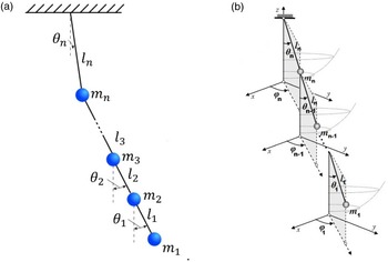
The total Hamiltonian of the system shown in Fig. 1(a) is computed via the Legendre transformation as follows:
 \begin{align} H=\sum _{j=1}^{n}p_{j}\dot{q}_{j} - L(\dot{q}_{j},\ldots,\dot{q}_{1},q_{j}, \ldots, q_{1}). \end{align}
(a)
 $n$
-DOF planar pendulum. (b)
 $n$
-DOF spherical pendulum.

For the Bang–Bang control, one requires to compute
 $n$
Hamiltonians and
 $n$
control signals
 $u_{j}$
for each DOF of the system. The
 $n$
Hamiltonians are computed as follows:
 \begin{align} H_{n}=\left (\sum _{j=1}^{n}p_{j}\dot{q}_{j} - L(\dot{q}_{j},\ldots,\dot{q}_{1},q_{j}, \ldots, q_{1})\right )-\left ( \sum _{j=1}^{n-1}p_{j}\dot{q}_{j} - L(\dot{q}_{j},\ldots,\dot{q}_{1},q_{j}, \ldots, q_{1})\right ), \end{align}
 \begin{align} H_{n-1}=\left (\sum _{j=1}^{n-1}p_{j}\dot{q}_{j} - L(\dot{q}_{j},\ldots,\dot{q}_{1},q_{j}, \ldots, q_{1})\right )-\left ( \sum _{j=1}^{n-2}p_{j}\dot{q}_{j} - L(\dot{q}_{j},\ldots,\dot{q}_{1},q_{j}, \ldots, q_{1})\right ), \end{align}
 \begin{align*} \vdots \end{align*}
 \begin{align} H_{2}=\left (\sum _{j=1}^{2}p_{j}\dot{q}_{j} - L(\dot{q}_{2},\dot{q}_{1},q_{2},q_{1})\right )-\left ( p_{1}\dot{q}_{1} - L(\dot{q}_{1},q_{1})\right ), \end{align}
 \begin{align} H_{1}=p_{1}\dot{q}_{1} - L(\dot{q}_{1},q_{1}). \end{align}
The sum of the Hamiltonians
 $H_j$
gives the total Hamiltonian of the system.
 \begin{align} H=\sum _{j=1}^{n}H_{j}. \end{align}
The recursive Hamiltonians should fulfill the condition
 $H_{j}(0)=0$
. The Hamiltonians are functions of the control
 $u_{j}$
for each DOF
 $H_{j}(p_{j},q_{j},u_{j})$
. The computed Hamiltonian depends on the control signal
 $u_{j}$
and then applying the maximum Pontryagin principle one gets two Hamiltonians a maximum and a minimum. Thus, one obtains 2
 $n$
Hamiltonian,
 $n$
are maximums and
 $n$
are minimums.
 \begin{align} H_{j}(p_{j},q_{j},u_{j})=H_{j}-B_{j}u_{j}. \end{align}
For the Bang–Bang control, all the control signals are
 \begin{align} u_{j}= \quad if \quad H(e)_{j_{max}}\gt H(e)_{j_{min}}\,\,\,\texttt{then}\,\,\, \quad -1 \quad else \quad 1, \end{align}
where
 $q_{j_{ref}}$
is the reference for the control related to each DOF
 $q_{j}$
, and the error
 $e=q_{j}-q_{j_{ref}}$
.
On can use the Newton–Euler recursive method of Subsection 5.1 to easily compute the Hamiltonians
 $H_j$
at each joint of any DOF robot manipulator
 \begin{align} H(\theta _i,\boldsymbol{p}_i)_i= \boldsymbol{p}_i\cdot \boldsymbol{s}_i- L(\theta _i, \dot{\theta }_i). \end{align}
This method can be applied for the case of
 $n$
-D spherical pendulums shown in Fig. 1(b), which have in each joint 2 DOF. Since each joint has 2 DOF, each Hamiltonian
 $H_j$
is related with two angles
 $\phi _{j}$
and
 $\theta _{j}$
, thus one split the Hamiltonian
 $H_j$
in the other two Hamiltonians.
 \begin{align} H_{j}=H_{\phi _{j}}+H_{\theta _{j}}. \end{align}
In total, one gets for the system
 $2n$
Hamiltonians.
7. Experimental analysis
In this section, we study the application of localized controllers derived using the local Hamiltonian Eq. (59) and local derivative momenta Eq. (62) for robot systems. The used localized controllers are the PD, slide modes, and Bang–Bang controllers. Since this work focuses on the control of spherical or serial robot manipulators, we cover the most important structures of robot arms. For the comparison, we used three well-known controllers, this is enough to validate the modeling and control using the motor algebra framework.
7.1. Bang–Bang control for a 2 DOF robot manipulator
Using the Newton–Euler iterative algorithm, we can compute the tensors of the Euler–Lagrange state equation with control signals as follows:
 \begin{align} M\left [\begin{array}{c} \ddot{\theta }_1\cr \\[5pt] \ddot{\theta }_2\end{array}\right ] +C\left (\left [\begin{array}{c} \dot{\theta }_1\cr \\[5pt] \dot{\theta }_2\end{array}\right ],\left [\begin{array}{c}{\theta }_1\cr \\[5pt]{\theta }_2\end{array}\right ]\right )+G\left (\theta _1,\theta _2\right )=\left [\begin{array}{c} b_1u_1\cr \\[5pt] b_2u_2\end{array}\right ], \end{align}
where
 \begin{align*} &M=\left [ \begin{array}{c@{\quad}c} (m_1+m_2)l_1^2 & m_2l_1l_2\cos (\theta _1-\theta _2)\cr \\[5pt] m_2l_1l_2\cos (\theta _1-\theta _2)& m_2l_2 \cr \\[5pt] \end{array}\right ] \\[5pt] &C\left (\left [\begin{array}{c} \ddot{\theta }_2\cr \\[5pt] \ddot{\theta }_1\end{array}\right ],\left [\begin{array}{c} \dot{\theta }_2\cr \\[5pt] \dot{\theta }_1\end{array}\right ] \right )=\left [\begin{array}{c@{\quad}c} 0 & m_2l_1l_2\dot{\theta }_2\sin (\theta _1-\theta _2)\cr \\[5pt] -m_2l_1l_2\dot{\theta }_1\sin (\theta _1-\theta _2)& 0 \end{array}\right ] \\[5pt] &G\left (\left [\begin{array}{c}{\theta }_2\cr \\[5pt]{\theta }_1\end{array}\right ]\right )=\left [\begin{array}{c} (m_1+m_2)gl_1\sin{\theta }_1\cr \\[5pt] m_2gl_2\sin{\theta }_2\end{array}\right ]. \end{align*}
Furthermore, using the Newton–Euler iterative algorithm of subsection (5.1), we can compute inward for each joint the following local Hamiltonians using generalized coordinates:
 \begin{align} H_2 = \frac{1}{2}m_2l_2^2\dot{\theta }_2^2-m_2gl_2\cos (\theta _2),\qquad\qquad\qquad\qquad\qquad\qquad\qquad\qquad \end{align}
 \begin{align} H_1 = \frac{1}{2}(m_1+m_2)l_1^2\dot{\theta }_1^2+m_2l_1l_2\dot{\theta }_1\dot{\theta }_2\cos (\theta _1-\theta _2)-(m_1+m2)gl_1\cos (\theta _1).\end{align}
Since the
 $H_1(0)=0$
and
 $H_2(0)=0$
, Eq. (76) becomes
 \begin{align} H_2(\theta _2)=\frac{1}{2}m_2l_2^2\dot{\theta }_2^2+m_2gl_2(1-\cos (\theta _2)),\qquad\qquad \end{align}
 \begin{align} \;H_1(\theta _1)&=\frac{1}{2}(m_1+m_2)l_1^2\dot{\theta }_1^2+m_2l_1l_2\dot{\theta }_1\dot{\theta }_2\cos (\theta _1-\theta _2)\nonumber \\[5pt] &\,\,\,\,+(m_1+m_2)gl_1(1-\cos (\theta _1)). \end{align}
A control algorithm that checks for the process variable exceeding or falling below the set point is called on/off control. This kind of control is also known as Bang–Bang control because the manipulated variable output of the controller rapidly changes between fully on and fully off involving no intermediate state. It has been shown that Bang–Bang control usually provides imprecise control of the process variable. In this work, we applied control only to revoluted joints. A rotation unit is geometrically speaking a dual of a prismatic joint because for the modeling of its rotation one uses rotors for revoluted joints and translators for the prismatic joints, thus it is possible to apply Bang–Bang control to prismatic joints.
In this work, Bang–Bang control is applied in a localized manner at each joint using the local Hamiltonians similar to in the state Eq. (75). These control signals
 $u_i=\pm 1, i=1,2$
switch between the scalar functions of
 $H_1$
and
 $H_2$
.
 \begin{align} H_2(\theta _2) = \frac{1}{2}m_2l_2^2\dot{\theta }_2^2+m_2gl_2(1-\cos (\theta _2))-b_2\theta _2u_2,\quad \end{align}
 \begin{align} H_1(\theta _1) &= \frac{1}{2}(m_1+m_2)l_1^2\dot{\theta }_1^2+m_2l_1l_2\dot{\theta }_1\dot{\theta }_2b\cos (\theta _1-\theta _2) \\[5pt] & \quad +(m_1+m_2)gl_1(1-\cos (\theta _1))-b_1\theta _1u_1\nonumber, \end{align}
Applying in Eqs. (80-82) the maximal principle of Pontryagin and setting the angle references
 $\theta _{1_{ref}}=20^o$
and
 $\theta _{2_{ref}}=30^o$
and
 $u_i=\pm 1, i=1,2$
for the switching in the Hamiltonians so that the Hamiltonians reach the zero value, we obtain the following equations:
 \begin{align} H_{11}&=\frac{1}{2}(m_1+m_2)l_1^2\dot{\theta }_1^2+m_2l_1l_2\dot{\theta }_1\dot{\theta }_2\cos \left ((\theta _1-\theta _{1_{ref}})-(\theta _2-\theta _{2_{ref}})\right )\nonumber \\[5pt] &\,\,\,\,+(m_1+m_2)gl_1(1-\cos (\theta _1-\theta _{1_{ref}}))-b_1(\theta _1-\theta _{1_{ref}}), \end{align}
 \begin{align} H_{12}&=\frac{1}{2}(m_1+m_2)l_1^2\dot{\theta }_1^2+m_2l_1l_2\dot{\theta }_1\dot{\theta }_2\cos \left ((\theta _1-\theta _{1_{ref}})-(\theta _2-\theta _{2_{ref}})\right ) \nonumber \\[5pt] &\,\,\,\,+(m_1+m_2)gl_1(1-\cos (\theta _1-\theta _{1_{ref}}))+b_1(\theta _1-\theta _{1_{ref}}), \end{align}
where
 $u_1=$
if
 $H_{12}\gt H_{11}$
then -1 else 1 and
 \begin{align} H_{21}=\frac{1}{2}m_2l_2^2\dot{\theta }_2^2+m_2gl_2(1-\cos (\theta _2-\theta _{2_{ref}}))-b_2(\theta _2-\theta _{2_{ref}}), \end{align}
 \begin{align} H_{22}=\frac{1}{2}m_2l_2^2\dot{\theta }_2^2+m_2gl_2(1-\cos (\theta _2-\theta _{2_{ref}}))+b_2(\theta _2-\theta _{2_{ref}}), \end{align}
where
 $u_2=$
if
 $H_{22}\gt H_{21}$
then -1 else 1. The control signals
 $u_i=\pm 1, i=1,2$
switch between the Hamiltonians
 $H_1$
and
 $H_2$
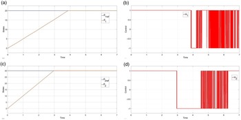
surfaces. Figure 3 shows the control signals and the error figures to reach a reference point. Note that even though that the controllers reach the references, they keep switching very rapidly between
 $\pm$
1.
2 DOF planar robot.

Hamiltonian Bang–Bang controller: (a) state
 $\theta _1$
: (b) control
 $u_1$
; (c) state
 $\theta _2$
: (d) control
 $u_2$
.

7.2. PD and sliding mode controller for a 2 DOF robot manipulator
Before constructing the law of control, it is necessary to compute Hamilton’s equations in the screw theory framework. The Hamiltonian on the phase space can be computed using Eqs. (25, 27) as follows:
 \begin{equation} \mathcal{H}\left (\theta,p,t\right )=\sum _{j=1}^n \frac{1}{2}\boldsymbol{P}_j^TN^{-1}_j\boldsymbol{P}_j+\widetilde{g}^T \widetilde{c}_j, \end{equation}
 \begin{equation} \frac{\partial \mathcal{H}\left ( \theta,p,t\right )}{\partial p_i} =\frac{1}{\boldsymbol{S}_i^TN_i\boldsymbol{S}_i}\left (p_i-\sum _{j=i+1}^n\boldsymbol{S}_i^T\boldsymbol{P}_j-\sum _{k=1}^{i-1}\boldsymbol{S}_i^T\boldsymbol{P}_{i,k} \right ), \end{equation}
 \begin{equation} \frac{\partial \mathcal{H}\left ( \theta,p,t\right )}{\partial \theta _i} = \sum _{j=i}^{n}\boldsymbol{P}_j^T\left [\boldsymbol{S}_i,N^{-1}_i\boldsymbol{P}_i\right ]-G^T_j\boldsymbol{S}_i, \end{equation}
where
 $\boldsymbol{S}_i$
is the twist
 $\boldsymbol{s}_i$
written as a 6
 $\times$
1 vector and the momentum
 ${{\textbf{P}}}_i$
is a 6
 $\times$
1 vector as well.
According to Eq. (63), the derivative of the momenta at
 $i$
-joint is
 \begin{equation} \dot{p}_i =\tau _i + \sum _{j=i}^{n} G^T_j\boldsymbol{S}_i-\boldsymbol{P}_j^T\left [\boldsymbol{S}_i,N^{-1}_i\boldsymbol{P}_i\right ]. \end{equation}
A serial robotic system will track a desired smooth function applying the following decentralized PD law of control:
 \begin{equation} \begin{split} \tau _i={K_p}_i\widetilde{\theta }_i+{K_v}_i\widetilde{p}_i+\dot{{p_d}}_i- \sum _{j=i}^n\boldsymbol{P}_j^T\left [N_i^{-1}\boldsymbol{P}_i,\boldsymbol{S}_i\right ]-G^T_j\boldsymbol{S}_i \end{split}, \end{equation}
where
 $\widetilde{p}_i={p_d}_i-p_i$
is the error between the desired momentum and the measured momentum and
 $\widetilde{\theta }_i={\theta _d}_i-\theta _i$
is the error between the desired joint position and the measured joint position and
 ${K_p}_i,{K_v}_i \in \mathbb{R}^+$
.
A robotic system will reach the home position by applying the following decentralized sliding modes law of control:
 \begin{equation} \tau _i=K_isign(\mathcal{S}_i)+{K_{\mathcal{S}}}_i{\mathcal{S}}_i+\widetilde{\theta }_i - \sum _{j=i}^n\boldsymbol{S}_j^T\{\boldsymbol{S}_i,N_j{ L}_i\}-G_j\cdot L_i, \end{equation}
where
 $\{\boldsymbol{S}_i,N_j{ L}_i\}=N_j\left [\boldsymbol{S}_i,{ L}_i\right ]$
and in each joint,
 $\mathcal{S}_i=-\sum _{j=i}^{n}{ L}_i^T N_j\boldsymbol{S}_j+\widetilde{\theta }_i$
is the sliding surface and
 $K_i,{K_{\mathcal{S}}}_i \in \mathbb{R}^+$
.
Consider the two-link manipulator with revolute joints illustrated in Fig. 2. In addition, the manipulator link lengths are
 $l_1$
and
 $l_2$
, and the link masses are
 $m_1$
and
 $m_2$
, where these masses are concentrated at the end of each link.
The dynamic of the proposed robot is computed using (55). Hence, the dynamic of each joint can be written as the following:
 \begin{align} \tau _1 = \dot{V}_1^T N_1L_1+V_1^TN_1\left [L_1,V_1\right ]-G_1\cdot L_1+\dot{V}_2^TN_2L_1+V_2^TN_2\left [L_1,V_2\right ]-G_2\cdot L_1, \end{align}
 \begin{align} \tau _2 = \dot{V}_2^T N_2L_2+V_2^T N_2\left [L_2,V_2\right ]-G_2\cdot L_2.\end{align}
Considering
 $V_1=L_1 \dot{\theta }_1$
and
 $V_2=L_1 \dot{\theta }_1+L_2 \dot{\theta }_2$
. Thus, the accelerations are constructed by
 \begin{align} \dot{V}_1 = \frac{d}{dt}\left (L_1 \dot{\theta }_1 \right )=L_1\ddot{\theta }_1, \end{align}
 \begin{align} \dot{V}_2 = \frac{d}{dt}\left (L_1 \dot{\theta }_1+L_2 \dot{\theta }_2 \right )=L_1\ddot{\theta }_1+L_2\ddot{\theta }_2+ad(V_1)L_2\dot{\theta }_2=L_1\ddot{\theta }_1+L_2\ddot{\theta }_2+\left [L_1,L_2\right ]\dot{\theta }_1\dot{\theta }_2. \end{align}
Taking the previous accelerations
 $(\dot{V}_1,\dot{V}_2)$
and velocities
 $(V_1, V_2)$
into (92) and (93), the dynamic of the robot can be written as follows:
 \begin{align} \tau _1&= L_1^T N_1L_1\ddot{\theta }_1+L_1^TN_2L_1\ddot{\theta }_1+L_1^TN_2L_2\ddot{\theta }_2 +2L_1^TN_2\left [L_1,L_2\right ]\dot{\theta }_1\dot{\theta }_2 \nonumber \\[5pt] &\quad +L_2^TN_2\left [L_1,L_2\right ]\dot{\theta }_2^2-G_1^TL_1-G_2^TL_1, \end{align}
 \begin{align} \tau _2 = L_1^T N_2L_2\ddot{\theta }_1+L_2^T N_2L_2\ddot{\theta }_2-L_1^T N_2\left [L_1,L_2\right ]\dot{\theta }_1^2-G_2^TL_2. \end{align}
7.2.1. PD controller
Given the state variables
 $x_1,x_2 \in \mathbb{R}^2$
, where
 $x_1=\left (\theta _1,\theta _2\right )^T$
and
 $x_2=\left ( \dot{\theta }_1,\dot{\theta }_2 \right )^T$
, the closed-loop system can be represented using Eq. (90) as follows:
 \begin{equation} \small \left [ \begin{array}{cccc} \dot{x_1} \\[5pt] \dot{x_2} \\[5pt] \end{array} \right ] = \left [ \begin{array}{cccc} x_2 \\[5pt] -\begin{pmatrix} L_1^TN_1L_1+L_1^TN_2L_1 & L_1^TN_2L_2 \\[5pt] L_1^TN_2L_2 & L_2^TN_2L_2 \end{pmatrix}^{-1}\left [ \begin{pmatrix}{K_p}_1 & 0\\[5pt] 0 &{K_p}_2 \end{pmatrix}x_1 +\begin{pmatrix}{K_v}_1 & 0\\[5pt] 0 &{K_v}_2 \end{pmatrix}x_2 -B(\dot{\theta }_1,\dot{\theta }_2] \right ] \end{array} \right ] \end{equation}
where
 \begin{equation} B(\dot{\theta }_1,\dot{\theta }_2)= \left [ \begin{array}{cccc} 2L_1^TN_2\left [L_1,L_2\right ]\dot{\theta }_1\dot{\theta }_2 +L_2^TN_2\left [L_1,L_2\right ]\dot{\theta }_2^2\\[5pt] -L_1^T N_2\left [L_1,L_2\right ]\dot{\theta }_1^2 \\[5pt] \end{array} \right ] \end{equation}
To simulate the results of the example, it is necessary to implement the parameters in Table I with
 ${K_p}_1,{K_p}_2=150$
and
 ${K_v}_1,{K_v}_2=50$
. The simulations were conducted using the Euler integration method, with a step size of
 $0.001 s$
. The initial conditions were selected as
 $x_1(0)=x_2(0)=0$
and the desired values as
 ${\theta _d}_1=20^{\circ },{\theta _d}_2=30^{\circ }$
. Hence, the results of the example are presented in Fig. 4.
PD controller: (a) states: angles
 $x_1$
and angular velocities
 $x_2$
. (b) Robot motion.

7.2.2. Sliding mode controller
Suppose
 $x_1,x_2 \in \mathbb{R}^2$
, where
 $x_1=\left (\theta _1,\theta _2\right )^T$
and
 $x_2=\left ( \dot{{\theta }}_1,\dot{{\theta }}_2 \right )^T$
. Then, the closed-loop system using Eq. (91) can be represented by
 \begin{equation} \begin{split} \left [ \begin{array}{cccc} \dot{x_1} \\[5pt] \dot{x_2} \\[5pt] \end{array} \right ] = \left [ \begin{array}{cccc} x_2 \\[5pt] \begin{pmatrix} L_1^TN_1L_1+L_1^TN_2L_1 & L_1^TN_2L_2 \\[5pt] L_1^TN_2L_2 & L_2^TN_2L_2 \end{pmatrix}^{-1}\left [ \begin{pmatrix} -K_1sign\left [\mathcal{S}_1\right ]-{K_{\mathcal{S}}}_1 \\[5pt] -K_2sign\left (\mathcal{S}_2\right )-{K_{\mathcal{S}}}_2 \end{pmatrix}-x_2 -B(x_2) \right ] \\[5pt] \end{array} \right ] \end{split} \end{equation}
where
 \begin{align} \mathcal{S}_1&=L_1^TN_1L_1\dot{\theta _1}+L_1^TN_2L_1\dot{\theta _1}+L_1^TN_2L_2\dot{\theta _2}+\theta _1\nonumber \\[5pt] \mathcal{S}_2&= L_1^TN_1L_2\dot{\theta _1}+L_2^TN_2L_2\dot{\theta _2}+\theta _2\nonumber \\[5pt] B(x_2)&= \left [ \begin{array}{cccc} 2L_1^TN_2\left [L_1,L_2\right ]\dot{\theta }_1\dot{\theta }_2 +L_2^TN_2\left [L_1,L_2\right ]\dot{\theta }_2^2\\[5pt] L_2^TN_2\left [L_1,L_2\right ]\dot{\theta }_1\dot{\theta }_2 \\[5pt] \end{array} \right ] \end{align}
To simulate the results of the example, it is necessary to implement the parameters in Table I with
 $K_1,{K}_2 = 1$
and
 ${K_{\mathcal{S}}}_1,{K_{\mathcal{S}}}_2 =50$
. The simulations were conducted using the Euler integration method, with a step size of
 $0.001 s$
. The initial conditions were selected as
 $x_1(0)=[45^{\circ },10^{\circ }]^T$
and
 $ x_2(0)=[0,0]^T$
. Using the sliding mode controller [Reference Utkin, Guldner and Shi28], we carry out a tracking experiment. Moreover, it is necessary to take care with the adjustable gains because a small variable cannot easily converge to the position for the case of different robots. Therefore, it is important to adjust the gain depending on the application.
Parameters of the robot.

Figure 5(a) and (b) presents the evolution of the angles and angular velocities of the two joints during the tracking. These experiments show that our sliding mode controller performs very well in both stability and tracking. Figure5(c) and (d) shows how well the sliding mode controller manages the 2 DOF robot arm to follow a nonlinear curve.
Sliding modes controller: (a) states: angles
 $x_1$
; (b) angular velocities
 $x_2$
; (c) sliding modes surfaces; and (d) robot motion.

7.3. Bang–Bang control for a 4 DOF double spherical pendulum
The Lagrangian associated with the double spherical pendulum is given by
 \begin{align} L=T-V, \end{align}
where
 \begin{align} T&= \frac{1}{2}\left (m_{1}+m_{2} \right ) l_{2}^{2}\left (\dot{\theta _2}^{2} +\sin ^2\theta _{2} \dot{\phi _2}^2 \right ) +\frac{1}{2}m_{1}l_{1}^{2}\left (\dot{\theta _1}^{2} +\sin ^2\theta _{1} \dot{\phi _1}^2 \right )\nonumber \\[5pt] &\quad + m_{1}l_{1}l_{2}\dot{\theta }_{1}\dot{\theta }_{2}\sin \theta _{1} \sin \theta _{2} +m_{1}l_{1}l_{2}\cos \left (\phi _{2}-\phi _{1} \right )\left ( \cos \theta _{1}\cos \theta _{2}\dot{\theta _1} \dot{\theta _2} + \sin \phi _{1} \sin \phi _{2} \dot{\phi _1} \dot{\phi _2} \right ) \nonumber \\[5pt] &\quad +m_{1}l_{1}l_{2}\sin \left (\phi _{2}-\phi _{1} \right )\left ( \cos \theta _{2}\sin \theta _{1}\dot{\phi _1} \dot{\phi _2} - \sin \theta _{2} \cos \theta _{1} \dot{\phi _2} \dot{\theta _1} \right ), \end{align}
 \begin{align} V = -\left (m_{1}+m_{2} \right )gl_{2}\cos \theta _{2}- m_{1}gl_{1}\cos \theta _{1}. \end{align}
The motion equations can be obtained from the Lagrangian of the double spherical pendulum
 \begin{align} M(\theta _{j},\phi _{j})\left ( \begin{array}{ccc} \ddot{\theta _{j}} \\[5pt] \ddot{\phi _{j}} \end{array} \right ) +C(\theta _{j},\dot{\theta _{j}},\phi _{j},\dot{\phi _{j}})\left ( \begin{array}{ccc} \dot{\theta _{j}} \\[5pt] \dot{\phi _{j}} \end{array} \right ) +G(\theta _{j},\phi _{j})=Bu. \end{align}
As we showed in the previous example of the double pendulum by applying the V.M. Yepez theorem, it is extremely difficult to compute the Hamiltonian for manipulators of more than 2 DOF. This shows that it is better to compute the Hamiltonian of the system via the Legendre transformation and in a local manner apply the V.M. Yepez theorem.
 \begin{align} H(q_{j},p_{j},t)=\sum p_{j}\dot{q_{j}}-L(q_{j},\dot{q_j},t). \end{align}
For the double spherical pendulum, the Hamiltonian of the system is given by
 \begin{align} H=T+V. \end{align}
Based on the Hamiltonian of the 4 DOF of the system, we can derive four Hamiltonians for each DOF which are obtained using the Newton–Euler recursive algorithm explained in Subsection 5.1, so the computed Hamiltonian
 $H_j$
at the j-join is
 \begin{align} H_{j}(\theta _j, \phi _j,\boldsymbol{p}_j)= \boldsymbol{p}_j\cdot \boldsymbol{s}_j- L(\theta _j, \phi _j,\dot{\theta }_j, \dot{\phi }_j). \end{align}
The computed four Hamiltonians are
 \begin{align} H_4 & = \frac{1}{2}\left (m_{1}+m_{2} \right ) l_{2}^{2}\dot{\theta _2}^{2} +m_{1}l_{1}l_{2}\dot{\theta }_{1}\dot{\theta }_{2}\sin \theta _{1} \sin \theta _{2},\\[5pt] &\quad + m_{1}l_{1}l_{2}\cos \left (\phi _{2}-\phi _{1} \right )\left ( \cos \theta _{1}\cos \theta _{2}\dot{\theta _1} \dot{\theta _2} + \sin \phi _{1} \sin \phi _{2} \dot{\phi _1} \dot{\phi _2} \right ) \nonumber \\[5pt] &\quad + m_{1}l_{1}l_{2}\sin \left (\phi _{2}-\phi _{1} \right )\left ( \cos \theta _{2}\sin \theta _{1}\dot{\phi _1} \dot{\phi _2} - \sin \theta _{2} \cos \theta _{1} \dot{\phi _2} \dot{\theta _1} \right )-\left (m_{1}+m_{2} \right )gl_{2}\cos \theta _{2} \nonumber \end{align}
 \begin{align} H_3 =\frac{1}{2}\left (m_{1}+m_{2} \right ) l_{2}^{2}\left ( \sin ^2\theta _{2} \dot{\phi _2}^2 \right ), \end{align}
 \begin{align} H_2 = \frac{1}{2}m_{1}l_{1}^{2}\dot{\theta _1}^{2}-m_{1}gl_{1}\cos \theta _{1}, \end{align}
 \begin{align} H_1 = \frac{1}{2}m_{1}l_{1}^{2}\left (\sin ^2\theta _{1} \dot{\phi _1}^2 \right ). \end{align}
One applies the maximum principle of Pontryagin to
 $H_{1}$
,
 $H_{2}$
,
 $H_{3}$
y
 $H_{4}$
to obtain two Hamiltonians a maximum and a minimum for each function, resulting then in eight Hamiltonians, where one has to impose the condition
 $H_{j}(0)=0$
. The motion equations are obtained from the system Hamiltonians of the double spherical pendulum including the Bang–Bang control.
 \begin{align} \frac{d}{dt}\left ( \frac{\partial L}{\partial \dot{\theta _{1}}}\right )- \frac{\partial L}{\partial \theta _{1}} = b_{1}u_{1}, \end{align}
 \begin{align} \frac{d}{dt}\left ( \frac{\partial L}{\partial \dot{\theta _{2}}}\right )- \frac{\partial L}{\partial \theta _{2}} = b_{2}u_{2}, \end{align}
 \begin{align} \frac{d}{dt}\left ( \frac{\partial L}{\partial \dot{\phi _{1}}}\right )- \frac{\partial L}{\partial \phi _{1}} = b_{3}u_{3}, \end{align}
 \begin{align} \frac{d}{dt}\left ( \frac{\partial L}{\partial \dot{\phi _{2}}}\right )- \frac{\partial L}{\partial \phi _{2}} = b_{4}u_{4}. \end{align}
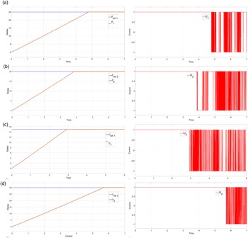
Figure 7 shows the control signals and the error figures to reach a reference point. Note that even though the controllers reach the references, they keep switching very rapidly between
 $\pm$
1.
4 DOF spherical pendulum.

(a) Angle state
 $\theta _{1}$
and control
 $u_{1}$
. (b) Angle state
 $\theta _{2}$
and control
 $u_{2}$
. (c) Angle state
 $\phi _{1}$
and control
 $u_{3}$
. (d) Angle state
 $\phi _{2}$
and control
 $u_{4}$
.

7.4. Sliding mode controller for a 4 DOF double spherical pendulum
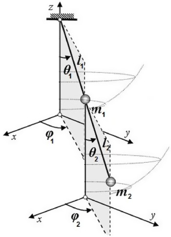
Consider the two-link manipulator with four revolute joints as illustrated in Fig. 6. The manipulator link lengths are
 $l_1$
and
 $l_2$
, and the link masses are
 $m_1$
and
 $m_2$
, where these masses are concentrated at the end of each link.
The Newton–Euler iterative algorithm is based on Eq. (55), accordingly the resulting wrench at each is given by
 \begin{align} \tau _i= \sum _{j=i}^{5} \left [\texttt{N}_j(\dot{{\textbf{s}}}_j-{{\textbf{G}}})\cdot{{\textbf{L}}}_i+{\{{{\textbf{s}}}_j,\texttt{N}_j{{\textbf{s}}}_j \}}\cdot{{\textbf{L}}}_i \right ]. \end{align}
To formulate the sliding-mode-based control, first, we require to represent in state variables the dynamics of the robot arm. This procedure is an extension as presented for the 2 DOF robot arm of Subsection 7.2. We use Eq. (55) and extend Eqs. (100)–(101) of the 2 DOF manipulator to the 4 DOF double spherical pendulum. To simplify the equation, we gather all the terms in matrices as follows:
 \begin{equation} M(x)\ddot{x} + C(\dot{x},x)\dot{x} + G(x) = \tau, \end{equation}
where
 $M$
is the inertia matrix,
 $C$
is the Coriolis and centripetal matrix,
 $G(x)$
is the gravity vector,
 $\tau$
is the actuating torque vector,
 $x$
is the vector state corresponding with the angular displacement of each joint, and
 $\dot{x}$
and
 $\ddot{x}$
are the first and second derivatives of the state vector corresponding to the velocity and acceleration, respectively. The relation between the Hamiltonian and the Euler–Lagrange equations can be established by using the Legendre’s transformation as mentioned in Subsection 4.
Using the previous Eq. (118), the space state model for the angular displacements and their velocities of the joints is defined as follows:
 \begin{align} \dot{x}_1 = x_2, \end{align}
 \begin{align} \dot{x}_2 = f(x_1, x_2) + B(x_1, x_2)u, \end{align}
where
 $x_1 = [\phi _1, \theta _1, \phi _2, \theta _2]^\top$
and
 $x_2 =[\dot{\phi }_1, \dot{\theta }_1, \dot{\phi }_2, \dot{\theta }_2]^\top$
are the state variables (angular displacements and velocities, respectively),
 $f(x_1,x_2)= -M^{-1}(x_1) \left ( C(x_1,x_2)x_2 + G(x_1) \right )$
,
 $B(x_1,x_2) = M^{-1}(x_1)$
,
 $u = \tau$
the signal control laws.
Since the purpose of the controller is to track trajectories, if we define the tracking error as
 $e_1 = x_d-x_1$
and using (119-120), the error system is described as
 \begin{align} \dot{e}_1 & = \dot{x}_d - x_2 = e_2 \nonumber \\[5pt] \dot{e}_2 & = \ddot{x}_d - f(x_1, x_2) - B(x_1, x_2)u. \end{align}
Because the system can contain uncertainties attributed to parametric variations, unmodeled dynamics, and external disturbances, it is necessary to add a term that contains these uncertainties, so our error system is redefined as
 \begin{align} \dot{e}_1 & = e_2 \nonumber \\[5pt] \dot{e}_2 & = \ddot{x}_d - f(x_1, x_2) - B(x_1, x_2)u_0 - B(x_1, x_2)u_1 + h(x_1, x_2, t), \end{align}
where
 $h(x_1, x_2, t)$
satisfies the matching condition [Reference Utkin, Guldner and Shi28]. Besides,
 $h(x_1, x_2, t)$
must be bounded by known positive defined scalar functions such that
 \begin{equation*} \left \lVert h(x_1, x_2, t)\right \lVert \leq h_i^+(x_1, x_2, t), \, i=1, \ldots, n. \end{equation*}
Once the error system model of our robotic system is obtained, we proceed to design the law of control. The law of control is defined as
 \begin{equation} u = u_0 + u_1, \end{equation}
where
 $u_0$
is computed using the inverse dynamic algorithm [Reference Spong, Hutchinson and Vidyasagar29] for the nominal system and
 $u_1$
is an integral sliding mode control algorithm that deals with external disturbances and parametric variations.
First, we describe
 $u_0$
as follows:
 \begin{equation} u_0 = M(x_1) a_d + C(x_1,x_2)x_2 + G(x_1), \end{equation}
where
 $a_d$
is the desired dynamics that will be designed later.
Substituting the control law
 $u_0$
(124) in the second equation of the error system (122), we have the following:
 \begin{align} \dot{e}_2 & = \ddot{x}_d - f(x_1, x_2) + B(x_1, x_2)u_0 + h(x_1, x_2, t) \nonumber \\[5pt] & = \ddot{x}_d - M^{-1}(x_1) \left (C(x_1,x_2)x_2+G(x_1) \right ) + M^{-1}(x_1)u_0 + h(x_1, x_2, t) \nonumber \\[5pt] & = \ddot{x}_d - M^{-1}(x_1) \left (u_0 - C(x_1,x_2)x_2 - G(x_1) \right ) + h(x_1, x_2, t) \nonumber \\[5pt] & = \ddot{x}_d - a_d + h(x_1, x_2, t), \end{align}
which cancels the internal dynamics. To ensure the tracking of the references, we then define
 $ a_d$
as follows:
 \begin{align} a_d & = \ddot{x}_d - K_p \left (x_d - x_1\right ) - K_d \left (\dot{x}_d - x_2\right ) \nonumber \\[5pt] & = \ddot{x}_d - K_p e_1 - K_d e_2, \end{align}
where
 $x_d$
,
 $\dot{x}_d$
y
 $\ddot{x}_d$
are the position, velocity, and acceleration references, and
 $K_p$
y
 $K_d$
are
 $4 \times 4$
matrices. Then, the error system with
 $u_0$
is proposed as follows:
 \begin{align} \dot{e}_1 = e_2, \end{align}
 \begin{align} \dot{e}_2 = K_p e_1 + K_d e_2 + h(x_1, x_2, t).\end{align}
A simple way to design the gain matrices
 $K_p$
and
 $K_d$
is
 \begin{align} K_p & = \text{diag} \left ( \omega _1^2, \, \omega _2^2, \, \ldots, \, \omega _n^2 \right ) \\[5pt] K_d & = \text{diag} \left ( 2\omega _1, \, 2\omega _2, \, \ldots, \, 2\omega _n \right ), \nonumber \end{align}
which, leaving aside the term
 $h(x_1, x_2, t)$
, results in a decoupled closed-loop system, where each response of each joint is equal to the response of a critically damped second-order system with natural frequency
 $\omega _i$
, which determines the velocity response of the joints, or equivalently, the decay rate of the tracking error.
It is noteworthy that to compute
 $u_0$
, the inverse dynamics can be calculated using the Newton–Euler algorithm described in Section 5. To deal with the term
 $h(x_1, x_2, t)$
, which includes parametric variations and disturbances of the system, the control law
 $u_1$
is designed by using the integral sliding mode algorithm as mentioned above. This algorithm presupposes the existence of a previously designed controller for the nominal plant (without disturbances),
 $u_0$
, adding to this existing controller a discontinuous term to force the occurrence of sliding modes and thus obtaining a response as if the plant was the nominal system with its closed-loop controller, despite external disturbances and parametric variations of the system.
Sliding mode-based control: (a) control signals
 $U_1,U_2,U_3,U_4$
. (b) Space
 $x,y,z$
errors. (c) Motion in space
 $(x,y,z)$
. (d) State angle errors. (e–h) States angles
 $\phi _1,\phi _2,\theta _1,\theta _2$
-.

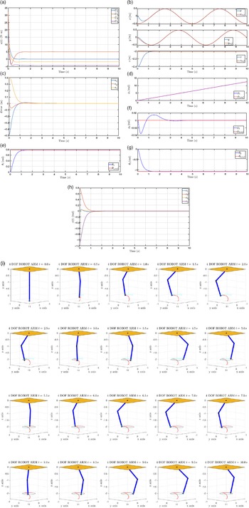
Sliding mode-based control: (a) control signals
 $U_i$
. (b) Space (x,y,z) tracking. (c) Space
 $x,y,z$
errors. (d–g) States angles
 $\phi _1, \phi _2, \theta _1, \theta _2$
. (h) Errors of state angle
 $\phi _1, \phi _2, \theta _1, \theta _2$
. (i) Sequence of tracking.

For
 $u_1$
, we define the sliding surface
 \begin{equation} s = \sigma (x) + z, \end{equation}
where
 $\sigma (x)=Ce_1+e_2$
and
 $z$
is the integral term that will be determined later. Then, if we derive (130) and substitute (122) and (123) in the result, we have
 \begin{equation} \dot{s} = Ce_2 + \ddot{x}_d - f(x_1, x_2) - B(x_1, x_2)u_0 - B(x_1, x_2)u_1 - h(x_1, x_2, t) + \dot{z}, \end{equation}
and defining
 \begin{equation} \dot{z} = Ce_2 + f(x_1, x_2) + B(x_1, x_2)u_0 - \ddot{x}_d, \, z(0) = -Ce_1(0)-e_2(0), \end{equation}
Eq. (131) reduces to
 \begin{equation} \dot{s} = - B(x_1, x_2)u_1 - h(x_1, x_2, t). \end{equation}
Now it is necessary to propose the control law
 $u_1$
, which will be designed using the super-twisting algorithm
 \begin{align} u_1 & = \alpha _1 \left \lvert{s}\right \rvert ^{1/2} \textrm{sign}\left ({s}\right ) + v \nonumber \\[5pt] \dot{v} & = \alpha _2 \textrm{sign}\left ({s}\right ). \end{align}
Substituting previous Eq. (134) in (133), the dynamics of the sliding surface is described as
 \begin{align} \dot{s} & = -B(x_1, x_2) ( \alpha _1 \left \lvert{s}\right \rvert ^{1/2} \textrm{sign}\left ({s}\right ) + v) + h(x_1, x_2, t), \end{align}
 \begin{align} \dot{v} = \alpha _2 \textrm{sign}\left ({s}\right ). \end{align}
It is possible to probe that the dynamics of the sliding surface is globally asymptotically stable [Reference Moreno and Osorio30] with certain conditions of gains
 $\alpha _1$
and
 $\alpha _2$
. With the explained control above, it will be achieved that the control
 $u_1$
rejects the disturbance
 $h(x_1, x_2, t)$
, that is,
 $B(x_1, x_2)u_1=-h(x_1,x_2,t)$
and even more, achieve the error system has the form
 \begin{align} \dot{e}_1 & = e_2 \nonumber \\[5pt] \dot{e}_2 & = \ddot{x}_d - f(x_1, x_2) - B(x_1, x_2)u_0, \end{align}
which is equivalent to the nominal system with control signal
 $u_0$
. It should be noted that
 $u_0$
was designed such that the nominal system tracks the desired references.
In order to show the performance of the proposed controller, two simulation experiments were developed. The parameters for the two-link manipulator are the same as described in the previous section. The values of the parameters of the controller used are as follows:
 $\alpha _1 = \textrm{diag}(3,3,1.5,1.8)$
,
 $\alpha _2 = \textrm{diag}(0.3,0.3,0.3,0.3)$
,
 $C = \textrm{diag}{1,1,1,1}$
,
 $K_p = \textrm{diag}(25,25,25,25)$
,
 $K_d = \textrm{diag}(10,10,10,10)$
.
For the first simulation experiment, the reference is described as
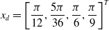 $x_d = \left[\dfrac{\pi }{12},\dfrac{5\pi }{36},\dfrac{\pi }{6},\dfrac{\pi }{9}\right]^T$
, which corresponds to fixed point in the space.
Figure 8 shows the double pendulum reaching a 3D point. It shows the control signals, the states, and angles evolution as their errors. Compared with the Bang–Bang control of the previous subsection, the integral sliding modes with super-twisting diminish chattering and reject matched perturbations.
Figure 9 shows the results for tracking a nonlinear trajectory. It shows the control signals, the states, and angles evolution as their errors. The integral sliding modes with super-twisting diminish chattering and reject matched perturbations.
8. Conclusion
In this work, the authors show the importance of the Hamiltonian in control theory. Instead of using the Lagrangian formulation of electromechanical or robotic systems, our work is focused on robot dynamics by its Hamiltonian. We compute the Hamiltonians, dynamics, and applied controllers using screw theory in the motor algebra. By using the recursive Newton–Euler dynamics, we can compute the Hamiltonians for each joint. Thanks to the screw theory, it is possible to compute recursively the Hamiltonian and the dynamics for each joint for robot manipulators of n DOF. As a result, we can apply local controllers to each joint.
In the experimental analysis, using simulations, we compute via the Newton–Euler dynamics and the Hamiltonians for a planar 2 DOF robot arm and a spherical pendulum of 4 DOF. We apply and compare four controllers: Bang–Bang., PD, basic sliding modes, and integral sliding modes together with super-twisting. We show that the sliding-mode-based controllers diminish chattering and reject matched perturbations. In future work, we will continue to relate geometric algebra and nonlinear control. We will develop observers ad new nonlinear controllers using the motor algebra framework and conformal geometric algebra.
Compliance with ethical standards
This study was funded by Mexican Conacyt Grant A1-S-1042.
Conflict of interest
The authors declare that they have no conflict of interest.
Authors participation
All authors have contributed in an equal manner to the elaboration of the article.