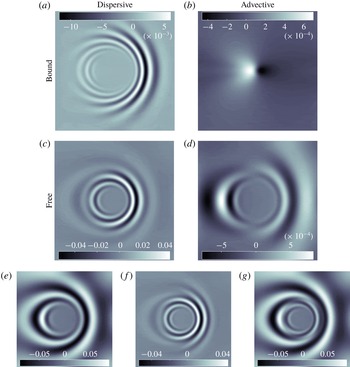
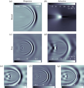
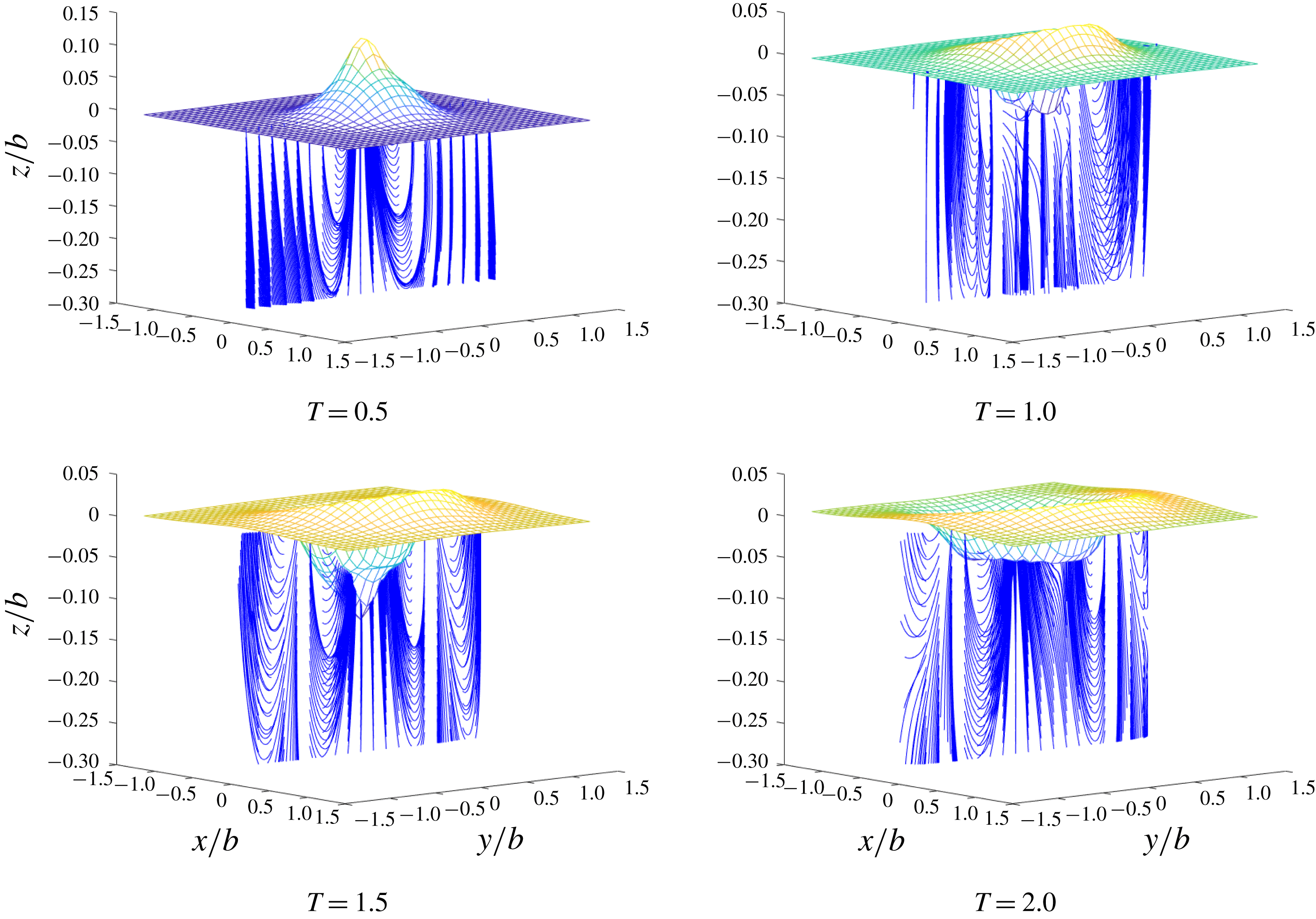
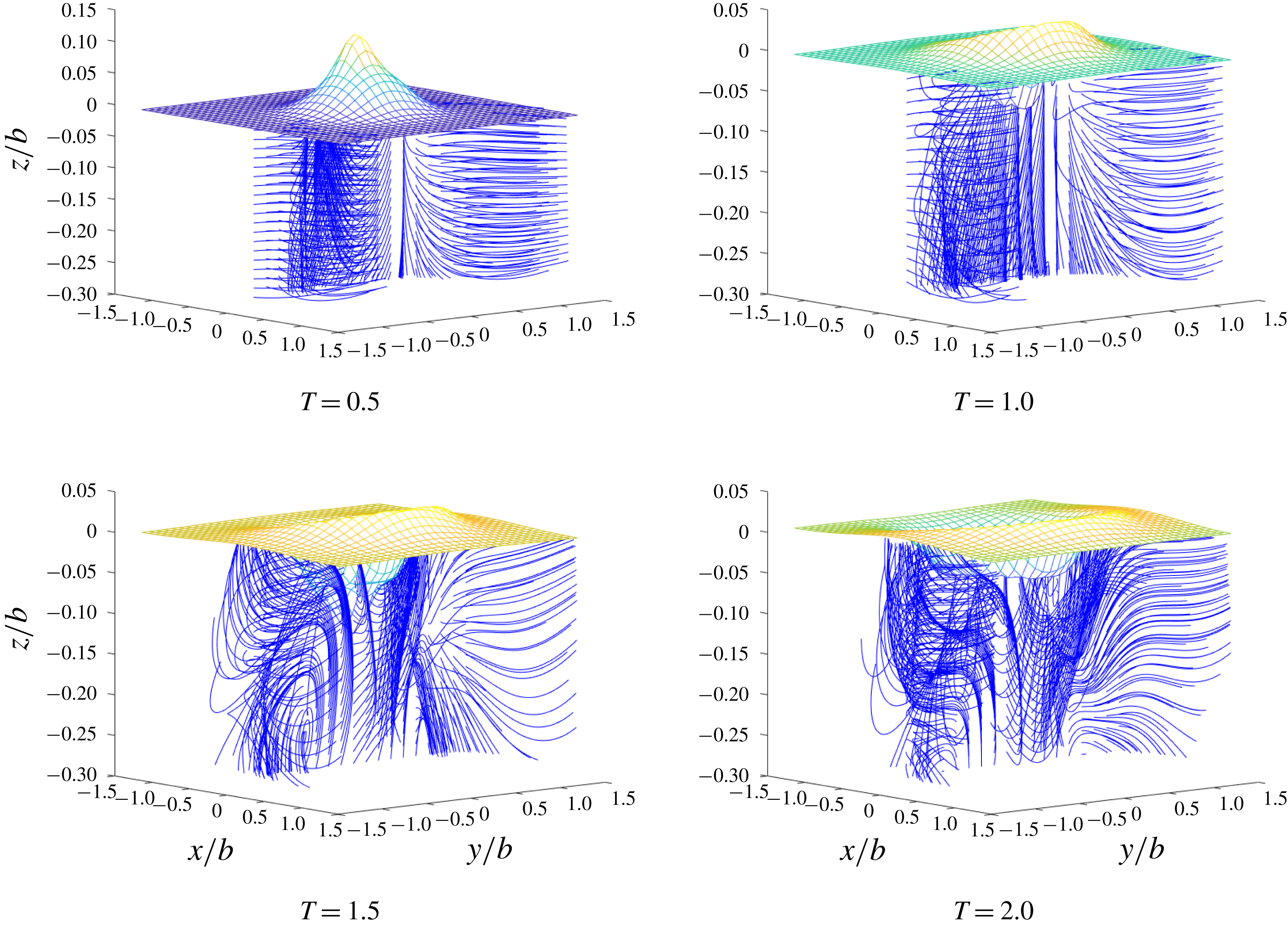
1 Introduction
Ring waves are a canonical wave pattern studied scientifically for two centuries pioneered by Cauchy (Reference Cauchy1816) and Poisson (Reference Poisson1818). Even in the simplest situation, however – deep water gravity waves – the effect of weakly nonlinear wave steepness on these patterns has not been previously studied, and we find herein that they are profound and non-trivial. The addition of a shear current, as recently studied to first order (Ellingsen Reference Ellingsen2014a ), makes the behaviour even richer.
Traditionally, the analysis of a deterministic field of waves have been separated into two categories – ray theory and mode coupling theory dealing with wave interactions in Fourier space (Wehausen & Laitone Reference Wehausen, Laitone and Flügge1960; Whitham Reference Whitham1974). This text is concerned with the latter category.
Within mode coupling theory an extensive family of methods exists for problems where the wave distribution is narrowly centred around some specific wave vector. Many of these narrow band approximation methods revolve around the application of multiple scale analysis. An example is the nonlinear Schrödinger equation, which can be obtained for the evolution of narrow banded wave packets (Stewartson & Stuart Reference Stewartson and Stuart1971). Developed from the same principle, but with a different approach, is the equation derived by Zakharov (Reference Zakharov1968) during the same period. A number of years later this equation gained broader recognition through a more extensive paper by Crawford et al. (Reference Crawford, Lake, Saffman and Yuen1981). Multiple scale analysis can also be applied in systems oriented about the dispersive wave packets to yield equations of Korteweg–de Vries (KdV) type. This type of method has been used to study the far field of ring waves (Johnson Reference Johnson1990; Khusnutdinova & Zhang Reference Khusnutdinova and Zhang2016a ,Reference Khusnutdinova and Zhang b ). Models such as those just mentioned have proven adept at predicting phenomena such as the formation of rogue waves (Kharif & Pelinovsky Reference Kharif and Pelinovsky2003) and are suitable for investigating wave packet stability in the presence of shear (Thomas, Kharif & Manna Reference Thomas, Kharif and Manna2012; Francius & Kharif Reference Francius and Kharif2017). The fundamental reason for the diverse wave phenomena occurring in the presence of vorticity is the change in dispersion properties due to the interaction between waves and current; see e.g. Ellingsen (Reference Ellingsen2014a ) and the classic review by Peregrine (Reference Peregrine1976).
The present paper revolves around mode coupling techniques for weakly nonlinear boundary value problems. A formalism is used similar to that presented by Phillips (Reference Phillips1960) and Longuet-Higgins & Phillips (Reference Longuet-Higgins and Phillips1962a ) for selective wave components, and by Hasselmann (Reference Hasselmann1962, Reference Hasselmann1963), Benney (Reference Benney1962) and Holliday (Reference Holliday1977) for spectra. Resonance and energy transfer between modes are the main foci in these references.
With the inclusion of a shear field new mechanisms for instability arise. Notable situations of wave–shear resonance include boundary layer transitions (Benney & Lin Reference Benney and Lin1960; Benney Reference Benney1961, Reference Benney1964) and wind-driven mixing phenomena in the upper ocean layer (Craik Reference Craik1970; Craik & Leibovich Reference Craik and Leibovich1976). Other interesting resonance effects involve resonant triads in the presence of strongly sheared flows, possible because the shear distorts the otherwise monotonic shape of the dispersion curve (Craik Reference Craik1968). The viscous regions of critical layers appear to be a vital mechanism for energy transfer in this case. Interactions between surface and ‘vorticity waves’ in stratified flows is another notable example of resonance (Drivas & Wunsch Reference Drivas and Wunsch2016). Much useful insight into mode interaction phenomena in surface waves is gathered in the monographs by West (Reference West1981) and Craik (Reference Craik1986). Recent studies have demonstrated that striking and non-trivial phenomena occur in three-dimensional wave–shear current systems also for linear waves (Ellingsen Reference Ellingsen2014a ,Reference Ellingsen b ).
Zakharov & Shrira (Reference Zakharov and Shrira1990) provides a foundation for solving the full three-dimensional sheared Cauchy problem. Their focus is spectral evolution of ocean waves. It is shown that, in addition to the kinematic evolution attributable to resonant four-wave interactions (Hasselmann Reference Hasselmann1962), a scattering process takes place from the resonant interaction of difference harmonics with the shear current via critical layers. The formalism applied allows for treatment of an arbitrary but weak shear current through use of perturbation techniques for both current and nonlinearities. Shrira (Reference Shrira1993) has since proven convergence of current perturbation series in the linearised system whenever the characteristic perturbation ratio
 $U^{\prime \prime }(z)/\unicode[STIX]{x1D714}k$
is less than unity.
It is from a similar vantage point that we shall conduct our present study, for a strong, albeit linear shear current. In the sense that the current vorticity may be of the order of the wave’s intrinsic frequency. As opposed to the aforementioned authors, mainly active the 60s and 70s, we aim for a full spectral solution of the sheared Cauchy boundary value problem to second order in wave steepness. Compared to boundary value problems, it is particularly the way in which the initial conditions are related to wave–shear interaction kinematics that furnishes this Cauchy problem with new features. Although endeavours such as these quickly become overwhelming in terms of complexity (three-dimensionally perturbed systems where potential theory is inapplicable) they are today more feasible through the available software for symbolic mathematics.
A further motivation for our work is its relevance to climate research. Langmuir circulation, or its sibling, Langmuir turbulence, occurring in the presence of a spectrum of waves, is found to be the chief mechanism by which waves contribute to mixing of warm and cold water in the upper oceans. Existing ocean models account for this effect poorly or not at all (D’Asaro et al. Reference D’Asaro, Thomson, Shcherbina, Harcourt, Cronin, Hemer and Fox-Kemper2014; Li et al. Reference Li, Fox-Kemper, Breivik and Webb2017), something that is believed to be a key reason for systematic mispredictions in fully coupled climate models (Belcher et al. Reference Belcher, Grant, Hanley, Fox-Kemper, Van Roekel, Sullivan, Large, Brown and Hines2012). The classical theories of Langmuir circulation originating from wave–current interactions have dealt exclusively with the situation where waves and currents are aligned with each other (Leibovich Reference Leibovich1983). In the oceans, the situation is often that waves (driven by wind) and currents make an oblique angle with each other. Simple parameterisations of this situation have recently been implemented in operational ocean models (Li et al. Reference Li, Fox-Kemper, Breivik and Webb2017), but these rely on only two practically unvalidated and mutually dependent large-eddy simulation studies (Van Roekel et al. Reference Van Roekel, Fox-Kemper, Sullivan, Hamlington and Haney2012; McWilliams et al. Reference McWilliams, Huckle, Liang and Sullivan2014). Understanding the fundamental mechanism is therefore of the essence, and our work contributes the first steps in this direction, studying one of the two ways in which Langmuir turbulence might be created.
We use our theory to second order to generalise the theory of Craik (Reference Craik1970) (developed further by Craik & Leibovich (Reference Craik and Leibovich1976)) of a mechanism for Langmuir circulation, to more general and realistic situations. In particular, we show that Langmuir rolls can be formed by second-order wave–shear current interactions also when waves and current are not aligned but meet at oblique angles. In his famous review Leibovich (Reference Leibovich1983) remarked ‘No work has yet been done using the (Craik–Leibovich) theories when
 $\boldsymbol{u}_{s}$
is not parallel to the horizontally averaged current
 $\boldsymbol{U}$
. Heuristic considerations
 $\ldots$
suggest that instability could occur whenever
 $\boldsymbol{u}_{s}\boldsymbol{\cdot }\boldsymbol{U}\gtrsim 0$
, although there is no longer any reason to believe that rolls would be favoured’. (
 $\boldsymbol{u}_{s}$
is the Stokes drift velocity). A large-eddy simulation by Van Roekel et al. (Reference Van Roekel, Fox-Kemper, Sullivan, Hamlington and Haney2012), however, indicates that Langmuir-like structures should occur in such a misaligned situation. We demonstrate here that the Craik–Leibovich ‘direct drive’ mechanism (called ‘CL1’ by Faller & Caponi (Reference Faller and Caponi1978)) will create (distorted) roll structures not only for oblique wave–current incidence angles, but for all angles except
 $\boldsymbol{u}_{s}\boldsymbol{\cdot }\boldsymbol{U}=0$
. (Note, however, that the mechanism ‘CL2’, if present, will have a stabilising effect when
 $\boldsymbol{u}_{s}\boldsymbol{\cdot }\boldsymbol{U}<0$
(Leibovich Reference Leibovich1983); a stability analysis of such a situation is outside the scope of this study, but would be an important topic for the future).
The text is structured as follows: the problem is stated in § 2 and its perturbation series solution constructed in § 3 for prescribable initial conditions. Evaluating the solution integrals, explicit flow field and surface elevation expressions are derived to second order in § 4, where we also discuss solution properties with regard to critical layers and dispersive and advective resonance. Expressions for approximating fluid particle trajectories are derived in § 5, were we also present second-order expressions for particle trajectories in the presence of a uniform shear current for monochromatic waves. Numerical examples include obliquely interacting wave trains, both parallel and misaligned to the current, as well as two-dimensional particle trajectories and three-dimensional flow fields for the shared Cauchy–Poisson initial value problem. These are found in § 6, followed by a summary in § 7. Bulky expressions of the internal flow field are relegated to appendices A–B. In appendix C the method of stationary phase (in two dimensions) is applied for an asymptotic approximation the present problem.
2 Statement of the problem
We examine flow consisting of a strong unidirectional shear current, aligned with the
 $x$
-axis, perturbed by waves of moderate but finite steepness. The Euler equations with accompanying free surface boundary conditions for this velocity field
 $U(z)\boldsymbol{e}_{x}+\hat{\boldsymbol{u}}(x,y,z,t)$
are
 $$\begin{eqnarray}\displaystyle \left.\begin{array}{@{}c@{}}\hat{D}_{t}\hat{\boldsymbol{u}}+U^{\prime }{\hat{w}}\boldsymbol{e}_{x}+\hat{\unicode[STIX]{x1D735}}\hat{p}=-(\hat{\boldsymbol{u}}\boldsymbol{\cdot }\hat{\unicode[STIX]{x1D735}})\hat{\boldsymbol{u}}-g\boldsymbol{e}_{z}\\ \hat{\unicode[STIX]{x1D735}}\boldsymbol{\cdot }\hat{\boldsymbol{u}}=0\end{array}\right\};\quad z\leqslant \hat{\unicode[STIX]{x1D701}}, & & \displaystyle\end{eqnarray}$$
 $$\begin{eqnarray}\displaystyle \left.\begin{array}{@{}rcl@{}}\hat{D}_{t}\hat{\unicode[STIX]{x1D701}}+\hat{\boldsymbol{u}}\boldsymbol{\cdot }\hat{\unicode[STIX]{x1D735}}\hat{\unicode[STIX]{x1D701}} & = & {\hat{w}}\\ \hat{p} & = & 0\end{array}\right\};\quad z=\hat{\unicode[STIX]{x1D701}}, & & \displaystyle\end{eqnarray}$$
 $$\begin{eqnarray}\displaystyle {\hat{w}}=0;\quad z\rightarrow -\infty . & & \displaystyle\end{eqnarray}$$
 $\hat{p}$
. Here,
 $\hat{\unicode[STIX]{x1D701}}$
is the surface elevation,
 $\hat{D}_{t}=\unicode[STIX]{x2202}_{t}+U(z)\unicode[STIX]{x2202}_{x}$
and
 $\hat{\unicode[STIX]{x1D735}}=(\unicode[STIX]{x2202}_{x},\unicode[STIX]{x2202}_{y},\unicode[STIX]{x2202}_{z})$
. The problem (2.1) has been considered in a similar fashion by Zakharov & Shrira (Reference Zakharov and Shrira1990) and Shrira (Reference Shrira1993), to whom we refer for further details. Pressure and the horizontal velocities can be eliminated from the Euler equations to yield a Rayleigh (inviscid Orr–Sommerfeld) equation on the form
 $$\begin{eqnarray}\hat{D}_{t}\hat{\unicode[STIX]{x1D6FB}}^{2}{\hat{w}}-U^{\prime \prime }\unicode[STIX]{x2202}_{x}{\hat{w}}=\hat{{\mathcal{R}}}_{Ra};\quad \hat{{\mathcal{R}}}_{Ra}=\unicode[STIX]{x2202}_{z}\hat{\unicode[STIX]{x1D735}}_{h}\boldsymbol{\cdot }[(\hat{\boldsymbol{u}}\boldsymbol{\cdot }\hat{\unicode[STIX]{x1D735}})\hat{\boldsymbol{u}}_{h}]-\hat{\unicode[STIX]{x1D735}}_{h}^{2}[(\hat{\boldsymbol{u}}\boldsymbol{\cdot }\hat{\unicode[STIX]{x1D735}}){\hat{w}}],\end{eqnarray}$$
with
 $\hat{\unicode[STIX]{x1D735}}_{h}=(\unicode[STIX]{x2202}_{x},\unicode[STIX]{x2202}_{y})$
and
 $\hat{\boldsymbol{u}}_{h}=(\hat{u} ,\hat{v})$
.
The surface boundary conditions are highly implicit as they are defined upon the same free surface which they describe. A common way of expressing these boundary conditions explicitly is by Taylor expanding them down to the reference plane
 $z=0$
. To further reveal the nature of these boundary conditions one may integrate the
 $z$
-momentum equation, take the horizontal Laplacian and use (2.1b
) and (2.2) to derive
 $$\begin{eqnarray}\displaystyle \hat{D}_{t}^{2}(\unicode[STIX]{x2202}_{z}{\hat{w}})-\hat{D}_{t}(U^{\prime }\unicode[STIX]{x2202}_{z}{\hat{w}})-g\hat{\unicode[STIX]{x1D735}}_{h}^{2}{\hat{w}} & = & \displaystyle g\hat{\unicode[STIX]{x1D735}}_{h}^{2}[(\hat{L}-1)({\hat{w}}-U\unicode[STIX]{x2202}_{x}\hat{\unicode[STIX]{x1D701}})-\hat{L}(\hat{\boldsymbol{u}}_{h}\boldsymbol{\cdot }\hat{\unicode[STIX]{x1D735}}_{h}\hat{\unicode[STIX]{x1D701}})]\nonumber\\ \displaystyle & & \displaystyle +\,\hat{D}_{t}\{\hat{\unicode[STIX]{x1D735}}_{h}^{2}[\hat{\unicode[STIX]{x1D701}}\hat{L}_{1}(\hat{D}_{t}{\hat{w}}-\hat{\boldsymbol{u}}\boldsymbol{\cdot }\hat{\unicode[STIX]{x1D735}}{\hat{w}})]-\hat{\unicode[STIX]{x1D735}}_{h}\boldsymbol{\cdot }(\hat{\boldsymbol{u}}\boldsymbol{\cdot }\hat{\unicode[STIX]{x1D735}})\hat{\boldsymbol{u}}_{h}\},\qquad\end{eqnarray}$$
where
 $\hat{L}=1+\hat{\unicode[STIX]{x1D701}}\unicode[STIX]{x2202}_{z}+1/2\hat{\unicode[STIX]{x1D701}}^{2}\unicode[STIX]{x2202}_{z}^{2}+\cdots \,$
and
 $\hat{L}_{1}=1+1/2\hat{\unicode[STIX]{x1D701}}\unicode[STIX]{x2202}_{z}+1/6\hat{\unicode[STIX]{x1D701}}^{2}\unicode[STIX]{x2202}_{z}^{2}+\cdots \!\,.$
A perturbation solution is admissible from the above system, both for dealing with nonlinearities and the shear current (Zakharov & Shrira Reference Zakharov and Shrira1990; Shrira Reference Shrira1993). We will here adopt the Stokes perturbation for nonlinearities but will for the current instead consider and arbitrarily strong (zeroth order) linear profile with a uniform shear strength
 $S$
;
 $$\begin{eqnarray}U(z)=Sz.\end{eqnarray}$$
3 Constructing the solution
The standard approach for solving the above nonlinear system is to seek for each physical perturbation quantity
 $\hat{\unicode[STIX]{x1D713}}$
a Stokes perturbation solution
 $\hat{\unicode[STIX]{x1D713}}=\sum _{n=0}^{\infty }\hat{\unicode[STIX]{x1D713}}^{(n)}$
, where higher-order components sequentially correct for increasing orders of nonlinearity. Our problem is then reduced to a cascade of linearised problems for each perturbation order. Each linearised problem has the same repeating structure; only the known lower-order interaction terms (right-hand, inhomogeneous terms) differ, rapidly increasing in complexity at higher orders.
We proceed by taking the Fourier transform in the horizontal plane of the first-order perturbation components
 $$\begin{eqnarray}\unicode[STIX]{x1D713}^{(1)}={\mathcal{F}}_{\boldsymbol{ k}}\hat{\unicode[STIX]{x1D713}}^{(1)},\end{eqnarray}$$
 $\boldsymbol{k}=(k_{x},k_{y})$
. All higher-order components generated by the system are then given in physical space by nested inverse transforms
 $$\begin{eqnarray}\hat{\unicode[STIX]{x1D713}}^{(2)}={\mathcal{F}}_{\boldsymbol{ k}_{1}}^{-1}{\mathcal{F}}_{\boldsymbol{k}_{2}}^{-1}\unicode[STIX]{x1D713}^{(2)},\quad \hat{\unicode[STIX]{x1D713}}^{(3)}={\mathcal{F}}_{\boldsymbol{ k}_{1}}^{-1}{\mathcal{F}}_{\boldsymbol{k}_{2}}^{-1}{\mathcal{F}}_{\boldsymbol{k}_{3}}^{-1}\unicode[STIX]{x1D713}^{(3)},\quad \text{etc}\ldots ,\end{eqnarray}$$
that is, convolutions of the lower-order harmonics. In Fourier space, the key operators become
 $$\begin{eqnarray}\hat{D}_{t}\rightarrow D_{t}=\unicode[STIX]{x2202}_{t}+\text{i}k_{x}U(z),\quad \hat{\unicode[STIX]{x1D735}}\rightarrow \unicode[STIX]{x1D735}=(\text{i}k_{x},\text{i}k_{y},\unicode[STIX]{x2202}_{z}),\quad \hat{\unicode[STIX]{x1D6FB}}^{2}\rightarrow \unicode[STIX]{x1D6FB}^{2}=\unicode[STIX]{x2202}_{z}^{2}-k^{2},\end{eqnarray}$$
where
 $\boldsymbol{k}$
is the sum of the convolution wave vectors
 $\boldsymbol{k}_{1}$
,
 $\boldsymbol{k}_{2}$
etc. at each order and
 $k=|\boldsymbol{k}|$
. We will in what follows restrict ourselves to solving the above system to second order in
 $\unicode[STIX]{x1D716}$
and so
 $\boldsymbol{k}=\boldsymbol{k}_{1}+\boldsymbol{k}_{2}$
whenever working with second-order expressions. From here on we suppress the perturbation order superscript
 $(n)$
and drop the wave vectors in the argument lists.
Solving the Rayleigh equation (2.2), now in Fourier space, yields
 $$\begin{eqnarray}w\left(z,t\right)\,=A\left(t\right)\,\text{e}^{kz}+\tilde{A}\left(t\right)\,\text{e}^{-kz}+\int \text{d}z^{\prime }C(z^{\prime })\,\text{e}^{-\text{i}k_{x}Sz^{\prime }t}\sinh k(z-z^{\prime })+w_{cross}\left(z,t\right)\,,\end{eqnarray}$$
where
 $w_{cross}\left(z,t\right)\,$
is the particular solution generated by cross-terms of oblique rotational wave interactions. The integration coefficients
 $A\left(t\right)\,$
,
 $\tilde{A}\left(t\right)\,$
and
 $C\left(z\right)\,$
are determined from the bottom and surface boundary conditions and from the initial condition, respectively. Making sure that we evaluate the integrals in forms that vanish as
 $z\rightarrow -\infty$
we set
 $\tilde{A}\left(t\right)\,\equiv 0$
in what follows.
An initial background velocity field can be contained in the integration coefficient
 $C\left(z\right)\,$
. This field is then passively advected by the background shear flow via the kernel
 $\exp \left(-\text{i}k_{x}Szt\right)$
. Such fields are usually not considered in analyses of, say, ocean waves, which have no particular origin in time. One may then work without advected velocity fields so that all frequencies are decoupled from the depth
 $z$
. Evaluating time derivatives or integrals is then simple. Ignoring advected fields in a Cauchy problem, as Ellingsen (Reference Ellingsen2014a
) incorrectly argued is necessary, implies that wave-generated vorticity is present at
 $t=0$
. In the present work we shall at second order instead use advective background vorticity to cancel that which is generated by the wave–shear interactions at
 $t=0$
and thus generate an initial state which is irrotational (except for the vorticity
 $S$
in shear current). As we shall see later, this provides critical layers and advective resonances with an origin in time which also resolves ambiguity concerning integration paths around critical points.
With this choice we can absorb
 $C(z)$
into the particular solution
 $w_{cross}$
as a lower integration limit and write
 $$\begin{eqnarray}w_{cross}\left(z,t\right)\,={\displaystyle \frac{1}{k}}\int _{-\infty }^{z}\!\!\text{d}z^{\prime }\int _{0}^{t}\text{d}t^{\prime }{\mathcal{R}}_{Ra}\left(z^{\prime },t^{\prime }\right)\,\text{e}^{-\text{i}k_{x}Sz^{\prime }(t-t^{\prime })}\sinh k(z-z^{\prime }).\end{eqnarray}$$
An integration constant will appear also in the horizontal velocity components. These are chosen in a similar manner (see appendix A.) We proceed by integrating out the pressure from the
 $z$
-momentum equation of (2.1a
) and find
 $$\begin{eqnarray}p\left(z,t\right)\,=-{\displaystyle \frac{1}{k}}\left(D_{t}-\text{i}S{\displaystyle \frac{k_{x}}{k}}\right)A(t)\text{e}^{kz}+p_{cross}(z,t),\end{eqnarray}$$
where
 $p_{cross}$
at second order is given in (A 8).
Equivalent to (2.3), the original boundary conditions (2.1b
), Taylor expanded down to the reference plane
 $z=0$
, yields
 $$\begin{eqnarray}\displaystyle & \displaystyle \unicode[STIX]{x2202}_{t}^{2}\unicode[STIX]{x1D701}-\text{i}S{\displaystyle \frac{k_{x}}{k}}\unicode[STIX]{x2202}_{t}\unicode[STIX]{x1D701}+gk\unicode[STIX]{x1D701} & \displaystyle ={\mathcal{R}}_{\unicode[STIX]{x1D701}},\end{eqnarray}$$
 $$\begin{eqnarray}\displaystyle & \displaystyle A(t)=\unicode[STIX]{x2202}_{t}\unicode[STIX]{x1D701}-{\mathcal{R}}_{kin}, & \displaystyle\end{eqnarray}$$
upon inserting (3.6). Here,
 ${\mathcal{R}}_{\unicode[STIX]{x1D701}}=k{\mathcal{R}}_{dyn}+\left(\unicode[STIX]{x2202}_{t}-\text{i}Sk_{x}/k\right){\mathcal{R}}_{kin}$
,
 ${\mathcal{R}}_{dyn}$
and
 ${\mathcal{R}}_{kin}$
containing the lower-order interaction terms of the Taylor expanded dynamic and kinematic boundary conditions, respectively. They are presented to second order in appendix A. The solution of (3.7) is
 $$\begin{eqnarray}\unicode[STIX]{x1D701}\left(t\right)\,=\mathop{\sum }_{\unicode[STIX]{x1D70E}=\pm }\left[\unicode[STIX]{x1D701}_{free,\unicode[STIX]{x1D70E}}\text{e}^{-\text{i}\unicode[STIX]{x1D714}_{\unicode[STIX]{x1D70E}}t}+\unicode[STIX]{x1D701}_{bound,\unicode[STIX]{x1D70E}}\left(t\right)\,\right]\!,\end{eqnarray}$$
where
 $\unicode[STIX]{x1D701}_{free,\pm }$
is independent of time,
 $$\begin{eqnarray}\unicode[STIX]{x1D701}_{bound,\pm }\left(t\right)\,=\pm \int ^{t}\!\text{d}t^{\prime }\,{\displaystyle \frac{\text{i}{\mathcal{R}}_{\unicode[STIX]{x1D701}}\left(t^{\prime }\right)\,}{\unicode[STIX]{x1D714}_{+}-\unicode[STIX]{x1D714}_{-}}}\text{e}^{\text{i}\unicode[STIX]{x1D714}_{\pm }(t^{\prime }-t)}\end{eqnarray}$$
and
 $\unicode[STIX]{x1D714}_{\pm }=\unicode[STIX]{x1D6FA}_{\pm }\left(\boldsymbol{k}\right)\,\!$
. Eigenfrequencies of the homogeneous part of (3.7) are
 $$\begin{eqnarray}\unicode[STIX]{x1D6FA}_{\pm }\left(\boldsymbol{k}\right)\,=-{\displaystyle \frac{S}{2}}{\displaystyle \frac{k_{x}}{k}}\pm \sqrt{\left({\displaystyle \frac{S}{2}}{\displaystyle \frac{k_{x}}{k}}\right)^{2}+gk}.\end{eqnarray}$$
The homogeneous components
 $\unicode[STIX]{x1D701}_{free,\pm }\text{e}^{-\text{i}\unicode[STIX]{x1D714}_{\pm }t}$
of (3.9) are in what follows termed ‘free waves’ as they propagate according to the dispersion relation (3.11). We are free to choose their amplitudes
 $\unicode[STIX]{x1D701}_{free,\pm }$
such that initial surface conditions are satisfied. The modes of the particular solution
 $\unicode[STIX]{x1D701}_{bound,\pm }$
are in the following termed ‘bound modes’. Their frequency does not obey the dispersion relation as they arise as a nonlinear correction to the lower-order solution.
We mentioned that the method of Taylor expanding the boundary conditions down to a reference plane, although common, does place restrictions on the wave spectrum width and can lead to convergence issues when short waves ride atop relatively longer ones (Holliday Reference Holliday1977; Rainey Reference Rainey2018). Our interest lies mainly in narrow spectra and so we are content with the above procedure. Boundary techniques suited for wider spectra can be constructed at the expense of increased complexity (for potential flows see Zakharov (Reference Zakharov1968), Watson & West (Reference Watson and West1975), West (Reference West1981), Dommermuth & Yue (Reference Dommermuth and Yue1987)).
The final stage of laying out a solution is to impose on the flow some prescribed physical initial surface elevation
 $\hat{\unicode[STIX]{x1D701}}_{IC}\left(\boldsymbol{r}\right)\,$
and its time derivative
 $\dot{\hat{\unicode[STIX]{x1D701}}}_{IC}\left(\boldsymbol{r}\right)\,$
. A solution in the form of a Stokes perturbation series must match these conditions at
 $t=0$
. Initial conditions apply to the sum of Stokes terms, but does not determine the initial value of each term individually, and exactly how these conditions are satisfied becomes a matter of choice. We make the assumption that higher-order terms can be made not to contribute to
 $\hat{\unicode[STIX]{x1D701}}$
and
 $\unicode[STIX]{x2202}_{t}\hat{\unicode[STIX]{x1D701}}$
at
 $t=0$
, whence the initial conditions become (briefly reintroducing the
 $(n)$
order notation)
 $$\begin{eqnarray}\hat{\unicode[STIX]{x1D701}}^{(1)}\left(\boldsymbol{r},0\right)\,=\hat{\unicode[STIX]{x1D701}}_{IC}\left(\boldsymbol{r}\right)\,\quad \text{and}\quad \unicode[STIX]{x2202}_{t}\hat{\unicode[STIX]{x1D701}}^{(1)}\left(\boldsymbol{r},t\right)\,|_{t=0}=\dot{\hat{\unicode[STIX]{x1D701}}}_{IC}\left(\boldsymbol{r}\right)\,\end{eqnarray}$$
which combine with (3.9) to yield
 $$\begin{eqnarray}\unicode[STIX]{x1D701}_{free,\pm }^{(1)}=\mp {\displaystyle \frac{\unicode[STIX]{x1D714}_{\mp }\unicode[STIX]{x1D701}_{IC}-\text{i}\,\dot{\unicode[STIX]{x1D701}}_{IC}}{\unicode[STIX]{x1D714}_{+}-\unicode[STIX]{x1D714}_{-}}}.\end{eqnarray}$$
Here,
 $\unicode[STIX]{x1D701}_{IC}(\boldsymbol{k})$
and
 $\dot{\unicode[STIX]{x1D701}}_{IC}(\boldsymbol{k})$
are the Fourier transforms of
 $\hat{\unicode[STIX]{x1D701}}_{IC}(\boldsymbol{r})$
and
 $\dot{\hat{\unicode[STIX]{x1D701}}}_{IC}(\boldsymbol{r})$
, respectively. The bound modes from the higher-order terms alters the initial state of our solution, but we can choose higher-order free modes to compensate for this. Imposing
 $\unicode[STIX]{x1D701}^{(n)}\left(t\right)\,=\unicode[STIX]{x2202}_{t}\unicode[STIX]{x1D701}^{(n)}\left(t\right)\,=0$
at
 $t=0$
for all nonlinear orders, we find from (3.13) that
 $$\begin{eqnarray}\unicode[STIX]{x1D701}_{free,\pm }^{(n)}=\left.\pm {\displaystyle \frac{\left(\unicode[STIX]{x1D714}_{\mp }-\text{i}\unicode[STIX]{x2202}_{t}\right)\unicode[STIX]{x1D701}_{bound}^{(n)}\left(t\right)\,}{\unicode[STIX]{x1D714}_{+}-\unicode[STIX]{x1D714}_{-}}}\right|_{t=0}\end{eqnarray}$$
for
 $n>1$
, where
 $\unicode[STIX]{x1D701}_{bound}^{(n)}=\unicode[STIX]{x1D701}_{bound,+}^{(n)}+\unicode[STIX]{x1D701}_{bound,-}^{(n)}$
. Taking the time derivative of (3.10) one readily finds that
 $\unicode[STIX]{x1D701}_{bound}$
obeys
 $\unicode[STIX]{x2202}_{t}\unicode[STIX]{x1D701}_{bound}^{(n)}=\text{i}\,\unicode[STIX]{x1D714}_{+}\unicode[STIX]{x1D701}_{bound,+}^{(n)}-\text{i}\,\unicode[STIX]{x1D714}_{-}\unicode[STIX]{x1D701}_{bound,-}^{(n)}$
at
 $t=0$
so that (3.14) yields
 $$\begin{eqnarray}\unicode[STIX]{x1D701}_{free,\pm }^{(n)}=-\unicode[STIX]{x1D701}_{bound,\pm }^{(n)}\big|_{t=0}\end{eqnarray}$$
for
 $n>1$
. Thus, by matching single wave interaction harmonics at
 $t=0$
with free harmonics of equal amplitude and opposite phase, we ensure that initial conditions on the surface elevation remain unaffected by the introduction of higher-order corrections.
In § 6.1 we shall also consider oblique interactions of two monochromatic waves. Here we do then not require any particular initial state but instead impose
 $$\begin{eqnarray}\unicode[STIX]{x1D701}_{free,\pm }^{(n)}=0.\end{eqnarray}$$
4 Second-order solution
Consider first the linear solution.
 ${\mathcal{R}}_{Ra}={\mathcal{R}}_{\unicode[STIX]{x1D701}}=0$
in the first-order components so that all particular solution terms drop out of (3.4) and (3.9), leaving only the homogeneous components (Ellingsen Reference Ellingsen2016):
 $$\begin{eqnarray}\displaystyle \boldsymbol{u}_{h}^{(1)}(z,t) & = & \displaystyle \mathop{\sum }_{\unicode[STIX]{x1D70E}=\pm }A_{\unicode[STIX]{x1D70E}}^{(1)}\left(\text{i}\,{\displaystyle \frac{\boldsymbol{k}}{k}}+S{\displaystyle \frac{\boldsymbol{k}_{\bot }}{k}}{\displaystyle \frac{k_{y}}{k}}{\displaystyle \frac{\text{e}^{\text{i}\,\bar{\unicode[STIX]{x1D714}}_{\unicode[STIX]{x1D70E}}t}-1}{\text{i}\,\bar{\unicode[STIX]{x1D714}}_{\unicode[STIX]{x1D70E}}}}\right)\text{e}^{kz-\text{i}\unicode[STIX]{x1D714}_{\unicode[STIX]{x1D70E}}t}\end{eqnarray}$$
 $$\begin{eqnarray}\displaystyle w^{(1)}(z,t) & = & \displaystyle \mathop{\sum }_{\unicode[STIX]{x1D70E}=\pm }A_{\unicode[STIX]{x1D70E}}^{(1)}\text{e}^{kz-\text{i}\,\unicode[STIX]{x1D714}_{\unicode[STIX]{x1D70E}}t}\end{eqnarray}$$
 $$\begin{eqnarray}\displaystyle p^{(1)}(z,t) & = & \displaystyle \mathop{\sum }_{\unicode[STIX]{x1D70E}=\pm }\text{i}\,A_{\unicode[STIX]{x1D70E}}^{(1)}{\displaystyle \frac{1}{k}}\left(\bar{\unicode[STIX]{x1D714}}_{\unicode[STIX]{x1D70E}}+S{\displaystyle \frac{k_{x}}{k}}\right)\text{e}^{kz-\text{i}\,\unicode[STIX]{x1D714}_{\unicode[STIX]{x1D70E}}t}\end{eqnarray}$$
 $$\begin{eqnarray}\displaystyle \unicode[STIX]{x1D701}^{(1)}(t) & = & \displaystyle \mathop{\sum }_{\unicode[STIX]{x1D70E}=\pm }\unicode[STIX]{x1D701}_{\unicode[STIX]{x1D70E}}^{(1)}\text{e}^{-\text{i}\unicode[STIX]{x1D714}_{\unicode[STIX]{x1D70E}}t};\end{eqnarray}$$
 $$\begin{eqnarray}\displaystyle A_{\pm }^{(1)} & = & \displaystyle -\text{i}\,\unicode[STIX]{x1D701}_{\pm }^{(1)}\unicode[STIX]{x1D714}_{\pm },\end{eqnarray}$$
 $\boldsymbol{k}_{\bot }=(-k_{y},k_{x})$
and the Doppler shifted frequency
 $\bar{\unicode[STIX]{x1D714}}_{\pm }=\unicode[STIX]{x1D714}_{\pm }-k_{x}Sz$
, originating from the
 $D_{t}$
operator. As usual a dependence on
 $\boldsymbol{k}$
is understood.
Integration coefficients appearing in the horizontal velocities have in the above equation been made to yield an irrotational initial state, as per the discussion in the previous section. This part of the velocities is identified by the
 $\propto \exp (\text{i}\,\bar{\unicode[STIX]{x1D714}}_{\pm }t)$
kernel and constitutes an advection process. A surface initially at rest (
 $\dot{\unicode[STIX]{x1D701}}_{IC}=0$
) will then produce a flow field which is initially quiescent apart from the background current
 $Sz$
. At the critical depths
 $z=\unicode[STIX]{x1D714}_{\pm }/(k_{x}S)$
the flow field perturbation becomes proportional to
 $$\begin{eqnarray}\lim _{\bar{\unicode[STIX]{x1D714}}\rightarrow 0}{\displaystyle \frac{\text{e}^{\text{i}\,\bar{\unicode[STIX]{x1D714}}t}-1}{\text{i}\bar{\unicode[STIX]{x1D714}}}}=t,\end{eqnarray}$$
rather than becoming a diverging singularity as it would without the advective term. One should however keep in mind that in many practical situations, including shear-layer flow in the upper oceans or river delta plume flow, the depths at which such first-order critical layers reside will typically lie far beneath the shear penetration depth above which the uniform current model is meaningful. This is not necessarily true for the higher-order harmonics.
Including advective terms in the solution (4.1) increases the complexity significantly, yet, away from critical layers, their contribution at first order is only moderate undulations. Neglecting advective terms causes at first order merely a small deviation from the irrotational initial state. We therefore proceed without the first-order advective terms
 $\exp (\text{i}\bar{\unicode[STIX]{x1D714}}_{\pm }t)$
in what follows, accepting this slight initial fluid motion beneath the surface. It is, as will be shown, in dealing with the second- and higher-order harmonics that imposing initial irrotationality can be crucial; such states give advective resonances (§ 4.2) an origin in time.
We now turn to the second-order quantities.
 ${\mathcal{R}}_{Ra}$
, the right-hand side the Rayleigh equation (2.2), consists at second order only of interactions between freely dispersing waves. Two frequency branches are present in the first-order components at every wave vector. The time dependency of
 ${\mathcal{R}}_{Ra}$
will at second order then be made up of four frequency branch combinations to be summed together. Keeping this in mind, we let
 $\unicode[STIX]{x1D714}$
represent any of the four different frequencies
 $\unicode[STIX]{x1D6FA}_{\unicode[STIX]{x1D70E}_{1}}(\boldsymbol{k}_{1})+\unicode[STIX]{x1D6FA}_{\unicode[STIX]{x1D70E}_{2}}(\boldsymbol{k}_{2})$
with
 $\unicode[STIX]{x1D70E}_{1,2}=\pm$
, and write
 $$\begin{eqnarray}{\mathcal{R}}\left(z,t\right)\,=\tilde{{\mathcal{R}}}_{Ra}\left(z\right)\,\text{e}^{-\text{i}\unicode[STIX]{x1D714}t},\end{eqnarray}$$
remembering to sum all four branch combinations in the end. Using partial fractions,
 $\tilde{{\mathcal{R}}}_{Ra}$
can be written
 $$\begin{eqnarray}\tilde{{\mathcal{R}}}_{Ra}(z)=A_{1}^{(1)}A_{2}^{(1)}{\displaystyle \frac{(\boldsymbol{k}_{1}\times \boldsymbol{k}_{2})_{z}}{k_{1}k_{2}}}\mathop{\sum }_{i=1}^{2}\mathop{\sum }_{j=1}^{3}{\displaystyle \frac{a_{ij}}{(\unicode[STIX]{x1D709}_{i}-z)^{j}}}\text{e}^{k_{\unicode[STIX]{x1D6F4}}z}.\end{eqnarray}$$
We have here introduced the shorthand notations
 $k_{\unicode[STIX]{x1D6F4}}=k_{1}+k_{2}$
and
 $(\boldsymbol{k}_{1}\times \boldsymbol{k}_{2})_{z}=k_{1x}k_{2y}-k_{1y}k_{2x}$
, and the critical depths
 $$\begin{eqnarray}\unicode[STIX]{x1D709}_{1}={\displaystyle \frac{\unicode[STIX]{x1D714}_{1}}{k_{1x}S}},\quad \unicode[STIX]{x1D709}_{2}={\displaystyle \frac{\unicode[STIX]{x1D714}_{2}}{k_{2x}S}},\quad \unicode[STIX]{x1D709}_{3}={\displaystyle \frac{\unicode[STIX]{x1D714}}{k_{x}S}}.\end{eqnarray}$$
Here,
 $k_{\unicode[STIX]{x1D6F4}}$
should not be confused with the modulus of the second-order wave vector,
 $k=|\boldsymbol{k}_{1}+\boldsymbol{k}_{2}|$
. Note that
 $\unicode[STIX]{x1D709}_{1}$
and
 $\unicode[STIX]{x1D709}_{2}$
will, for parameters typical for the ocean (
 $S\sim 0.01~\text{s}^{-1}$
, phase speed
 ${\sim}~\text{m}~\text{s}^{-1}$
), be of order hundreds of metres, where the uniform shear model is unlikely to be representative. The parameter
 $\unicode[STIX]{x1D709}_{3}$
can, on the other hand, take on values much closer to the surface in the form of difference harmonics. Assuming
 $\unicode[STIX]{x1D709}_{1}\neq \unicode[STIX]{x1D709}_{2}$
(see (B 1d
) for the case
 $\unicode[STIX]{x1D709}_{1}=\unicode[STIX]{x1D709}_{2}$
), the coefficients in (4.4) read
 $$\begin{eqnarray}\displaystyle a_{i1} & = & \displaystyle (-1)^{i}\left[k_{1}k_{2}-\boldsymbol{k}_{1}\boldsymbol{\cdot }\boldsymbol{k}_{2}-{\displaystyle \frac{k_{\unicode[STIX]{x1D6F4}}}{\unicode[STIX]{x1D709}_{1}-\unicode[STIX]{x1D709}_{2}}}{\displaystyle \frac{(\boldsymbol{k}_{1}\times \boldsymbol{k}_{2})_{z}}{k_{1}k_{2}}}\tan \unicode[STIX]{x1D703}_{m}\right]\tan \unicode[STIX]{x1D703}_{i},\end{eqnarray}$$
 $$\begin{eqnarray}\displaystyle a_{i2} & = & \displaystyle (-1)^{i}{\displaystyle \frac{1}{k_{i}}}\left[k_{1}k_{2}-\boldsymbol{k}_{1}\boldsymbol{\cdot }\boldsymbol{k}_{2}-{\displaystyle \frac{k_{i}}{\unicode[STIX]{x1D709}_{1}-\unicode[STIX]{x1D709}_{2}}}{\displaystyle \frac{(\boldsymbol{k}_{1}\times \boldsymbol{k}_{2})_{z}}{k_{1}k_{2}}}\tan \unicode[STIX]{x1D703}_{m}\right]\tan \unicode[STIX]{x1D703}_{i},\end{eqnarray}$$
 $$\begin{eqnarray}\displaystyle a_{i3} & = & \displaystyle (-1)^{i}{\displaystyle \frac{k_{m}}{k_{i}}}\tan \unicode[STIX]{x1D703}_{i}.\end{eqnarray}$$
 $i,m\in \{1,2\}$
so that
 $i\neq m$
, and
 $\tan \unicode[STIX]{x1D703}_{i}=k_{iy}/k_{ix}$
. Inserting this into (3.5) we first obtain
 $$\begin{eqnarray}w_{cross}(z,t)={\displaystyle \frac{1}{k}}\text{e}^{-\text{i}\unicode[STIX]{x1D714}t}\int _{-\infty }^{z}\!\text{d}z^{\prime }\hspace{2.22198pt}{\displaystyle \frac{\text{e}^{\text{i}\bar{\unicode[STIX]{x1D714}}^{\prime }t}-1}{\text{i}\bar{\unicode[STIX]{x1D714}}^{\prime }}}\tilde{{\mathcal{R}}}_{Ra}\left(z^{\prime }\right)\,\sinh k(z-z^{\prime }),\end{eqnarray}$$
 $\bar{\unicode[STIX]{x1D714}}^{\prime }=\unicode[STIX]{x1D714}-\text{i}k_{x}Sz^{\prime }=k_{x}S(\unicode[STIX]{x1D709}_{3}-z^{\prime })$
. Once more applying partial fractions we find
 $$\begin{eqnarray}{\displaystyle \frac{\tilde{{\mathcal{R}}}_{Ra}\left(z\right)\,}{\unicode[STIX]{x1D709}_{3}-z}}=A_{1}A_{2}{\displaystyle \frac{(\boldsymbol{k}_{1}\times \boldsymbol{k}_{2})_{z}}{k_{1}k_{2}}}\mathop{\sum }_{i,j=1}^{3}{\displaystyle \frac{b_{ij}}{(\unicode[STIX]{x1D709}_{i}-z)^{j}}}\text{e}^{k_{\unicode[STIX]{x1D6F4}}z},\end{eqnarray}$$
with
 $$\begin{eqnarray}b_{ij}=\mathop{\sum }_{m=j}^{3}{\displaystyle \frac{-a_{im}}{(\unicode[STIX]{x1D709}_{i}-\unicode[STIX]{x1D709}_{3})^{m-j+1}}},\quad i=1,2;b_{31}=-b_{11}-b_{21};b_{32}=b_{33}=0.\end{eqnarray}$$
The integral in (4.7) can now be expressed in terms of the scaled exponential integral function
 $$\begin{eqnarray}\tilde{E}_{j}\left(\unicode[STIX]{x1D707}\right)\,=\text{e}^{\unicode[STIX]{x1D707}}\,\unicode[STIX]{x1D707}^{j-1}\int _{\unicode[STIX]{x1D707}}^{\infty }\!\!\text{d}\unicode[STIX]{x1D70F}\,{\displaystyle \frac{\text{e}^{-\unicode[STIX]{x1D70F}}}{\unicode[STIX]{x1D70F}^{j}}}\end{eqnarray}$$
whose integration path is not allowed to cross the negative real axis. We get
 $$\begin{eqnarray}\displaystyle w_{cross}\left(z,t\right)\, & = & \displaystyle {\displaystyle \frac{\text{i}}{2k}}{\displaystyle \frac{A_{1}^{(1)}A_{2}^{(1)}}{k_{x}S}}{\displaystyle \frac{(\boldsymbol{k}_{1}\times \boldsymbol{k}_{2})_{z}}{k_{1}k_{2}}}\mathop{\sum }_{i,j=1}^{3}\mathop{\sum }_{\unicode[STIX]{x1D70E}=\pm }\unicode[STIX]{x1D70E}{\displaystyle \frac{b_{ij}}{(\unicode[STIX]{x1D709}_{i}-z)^{j-1}}}\nonumber\\ \displaystyle & & \displaystyle \times \,\left\{\tilde{E}_{j}\left[k_{t\unicode[STIX]{x1D70E}}(\unicode[STIX]{x1D709}_{i}-z)\right]\text{e}^{-\text{i}k_{x}Szt}-\tilde{E}_{j}\left[k_{\unicode[STIX]{x1D70E}}(\unicode[STIX]{x1D709}_{i}-z)\right]\text{e}^{-\text{i}\unicode[STIX]{x1D714}t}\right\}\text{e}^{k_{\unicode[STIX]{x1D6F4}}z},\end{eqnarray}$$
with
 $k_{\pm }=k_{\unicode[STIX]{x1D6F4}}\pm k$
and
 $k_{t\pm }=k_{\pm }-\text{i}k_{x}St$
. Here, the time-dependent term
 ${\sim}\!\exp (-\text{i}\unicode[STIX]{x1D714}t)$
is related to dispersion of the surface waves. Time dependency is here decoupled from depth and easy to handle. The other time-dependent term,
 ${\sim}\!\exp (-\text{i}k_{x}Szt)$
, originates from the advected background vorticity, i.e. the lower limit in the time integral (3.5). With it comes the effect that the shear’s advection of vorticity waves increases with depth, generating the depth–frequency coupling.
Finally, we seek to evaluate the surface elevation from (3.10). Integrating dispersive (wave induced) terms in time is trivial as these are not coupled with depth, whereas the advective terms are more involved. We proceed by once more inserting the definition (4.10) and perform partial integration on the outer integral. One of the partial integration kernels will then turn out as the an exponential integral of negative order, which can be evaluated explicitly,
 $$\begin{eqnarray}\tilde{E}_{-j}\left(\unicode[STIX]{x1D707}\right)\,={\displaystyle \frac{\text{e}^{\unicode[STIX]{x1D707}}}{\unicode[STIX]{x1D707}^{j+1}}}\int _{\unicode[STIX]{x1D707}}^{\infty }\!\!\text{d}\unicode[STIX]{x1D70F}\;\unicode[STIX]{x1D70F}^{j}\text{e}^{-\unicode[STIX]{x1D70F}}=\mathop{\sum }_{l=0}^{j}{\displaystyle \frac{j!}{l!}}\unicode[STIX]{x1D707}^{l-j-1},\quad j=0,1,2\ldots .\end{eqnarray}$$
Each term of the sum now generates new exponential integrals. We present the solution in terms of its wave dispersive and advective parts,
 $$\begin{eqnarray}\unicode[STIX]{x1D701}_{bound}=\mathop{\sum }_{\unicode[STIX]{x1D70E}=\pm }(\unicode[STIX]{x1D701}_{bound,disp,\unicode[STIX]{x1D70E}}+\unicode[STIX]{x1D701}_{bound,adv,\unicode[STIX]{x1D70E}}),\end{eqnarray}$$
in order to distinguish the physical behaviour of the two fundamentally different modes of vorticity transport. Explicitly,
 $$\begin{eqnarray}\unicode[STIX]{x1D701}_{bound,disp,\pm }=\pm {\displaystyle \frac{\tilde{{\mathcal{R}}}_{\unicode[STIX]{x1D701},disp}\text{e}^{-\text{i}\unicode[STIX]{x1D714}t}}{(\unicode[STIX]{x1D714}_{+}-\unicode[STIX]{x1D714}_{-})(\unicode[STIX]{x1D714}_{\pm }-\unicode[STIX]{x1D714})}},\end{eqnarray}$$
and
 $$\begin{eqnarray}\displaystyle \unicode[STIX]{x1D701}_{bound,adv,\pm } & = & \displaystyle \mp {\displaystyle \frac{1}{\unicode[STIX]{x1D714}_{+}-\unicode[STIX]{x1D714}_{-}}}{\displaystyle \frac{1}{k}}{\displaystyle \frac{A_{1}A_{2}}{k_{x}S}}{\displaystyle \frac{(\boldsymbol{k}_{1}\times \boldsymbol{k}_{2})_{z}}{k_{1}k_{2}}}\mathop{\sum }_{i,j=1}^{3}{\displaystyle \frac{b_{ij}}{\unicode[STIX]{x1D709}_{i}^{j-1}}}\Bigg[\tilde{E}_{j}\left(k_{t+}\unicode[STIX]{x1D709}_{i}\right)+\tilde{E}_{1}\left(k_{t+}\unicode[STIX]{x1D709}_{\pm }\right)\nonumber\\ \displaystyle & & \displaystyle +\,\mathop{\sum }_{l=0}^{j-1}{\displaystyle \frac{(j-1)!}{l!}}{\displaystyle \frac{k_{t+}\unicode[STIX]{x1D709}_{i}\tilde{E}_{j-l}\left(k_{t+}\unicode[STIX]{x1D709}_{\pm }\right)+l\tilde{E}_{j-l+1}\left(k_{t+}\unicode[STIX]{x1D709}_{\pm }\right)-k_{t+}\unicode[STIX]{x1D709}_{\pm }\tilde{E}_{j}\left(k_{t+}\unicode[STIX]{x1D709}_{i}\right)}{[k_{t+}(\unicode[STIX]{x1D709}_{\pm }-\unicode[STIX]{x1D709}_{i})]^{\,j-l}}}\Bigg].\nonumber\\ \displaystyle & & \displaystyle\end{eqnarray}$$
These expressions, sequentially inserted into (4.13), (3.15) and (3.9), give the full second-order surface elevation;
 $\tilde{{\mathcal{R}}}_{\unicode[STIX]{x1D701},disp}$
and the remaining parts of the velocity field are presented in appendix A.
We note that
 $\tilde{E}_{j}(\unicode[STIX]{x1D707})$
has a singularity at the origin and a branch cut discontinuity along the negative real axis, physically representing a critical layer. A ‘rule for going around the singularity’, which imposes a history to critical layers, is thus required for when the arguments of
 $\tilde{E}_{j}$
are real negative (Lin Reference Lin1955; Benney Reference Benney1961; Zakharov & Shrira Reference Zakharov and Shrira1990). Physically, this treatment affect the presence of Reynolds stresses in the solution. We here require that we should not cross the branch cut as we go from
 $t=0$
to
 $t>0$
. This is essentially equivalent to replacing
 $k_{\unicode[STIX]{x1D6F4}}$
with
 $k_{\unicode[STIX]{x1D6F4}}-\text{i}k_{x}S\unicode[STIX]{x1D716}$
where
 $\unicode[STIX]{x1D716}\rightarrow 0^{+}$
, and to the rule of the singularity applied by Zakharov & Shrira (Reference Zakharov and Shrira1990), Shrira (Reference Shrira1993). (Viscous analysis, such as that provided by Benney (Reference Benney1961, Reference Benney1964), is required for a fully physical treatment of critical layers. Craik (Reference Craik1968, Reference Craik1971) has shown that the viscous region of these critical layers give significant contributions in the energy transfer between resonant triads.)
The final stage in obtaining a second-order solution is evaluating convolution integrals of the form (3.2). The discrete convolution domains considered in § 6.3 constitute, for the resolution presented, large arrays of data. In order to split the computation into parallel chunks and avoid the full four-dimensional array storage we substitute
 $\boldsymbol{k}_{1}$
and
 $\boldsymbol{k}_{2}$
with
 $\boldsymbol{k}=\boldsymbol{k}_{1}+\boldsymbol{k}_{2}$
and
 $\boldsymbol{k}^{\prime }=\boldsymbol{k}_{1}-\boldsymbol{k}_{2}$
. Written by way of Fourier integrals,
 $$\begin{eqnarray}{\mathcal{F}}_{\boldsymbol{k}_{1}}^{-1}{\mathcal{F}}_{\boldsymbol{k}_{2}}^{-1}\unicode[STIX]{x1D713}=\int \!{\displaystyle \frac{\text{d}\boldsymbol{k}}{(2\unicode[STIX]{x03C0})^{2}}}\left\{\int \!{\displaystyle \frac{\text{d}\boldsymbol{k}^{\prime }}{16\unicode[STIX]{x03C0}^{2}}}\,\unicode[STIX]{x1D713}\left[{\textstyle \frac{1}{2}}(\boldsymbol{k}+\boldsymbol{k}^{\prime }),{\textstyle \frac{1}{2}}(\boldsymbol{k}-\boldsymbol{k}^{\prime })\right]\right\}\text{e}^{\text{i}\boldsymbol{k}\boldsymbol{\cdot }\boldsymbol{r}}\end{eqnarray}$$
and we evaluate the inner integral sequentially while also taking advantage of the symmetries
 $$\begin{eqnarray}\displaystyle \unicode[STIX]{x1D6FA}_{\pm }\left(-\boldsymbol{k}\right)\, & = & \displaystyle -\unicode[STIX]{x1D6FA}_{\mp }\left(\boldsymbol{k}\right)\,\end{eqnarray}$$
 $$\begin{eqnarray}\displaystyle \unicode[STIX]{x1D713}_{\pm _{1}\pm _{2}}\left(\boldsymbol{k}_{1},\boldsymbol{k}_{2}\right)\, & = & \displaystyle \unicode[STIX]{x1D713}_{\pm _{2}\pm _{1}}\left(\boldsymbol{k}_{2},\boldsymbol{k}_{1}\right)\,=\big[\unicode[STIX]{x1D713}_{\mp _{1}\mp _{2}}\left(-\boldsymbol{k}_{1},-\boldsymbol{k}_{2}\right)\,\big]^{\ast }.\end{eqnarray}$$
4.1 Dispersive resonance
It is worthwhile to identify and label the two main types of resonance possible in our system.
A pole appears from the denominator of (4.14) if
 $\unicode[STIX]{x1D714}=\unicode[STIX]{x1D714}_{+}$
or
 $\unicode[STIX]{x1D714}=\unicode[STIX]{x1D714}_{-}$
. This denominator is the dispersion relation with
 $\unicode[STIX]{x1D714}$
replacing
 $\unicode[STIX]{x1D714}_{\pm }$
and a pole thus signifies the state wherein the bound harmonic and free surface waves travel at the same (phase) speed. Energy exchange is then possible, causing dispersion resonance (Hasselmann Reference Hasselmann1962). Note that the singularity due to the poles in (4.14) is cancelled by the free wave (3.15a
) in the full solution (3.9) resulting in linear growth in the manner (4.2),
 $$\begin{eqnarray}\lim _{\unicode[STIX]{x1D714}\rightarrow \unicode[STIX]{x1D714}_{\pm }}\unicode[STIX]{x1D701}_{disp}\left(t\right)\,=\pm {\displaystyle \frac{\tilde{{\mathcal{R}}}_{\unicode[STIX]{x1D701},disp}}{\unicode[STIX]{x1D714}_{+}-\unicode[STIX]{x1D714}_{-}}}\left({\displaystyle \frac{\text{e}^{-\text{i}\unicode[STIX]{x1D714}_{+}t}-\text{e}^{-\text{i}\unicode[STIX]{x1D714}_{-}t}}{\unicode[STIX]{x1D714}_{+}-\unicode[STIX]{x1D714}_{-}}}+\text{i}t\,\text{e}^{-\text{i}\unicode[STIX]{x1D714}_{\pm }t}\right).\end{eqnarray}$$
Dispersive resonance occurs by way of self-interactions at odd orders in monochromatic wave trains, and manifests as frequency perturbations (Fenton Reference Fenton1985). Phillips (Reference Phillips1960) and Longuet-Higgins & Phillips (Reference Longuet-Higgins and Phillips1962b ) show that similar frequency perturbations result due to resonance between separate wave trains, and Benney (Reference Benney1962) showed it in the case of discrete wave spectra.
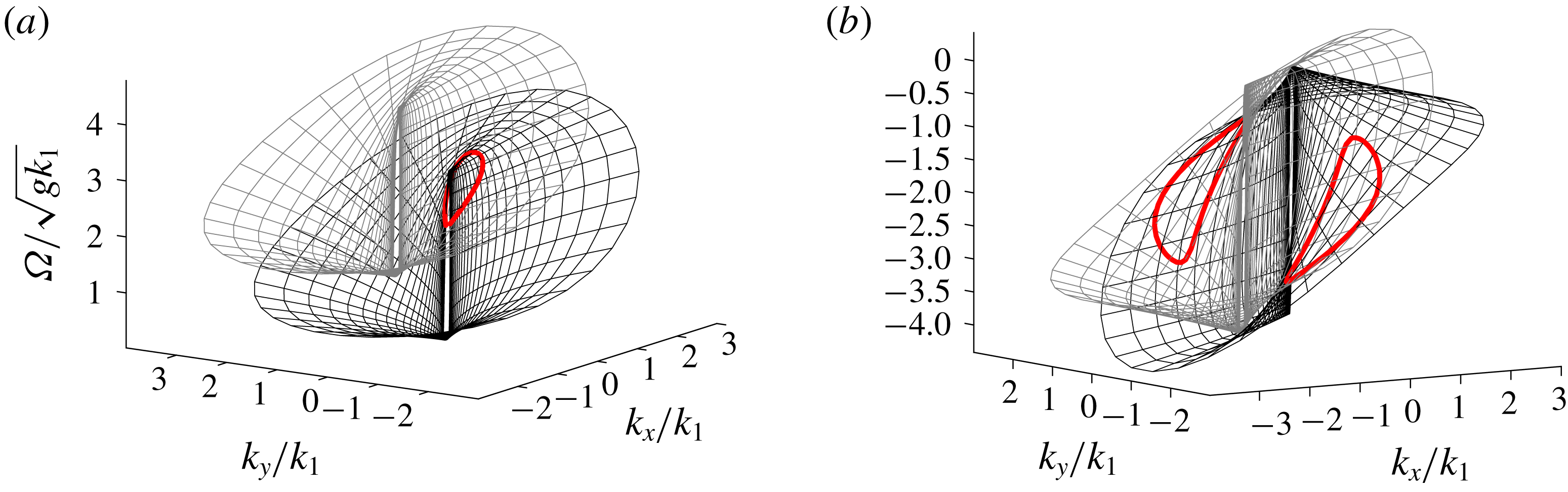
Gravity wave dispersion resonance is possible only at third order and above in irrotational flows (Phillips Reference Phillips1960; Kadomtsev & Karpman Reference Kadomtsev and Karpman1971), yet it is important to remember that dispersion resonance is possible at second order if the flow is three-dimensional and strongly sheared. Craik (Reference Craik1968) found such resonance to be remarkably powerful. To illustrate sheared triad resonance we visualise in figure 1
 $\unicode[STIX]{x1D6FA}$
-surfaces in
 $\boldsymbol{k}$
-space; surface intersection, and thus resonance, is possible if the shear-induced curve stretching disrupts the otherwise monotone curvature sufficiently. The shear strength (shear Froude number), the branch combination and the angle of the fixed wave vector
 $\boldsymbol{k}_{1}$
are the only parameters in these figures. A simple study of graph topography reveals that resonance for the weakest shear strength takes place as an interaction of two ‘plus’ or two ‘minus’ branches (figure 1
a), at
 $|S|=2\sqrt{gk_{1}}$
. This minimal shear triad is between two waves which are orthogonal to the shear and a third wave of large wavelength and high phase speed. (Note that such minima are sensitive to the scaling; Craik (Reference Craik1968), studying a special case, finds a minimum to occur at an intermediate angle as he scales with
 $\sqrt{gk_{1x}}$
as opposed to
 $\sqrt{gk_{1}}$
.) Opposing branch resonance (figure 1
b) first occurs at
 $|S|\approx 3.47\sqrt{gk_{1}}$
and involves a triad where
 $\boldsymbol{k}_{1}$
is near an angle
 $\unicode[STIX]{x03C0}/6$
to the current. Resonance at
 $\boldsymbol{k}_{1}$
-angels lower than this appears with only slight increased shear strength; figure 1(b) shows a case of slightly stronger shear with
 $\boldsymbol{k}_{1}$
parallel to the shear current.
Two dispersion relation curve branches in
 $\boldsymbol{k}$
-space are shown in each image, the origin of one surface shifted to a point
 $\boldsymbol{k}_{1}$
atop the other. The shifted surface thus shows
 $\unicode[STIX]{x1D714}=\unicode[STIX]{x1D6FA}_{\pm }\left(\boldsymbol{k}_{1}\right)\,+\unicode[STIX]{x1D6FA}_{+}\left(\boldsymbol{k}\right)\,$
for
 $\boldsymbol{k}_{1}$
fixed. Triad resonance occurs if, for any angle of
 $\boldsymbol{k}_{1}$
, there exists an intersection cut between the two surfaces; along such a cut
 $\boldsymbol{k}_{3}$
there exists pairs
 $\boldsymbol{k}_{1},\boldsymbol{k}_{2}$
satisfying
 $\unicode[STIX]{x1D6FA}_{\pm }\left(\boldsymbol{k}_{3}\right)\,=\unicode[STIX]{x1D6FA}_{\pm }\left(\boldsymbol{k}_{1}\right)\,+\unicode[STIX]{x1D6FA}_{+}\left(\boldsymbol{k}_{2}\right)\,$
. (a)
 $++$
branch combination,
 $S=-3.0\sqrt{gk_{1}}$
, angle
 $\boldsymbol{k}_{1}$
:
 $\unicode[STIX]{x03C0}/2$
. (b)
 $-+$
branch combination,
 $S=-3.75\sqrt{gk_{1}}$
, angle
 $\boldsymbol{k}_{1}$
:
 $\unicode[STIX]{x03C0}$
.

4.2 Advective resonance
A different type of resonance is possible from within the flow field. Where the dispersion resonance originates from a wave–wave interaction at the surface, advective resonance comes about when energy is transferred to the wave field from the background shear current
 $U(z)$
. It occurs where the phase velocity of a wave matches the shear advection velocity in the
 $x$
-direction. This mode of resonance is seen repeatedly in the velocity field expressions, e.g. (4.7), in the form of factors such as (4.2) resulting in terms diverging linearly with time. It is further auspicious to distinguish between two types of advective resonant behaviour. One appears in the form of critical layers at all depths
 $z=\unicode[STIX]{x1D709}_{i}$
where
 $\unicode[STIX]{x1D714}_{i}=k_{i,x}Sz$
. Vertical velocities remain continuous across the critical layers (due to the
 $\sinh$
in (4.7)), although the vertical velocity pertaining to the dispersive wave seen alone has a kink (discontinuous
 $z$
-derivative) here. The advective wave serves to cancel this kink initially so that the net vertical velocity is smooth across the critical layer but evolves into a kink as
 $t\rightarrow \infty$
. Horizontal velocities, presented in appendix A, will grow like
 $\boldsymbol{u}_{h}\sim t\,\text{e}^{-\text{i}\unicode[STIX]{x1D714}t}$
in a diverging manner near the critical layer and evolve towards a discontinuous singularity as
 $t\rightarrow \infty$
. The number of critical layers increases with the solution order. Just above or below a critical layer the flow remains periodic and bounded.
Another type of advective resonance occurs when
 $k_{x}$
and
 $\unicode[STIX]{x1D714}$
each tends to zero independently. The resonance
 $\bar{\unicode[STIX]{x1D714}}\rightarrow 0$
then occurs globally. This type of resonance has been famously proposed to act as a key mechanism for the phenomenon of Langmuir circulation, in turn, a vital mechanism for boundary layer mixing and the location and structure of the thermocline in oceans and lakes (Leibovich Reference Leibovich1983; Craik Reference Craik1986). We will return to this phenomenon later in § 6.1. In the confines of the initial value problem there is, for moderate times, no ambiguity near a global advective resonance – in fact, this was the main motivation for demanding irrotational initial condition. There is therefore no need for excluding the parts of the interaction spectrum where
 $k_{x}=k_{1x}+k_{2x}$
is small, as done by Zakharov & Shrira (Reference Zakharov and Shrira1990).
Note that all the terms associated with nonlinear advective resonance contain the factor
 $(\boldsymbol{k}_{1}\times \boldsymbol{k}_{2})_{z}$
, and so are artefacts of oblique wave interactions. The same is true for the appearance of all exponential integrals.
Our scope is restricted to currents of linear depth dependence, hence we have excluded the possibility of a final type of resonance, which is due to the curvature of
 $U(z)$
(Drazin & Reid Reference Drazin and Reid2004). Such resonances are possible in free surface flows even when there are no inflection points. One may refer to Shrira (Reference Shrira1993) who derived a perturbation series solution for linearised wave fields atop arbitrary, weak shear currents to any prescribed accuracy. Instabilities related to critical layers are found. Drivas & Wunsch (Reference Drivas and Wunsch2016) provide, with their study of a bilinear shear current of finite penetration depth, a related example of three-dimensional triad instability which is related to the current profile ‘kink’. Carpenter et al. (Reference Carpenter, Tedford, Heifetz and Lawrence2011) provide a review for two-dimensional homogeneous and density stratified shear flows.
5 Fluid particle trajectories
As is well known, the second-order Stokes expansion of a steady periodic wave creates a net mass transport in the direction of propagation, referred to as Stokes drift. From a Lagrangian perspective, the trajectories of individual fluid particles are not closed but is slightly shifted for each cycle. Naturally a similar phenomenon will be present in the presence of a transient wave such as may be created by an initial disturbance.
Surprisingly to us, the literature on fluid particle trajectories and Stokes drift in the presence of a uniform shear current has been found to be scarce; Kishida & Sobey (Reference Kishida and Sobey1988) provide expressions for monochromatic two-dimensional flow, but we are not aware of any literature for monochromatic waves propagating at oblique angles with a sheared current, nor of any reliable expressions for particle trajectories in sheared flow. The following theory has therefore been kept rather general, allowing for both monochromatic waves and discrete and continuous wave spectra.
We define a fluid particle trajectory
 $\hat{\boldsymbol{x}}_{p}\left(t\right)\,=(\hat{x}_{p}\left(t\right)\,,{\hat{y}}_{p}\left(t\right)\,,\hat{z}_{p}\left(t\right)\,)$
as the parametric position of an imaginary particle whose velocity always coincides with the velocity field at the immediate trajectory position. Precisely,
 $$\begin{eqnarray}{\displaystyle \frac{\text{d}\hat{\boldsymbol{x}}_{p}}{\text{d}t}}=\hat{\boldsymbol{u}}\left(\hat{\boldsymbol{x}}_{p}\left(t\right)\,,t\right)\,\!,\end{eqnarray}$$
where the initial particle position is close to a point
 $\boldsymbol{x}_{0}=(x_{0},y_{0},z_{0})$
at
 $t=0$
. Assume that
 $\boldsymbol{x}_{p}$
revolves around an orbit centre point
 $\hat{\boldsymbol{x}}_{s}$
which slides in the horizontal plane with a constant velocity
 $\hat{\unicode[STIX]{x1D74A}}_{s}$
. Taylor expanding
 $\hat{\boldsymbol{u}}$
about
 $\hat{\boldsymbol{x}}_{s}$
generates, in index notation,
 $$\begin{eqnarray}\hat{u} _{i}\left(\hat{\boldsymbol{x}}_{p}\left(t\right)\,,t\right)\,\approx (\hat{u} _{i})_{s}+(\hat{\boldsymbol{x}}_{p}-\hat{\boldsymbol{x}}_{s})(\hat{\unicode[STIX]{x1D735}}\hat{u} _{i})_{s}^{\text{T}}+{\textstyle \frac{1}{2}}(\hat{\boldsymbol{x}}_{p}-\hat{\boldsymbol{x}}_{s})(\hat{\unicode[STIX]{x1D735}}\hat{\unicode[STIX]{x1D735}}\hat{u} _{i})_{s}(\hat{\boldsymbol{x}}_{p}-\hat{\boldsymbol{x}}_{s})^{\text{T}}+\cdots \,,\end{eqnarray}$$
where
 $s$
-suffixes indicate evaluation at
 $\boldsymbol{x}=\hat{\boldsymbol{x}}_{s}$
. Inserting (5.2) into (5.1) makes
 $\hat{\boldsymbol{x}}_{p}$
a Stokes series expansion with increasing number of nested convolutions in the form of (3.2). We use the sliding orbit
 $\hat{\boldsymbol{x}}_{s}$
to remove linear time dependencies in
 $\hat{\boldsymbol{x}}_{p}$
(from current advection and Stokes drift) from the right-hand side of (5.2), denying
 $\hat{\boldsymbol{x}}_{p}$
higher polynomials in time in the subsequent orders. Consequently, also
 $\hat{\boldsymbol{x}}_{s}$
takes the form of a Stokes expansion. The procedure is analogous to the well-known frequency perturbation of the Poincaré–Lindstedt method. At zeroth order, equation (5.2) then yields
 $$\begin{eqnarray}\boldsymbol{x}_{p}^{(0)}\left(t\right)\,=\boldsymbol{x}_{s}^{(0)}\left(t\right)\,=\boldsymbol{x}_{0}+Sz_{0}\boldsymbol{e}_{x}t,\end{eqnarray}$$
as expected.
Evaluation of the perturbation velocity field along the sliding orbit
 $\hat{\boldsymbol{x}}_{s}$
is equivalent to a Galilean transformation and generates a Doppler shift
 $$\begin{eqnarray}\hat{\boldsymbol{u}}\left(\hat{\boldsymbol{x}}_{s}\left(t\right)\,,t\right)\,=\hat{\boldsymbol{u}}_{s}\left(t\right)\,\rightarrow \boldsymbol{u}_{s}\left(t\right)\,=\boldsymbol{u}\left(t\right)\,\text{e}^{\text{i}\boldsymbol{k}\boldsymbol{\cdot }\hat{\unicode[STIX]{x1D74A}}_{s}t}\end{eqnarray}$$
in Fourier space.
 $\boldsymbol{x}_{0}$
is here the independent variable of the corresponding inverse Fourier transform. A cascade of ordinary differential equations,
 $$\begin{eqnarray}\displaystyle & & \displaystyle {\displaystyle \frac{\text{d}x_{\text{p},i}}{\text{d}t}}-Sz_{p}\unicode[STIX]{x1D6FF}_{i,1}=u_{\text{s},i}\nonumber\\ \displaystyle & & \displaystyle \qquad +\,\left[\text{i}\unicode[STIX]{x1D714}_{s}x_{\text{p},i}+(\boldsymbol{x}_{p}-\boldsymbol{x}_{s})(\unicode[STIX]{x1D735}u_{\text{s},i})^{\text{T}}+{\textstyle \frac{1}{2}}(\boldsymbol{x}_{p}-\boldsymbol{x}_{s})(\unicode[STIX]{x1D735}\unicode[STIX]{x1D735}u_{\text{s},i})(\boldsymbol{x}_{p}-\boldsymbol{x}_{s})^{\text{T}}+\right]\!,\end{eqnarray}$$
results for the subsequent orders. (Only interaction terms of the appropriate combined order enter among the inhomogeneous interaction terms in the square brackets on the right-hand side.) The first bracket term, where
 $$\begin{eqnarray}\unicode[STIX]{x1D714}_{s}=\unicode[STIX]{x1D714}-\boldsymbol{k}\boldsymbol{\cdot }\hat{\unicode[STIX]{x1D74A}}_{s},\end{eqnarray}$$
originates from incorporating the Stokes drift into particle orbit position and becomes active at third order.
Non-zero contributions to the sliding orbit velocity
 $\unicode[STIX]{x1D74A}_{s}$
are found at even orders where the time dependency in self-interacting waves cancel. Physically, this signifies the phenomenon of Stokes drift. Such contributions appear as finite terms when working with monochromatic waves or discrete wave spectra. In a continuous wave spectrum
 $\hat{\unicode[STIX]{x1D74A}}_{s}\rightarrow 0$
at all non-zero orders. Instead, Stokes drift then manifests as poles whose limits generate linear time dependency in the manner of (4.2).
To first order, equation (5.5) yields
 $$\begin{eqnarray}\boldsymbol{x}_{p}^{(1)}={\displaystyle \frac{\text{i}}{\unicode[STIX]{x1D714}_{s}^{(0)}}}\left(\boldsymbol{u}_{s}^{(1)}+{\displaystyle \frac{\text{i}}{\unicode[STIX]{x1D714}_{s}^{(0)}}}Sw_{s}^{(1)}\boldsymbol{e}_{x}\right),\end{eqnarray}$$
with
 $\unicode[STIX]{x1D714}_{s}^{(0)}=\unicode[STIX]{x1D714}-k_{x}Sz_{0}$
. Summation over the two frequency branches of the first-order wave field is implied;
 $\boldsymbol{x}_{p}^{(1)}$
contains only terms which are periodic in time and so
 $\unicode[STIX]{x1D74A}_{s}^{(1)}=\mathbf{0}$
.
A simple study of (5.7) reveals that the second term serves to make the first-order trajectories elliptical as a result of the linearly differing current advection above and below the orbit centre. We remark that this simple mechanism is not present in the solution presented by Hsu (Reference Hsu2013). Likewise, Stokes drift does not appear to be present in Umeyama, Shintani & Watanabe (Reference Umeyama, Shintani and Watanabe2011). We further note that our particle trajectory approximation contains critical layers, even in the two-dimensional (2-D) case where the velocity field itself is overall smooth. This is because particle oscillation ceases if the advection causes the wave crest to remain stationary relative to the particle orbit. Elliptical shear stretching thus increases near critical layers and our trajectory approximation ceases to be valid if the trajectory orbit and the critical layer are too close.
The spectral expressions for the second-order trajectory are similar to (5.7) in appearance but decidedly bulkier, and we do not quote them explicitly. Instead, because they seem absent in the present literature, we quote to second order our result for velocity field and fluid particle position in a monochromatic wave propagating at an oblique angle to a current of uniform vorticity at finite depth. This has been calculated with the above procedure for validation purposes. Introducing dimensionless parameters
 $$\begin{eqnarray}\unicode[STIX]{x1D716}=\unicode[STIX]{x1D702}k;\quad \tilde{\boldsymbol{k}}={\displaystyle \frac{\boldsymbol{k}}{k}};\quad \tilde{S}=\unicode[STIX]{x1D6FD}{\displaystyle \frac{k_{x}}{k}}{\displaystyle \frac{S}{\bar{\unicode[STIX]{x1D714}}}};\quad \tilde{S}_{0}=\unicode[STIX]{x1D6FD}_{0}{\displaystyle \frac{k_{x}}{k}}{\displaystyle \frac{S}{\unicode[STIX]{x1D714}_{s}^{(0)}}};\quad \tilde{A}={\displaystyle \frac{k^{2}A}{\unicode[STIX]{x1D714}_{s}^{(0)}}}\end{eqnarray}$$
and the orthogonal wave vector
 $\boldsymbol{k}_{\bot }=(-k_{y},k_{x})^{\text{T}}$
, the velocity field of a monochromatic wave with wave vector
 $\boldsymbol{k}$
and frequency
 $\unicode[STIX]{x1D714}$
reads
 $$\begin{eqnarray}\displaystyle & & \displaystyle \hat{\boldsymbol{u}}_{h}=Sz\boldsymbol{e}_{x}+{\displaystyle \frac{\unicode[STIX]{x1D716}A^{(1)}}{\sqrt{1-\unicode[STIX]{x1D6FD}^{2}}}}\left(\tilde{\boldsymbol{k}}+\tilde{\boldsymbol{k}}_{\bot }{\displaystyle \frac{k_{y}}{k_{x}}}\tilde{S}\right)\cos (\boldsymbol{r}\boldsymbol{\cdot }\boldsymbol{k}-\unicode[STIX]{x1D714}t)\nonumber\\ \displaystyle & & \displaystyle \quad +\,{\displaystyle \frac{\unicode[STIX]{x1D716}^{2}}{1-\unicode[STIX]{x1D6FD}^{2}}}\left\{A^{(2)}\left[\tilde{\boldsymbol{k}}(1+\unicode[STIX]{x1D6FD}^{2})+\tilde{\boldsymbol{k}}_{\bot }{\displaystyle \frac{k_{y}}{k_{x}}}\tilde{S}\right]-{\displaystyle \frac{\tilde{\boldsymbol{k}}_{\bot }}{4}}{\displaystyle \frac{k}{\bar{\unicode[STIX]{x1D714}}}}\left(A^{(1)}\right)^{2}{\displaystyle \frac{k_{y}}{k_{x}}}\tilde{S}^{2}\right\}\cos 2(\boldsymbol{k}\boldsymbol{\cdot }\boldsymbol{r}-\unicode[STIX]{x1D714}t)\qquad \quad\end{eqnarray}$$
 $$\begin{eqnarray}\displaystyle & & \displaystyle {\hat{w}}=\unicode[STIX]{x1D716}A^{(1)}{\displaystyle \frac{\unicode[STIX]{x1D6FD}}{\sqrt{1-\unicode[STIX]{x1D6FD}^{2}}}}\sin (\boldsymbol{k}\boldsymbol{\cdot }\boldsymbol{r}-\unicode[STIX]{x1D714}t)+\unicode[STIX]{x1D716}^{2}A^{(2)}{\displaystyle \frac{2\unicode[STIX]{x1D6FD}}{1-\unicode[STIX]{x1D6FD}^{2}}}\sin 2(\boldsymbol{k}\boldsymbol{\cdot }\boldsymbol{r}-\unicode[STIX]{x1D714}t)\end{eqnarray}$$
 $$\begin{eqnarray}A^{(1)}={\displaystyle \frac{\unicode[STIX]{x1D714}}{k}}{\displaystyle \frac{\sqrt{1-\unicode[STIX]{x1D6FD}^{2}}}{\unicode[STIX]{x1D6FD}}}\bigg|_{z=0},\quad A^{(2)}={\displaystyle \frac{\unicode[STIX]{x1D714}}{k}}{\displaystyle \frac{1-\unicode[STIX]{x1D6FD}^{2}}{4\unicode[STIX]{x1D6FD}^{4}}}\left[3\left(1-\unicode[STIX]{x1D6FD}^{2}+\tilde{S}\right)+\tilde{S}^{2}\right]\bigg|_{z=0},\end{eqnarray}$$
which agrees with the field quoted by Hsu et al. (Reference Hsu, Francius, Montalvo and Kharif2016) in two dimensions. This generates the fluid particle trajectories
 $$\begin{eqnarray}\displaystyle \hat{\boldsymbol{r}}_{p} & = & \displaystyle \boldsymbol{r}_{0}+Sz_{0}\boldsymbol{e}_{x}t-{\displaystyle \frac{\unicode[STIX]{x1D716}\tilde{A}^{(1)}}{k}}{\displaystyle \frac{\tilde{\boldsymbol{k}}}{\sqrt{1-\unicode[STIX]{x1D6FD}_{0}^{2}}}}(1+\tilde{S}_{0})\sin (\boldsymbol{k}\boldsymbol{\cdot }\boldsymbol{r}_{0}-\unicode[STIX]{x1D714}_{s}t)\nonumber\\ \displaystyle & & \displaystyle -\,{\displaystyle \frac{\unicode[STIX]{x1D716}^{2}}{2k}}{\displaystyle \frac{\tilde{\boldsymbol{k}}}{1-\unicode[STIX]{x1D6FD}_{0}^{2}}}\left[\tilde{A}^{(2)}(1+\unicode[STIX]{x1D6FD}_{0}^{2}+\tilde{S}_{0})-{\displaystyle \frac{1}{2}}(\tilde{A}^{(1)})^{2}\left(1-\unicode[STIX]{x1D6FD}_{0}^{2}+\tilde{S}_{0}+{\displaystyle \frac{{\tilde{S}_{0}}^{2}}{2}}\right)\!\right]\!\sin 2(\boldsymbol{k}\boldsymbol{\cdot }\boldsymbol{r}_{0}-\unicode[STIX]{x1D714}_{s}t)\nonumber\\ \displaystyle & & \displaystyle +\,{\displaystyle \frac{\unicode[STIX]{x1D716}^{2}}{2k}}{\displaystyle \frac{1}{1-\unicode[STIX]{x1D6FD}_{0}^{2}}}(\tilde{A}^{(1)})^{2}\left[\tilde{\boldsymbol{k}}(1+\unicode[STIX]{x1D6FD}_{0}^{2}+\tilde{S}_{0})+2\tilde{\boldsymbol{k}}_{\bot }{\displaystyle \frac{k_{y}}{k_{x}}}\tilde{S}_{0}(1+\tilde{S}_{0})\right]\unicode[STIX]{x1D714}_{s}^{(0)}t\end{eqnarray}$$
 $$\begin{eqnarray}\displaystyle \hat{z}_{p} & = & \displaystyle z_{0}+{\displaystyle \frac{\unicode[STIX]{x1D716}\tilde{A}^{(1)}}{k}}{\displaystyle \frac{\unicode[STIX]{x1D6FD}_{0}}{\sqrt{1-\unicode[STIX]{x1D6FD}_{0}^{2}}}}\cos (\boldsymbol{k}\boldsymbol{\cdot }\boldsymbol{r}_{0}-\unicode[STIX]{x1D714}_{s}t)\nonumber\\ \displaystyle & & \displaystyle +\,{\displaystyle \frac{\unicode[STIX]{x1D716}^{2}}{k}}{\displaystyle \frac{1}{1-\unicode[STIX]{x1D6FD}_{0}^{2}}}\left[\tilde{A}^{(2)}-{\displaystyle \frac{1}{4}}(\tilde{A}^{(1)})^{2}\tilde{S}_{0}\right]\cos 2(\boldsymbol{k}\boldsymbol{\cdot }\boldsymbol{r}_{0}-\unicode[STIX]{x1D714}_{s}t)\end{eqnarray}$$
 $\unicode[STIX]{x1D6FD}=\tanh k(z+d)$
and
 $\unicode[STIX]{x1D6FD}_{0}=\tanh k(z_{0}+d)$
are the bathymetry parameters for a depth
 $d$
; at infinite depth we first insert (5.10) and then take the limit
 $\unicode[STIX]{x1D6FD},\unicode[STIX]{x1D6FD}_{0}\rightarrow 1$
, noting that
 $(1-\unicode[STIX]{x1D6FD}^{2}|_{z=0})/(1-\unicode[STIX]{x1D6FD}_{0}^{2})\rightarrow \exp 2kz_{0}$
. The last expression in (5.11a
) adheres to the Stokes drift and is non-periodic. Following the described procedure we put
 $\boldsymbol{x}_{s}^{(2)}$
equal to this expression when proceeding to third order, removing the quadratic time dependency otherwise appearing there. Again, our Stokes drift expression contains several shear-dependent terms not reported in Hsu (Reference Hsu2013). It has been verified numerically that the code used to compute the results of § 6.2 reproduces the above result at infinite depth when perturbing the bound frequency with an imaginary component
 $\text{i}\unicode[STIX]{x1D700}$
in the manner
 $$\begin{eqnarray}\hat{\boldsymbol{r}}_{p}^{(2)}\sim \lim _{\unicode[STIX]{x1D700}\rightarrow 0^{+}}\left({\displaystyle \frac{\text{e}^{-\text{i}(\unicode[STIX]{x1D714}_{s}-\text{i}\unicode[STIX]{x1D700})t}}{\unicode[STIX]{x1D714}_{s}-\text{i}\unicode[STIX]{x1D700}}}+{\displaystyle \frac{\text{i}\unicode[STIX]{x1D700}}{(\unicode[STIX]{x1D714}_{s}-\text{i}\unicode[STIX]{x1D700})^{2}}}\right)\xrightarrow[{}]{\unicode[STIX]{x1D714}_{s}=0}\lim _{\unicode[STIX]{x1D700}\rightarrow 0^{+}}{\displaystyle \frac{\text{e}^{-\unicode[STIX]{x1D700}t}-1}{\text{i}\unicode[STIX]{x1D700}}}=-\text{i}t.\end{eqnarray}$$
The term which is time independent is a sagaciously chosen integration constant which appears when evaluating (5.5); it appropriately balances the singularity while vanishing from
 $\unicode[STIX]{x1D714}_{s}=0$
.
Finally, we remark that a uniform current can easily be incorporated into these results by linearly shifting the frame of reference in the manner
 $$\begin{eqnarray}\displaystyle \hat{\boldsymbol{U}}\left(\boldsymbol{x},t\right)\, & = & \displaystyle \hat{\boldsymbol{u}}\left(\boldsymbol{x}-\boldsymbol{U}_{0}t,t\right)\,+\boldsymbol{U}_{0},\end{eqnarray}$$
 $$\begin{eqnarray}\displaystyle \hat{\boldsymbol{X}}_{p}\left(t\right)\, & = & \displaystyle \hat{\boldsymbol{x}}_{p}\left(t\right)\,+\boldsymbol{U}_{0}t,\end{eqnarray}$$
 $\hat{\boldsymbol{U}}$
and
 $\hat{\boldsymbol{X}}_{p}$
are now the velocity field and fluid particle trajectory in the presence of a uniform current with velocity
 $\boldsymbol{U}_{0}$
, respectively; choosing
 $\boldsymbol{U}_{0}=Sd$
in (5.9b
)–(5.11b
) implies zero current velocity at the bottom surface. The effect of uniform currents on the particle trajectory was investigated by Constantin & Strauss (Reference Constantin and Strauss2010).
6 Numerical examples
6.1 Generalised Langmuir vortices from obliquely incident wave trains
The resonance of (4.7) as
 $\unicode[STIX]{x1D714}=0$
and
 $k_{x}=0$
was first proposed as a mechanism for Langmuir-type vortices in a model by Benney & Lin (Reference Benney and Lin1960), later investigated numerically by Antar & Collins (Reference Antar and Collins1975). The presence of these large rollers can sometimes be observed in the form of parallel ‘windrows’ forming in the wind direction on oceans and lakes due to the gathering of seaweed and flotsam in the downwelling regions they create.
Presently we consider an inviscid model proposed by Craik (Reference Craik1970) in which we consider a pair of plane waves whose wave vectors are oblique to, and symmetrical about, the
 $x$
-axis; a train moving in the direction
 $\boldsymbol{k}_{\text{L}+}=(k_{\text{L}x},k_{\text{L}y})^{\text{T}}$
and another in the direction
 $\boldsymbol{k}_{\text{L}-}=(k_{\text{L}x},-k_{\text{L}y})^{\text{T}}$
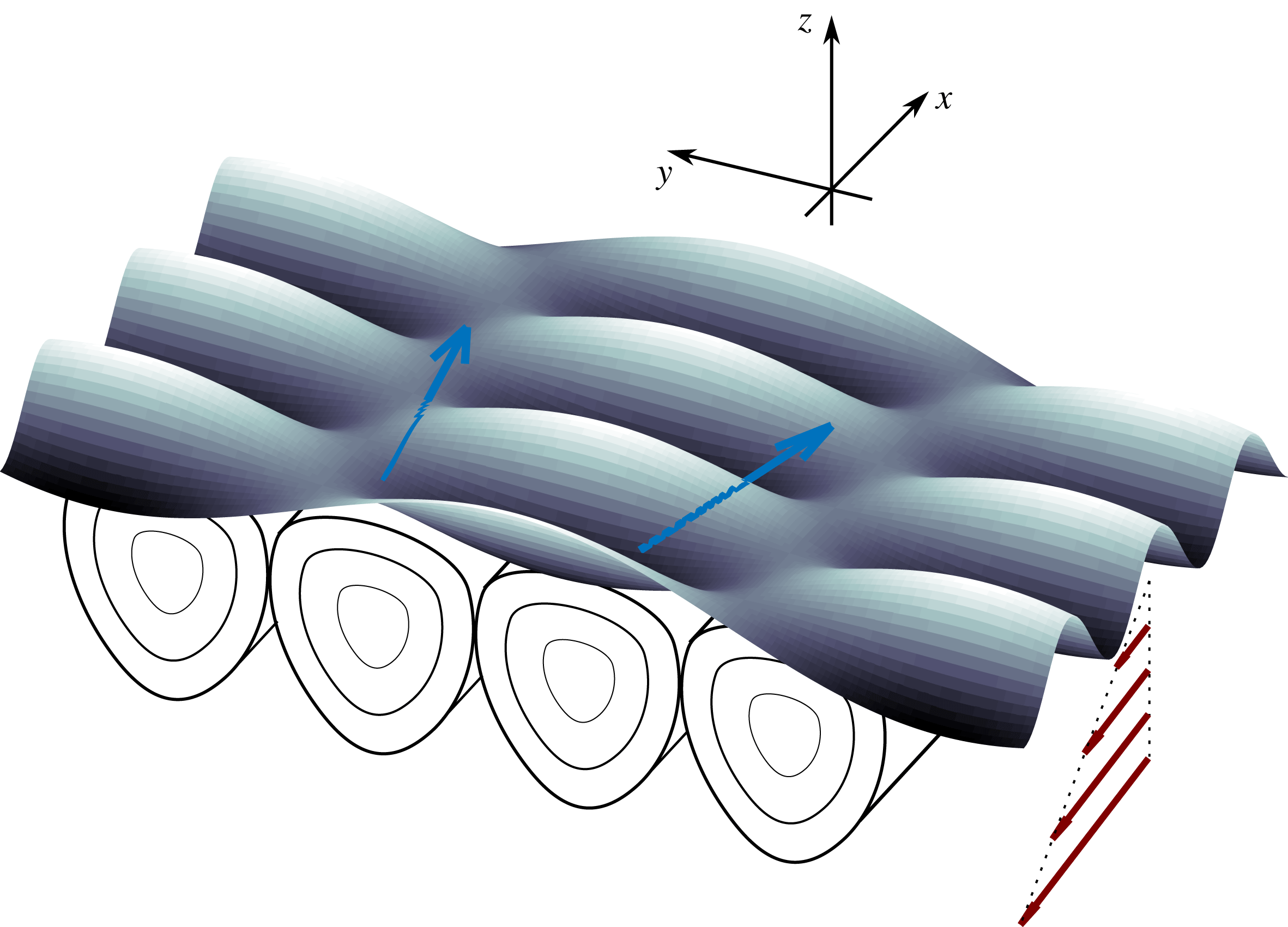
. The set-up is sketched in figure 2. Remember that we work in a frame of reference moving with the water surface. In the laboratory frame this would most likely represent waves propagating along with the surface flow, e.g. if the model should mimic a surface current created by the wind.
Such a case is represented with the first-order spectrum
 $$\begin{eqnarray}\unicode[STIX]{x1D701}_{\pm }^{(1)}(\boldsymbol{k})=2\unicode[STIX]{x1D702}\unicode[STIX]{x03C0}^{2}\mathop{\sum }_{\unicode[STIX]{x1D70E}=\pm }\unicode[STIX]{x1D6FF}\left(\boldsymbol{k}\mp \boldsymbol{k}_{L\unicode[STIX]{x1D70E}}\right)\,\!,\end{eqnarray}$$
 $\unicode[STIX]{x1D6FF}$
being the Dirac delta function and
 $\unicode[STIX]{x1D702}$
the wave amplitude. The second-order (bound) waves are then of the form
 $$\begin{eqnarray}\displaystyle \hat{\unicode[STIX]{x1D701}}^{(2)} & = & \displaystyle \mathop{\sum }_{\unicode[STIX]{x1D70E}_{1},\unicode[STIX]{x1D70E}_{2}=\pm }\int {\displaystyle \frac{\text{d}\boldsymbol{k}_{1}\text{d}\boldsymbol{k}_{2}}{(2\unicode[STIX]{x03C0})^{4}}}\unicode[STIX]{x1D701}_{\unicode[STIX]{x1D70E}_{1}}^{(1)}\left(\boldsymbol{k}_{1}\right)\,\unicode[STIX]{x1D701}_{\unicode[STIX]{x1D70E}_{2}}^{(1)}\left(\boldsymbol{k}_{2}\right)\,[\cdots \!\,]\text{e}^{\text{i}(\boldsymbol{k}\boldsymbol{\cdot }\boldsymbol{r}-\unicode[STIX]{x1D714}t)}\nonumber\\ \displaystyle & = & \displaystyle {\displaystyle \frac{\unicode[STIX]{x1D702}^{2}}{4}}\!\!\mathop{\sum }_{\unicode[STIX]{x1D70E}_{1},\unicode[STIX]{x1D70E}_{2},\unicode[STIX]{x1D70E}_{1}^{\prime },\unicode[STIX]{x1D70E}_{2}^{\prime }=\pm }\!\![\cdots \,]\,\text{e}^{\text{i}(\boldsymbol{k}\boldsymbol{\cdot }\boldsymbol{r}-\unicode[STIX]{x1D714}t)}\bigg|_{\substack{ \boldsymbol{k}_{1}=\unicode[STIX]{x1D70E}_{1}\boldsymbol{k}_{\text{L}\unicode[STIX]{x1D70E}_{1}^{\prime }} \\ \boldsymbol{k}_{2}=\unicode[STIX]{x1D70E}_{2}\boldsymbol{k}_{\text{L}\unicode[STIX]{x1D70E}_{2}^{\prime }}}}.\end{eqnarray}$$
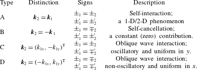
The sum runs over sixteen sign combinations. Half of these are duplicates where the wave indices are swapped, leaving eight distinct kernels. These in turn form pairs of complex conjugates, leaving four physically distinct types of two-wave interactions, as listed in table 1.
Geometry of the classic set-up originally considered by Craik (Reference Craik1970): two monochromatic waves (wave vectors illustrated with arrows) propagate symmetrically about the background shear flow. Langmuir vortices are created beneath the surface.

Four distinct types of interactions between two waves
 $\boldsymbol{k}_{1},\boldsymbol{k}_{2}$
of equal wavelength.

Types A and B do not entail any three-dimensional interaction and the oblique interaction term
 $w_{cross}$
, given in (4.11), disappears from (3.4) as
 $(\boldsymbol{k}_{1}\times \boldsymbol{k}_{2})_{z}\equiv 0$
in these cases. Type C is a wave interaction propagating in the
 $x$
-direction with frequency
 $2\unicode[STIX]{x1D714}_{+}\left(\boldsymbol{k}_{0}\right)\,$
. Our main interest lies in type D, whose particular interaction can set up vortical ‘roll’ structures parallel to the
 $x$
-axis, a candidate mechanism for Langmuir circulation. For type D,
 $\unicode[STIX]{x1D714}$
and
 $k_{x}$
are both zero, activating the resonance in (4.7) at all depths – the flow field solution component
 $w_{cross}$
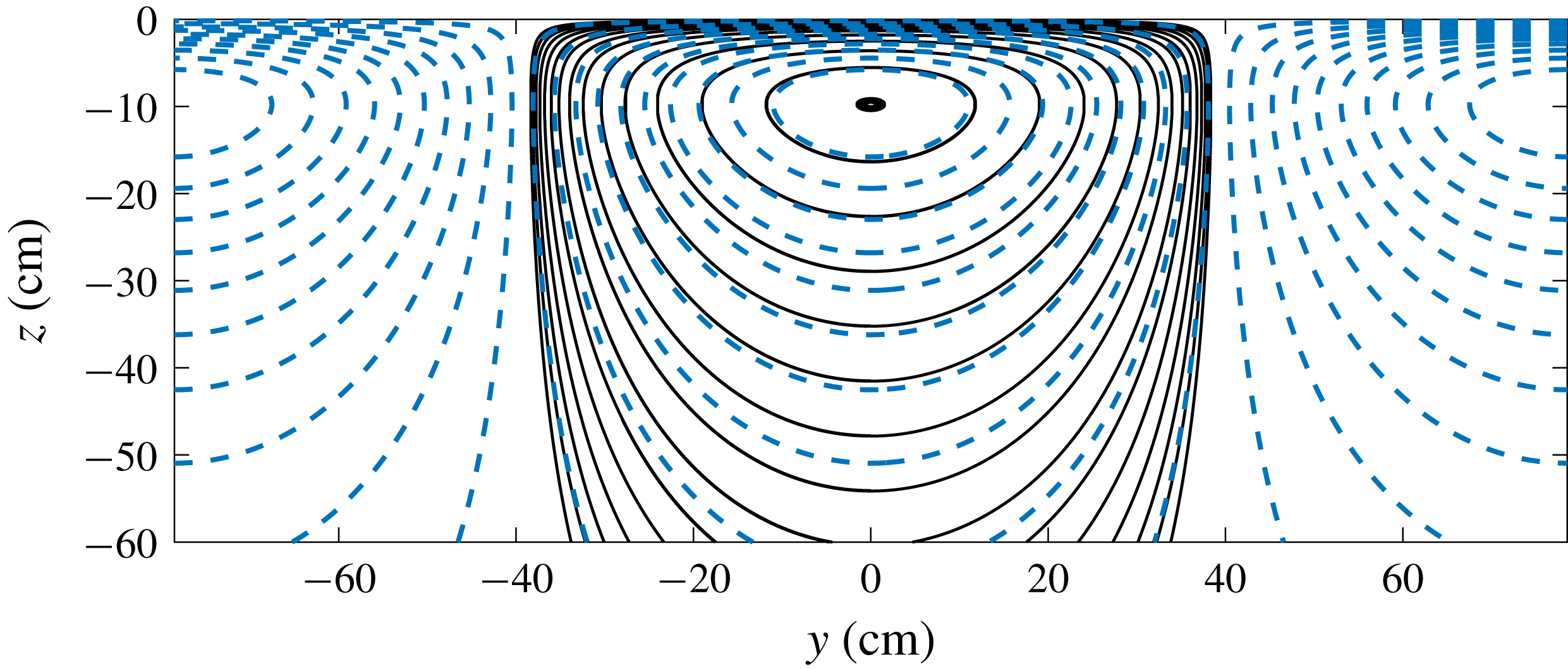
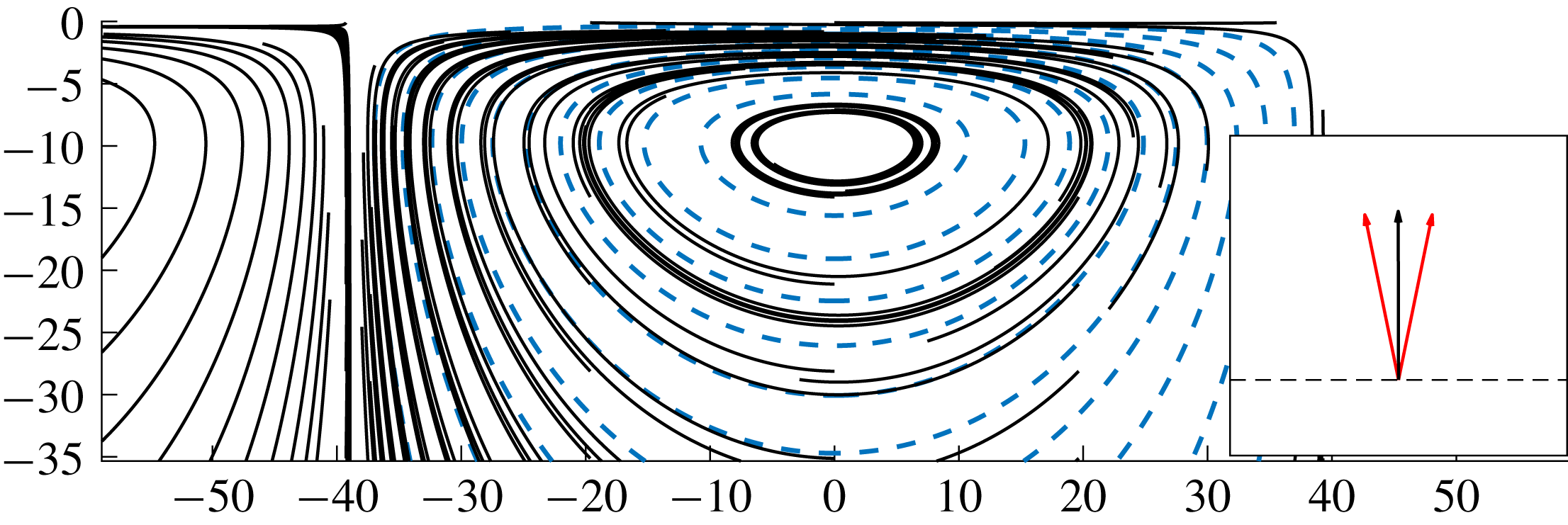
taking on a constant acceleration in inviscid theory. Figure 3 shows the flow field from interaction type D in the
 $yz$
-plane. Streamline plots of the velocity field for the special case presented in appendix B are here presented along with contours of the streamfunction solution (B 4b
) presented by Craik (Reference Craik1970). We mention here that the solution presented in said reference contains an error which is rectified in appendix B.
Langmuir vortex cells (wave interaction type D). Blue, stippled: streamlines from streamfunction (B 4b ) from Craik (Reference Craik1970). Black, solid: streamlines numerically computed from velocity field presented in appendix B. Flow state in given reference.

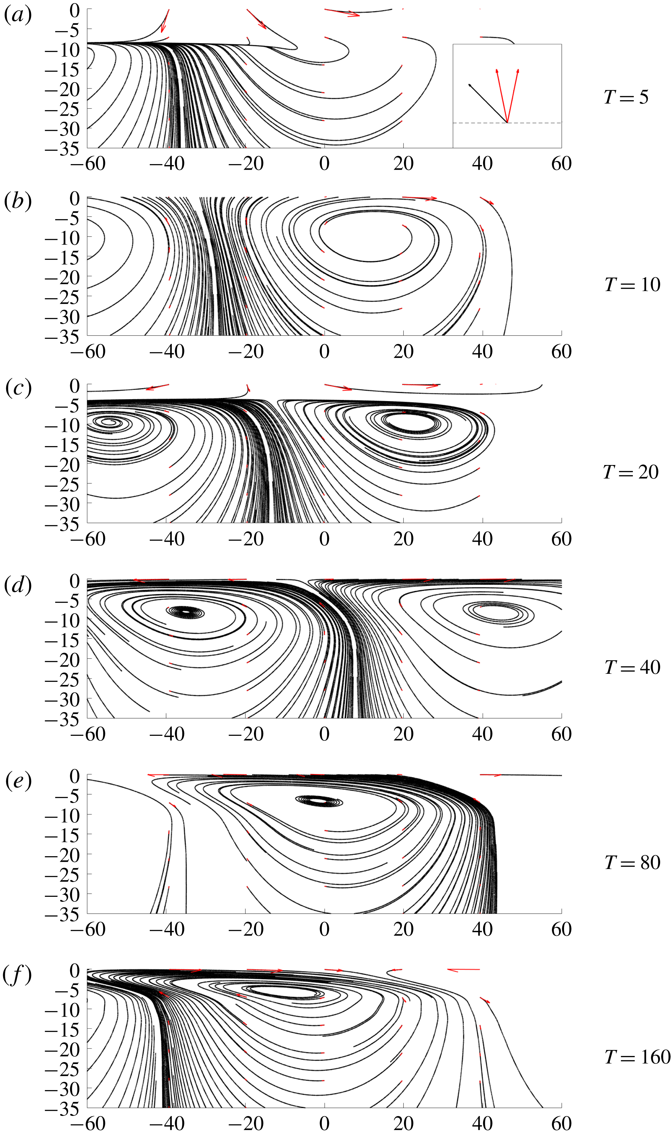
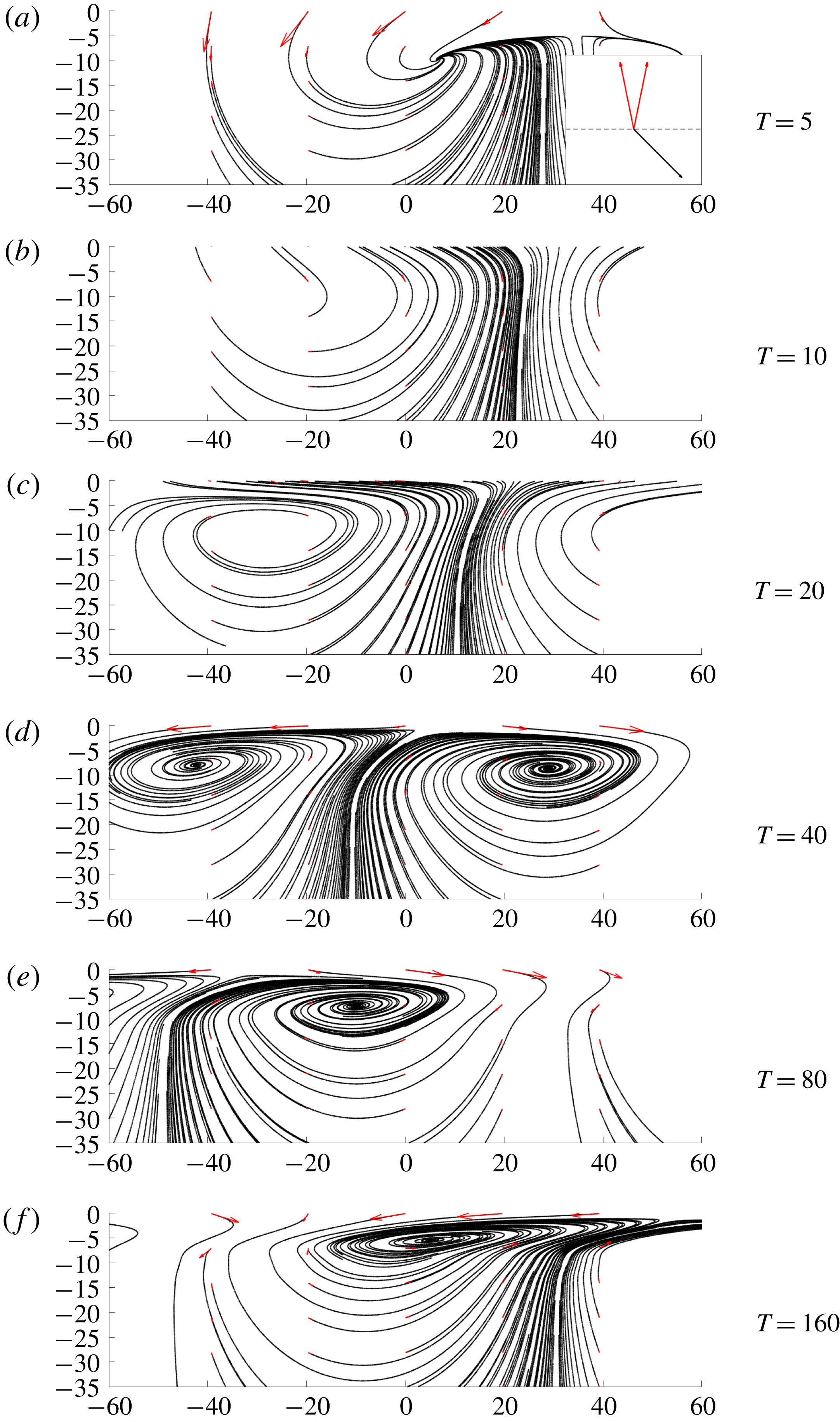
With the more general solution one can investigate this kind of set-up further. In figures 4–6 we rotate the direction of the shear current relative to the propagation direction of the wave pair. New dynamics is now observed. As time progresses the vortices evolve towards a similar profile as in the symmetric case but then slowly begin to skew in the direction of the shear flow until a steady vortex shape is reached. The rate of skewing of the vortex increases with the angle to the shear direction, but the evolution is insensitive to whether the
 $k$
-vectors point along or against the shear flow direction. This is shown in figures 4–5. Some periodic wave motion is initially prominent near the surface in these figures. At larger times this motion is hidden by the increasing vortex intensity. The dimensionless time is
 $T=t\sqrt{g/L}$
where
 $L=\unicode[STIX]{x03C0}/(2k_{\text{L}y})$
is the symmetric vortex width. Vortex structures are here aligned with
 $\boldsymbol{k}=\boldsymbol{k}_{1}+\boldsymbol{k}_{2}$
. (Interaction type D loses spatial dependence in
 $x$
in a coordinate system aligned with
 $\boldsymbol{k}$
.) All rolls will however uniformly drift sideways with time in the direction of the current.
Finally, figure 6, where the angle between
 $\boldsymbol{k}_{1}+\boldsymbol{k}_{2}$
and the
 $x$
-axis is
 $0.1^{\circ }$
and
 $T=100$
, demonstrates how the general solution converges towards Craik’s symmetric case solution.
The non-swirling interactions (types A–C) contribute with a limited periodic disturbance to the vortex motion, which initially dominates the second-order motion of figure 4–6 but is then overwhelmed by the vortex motion whose period is considerably longer. In the symmetric case (figure 3), this periodic motion is in time completely wiped out by the unbounded vortex motion. The driving force for the Langmuir circulation reduces as the angle between shear and mean wave direction approaches
 $90^{\circ }$
. At the same time the skewing mechanism intensifies. No Langmuir vortices are generated if the mean wave direction is perpendicular to the direction of the current. This is not dissimilar to the findings of Van Roekel et al. (Reference Van Roekel, Fox-Kemper, Sullivan, Hamlington and Haney2012) who performed large eddy simulations of the Craik–Leibovich equations with misaligned Stokes drift and wind forcing; their results show diminishing Langmuir turbulence as the angle between Stokes drift and Langmuir cell alignment is made to increase.
Slowly developing skewed Langmuir-like vortical structures due to a wave pair propagating, on average, at
 $45^{\circ }$
relative to the shear current. Streamlines are shown in the plane orthogonal to the vortex rolls illustrated with a dashed line in the inset in (a), where also the wave pair and current directions are indicated. (See movieFile1 and movieFile2 available at https://doi.org/10.1017/jfm.2018.960.)

Same as figure 4, but the angle between
 $\boldsymbol{k}$
and shear current is now
 $-135^{\circ }$
.

Angle
 $0.1^{\circ }$
between shear current and
 $\boldsymbol{k}$
,
 $T=100$
. Dashed lines: contours of the streamfunction (B 4b
) for angle
 $0^{\circ }$
from Craik (Reference Craik1970).

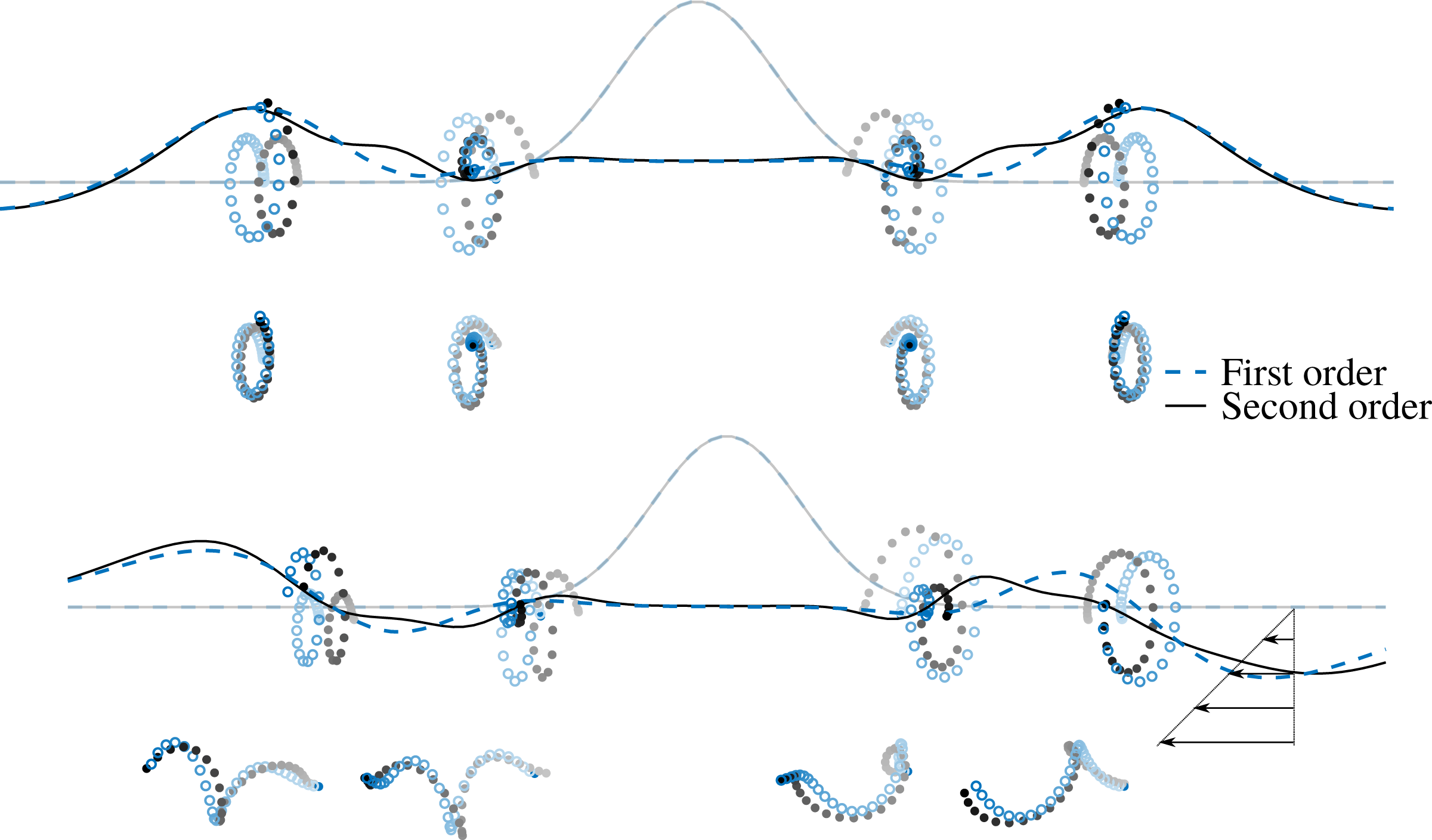
Two-dimensional Cauchy–Poisson problem – Gaussian initial elevation profile with ‘steepness’
 $H=0.2$
. Blue, dashed/open: first-order solution; black, solid/filled: second-order solution. (a)
 $\text{Fr}_{S}=0$
; (b)
 $\text{Fr}_{S}=0.5$
Surface elevation is plotted at
 $T=0$
and
 $T=6.0$
, together with particle positions within this time interval. Increasing opacity indicates the evolution in time. (See movieFile3 and movieFile4.)

6.2 Fluid particle trajectory beneath a localised disturbance in two dimensions
As we proceed towards spectral computations we start by considering a two-dimensional Cauchy problem. This is similar to the problem studied by Abou-Dina (Reference Abou-Dina2001) for cases of varying bathymetry. Two-dimensionality means that all wave vectors are parallel such that no oblique interaction between waves and shear can take place;
 $(\boldsymbol{k}_{1}\times \boldsymbol{k}_{2})_{z}\equiv 0$
. As a result, all the rotational cross-terms and advective terms disappear. We look at this problem including fluid particle trajectories.
Figure 7 shows the surface elevation and particle trajectories to second order. The initial surface elevation is here a Gaussian profile at rest,
 $$\begin{eqnarray}\hat{\unicode[STIX]{x1D701}}_{IC}=\unicode[STIX]{x1D702}\text{e}^{-\unicode[STIX]{x03C0}^{2}x^{2}/b^{2}}\quad \unicode[STIX]{x1D701}_{IC}=(\unicode[STIX]{x1D702}b/\sqrt{\unicode[STIX]{x03C0}})\text{e}^{-b^{2}k_{x}^{2}/(2\unicode[STIX]{x03C0})^{2}}\quad \dot{\hat{\unicode[STIX]{x1D701}}}_{IC}=\dot{\unicode[STIX]{x1D701}}_{IC}=0,\end{eqnarray}$$
and the surface pressure is uniform. Here
 $b$
is the Gaussian distribution width parameter. A respective dimensionless steepness, time and shear Froude number
 $$\begin{eqnarray}H=\unicode[STIX]{x1D702}/b,\quad T=t\sqrt{g/b},\quad \text{Fr}_{S}=S\sqrt{b/g},\end{eqnarray}$$
has here been introduced. Initial conditions have been chosen uniform in the
 $y$
-direction, although no significant complexity is added by letting the waves disperse at an angle to the shear current beyond the fact that also the vorticity field will be perturbed in this case (Ellingsen Reference Ellingsen2016). The procedure of perturbing the bound frequency, described in and around (5.12), is employed to avoid pole singularities appearing with self-interacting wave components at second order. As opposed to the linear solution, this shifts the second-order orbits of the particle trajectories as the main wave bulk flushes past. This is the transient manifestation of the phenomenon of Stokes drift in the Cauchy–Poisson problem.
The Stokes drift mechanism is most perceptible in the trajectories nearest to the surface and closest to the origin of the ring wave. This is because the immediate Stokes drift is proportional to the immediate wave steepness squared, which is greatest in the early stages, near the centre of the figure. The drift follows the wave direction so that net mass transport due to Stokes drift is away from the region of the initial Gaussian bell. In the two-dimensional infinite depth case the effect of the shear is inferred form (5.11a ) to generate a factor
 $$\begin{eqnarray}\times {\displaystyle \frac{\unicode[STIX]{x1D714}}{\unicode[STIX]{x1D714}-Sk_{x}z_{0}}}\left(1+{\displaystyle \frac{1}{2}}{\displaystyle \frac{S}{\unicode[STIX]{x1D714}-Sk_{x}z_{0}}}\right)\end{eqnarray}$$
to the Stokes drift compared to non-sheared flow. At the surface the factor is simply
 $1+S/2\unicode[STIX]{x1D714}$
below which the drift reduces exponentially. Assuming no dominating critical layer in the surface region we therefore conjecture/surmise that
 $S>0$
serves to strengthen the Stokes drift transport away from the centre towards the positive
 $x$
-direction, conversely in the negative
 $x$
-direction if
 $S<0$
.
6.3 A three-dimensional ring wave
Similar to the previous example, let the initial perturbation be a Gaussian at rest, but now in three dimensions,
 $$\begin{eqnarray}\hat{\unicode[STIX]{x1D701}}_{IC}=\unicode[STIX]{x1D702}\text{e}^{-\unicode[STIX]{x03C0}^{2}r^{2}/b^{2}}\quad \unicode[STIX]{x1D701}_{IC}=(\unicode[STIX]{x1D702}b^{2}/\unicode[STIX]{x03C0})\text{e}^{-b^{2}k^{2}/(2\unicode[STIX]{x03C0})^{2}}\quad \dot{\hat{\unicode[STIX]{x1D701}}}_{IC}=\dot{\unicode[STIX]{x1D701}}_{IC}=0.\end{eqnarray}$$
Figures 8 and 9 show the surface elevation at a specific point in time for moderate and strong shear, respectively. Panels (a)–(d) in each of the figures show the four wave components that make up the second-order waves. Below that, panels (e)–(g) show the net first, second and combined surface elevation. These figures are computed with inverse fast Fourier transforms.
Second-order surface elevation components of Cauchy problem, computed from (4.16) with fast Fourier transformation (FFT) – Gaussian initial profile. Parameters:
 $\text{Fr}_{S}=1.0$
,
 $T=10$
,
 $H=0.2$
. Domain length:
 $8b$
. (a)
 $\hat{\unicode[STIX]{x1D701}}_{bound,disp}^{(2)}/\unicode[STIX]{x1D702}$
; (b)
 $\hat{\unicode[STIX]{x1D701}}_{bound,adv}^{(2)}/\unicode[STIX]{x1D702}$
; (c)
 $\hat{\unicode[STIX]{x1D701}}_{free,disp}^{(2)}/\unicode[STIX]{x1D702}$
; (d)
 $\hat{\unicode[STIX]{x1D701}}_{free,adv}^{(2)}/\unicode[STIX]{x1D702}$
; (e)
 $\hat{\unicode[STIX]{x1D701}}^{(1)}/\unicode[STIX]{x1D702}$
; (f)
 $\hat{\unicode[STIX]{x1D701}}^{(2)}/\unicode[STIX]{x1D702}$
; (g)
 $(\hat{\unicode[STIX]{x1D701}}^{(1)}+\hat{\unicode[STIX]{x1D701}}^{(2)})/\unicode[STIX]{x1D702}$
.

Second-order surface elevation components of Cauchy problem, computed from (4.16) with fast Fourier transformation (FFT) – Gaussian initial profile. Parameters:
 $\text{Fr}_{S}=2.5$
,
 $T=10$
,
 $H=0.2$
. Domain length:
 $8b$
. (a)
 $\hat{\unicode[STIX]{x1D701}}_{bound,disp}^{(2)}/\unicode[STIX]{x1D702}$
; (b)
 $\hat{\unicode[STIX]{x1D701}}_{bound,adv}^{(2)}/\unicode[STIX]{x1D702}$
; (c)
 $\hat{\unicode[STIX]{x1D701}}_{free,disp}^{(2)}/\unicode[STIX]{x1D702}$
; (d)
 $\hat{\unicode[STIX]{x1D701}}_{free,adv}^{(2)}/\unicode[STIX]{x1D702}$
; (e)
 $\hat{\unicode[STIX]{x1D701}}^{(1)}/\unicode[STIX]{x1D702}$
; (f)
 $\hat{\unicode[STIX]{x1D701}}^{(2)}/\unicode[STIX]{x1D702}$
; (g)
 $(\hat{\unicode[STIX]{x1D701}}^{(1)}+\hat{\unicode[STIX]{x1D701}}^{(2)})/\unicode[STIX]{x1D702}$
.

Figures 8(a) and 9(a), show the profile of the second-order bound dispersion wave
 $\hat{\unicode[STIX]{x1D701}}_{bound,disp}^{(2)}$
, computed from the convolution of (4.14). This is the harmonic which appears as a second-order correction for nonlinear convection and boundary condition terms. Its dispersive rate is bound by two interacting first-order waves to give a phase velocity
 $\mathbf{c}_{p}=(\boldsymbol{k}/k)(\unicode[STIX]{x1D714}/k)$
where
 $\unicode[STIX]{x1D714}=\unicode[STIX]{x1D6FA}_{\pm _{1}}\left(\boldsymbol{k}_{1}\right)\,+\unicode[STIX]{x1D6FA}_{\pm _{2}}\left(\boldsymbol{k}_{2}\right)\,$
and
 $\boldsymbol{k}=\boldsymbol{k}_{1}+\boldsymbol{k}_{2}$
.
Advective waves are presented in figures 8(b) and 9(b). These are not directly artefacts of surface wave dynamics but of the internal flow field and its initial state. The advective waves constitute a passively advected background flow whose purpose is to cancel the wave-induced internal rotational motion at
 $T=0$
. The intensity of these waves is centred around where the wave–shear rotational interaction was initially greatest. Because this field is advected with the shear current, and our frame of reference follows the surface, these waves remain in the vicinity of the initial centre. Advective waves do however diminish in amplitude with time as this wave field is smeared out and transported away by the shear current below the surface. Note also that the magnitude of the advective waves is small compared to that of the dispersive ones and does not affect the net surface elevation visibly.
Free wave dispersion (see (3.9) and (3.15a
)) is shown in panels (c,d) in figures 8 and 9. These waves are again not directly related to the nonlinear interactions but manifest as corrections to the first-order modes and abide by the linear dispersion relation. Their function is to cancel whatever contribution the two bound waves impose on the surface at
 $T=0$
to ensure that our solution is in accordance with the prescribed initial state.
To second order, the ring wave problem is seen to exhibit five distinct ‘chunks’ of dispersion as there are five dominant group velocities present. One is the first-order free dispersion. Another pertains to the second-order bound dispersion, whose frequency and wave vector are roughly twice those of the free first-order harmonic. A third group is the free second-order dispersive wave. This consists of the same wavelength as the bound dispersive wave (in precise antiphase at
 $T=0$
), but disperses more slowly. Finally there are two advective-type waves, one remaining fairly stationary with respect to the surface and one dispersing freely. These have small amplitude compared to the other groups. The free dispersive wave quickly dominates among the second-order waves because it decays more slowly with time than its bound counterpart. This is apparent from the asymptotic analysis given in appendix C; comparing the bound dispersive asymptotic expression (C 11) with the free wave asymptotics (combining (4.16) and (C 9)) one sees that the former vanishes as
 $t^{-2}$
while the latter does so as
 $t^{-1}$
. As these waves are initially of the same order of magnitude we can expect the free waves to dominate among the second-order waves in the far field.
We remark that the second-order effects we have studied constitute a significant correction to the first-order ring wave when reasonable steepness of the initial perturbation is assumed. The concept of wave steepness is however not directly translatable to the initial spectrum of the initial value problem as steepness is intended as a measure of the perturbation magnitudes; velocities are initially zero in the present problem and the surface elevation decays rapidly. Rather, the kinematic history of the solution ought to be considered. In the two depicted cases of figures 8 and 9 the maximal steepness observed it physical space is approximately
 $0.25$
,
 $0.17$
,
 $0.13$
and
 $0.10$
at the times
 $T=2.5$
,
 $5.0$
,
 $7.5$
and
 $10$
, respectively. We therefore conclude that the presented problems are appropriately within the weakly nonlinear regime and note that second-order effects are then highly conspicuous in the full solution (panels g of said figures).
Streamlines showing the motion beneath the surface of a ring wave on a shear current. (Only streamlines originating at points in the plane
 $x=0$
are shown.) Only the second-order homogeneous wave motion is shown (originating from the
 $A^{(2)}$
-terms first appearing in (3.4)). This, together with the motion from oblique interactions shown in figure 11, comprises the net second-order motion. Surfaces show the net second-order elevation
 $(\hat{\unicode[STIX]{x1D701}}^{(1)}+\hat{\unicode[STIX]{x1D701}}^{(2)})/b$
. Initial parameters are
 $\text{Fr}_{S}=1.0$
and
 $H=0.2$
, as in figure 8.

In order to clearly visualise the interaction of shear and second-order wave modes, the shear strengths here presented are strong, far greater than what one would expect from ocean wind-generated shear currents, but feasible in other types of flows such as river shallows, discharge plumes and surface jets. (Dimensionally, wavelengths of the order
 ${\sim}\!10~\text{m}$
will have shear strength
 $S\sim \text{Fr}_{S}~\text{s}^{-1}$
. The vorticity of the tidal current in the Columbia River mouth has been reported at around
 $0.4~\text{s}^{-1}$
in the top
 $5~\text{m}$
of the water column (Dong & Kirby Reference Dong and Kirby2012).) Weaker shear results in even weaker advective waves while dispersive waves remain of the same order of magnitude, though closer to being cylindrically symmetric. The image of the net wave, with grouped dispersion of bound and free first- and second-order waves, remains the same.
Finally, we will consider the velocity fields below the ring wave surface. For visualisation we use streamline plots where each streamline starts from
 $x=0$
in the
 $yz$
-plane. Above these are drawn the net surface elevation to second order. Similar to the surface waves, we split the internal velocity field into two groups based on our physical interpretation of the solution of the Rayleigh equation (3.4). Figure 10 shows the homogeneous part of the velocity field, involving the eigenfunction
 $A^{(2)}\left(t\right)\,$
in our solution. This motion, characterised by a purely exponential decay in
 $z$
, is analogous to the first-order solution with the time dependency closely related to the free surface and the dispersion it engenders. The remaining second-order contribution to the velocity field, shown in figure 11, is derived from the cross-term
 $w_{cross}$
– the particular solution of the second-order Rayleigh equation. These kinematics arise from oblique nonlinear wave interactions and their interaction with the shear.
The plots are seen to exhibit swirling motion and a helix twisting of the streamlines in a manner reminiscent to that seen in the Langmuir circulation examples. This swirling motion is particular for the near field as dispersion separates wavelengths in the far field, leaving only self-interactions, parallel in nature. The sub-surface motion exemplifies how the second-order interactions between surface waves of any shape and a sub-surface shear currents may create some amount of vortical or swirling motions. The indication could be that such motions contribute to mixing in the upper oceans in the same way that long regular structures known as conventional Langmuir vortices do (Belcher et al. Reference Belcher, Grant, Hanley, Fox-Kemper, Van Roekel, Sullivan, Large, Brown and Hines2012), even if the particular conditions for Langmuir circulation are absent. Whether and under what conditions this is important in realistic scenarios, however, is an open question.
Motion from second-order oblique wave interaction (originating from the
 $w_{cross}$
-terms first appearing in (3.4)) showing a swirling contribution to the motion beneath the surface of a ring wave on a shear current. This, together with the homogeneous motion of figure 10, comprises the net second-order motion. Initial parameters and surfaces are as in figure 10.

7 Summary
A mode coupling solution to second order in Stokes perturbation has been constructed for the Cauchy–Poisson boundary value problem in the presence of a uniform vorticity field. The solution captures the oblique wave–shear flow resonance mechanism that sets up large accelerating vortex motion close to the surface, one of the mechanisms that create the rolls that cause Langmuir circulation. It also allows for similar asymmetric cases to be investigated; a shear current acting upon a wave field at an oblique angle to the mean wave direction is seen to gradually skew and rotate the structure of the vortex cells until a steady state is reached, and affect inviscid flow acceleration. The rate of vortex acceleration diminishes as the misalignment between current and mean wave direction increases, but does not depend notably on whether the waves follow the current or oppose it.
In a full Cauchy–Poisson boundary value problem four types of second-order surface waves are identified, distinct in their dispersive properties. Their physical interpretation has been given as follows: (i) Second-order harmonics that account for nonlinearities from convection and from surface boundary conditions. (ii) An initial velocity field that initially cancels the added second-order harmonics in the internal flow. This initial velocity field is then advected with the shear current. (iii & iv) Additional first-order harmonics that cancel the alteration that the two aforementioned waves make on the initial surface. These types of waves will with time disperse in distinguishable groups. The free waves decay slower than the bound dispersive waves and will therefore dominate the second-order far field.
The second-order internal flow consists of additional linear-type motion and motion from oblique nonlinear wave interactions. The latter, combined with action from the shear, serves to curve the streamlines of the internal near field of a ring wave in a spiralling manner.
Acknowledgements
The research here reported was funded by the Research Council of Norway (FRINATEK), project number 249740. We have benefited from discussions with Dr I. Savelyev.
Supplementary movies
Supplementary movies are available at https://doi.org/10.1017/jfm.2018.960.
Appendix A. Components of the second-order solution
The Euler equations (2.1a ) can be manipulated to yield explicit expressions for the leading-order horizontal velocity components
 $$\begin{eqnarray}\hat{D}_{t}(\hat{\unicode[STIX]{x1D735}}_{h}^{2}\hat{\boldsymbol{u}}_{h}+\hat{\unicode[STIX]{x1D735}}_{h}\unicode[STIX]{x2202}_{z}{\hat{w}})=U^{\prime }\unicode[STIX]{x2202}_{y}\hat{\unicode[STIX]{x1D735}}_{h}\times {\hat{w}}-\hat{\unicode[STIX]{x1D735}}_{h}\times \hat{\unicode[STIX]{x1D735}}_{h}\times (\hat{\boldsymbol{u}}\boldsymbol{\cdot }\hat{\unicode[STIX]{x1D735}})\hat{\boldsymbol{u}}_{h}.\end{eqnarray}$$
In Fourier space,
 $\hat{\unicode[STIX]{x1D735}}_{h}\times \rightarrow \text{i}\boldsymbol{k}_{\bot }\boldsymbol{\cdot }$
with
 $\boldsymbol{k}_{\bot }=(-k_{y},k_{x})$
. The solution of (A 1) contains an integration coefficient representing horizontal motion present at
 $t=0$
. Similar to the first-order components (4.1), we impose an initially irrotational horizontal velocity field, leaving only the irrotational term
 $\text{i}A\boldsymbol{k}/k$
initially active. The continuity equation, which dictates
 $\boldsymbol{k}\boldsymbol{\cdot }\boldsymbol{u}_{h}=0$
, is upheld in this configuration. As seen at first order, this choice removes the horizontal singularities associated with critical layers from our initial value problem and replaces them with levels of unbounded velocity growth.
Integrals of the advective
 $w_{cross}$
term are in the below evaluated by inserting the exponential integral definition (4.10) and then applying partial integration on the outer integral. We also take advantage of the recurrence property
 $j\tilde{E}_{j+1}\left(\unicode[STIX]{x1D707}\right)\,=1-\unicode[STIX]{x1D707}\tilde{E}_{j}\left(\unicode[STIX]{x1D707}\right)\,$
(Abramowitz & Stegun Reference Abramowitz and Stegun1964). The result is
 $$\begin{eqnarray}\displaystyle \boldsymbol{u}_{h} & = & \displaystyle \left(\text{i}{\displaystyle \frac{\boldsymbol{k}}{k}}A\left(t\right)\,+S{\displaystyle \frac{\boldsymbol{k}_{\bot }}{k}}{\displaystyle \frac{k_{y}}{k}}\int _{0}^{t}\!\text{d}t^{\prime }\,A\left(t^{\prime }\right)\,\text{e}^{\text{i}k_{x}Sz(t^{\prime }-t)}\right)\text{e}^{kz}\nonumber\\ \displaystyle & & \displaystyle +\,\text{i}{\displaystyle \frac{\boldsymbol{k}_{\bot }}{k}}\left\{{\displaystyle \frac{\boldsymbol{k}_{\bot }}{k}}\boldsymbol{\cdot }[(\boldsymbol{u}\boldsymbol{\cdot }\unicode[STIX]{x1D735})\boldsymbol{u}_{h}]\Big|_{t=0}\right\}{\displaystyle \frac{\text{e}^{\text{i}\bar{\unicode[STIX]{x1D714}}t}-1}{\bar{\unicode[STIX]{x1D714}}}}\text{e}^{-\text{i}\unicode[STIX]{x1D714}t}\nonumber\\ \displaystyle & & \displaystyle -\,{\displaystyle \frac{1}{2k}}{\displaystyle \frac{A_{1}^{(1)}A_{2}^{(1)}}{Sk_{x}}}{\displaystyle \frac{(\boldsymbol{k}_{1}\times \boldsymbol{k}_{2})_{z}}{k_{1}k_{2}}}\mathop{\sum }_{i,j=1}^{3}\mathop{\sum }_{\unicode[STIX]{x1D70E}=\pm }{\displaystyle \frac{\unicode[STIX]{x1D70E}b_{ij}}{(\unicode[STIX]{x1D709}_{i}-z)^{j-1}}}\left\{{\displaystyle \frac{\boldsymbol{k}}{k}}G_{1ij\unicode[STIX]{x1D70E}}+{\displaystyle \frac{k_{y}}{k}}{\displaystyle \frac{\boldsymbol{k}_{\bot }}{k}}G_{2ij\unicode[STIX]{x1D70E}}\right\}\text{e}^{k_{\unicode[STIX]{x1D6F4}}z-\text{i}\unicode[STIX]{x1D714}t},\nonumber\\ \displaystyle & & \displaystyle\end{eqnarray}$$
with
 $$\begin{eqnarray}\displaystyle G_{1ij\pm } & = & \displaystyle \left({\displaystyle \frac{j-1}{k(\unicode[STIX]{x1D709}_{i}-z)}}\mp 1\right)\left\{\!\tilde{E}_{j}\left[k_{t\pm }(\unicode[STIX]{x1D709}_{i}-z)\right]\text{e}^{\text{i}\bar{\unicode[STIX]{x1D714}}t}-\tilde{E}_{j}\left[k_{\pm }(\unicode[STIX]{x1D709}_{i}-z)\right]\!\right\}\nonumber\\ \displaystyle & & \displaystyle +\,{\displaystyle \frac{k_{t\pm }}{k}}\tilde{E}_{j-1}\left[k_{t\pm }(\unicode[STIX]{x1D709}_{i}-z)\right]\text{e}^{\text{i}\bar{\unicode[STIX]{x1D714}}t}-{\displaystyle \frac{k_{\pm }}{k}}\tilde{E}_{j-1}\left[k_{\pm }(\unicode[STIX]{x1D709}_{i}-z)\right]\end{eqnarray}$$
 $$\begin{eqnarray}\displaystyle G_{2ij\pm } & = & \displaystyle S{\displaystyle \frac{\text{e}^{\text{i}\bar{\unicode[STIX]{x1D714}}t}-1}{\bar{\unicode[STIX]{x1D714}}}}\tilde{E}_{j}\left[k_{\pm }(\unicode[STIX]{x1D709}_{i}-z)\right]\nonumber\\ \displaystyle & & \displaystyle +\,{\displaystyle \frac{\text{e}^{\text{i}\bar{\unicode[STIX]{x1D714}}t}}{k_{x}(\unicode[STIX]{x1D709}_{i}-z)}}\nonumber\\ \displaystyle & & \displaystyle \times \,\Bigg\{\mathop{\sum }_{l=0}^{j-2}{\displaystyle \frac{(j-1)!}{l!}}\left({\displaystyle \frac{\tilde{E}_{j}\left[k_{t\pm }(\unicode[STIX]{x1D709}_{i}-z)\right]-{\displaystyle \frac{1}{j-l-1}}}{[-k_{t\pm }(\unicode[STIX]{x1D709}_{i}-z)]^{\,j-l-1}}}-{\displaystyle \frac{\tilde{E}_{j}\left[k_{\pm }(\unicode[STIX]{x1D709}_{i}-z)\right]-{\displaystyle \frac{1}{j-l-1}}}{[-k_{\pm }(\unicode[STIX]{x1D709}_{i}-z)]^{\,j-l-1}}}\right)\nonumber\\ \displaystyle & & \displaystyle +\,\tilde{E}_{j}\left[k_{t\pm }(\unicode[STIX]{x1D709}_{i}-z)\right]+\ln \left[k_{t\pm }(\unicode[STIX]{x1D709}_{i}-z)\right]-\tilde{E}_{j}\left[k_{\pm }(\unicode[STIX]{x1D709}_{i}-z)\right]-\ln \left[k_{\pm }(\unicode[STIX]{x1D709}_{i}-z)\right]\!\Bigg\}.\end{eqnarray}$$
Horizontal convection terms (in Fourier space) read
 $$\begin{eqnarray}[(\boldsymbol{u}\boldsymbol{\cdot }\unicode[STIX]{x1D735})\boldsymbol{u}_{h}]={\displaystyle \frac{\text{i}}{2}}A_{1}^{(1)}A_{2}^{(1)}\left(\boldsymbol{k}\,{\displaystyle \frac{k_{1}k_{2}-\boldsymbol{k}_{1}\boldsymbol{\cdot }\boldsymbol{k}_{2}}{k_{1}k_{2}}}+\mathop{\sum }_{i,j=1}^{2}{\displaystyle \frac{\boldsymbol{c}_{ij}}{(\unicode[STIX]{x1D709}_{i}-z)^{j}}}\right)\text{e}^{k_{\unicode[STIX]{x1D6F4}}z-\text{i}\unicode[STIX]{x1D714}t},\end{eqnarray}$$
with
 $$\begin{eqnarray}\displaystyle & \displaystyle \boldsymbol{c}_{i1}={\displaystyle \frac{\tan \unicode[STIX]{x1D703}_{i}}{k_{i}}}\left[{\boldsymbol{k}_{i}}_{\bot }{\displaystyle \frac{k_{1}k_{2}-\boldsymbol{k}_{1}\boldsymbol{\cdot }\boldsymbol{k}_{2}}{k_{1}k_{2}}}+(-1)^{i}{\displaystyle \frac{(\boldsymbol{k}_{1}\times \boldsymbol{k}_{2})_{z}}{k_{1}k_{2}}}\left(\boldsymbol{k}_{m}+{\displaystyle \frac{\tan \unicode[STIX]{x1D703}_{m}}{k_{m}}}{\displaystyle \frac{{\boldsymbol{k}_{1}}_{\bot }-{\boldsymbol{k}_{2}}_{\bot }}{\unicode[STIX]{x1D709}_{1}-\unicode[STIX]{x1D709}_{2}}}\right)\right]\!, & \displaystyle\end{eqnarray}$$
 $$\begin{eqnarray}\displaystyle & \displaystyle \boldsymbol{c}_{i2}={\displaystyle \frac{\tan \unicode[STIX]{x1D703}_{i}}{k_{i}}}{\displaystyle \frac{{\boldsymbol{k}_{i}}_{\bot }}{k_{i}}}\!, & \displaystyle\end{eqnarray}$$
where
 $i\neq m$
and
 $\tan \unicode[STIX]{x1D703}_{i}=k_{iy}/k_{ix}$
.
Pressure is obtained by evaluating the
 $z$
-momentum equation directly to find
 $$\begin{eqnarray}p_{cross}(z,t)=p_{disp}\left(z\right)\,\text{e}^{-\text{i}\unicode[STIX]{x1D714}t}+p_{adv}\left(z,t\right)\,\!,\end{eqnarray}$$
with
 $$\begin{eqnarray}\displaystyle p_{disp} & = & \displaystyle -{\displaystyle \frac{1}{2}}A_{1}^{(1)}A_{2}^{(1)}\bigg({\displaystyle \frac{k_{1}k_{2}-\boldsymbol{k}_{1}\boldsymbol{\cdot }\boldsymbol{k}_{2}}{k_{1}k_{2}}}\nonumber\\ \displaystyle & & \displaystyle -\,{\displaystyle \frac{(\boldsymbol{k}_{1}\times \boldsymbol{k}_{2})_{z}}{k_{1}k_{2}}}\bigg\{{\displaystyle \frac{k_{2}}{k_{1}}}{\displaystyle \frac{k_{1y}}{k_{1x}}}\tilde{E}_{1}\left[k_{\unicode[STIX]{x1D6F4}}(\unicode[STIX]{x1D709}_{1}-z)\right]-{\displaystyle \frac{k_{1}}{k_{2}}}{\displaystyle \frac{k_{2y}}{k_{2x}}}\tilde{E}_{1}\left[k_{\unicode[STIX]{x1D6F4}}(\unicode[STIX]{x1D709}_{2}-z)\right]\!\bigg\}\nonumber\\ \displaystyle & & \displaystyle +\,{\displaystyle \frac{1}{k^{3}}}{\displaystyle \frac{(\boldsymbol{k}_{1}\times \boldsymbol{k}_{2})_{z}}{k_{1}k_{2}}}\mathop{\sum }_{i,j=1}^{3}\mathop{\sum }_{\unicode[STIX]{x1D70E}=\pm }{\displaystyle \frac{b_{ij}}{(\unicode[STIX]{x1D709}_{i}-z)^{j-1}}}\bigg\{[k(\unicode[STIX]{x1D709}_{3}-z)-\unicode[STIX]{x1D70E}1]\tilde{E}_{j}\left[k_{\unicode[STIX]{x1D70E}}(\unicode[STIX]{x1D709}_{i}-z)\right]\nonumber\\ \displaystyle & & \displaystyle +\,\left[k(\unicode[STIX]{x1D709}_{i}-\unicode[STIX]{x1D709}_{3})+(j-1){\displaystyle \frac{k}{k_{\unicode[STIX]{x1D6F4}}}}\right]\tilde{E}_{j}\left[k_{\unicode[STIX]{x1D6F4}}(\unicode[STIX]{x1D709}_{i}-z)\right]-{\displaystyle \frac{k}{k_{\unicode[STIX]{x1D6F4}}}}\bigg\}\bigg)\text{e}^{k_{\unicode[STIX]{x1D6F4}}z},\end{eqnarray}$$
 $$\begin{eqnarray}\displaystyle p_{adv} & = & \displaystyle {\displaystyle \frac{1}{2k^{3}}}A_{1}^{(1)}A_{2}^{(1)}{\displaystyle \frac{(\boldsymbol{k}_{1}\times \boldsymbol{k}_{2})_{z}}{k_{1}k_{2}}}\mathop{\sum }_{i,j=1}^{3}\mathop{\sum }_{\unicode[STIX]{x1D70E}=\pm }{\displaystyle \frac{b_{ij}}{(\unicode[STIX]{x1D709}_{i}-z)^{j-1}}}\nonumber\\ \displaystyle & & \displaystyle \times \,\left\{\left[k(\unicode[STIX]{x1D709}_{i}-z)-\unicode[STIX]{x1D70E}1+(j-1){\displaystyle \frac{k}{k_{t\unicode[STIX]{x1D70E}}}}\right]\tilde{E}_{j}\left[k_{t\unicode[STIX]{x1D70E}}(\unicode[STIX]{x1D709}_{i}-z)\right]-{\displaystyle \frac{k}{k_{t\unicode[STIX]{x1D70E}}}}\right\}\text{e}^{k_{\unicode[STIX]{x1D6F4}}z-\text{i}k_{x}Szt}.\quad\end{eqnarray}$$
As for the second-order boundary conditions, the Taylor expanded free surface dynamic and kinematic boundary conditions in (3.7) respectively read
 $$\begin{eqnarray}\displaystyle {\mathcal{R}}_{dyn} & = & \displaystyle p_{cross}+{\textstyle \frac{1}{2}}\left(\unicode[STIX]{x1D701}_{1}\unicode[STIX]{x2202}_{z}p_{2}+\unicode[STIX]{x1D701}_{2}\unicode[STIX]{x2202}_{z}p_{1}\right),\end{eqnarray}$$
 $$\begin{eqnarray}\displaystyle {\mathcal{R}}_{kin} & = & \displaystyle w_{cross}+{\textstyle \frac{1}{2}}\left[\unicode[STIX]{x1D701}_{1}\unicode[STIX]{x2202}_{z}w_{2}+\unicode[STIX]{x1D701}_{2}\unicode[STIX]{x2202}_{z}w_{1}-(\boldsymbol{u}_{1}\boldsymbol{\cdot }\unicode[STIX]{x1D735}_{2})\unicode[STIX]{x1D701}_{2}-(\boldsymbol{u}_{2}\boldsymbol{\cdot }\unicode[STIX]{x1D735}_{1})\unicode[STIX]{x1D701}_{1}-\text{i}k_{x}S\unicode[STIX]{x1D701}_{1}\unicode[STIX]{x1D701}_{2}\right]\!,\qquad\end{eqnarray}$$
 $z=0$
. Here,
 $\unicode[STIX]{x1D713}_{i}=\unicode[STIX]{x1D713}^{(1)}\left(\boldsymbol{k}_{i}\right)\,$
. The dispersive component of
 $\tilde{{\mathcal{R}}}_{\unicode[STIX]{x1D701},disp}$
, appearing in (4.14), is
 $$\begin{eqnarray}\displaystyle \tilde{{\mathcal{R}}}_{\unicode[STIX]{x1D701},disp} & = & \displaystyle -{\displaystyle \frac{1}{2}}\unicode[STIX]{x1D701}_{1}^{(1)}\unicode[STIX]{x1D701}_{2}^{(1)}\left(\unicode[STIX]{x1D714}+S{\displaystyle \frac{k_{x}}{k}}\right)\bigg[k_{1}\unicode[STIX]{x1D714}_{1}+k_{2}\unicode[STIX]{x1D714}_{2}+\boldsymbol{k}_{1}\boldsymbol{\cdot }\boldsymbol{k}_{2}\left({\displaystyle \frac{\unicode[STIX]{x1D714}_{1}}{k_{1}}}+{\displaystyle \frac{\unicode[STIX]{x1D714}_{2}}{k_{2}}}\right)\nonumber\\ \displaystyle & & \displaystyle +\,Sk_{x}+S(\boldsymbol{k}_{1}\times \boldsymbol{k}_{2})_{z}\left({\displaystyle \frac{k_{1y}}{k_{1}^{2}}}-{\displaystyle \frac{k_{2y}}{k_{2}^{2}}}\right)\bigg]\nonumber\\ \displaystyle & & \displaystyle -\,{\displaystyle \frac{1}{2}}A_{1}^{(1)}A_{2}^{(1)}k\left({\displaystyle \frac{\unicode[STIX]{x1D714}_{1}}{\unicode[STIX]{x1D714}_{2}}}+{\displaystyle \frac{\unicode[STIX]{x1D714}_{2}}{\unicode[STIX]{x1D714}_{1}}}\right)+kp_{disp}\Big|_{z=0}\nonumber\\ \displaystyle & & \displaystyle -\,{\displaystyle \frac{k\unicode[STIX]{x1D709}_{3}+1}{2k^{2}}}A_{1}^{(1)}A_{2}^{(1)}{\displaystyle \frac{(\boldsymbol{k}_{1}\times \boldsymbol{k}_{2})_{z}}{k_{1}k_{2}}}\mathop{\sum }_{i,j=1}^{3}\mathop{\sum }_{\unicode[STIX]{x1D70E}=\pm }\unicode[STIX]{x1D70E}{\displaystyle \frac{b_{ij}}{\unicode[STIX]{x1D709}_{i}^{j-1}}}\tilde{E}_{j}\left(k_{\unicode[STIX]{x1D70E}}\unicode[STIX]{x1D709}_{i}\right).\end{eqnarray}$$
Finally, the
 $A$
-coefficient of the second-order free modes, governed by (3.8), is found to be
 $$\begin{eqnarray}A\left(t\right)\,=\mathop{\sum }_{\unicode[STIX]{x1D70E}=\pm }A_{free,\unicode[STIX]{x1D70E}}\text{e}^{-\text{i}\unicode[STIX]{x1D714}_{\unicode[STIX]{x1D70E}}t}+A_{disp}\text{e}^{-\text{i}\unicode[STIX]{x1D714}t}+A_{adv}\left(t\right)\,,\end{eqnarray}$$
where
 $$\begin{eqnarray}\displaystyle A_{free,\pm } & = & \displaystyle -\text{i}\,\unicode[STIX]{x1D714}_{\pm }\unicode[STIX]{x1D701}_{free,\pm },\end{eqnarray}$$
 $$\begin{eqnarray}\displaystyle A_{disp} & = & \displaystyle -\text{i}\,\unicode[STIX]{x1D714}\unicode[STIX]{x1D701}_{bound,disp}\Big|_{t=0}\nonumber\\ \displaystyle & & \displaystyle +\,{\displaystyle \frac{\text{i}}{2}}\unicode[STIX]{x1D701}_{1}^{(1)}\unicode[STIX]{x1D701}_{2}^{(1)}\!\bigg[k_{1}\unicode[STIX]{x1D714}_{1}+k_{2}\unicode[STIX]{x1D714}_{2}+\boldsymbol{k}_{1}\boldsymbol{\cdot }\boldsymbol{k}_{2}\left({\displaystyle \frac{\unicode[STIX]{x1D714}_{1}}{k_{1}}}+{\displaystyle \frac{\unicode[STIX]{x1D714}_{2}}{k_{2}}}\right)+Sk_{x}+S(\boldsymbol{k}_{1}\times \boldsymbol{k}_{2})_{z}\left(\!{\displaystyle \frac{k_{1y}}{k_{1}^{2}}}-\!{\displaystyle \frac{k_{2y}}{k_{2}^{2}}}\!\right)\!\bigg]\nonumber\\ \displaystyle & & \displaystyle +\,{\displaystyle \frac{\text{i}}{2k}}{\displaystyle \frac{A_{1}A_{2}}{k_{x}S}}{\displaystyle \frac{(\boldsymbol{k}_{1}\times \boldsymbol{k}_{2})_{z}}{k_{1}k_{2}}}\mathop{\sum }_{i,j=1}^{3}\mathop{\sum }_{\unicode[STIX]{x1D70E}=\pm }\unicode[STIX]{x1D70E}{\displaystyle \frac{b_{ij}}{\unicode[STIX]{x1D709}_{i}^{j-1}}}\tilde{E}_{j}\left(k_{\unicode[STIX]{x1D70E}}\unicode[STIX]{x1D709}_{i}\right),\end{eqnarray}$$
 $$\begin{eqnarray}\displaystyle A_{adv} & = & \displaystyle -\mathop{\sum }_{\unicode[STIX]{x1D70E}=\pm }\left[\text{i}\,\unicode[STIX]{x1D714}_{\unicode[STIX]{x1D70E}}\unicode[STIX]{x1D701}_{bound,adv,\unicode[STIX]{x1D70E}}+{\displaystyle \frac{\text{i}}{2k}}{\displaystyle \frac{A_{1}A_{2}}{k_{x}S}}{\displaystyle \frac{(\boldsymbol{k}_{1}\times \boldsymbol{k}_{2})_{z}}{k_{1}k_{2}}}\mathop{\sum }_{i,j=1}^{3}\unicode[STIX]{x1D70E}{\displaystyle \frac{b_{ij}}{\unicode[STIX]{x1D709}_{i}^{j-1}}}\tilde{E}_{j}\left(k_{t\unicode[STIX]{x1D70E}}\unicode[STIX]{x1D709}_{i}\right)\right]\end{eqnarray}$$
 $$\begin{eqnarray}\displaystyle & & \displaystyle \int \text{d}tA\left(t\right)\,\text{e}^{\text{i}k_{x}Szt}=\mathop{\sum }_{\unicode[STIX]{x1D70E}=\pm }{\displaystyle \frac{1}{\unicode[STIX]{x1D714}_{\unicode[STIX]{x1D70E}}-k_{x}Sz}}\left(\text{i}A_{free,\unicode[STIX]{x1D70E}}\text{e}^{-\text{i}\unicode[STIX]{x1D714}_{\unicode[STIX]{x1D70E}}t}+\unicode[STIX]{x1D714}_{\unicode[STIX]{x1D70E}}\unicode[STIX]{x1D701}_{bound,adv,\unicode[STIX]{x1D70E}}\right)\text{e}^{\text{i}k_{x}Szt}\nonumber\\ \displaystyle & & \displaystyle +\,\text{i}A_{disp}{\displaystyle \frac{\text{e}^{-\text{i}\bar{\unicode[STIX]{x1D714}}t}}{\bar{\unicode[STIX]{x1D714}}}}-{\displaystyle \frac{z}{2k}}{\displaystyle \frac{A_{1}^{(1)}A_{2}^{(1)}\text{e}^{\text{i}k_{x}Szt}}{(\unicode[STIX]{x1D714}_{+}-k_{x}Sz)(\unicode[STIX]{x1D714}_{-}-k_{x}Sz)}}{\displaystyle \frac{(\boldsymbol{k}_{1}\times \boldsymbol{k}_{2})_{z}}{k_{1}k_{2}}}\mathop{\sum }_{i,j=1}^{3}\mathop{\sum }_{\unicode[STIX]{x1D70E}=\pm }{\displaystyle \frac{b_{ij}}{\unicode[STIX]{x1D709}_{i}^{j-1}}}\bigg[\tilde{E}_{j}\left(k_{t+}\unicode[STIX]{x1D709}_{i}\right)\nonumber\\ \displaystyle & & \displaystyle +\,k_{t\unicode[STIX]{x1D70E}}z\left(1+{\displaystyle \frac{\unicode[STIX]{x1D70E}gk}{(k_{x}Sz)^{2}}}-{\displaystyle \frac{\unicode[STIX]{x1D70E}1}{kz}}\right)\mathop{\sum }_{l=0}^{j-1}{\displaystyle \frac{(j-1)!}{l!}}{\displaystyle \frac{\tilde{E}_{j-l}\left(k_{t\unicode[STIX]{x1D70E}}z\right)-\tilde{E}_{j}\left(k_{t\unicode[STIX]{x1D70E}}\unicode[STIX]{x1D709}_{i}\right)}{[-k_{t\unicode[STIX]{x1D70E}}(\unicode[STIX]{x1D709}_{i}-z)]^{\,j-l}}}\bigg],\end{eqnarray}$$
where
 $\unicode[STIX]{x1D701}_{free,\pm }$
,
 $\unicode[STIX]{x1D701}_{bound,disp}$
and
 $\unicode[STIX]{x1D701}_{bound,adv,\pm }$
are given in (3.15) and (4.14)–(4.15). The dispersion relation yielding (3.11) has also been applied in the simplification.
Appendix B. Special cases
Special wave interaction of symmetry were encountered in the two-wave example of § 6.1, where two monochromatic wave trains, propagating at equal but oppositely directed angles to the current, gave rise to the four types of second-order interaction listed in table 1.
Interaction between parallel wave vectors, designated type A, have in common that
 $(\boldsymbol{k}_{1}\times \boldsymbol{k}_{2})_{z}\equiv 0$
, removing all expressions containing exponential integral functions or
 $b_{ij}$
-coefficients.
Equal but directly opposing wave vectors (type B) generate infinite wavelength interactions whose amplitude must be zero – such interactions may be ignored.
In the case of
 $k_{1x}=k_{2x}$
and
 $k_{1y}=-k_{2y}$
, where also
 $\unicode[STIX]{x1D714}_{1}=\unicode[STIX]{x1D714}_{2}$
(type C), a solution is obtained by letting
 $j$
-indices run form
 $2$
to
 $4$
, letting
 $i=1$
only and replacing
 $b_{i,j}$
-coefficients with
 $a_{i,j-1}$
. The
 $a$
-coefficients, equation (4.6c
), also change under the present circumstance (since
 $\unicode[STIX]{x1D709}_{1}=\unicode[STIX]{x1D709}_{2}$
) to
 $$\begin{eqnarray}\displaystyle a_{11} & = & \displaystyle -\left({\displaystyle \frac{k_{1y}}{k_{1x}}}-{\displaystyle \frac{k_{2y}}{k_{2x}}}\right)(k_{1}k_{2}-\boldsymbol{k}_{1}\boldsymbol{\cdot }\boldsymbol{k}_{2}),\end{eqnarray}$$
 $$\begin{eqnarray}\displaystyle a_{12} & = & \displaystyle -\left({\displaystyle \frac{k_{1y}}{k_{1x}}}{\displaystyle \frac{1}{k_{1}}}-{\displaystyle \frac{k_{2y}}{k_{2x}}}{\displaystyle \frac{1}{k_{2}}}\right)(k_{1}k_{2}-\boldsymbol{k}_{1}\boldsymbol{\cdot }\boldsymbol{k}_{2})-{\displaystyle \frac{k_{1y}}{k_{1x}}}{\displaystyle \frac{k_{2y}}{k_{2x}}}k_{\unicode[STIX]{x1D6F4}}{\displaystyle \frac{(\boldsymbol{k}_{1}\times \boldsymbol{k}_{2})_{z}}{k_{1}k_{2}}},\end{eqnarray}$$
 $$\begin{eqnarray}\displaystyle a_{13} & = & \displaystyle -{\displaystyle \frac{k_{1y}}{k_{1x}}}{\displaystyle \frac{k_{2}}{k_{1}}}+{\displaystyle \frac{k_{2y}}{k_{2x}}}{\displaystyle \frac{k_{1}}{k_{2}}}-2{\displaystyle \frac{k_{1y}}{k_{1x}}}{\displaystyle \frac{k_{2y}}{k_{2x}}}{\displaystyle \frac{(\boldsymbol{k}_{1}\times \boldsymbol{k}_{2})_{z}}{k_{1}k_{2}}},\end{eqnarray}$$
 $$\begin{eqnarray}\displaystyle a_{21} & = & \displaystyle a_{22}=a_{23}=0.\end{eqnarray}$$
Finally, and most important in regard to the discussions of this paper, are interactions of the type
 $k_{1x}=-k_{2x}$
and
 $k_{1y}=k_{2y}$
, where also
 $\unicode[STIX]{x1D714}_{1}=-\unicode[STIX]{x1D714}_{2}$
(type D). This is a standing wave with
 $\unicode[STIX]{x1D714}\equiv 0$
. With this resonance active the vertical cross-velocity becomes
 $$\begin{eqnarray}w_{cross}=-{\displaystyle \frac{t}{2k}}A_{1}^{(1)}A_{2}^{(1)}{\displaystyle \frac{(\boldsymbol{k}_{1}\times \boldsymbol{k}_{2})_{z}}{k_{1}k_{2}}}\mathop{\sum }_{j=1}^{3}\mathop{\sum }_{\unicode[STIX]{x1D70E}=\pm }\unicode[STIX]{x1D70E}{\displaystyle \frac{a_{1j}}{(\unicode[STIX]{x1D709}_{1}-z)^{j-1}}}\tilde{E}_{j}\left[k_{\unicode[STIX]{x1D70E}}(\unicode[STIX]{x1D709}_{1}-z)\right]\text{e}^{k_{\unicode[STIX]{x1D6F4}}z},\end{eqnarray}$$
where
 $a_{ij}$
are here the coefficients in (B 1d
) for the special case
 $\unicode[STIX]{x1D709}_{1}=\unicode[STIX]{x1D709}_{2}$
. As for the surface elevation, this can be expressed by setting
 $\unicode[STIX]{x1D701}_{bound,adv}=0$
and replacing the
 $ij$
summation in
 $\tilde{{\mathcal{R}}}_{\unicode[STIX]{x1D701},disp}$
with
 $\sum _{j=1}^{3}(a_{1,j}/\unicode[STIX]{x1D709}_{1}^{j-1})\left(\tilde{E}_{j}[k_{+}\unicode[STIX]{x1D709}_{1}]-\tilde{E}_{j}[k_{\unicode[STIX]{x1D6F4}}\unicode[STIX]{x1D709}_{1}]\right).$
We further have
 $A=\sum _{\unicode[STIX]{x1D70E}=\pm }A_{free,\unicode[STIX]{x1D70E}}\text{e}^{-\text{i}\unicode[STIX]{x1D714}_{\unicode[STIX]{x1D70E}}t}-w_{cross}\left(0,t\right)\,/k.$
 $[(\boldsymbol{u}\boldsymbol{\cdot }\unicode[STIX]{x1D735})u]$
vanishes under the present conditions and
 $$\begin{eqnarray}\displaystyle u & = & \displaystyle -S\int \!\text{d}t\,w\left(t\right)\,=-{\displaystyle \frac{St}{2}}w\end{eqnarray}$$
 $$\begin{eqnarray}\displaystyle v & = & \displaystyle -\{[(\boldsymbol{u}\boldsymbol{\cdot }\unicode[STIX]{x1D735})v]+2\text{i}k_{1y}p\}\,t=\cdots \!\,.\end{eqnarray}$$
 $yz$
-plane with
 $\text{i}w_{cross}/k_{y}$
. As noted by Craik (Reference Craik1970), the velocity in the
 $yz$
-directions increases linearly with time while it increases quadratically in the
 $x$
-direction.
As a comment, we point out the error in the reference Craik (Reference Craik1970) relevant for the comparison presented here. It originates from a sign error in two of the exponents in (3.11) of said reference and is easily confirmed by inserting the solution. The consequences of this error are apparent only for strong shear currents and has little bearing on the findings of that paper. For completeness, we here quote the correct expression for ‘
 $f(z)$
’ in equation (3.12) of Craik (Reference Craik1970):
 $$\begin{eqnarray}\displaystyle \tilde{f}\left(z\right)\, & = & \displaystyle {\displaystyle \frac{k_{1x}^{2}-k_{1y}^{2}}{\unicode[STIX]{x1D709}_{1}-z}}+\mathop{\sum }_{\unicode[STIX]{x1D70E}=\pm }\left({\textstyle \frac{1}{2}}k_{1}^{3}-\unicode[STIX]{x1D70E}2k_{1x}^{2}k_{1y}\right)\tilde{E}_{1}[k_{\unicode[STIX]{x1D70E}}(\unicode[STIX]{x1D709}_{1}-z)],\end{eqnarray}$$
 $$\begin{eqnarray}\displaystyle f\left(z\right)\, & = & \displaystyle \tilde{f}\left(z\right)\,\text{e}^{k_{\unicode[STIX]{x1D6F4}}z}-\tilde{f}\left(0\right)\,\text{e}^{kz},\end{eqnarray}$$
 $f\left(z\right)\,\cos (ky)=\text{const}$
. We have here used the notation and coordinates of the present paper (with the
 $z$
-axis pointing upwards).
Appendix C. Stationary phase approximation in two dimensions
The method of stationary phase is a powerful technique for approximating the asymptotic far field of wave integrals. Although commonplace in use with one-dimensional wave integrals, the method’s extension to the present problem warrants a brief summary. A more comprehensive mathematical derivation is given by Wong (Reference Wong2001).
In integral form, the problem of inverse transformation consists of evaluating
 $$\begin{eqnarray}\hat{\unicode[STIX]{x1D713}}\left(\boldsymbol{r},t\right)\,=\int {\displaystyle \frac{\text{d}\boldsymbol{k}}{(2\unicode[STIX]{x03C0})^{2}}}\unicode[STIX]{x1D713}\left(\boldsymbol{k}\right)\,\text{e}^{\text{i}\unicode[STIX]{x1D719}\left(\boldsymbol{k}\right)\,t}\end{eqnarray}$$
for large values of
 $t$
. The kernel
 $\unicode[STIX]{x1D719}$
varies slowly in the neighbourhood of a stationary point
 $\boldsymbol{k}_{0}$
– a point satisfying
 $$\begin{eqnarray}(\unicode[STIX]{x1D735}_{\boldsymbol{k}}\unicode[STIX]{x1D719})_{\boldsymbol{k}=\boldsymbol{k}_{0}}=0\end{eqnarray}$$
– and this is where the asymptotic leading-order integral contribution resides. Assuming
 $\det (\unicode[STIX]{x1D735}_{\boldsymbol{k}}\unicode[STIX]{x1D735}_{\boldsymbol{k}}\,\unicode[STIX]{x1D719})_{\boldsymbol{k}=\boldsymbol{k}_{0}}\neq 0$
and
 $\hat{\unicode[STIX]{x1D713}}$
to be smooth near the stationary point, we expand
 $\unicode[STIX]{x1D719}$
in a Taylor series around the stationary point and substituting
 $\boldsymbol{k}^{\prime }=\boldsymbol{k}-\boldsymbol{k}_{0}$
and write
 $$\begin{eqnarray}\hat{\unicode[STIX]{x1D713}}\left(\boldsymbol{r},t\right)\,\sim {\displaystyle \frac{\unicode[STIX]{x1D713}\left(\boldsymbol{k}_{0}\right)\,}{(2\unicode[STIX]{x03C0})^{2}}}\text{e}^{\text{i}\unicode[STIX]{x1D719}_{0}t}\int \text{d}\boldsymbol{k}^{\prime }\exp \left({\displaystyle \frac{\text{i}t}{2}}{\boldsymbol{k}^{\prime }}^{\text{T}}(\unicode[STIX]{x1D735}_{\boldsymbol{ k}}\unicode[STIX]{x1D735}_{\boldsymbol{k}}\,\unicode[STIX]{x1D719})_{0}\boldsymbol{k}^{\prime }\right),\quad t\rightarrow \infty ,\end{eqnarray}$$
where
 $\unicode[STIX]{x1D735}_{\boldsymbol{k}}\unicode[STIX]{x1D735}_{\boldsymbol{k}}\,$
being the Hessian operator and subscript
 $0$
means evaluation is performed at
 $\boldsymbol{k}=\boldsymbol{k}_{0}$
. The integral can now be decomposed with a linear substitution which transforms the integral to the form
 $\textstyle \int \text{d}\boldsymbol{\unicode[STIX]{x1D718}}\,\text{e}^{-\boldsymbol{\unicode[STIX]{x1D718}}_{x}^{2}-\boldsymbol{\unicode[STIX]{x1D718}}_{y}^{2}}$
:
 $$\begin{eqnarray}\left(\begin{array}{@{}c@{}}\boldsymbol{\unicode[STIX]{x1D718}}_{x}\\ \boldsymbol{\unicode[STIX]{x1D718}}_{y}\end{array}\right)={\displaystyle \frac{\text{i}\sqrt{\text{i}t}}{\sqrt{2\unicode[STIX]{x2202}_{k_{x}}^{2}\unicode[STIX]{x1D719}_{0}}}}\left(\begin{array}{@{}cc@{}}\unicode[STIX]{x2202}_{k_{x}}^{2}\unicode[STIX]{x1D719}_{0} & \unicode[STIX]{x2202}_{k_{x}}\unicode[STIX]{x2202}_{k_{y}}\unicode[STIX]{x1D719}_{0}\\ 0 & \det (\unicode[STIX]{x1D735}_{\boldsymbol{k}}\unicode[STIX]{x1D735}_{\boldsymbol{k}}\,\unicode[STIX]{x1D719}_{0})\end{array}\right)\left(\begin{array}{@{}c@{}}k_{x}^{\prime }\\ k_{y}^{\prime }\end{array}\right).\end{eqnarray}$$
The new variables
 $\boldsymbol{\unicode[STIX]{x1D718}}_{x}$
and
 $\boldsymbol{\unicode[STIX]{x1D718}}_{y}$
can now be evaluated separately. Our transformation rotates the two integration paths, which in (C 3) run from
 $-\infty <(k_{x}^{\prime },k_{y}^{\prime })<\infty$
, either an angle
 $\pm \unicode[STIX]{x03C0}/4$
or an angle
 $\pm 3\unicode[STIX]{x03C0}/4$
in the complex plane, depending on the signs of the second derivatives of
 $\unicode[STIX]{x1D719}$
at the stationary point. Evaluation yields
 $\sqrt{\unicode[STIX]{x03C0}}$
in the former case and
 $-\sqrt{\unicode[STIX]{x03C0}}$
in the latter. The double integral thus evaluates to
 $\pm \unicode[STIX]{x03C0}$
and the approximation
 $$\begin{eqnarray}\hat{\unicode[STIX]{x1D713}}\left(\boldsymbol{r},t\right)\,\sim {\displaystyle \frac{\text{i}\unicode[STIX]{x1D713}\left(\boldsymbol{k}_{0}\right)\,\text{e}^{\text{i}\unicode[STIX]{x1D719}(\boldsymbol{k}_{0})t}}{2\unicode[STIX]{x03C0}t\sqrt{\det (\unicode[STIX]{x1D735}_{\boldsymbol{k}}\unicode[STIX]{x1D735}_{\boldsymbol{k}}\,\unicode[STIX]{x1D719})_{\boldsymbol{k}=\boldsymbol{k}_{0}}}}};\quad \unicode[STIX]{x1D719}\in \mathbb{R},\;t\rightarrow \infty ,\end{eqnarray}$$
results. The expression changes sign if the stationary point is a local maximum, though we find that stationary points in our problem are saddle points.
In terms of the initial value problem of this paper we will have a phase function
 $$\begin{eqnarray}\unicode[STIX]{x1D719}_{\pm }(\boldsymbol{k})=\boldsymbol{k}\boldsymbol{\cdot }\boldsymbol{r}/t-\unicode[STIX]{x1D714}_{\pm }(\boldsymbol{k}),\end{eqnarray}$$
 $\boldsymbol{r}=(x,y)$
. Consider large times and also large
 $|\boldsymbol{r}|$
so that
 $\boldsymbol{r}/t$
remains bounded. Two frequencies
 $\unicode[STIX]{x1D714}_{\pm }=\unicode[STIX]{x1D6FA}_{\pm }\left(\boldsymbol{k}\right)\,$
exist for each wavelength and so there are two stationary wave vectors
 $\boldsymbol{k}_{0\pm }$
. From the stationary phase definition (C 2) we have
 $$\begin{eqnarray}\unicode[STIX]{x1D735}_{\!\boldsymbol{k}}\,\unicode[STIX]{x1D6FA}_{\pm }\left(\boldsymbol{k}\right)\,\big|_{\boldsymbol{k}=\boldsymbol{k}_{0\pm }}=\boldsymbol{r}/t\end{eqnarray}$$
which tells us that the dominating wave is the wave whose presence, travelling with the group velocity, will have reached the point
 $\boldsymbol{r}$
at time
 $t$
. In order to establish the relationship between the two critical wave vectors
 $\boldsymbol{k}_{0+}$
and
 $\boldsymbol{k}_{0-}$
we use the calculus result
 $\unicode[STIX]{x1D735}_{\!\boldsymbol{k}}f\left(-\boldsymbol{k}\right)\,\big|_{\boldsymbol{k}=\boldsymbol{k}_{0}}=-\unicode[STIX]{x1D735}_{\!\boldsymbol{k}}\,f\left(\boldsymbol{k}\right)\,\big|_{\boldsymbol{k}=-\boldsymbol{k}_{0}}$
together with (4.17a
) to find that the complimentary of (C 7) is
 $\boldsymbol{k}_{0-}=-\boldsymbol{k}_{0+}$
. It also follows that
 $\unicode[STIX]{x1D719}_{+}\left(\boldsymbol{k}_{0+}\right)\,=-\unicode[STIX]{x1D719}_{-}\left(\boldsymbol{k}_{0-}\right)\,$
.
Inserting the asymptotic approximation (C 5) for the two stationary phases, we find, after considering (4.17), that
 $$\begin{eqnarray}\det \!\left[\unicode[STIX]{x1D735}_{\boldsymbol{k}}\unicode[STIX]{x1D735}_{\boldsymbol{k}}\,\unicode[STIX]{x1D6FA}_{+}\left(\boldsymbol{k}_{0+}\right)\,\!\right]=\det \!\left[\unicode[STIX]{x1D735}_{\boldsymbol{k}}\unicode[STIX]{x1D735}_{\boldsymbol{k}}\,\unicode[STIX]{x1D6FA}_{-}\left(\boldsymbol{k}_{0-}\right)\,\!\right]<0,\end{eqnarray}$$
is a requirement for
 $\hat{\unicode[STIX]{x1D713}}$
to be real, i.e. the critical point is a saddle point (in
 $\unicode[STIX]{x1D719}$
), as is the case for the present problem. For the first-order surface elevation, the result is then
 $$\begin{eqnarray}\hat{\unicode[STIX]{x1D701}}^{(1)}\left(\boldsymbol{r},t\right)\,\sim {\displaystyle \frac{\mathit{Re}\left\{\!\unicode[STIX]{x1D701}_{+}^{(1)}\left(\boldsymbol{k}_{0+}\right)\,\text{e}^{\text{i}\left(\boldsymbol{k}_{0+}\!\boldsymbol{\cdot }\boldsymbol{r}-\unicode[STIX]{x1D6FA}_{+}\left(\boldsymbol{k}_{0+}\right)\,t\right)}\!\right\}\!}{\unicode[STIX]{x03C0}t\sqrt{-\!\det \left(\unicode[STIX]{x1D735}_{\boldsymbol{k}}\unicode[STIX]{x1D735}_{\boldsymbol{k}}\,\unicode[STIX]{x1D6FA}_{+}\left(\boldsymbol{k}_{0+}\right)\,\!\right)\!}\!}}.\end{eqnarray}$$
Second-order frequency derivatives are found to be
 $$\begin{eqnarray}\left.\begin{array}{@{}c@{}}\unicode[STIX]{x2202}_{k_{x}}^{2}\unicode[STIX]{x1D6FA}_{\pm }={\displaystyle \frac{1}{2k^{2}}}\left(3\tilde{k}_{x}\tilde{k}_{y}^{2}S\pm \tilde{k}_{y}^{2}{\displaystyle \frac{2gk+S^{2}(1-4\tilde{k}_{x}^{2})}{\sqrt{4gk+S^{2}\tilde{k}_{x}^{2}}}}\mp \,\tilde{k}_{x}^{2}{\displaystyle \frac{(2gk+S^{2}\tilde{k}_{y}^{2})^{2}}{(4gk+S^{2}\tilde{k}_{x}^{2})^{3/2}}}\right),\\ \unicode[STIX]{x2202}_{k_{x}}\unicode[STIX]{x2202}_{k_{y}}\unicode[STIX]{x1D6FA}_{\pm }={\displaystyle \frac{\tilde{k}_{y}}{2k^{2}}}\left(S(1-3\tilde{k}_{x}^{2})\mp 2\tilde{k}_{x}{\displaystyle \frac{gk+S^{2}(1-2\tilde{k}_{x}^{2})}{\sqrt{4gk+S^{2}\tilde{k}_{x}^{2}}}}\right.\\ \qquad \quad \left.\pm \,\tilde{k}_{x}{\displaystyle \frac{(-2gk+S^{2}\tilde{k}_{x}^{2})(2gk+S^{2}\tilde{k}_{y}^{2})}{(4gk+S^{2}\tilde{k}_{x}^{2})^{3/2}}}\right)\!,\\ \unicode[STIX]{x2202}_{k_{y}}^{2}\unicode[STIX]{x1D6FA}_{\pm }={\displaystyle \frac{1}{2k^{2}}}\left(\tilde{k}_{x}S(1-3\tilde{k}_{y}^{2})\pm \tilde{k}_{x}^{2}{\displaystyle \frac{2gk-S^{2}(1-4\tilde{k}_{y}^{2})}{\sqrt{4gk+S^{2}\tilde{k}_{x}^{2}}}}\mp \tilde{k}_{y}^{2}{\displaystyle \frac{(2gk-S^{2}\tilde{k}_{x}^{2})^{2}}{(4gk+S^{2}\tilde{k}_{x}^{2})^{3/2}}}\right),\end{array}\right\}\end{eqnarray}$$
with
 $\tilde{\boldsymbol{k}}=\boldsymbol{k}/k$
.
Next we look at asymptotic expressions for the higher-order components. The Fourier kernels are decoupled in the
 $n$
th-order purely bound mode;
 $\text{e}^{\text{i}(\boldsymbol{k}\boldsymbol{\cdot }r-\unicode[STIX]{x1D714}t)}=\prod _{m=1}^{n}\text{e}^{\text{i}(\boldsymbol{k}_{m}\boldsymbol{\cdot }r-\unicode[STIX]{x1D714}_{m}t)}$
, and so the asymptote formula (C 5) may be applied recursively. Then, to second order, using (4.17),
 $$\begin{eqnarray}\hat{\unicode[STIX]{x1D701}}_{bound,disp}^{(2)}\left(\boldsymbol{r},t\right)\,\sim {\displaystyle \frac{\mathit{Re}\left\{\unicode[STIX]{x1D701}_{bound,disp,++}^{(2)}\left(t=0;\boldsymbol{k}_{0+},\boldsymbol{k}_{0+}\right)\,\text{e}^{2\text{i}\left(\boldsymbol{k}_{0+}\!\boldsymbol{\cdot }\boldsymbol{r}-\unicode[STIX]{x1D6FA}_{+}\left(\boldsymbol{k}_{0+}\right)\,t\right)}\!\right\}}{2\unicode[STIX]{x03C0}^{2}t^{2}\left\{\!-\!\det \!\left[\unicode[STIX]{x1D735}_{\boldsymbol{k}}\unicode[STIX]{x1D735}_{\boldsymbol{k}}\,\unicode[STIX]{x1D6FA}_{+}\left(\boldsymbol{k}_{0+}\right)\,\!\right]\!\right\}}}.\end{eqnarray}$$
Sign subscripts in
 $\unicode[STIX]{x1D701}$
indicate the frequency branch of the interacting free waves. For self-interaction of a single branch the dispersive mode equation (4.14) simplifies to
 $$\begin{eqnarray}\unicode[STIX]{x1D701}_{bound,disp,++}^{(2)}\left(t=0;\boldsymbol{k}_{0},\boldsymbol{k}_{0}\right)\,=k_{0}\left(\unicode[STIX]{x1D701}_{+}^{(1)}\left(\boldsymbol{k}_{0+}\right)\,\right)^{2}{\displaystyle \frac{2\left(\unicode[STIX]{x1D714}_{0+}+{\displaystyle \frac{S}{2}}{\displaystyle \frac{k_{0x}}{k_{0}}}\right)^{2}-\unicode[STIX]{x1D714}_{0+}^{2}}{2\unicode[STIX]{x1D714}_{0+}^{2}+\unicode[STIX]{x1D714}_{0+}S{\displaystyle \frac{k_{0x}}{k_{0}}}-gk_{0}}}.\end{eqnarray}$$
We see that the asymptotic approximation contains only self-interaction terms of the same value of
 $\boldsymbol{k}$
. This is expected because wave components of different wavelengths will with time disperse across the physical plane, allowing a far point in
 $\boldsymbol{r}$
to be approximately represented by a single wave vector. The approximation fails at points of resonance where the integrand is no longer smooth.
Comparison of stationary phase approximation (a) to solution obtained with discrete FFT in a restricted domain (b).
 $\text{Fr}_{S}=1.0$
,
 $T=15$
,
 $H=0.2$
. Domain length:
 $20b/3$
.

The method of stationary phase is less powerful for the free waves, where it can be used to evaluate the outer integral in form of (4.16), but where one still has to compute a convolution integral at
 $t=0$
. This is because the free mode amplitudes are chosen to suit higher-order terms to the initial conditions. This is a near-field correction.
A decisive advantage with the method of stationary phase over FFT computation, apart from possible improvements in computational efficiency, is that it is founded in a continuous spectrum and so does not impose periodicities around the computed domain. In contrast, solutions computed with a discrete Fourier transform will be confined in a periodic domain where domain size requirements can be large if one is to avoid the influence of reflective boundaries. This effect can be seen in figure 12 where we compare the stationary phase approximation to solutions computed with a full FFT in a tight domain. The approximation is seen to be good at this moderately large time
 $T=15$
, and it improves with increasing time. A Newton–Raphson method was here used for finding the stationary phases from (C 2). The stationary phase of the same problem without shear,
 $\boldsymbol{k}_{0\pm }:=\pm gt^{2}\boldsymbol{r}/(4r^{3})$
, was used as an initial condition for the root search. Convergence for this problem was found to be quick, but could, if the shear was strong enough, diverge close to the abscissa in the far shear-assisted direction.