2 The Problem of Endogeneity

Endogeneity occurs when one or more omitted variables confounds the relationship between cause and effect, rendering estimates of the causal effect problematic (Kish Reference Kish1959). Because confounding is a potential threat to inference whenever the causal variable is itself caused by something else, and because virtually everything in social science is caused by something else, endogeneity is ubiquitous. For instance, democracy is said to cause peace (Maoz and Russett Reference Maoz and Russett1993; Bueno et al. Reference Bueno de Mesquita, Morrow, Siverson and Smith1999; Bausch Reference Bausch2015), but democracy itself is thought to be endogenous to such variables as GDP, trade, and (most troublingly) peace (Gates, Knutsen and Moses Reference Gates, Knutsen and Moses1996; Reuveny and Li Reference Reuveny and Li2003). Similarly, military alliances are widely accepted as a tool that can reduce the risk of conflict (Johnson and Leeds Reference Johnson and Leeds2011; Benson Reference Benson2011; Fang, Johnson and Leeds Reference Fang, Johnson and Leeds2014), but both alliance formation and conflicts are driven by the (typically unobserved) interests and security environment of the states involved (Levy Reference Levy1981; Bearce, Flanagan and Floros Reference Bearce, Flanagan and Floros2006). Failing to account for these interests leads to bias in the estimation of the impact of alliances on conflict. In the same vein, poor economic conditions are thought to increase the risk of terrorism (Blomberg, Hess and Weerapana Reference Blomberg, Hess and Weerapana2004; Freytag et al. Reference Freytag, Krüger, Meierrieks and Schneider2011; Meierrieks and Gries Reference Meierrieks and Gries2012), but important variables such as political freedom affect both the state of the economy and the incidence of terrorism (Grier and Tullock Reference Grier and Tullock1989; Krieger and Meierrieks Reference Krieger and Meierrieks2011). Even weather, often used as an instrumental variable because of its independence from human influence, has become endogenous to anthropogenic climate change in studies of civil conflict (see, e.g., Tir and Stinnett Reference Tir and Stinnett2012 and Theisen Reference Theisen2012).

In statistical terms, the endogeneity of a given variable manifests itself as an association between that variable and the error term. For example, in the linear regression $y=\mathbf{X}\boldsymbol{\unicode[STIX]{x1D6FD}}+\unicode[STIX]{x1D716}$ each of the variables in design matrix $\mathbf{X}$ is assumed to be independent of $\unicode[STIX]{x1D716}$ . If some omitted variable, $w$ , influences both $y$ and one of the right-hand-side variables, $x_{1}$ , $w$ is said to confound the relationship between $y$ and $x_{1}$ because $x_{1}$ is no longer uncorrelated with $\unicode[STIX]{x1D716}$ . In this case the estimator for $\boldsymbol{\unicode[STIX]{x1D6FD}}$ will be biased and inconsistent, with $\unicode[STIX]{x1D6FD}_{1}$ (the impact of $x_{1}$ on $y$ ) being the most affected (Wooldridge Reference Wooldridge2010). The same logic applies to techniques like logit and probit that are designed to handle binary dependent variables.

Unfortunately, there is no perfect answer to the problem of endogeneity in observational studies. As a theoretical solution, Manski (Reference Manski1990) did derive a nonparametric technique that calculates the bounds within which the average treatment effect (ATE) of an endogenous causal variable must lie, but these bounds are typically so broad as to be of little use to practitioners. It is worth noting, however, that any solution that offers a more precise answer than Manski’s must leverage some assumptions in order to do so. In general, the technique that is best able to recover the causal effect of a treatment with both accuracy and precision should be the technique whose assumptions are best-suited to the circumstances. In the following sections we argue that flexible joint likelihood methods are well-suited to the challenging circumstances that are typically found in the study of political science.

2.1 Existing solutions

While the majority of political scientists are aware of the problem of endogeneity, at least in principle, most seem to believe that it can be taken care of simply by adding observed confounding variables to the right-hand side of a linear, logit, or probit regression (see, e.g., Simmons Reference Simmons2000, 829, fn 25 and Doyle and Sambanis Reference Doyle and Sambanis2000). Unfortunately, doing so generally does not resolve the problem. While it is technically not impossible to address endogeneity bias in this manner, these techniques assume both that all possible confounders have been measured and included in the equation and that the functional form of their relationship to $y$ has been correctly specified—assumptions that will almost certainly not be met in practice.

A simple substantive example from the voting literature illustrates this point. In a classic study, Bartels (Reference Bartels2000) models voting behavior in American national elections as a function of partisan identification, which is meant to measure a voter’s long-term political affiliation. He admits, however, that the characteristics of a particular candidate might drive both reported partisanship and vote in a given election. It is not difficult to imagine other variables (age, socioeconomic status, the state of the economy, and so on) that might have an impact on both partisanship and vote. Unless all of those variables can be accounted for, the causal impact of partisanship on vote choice will be biased due to unobserved confounding. And with observational data, it is typically impossible to account for those variables with any degree of certainty.

The desire to account for confounding variables’ effects on estimates of causal impact has led researchers to explore instrumental variables approaches (e.g., Simmons Reference Simmons2009). These typically take the linear form

$$\begin{eqnarray}\displaystyle y & = & \displaystyle \unicode[STIX]{x1D6FD}_{1}x_{1}+\{\mathbf{X}\boldsymbol{\unicode[STIX]{x1D6FD}}\}_{[-\unicode[STIX]{x1D6FD}_{1}x_{1}]}+\unicode[STIX]{x1D716},\nonumber\\ \displaystyle x_{1} & = & \displaystyle \mathbf{Z}\boldsymbol{\unicode[STIX]{x1D6FE}}+\unicode[STIX]{x1D710},\nonumber\end{eqnarray}$$

where $\{\mathbf{X}\boldsymbol{\unicode[STIX]{x1D6FD}}\}_{[-\unicode[STIX]{x1D6FD}_{1}x_{1}]}$ excludes the component $\unicode[STIX]{x1D6FD}_{1}x_{1}$ from $\mathbf{X}\boldsymbol{\unicode[STIX]{x1D6FD}}$ and $\mathbf{Z}$ is a design matrix. This approach is generally preferable to ordinary single-equation models in that it explicitly addresses the endogeneity of $x_{1}$ (Angrist and Krueger Reference Angrist and Krueger2001). It can create some practical difficulties in that it relies on the existence of an instrument—a variable in $\mathbf{Z}$ that is independent of the unobserved confounders (i.e., independent of the error terms), independent of $y$ conditional on the unobserved and unobserved confounders, and associated with $x_{1}$ . Instruments can be problematic if they are invalid, in that they are correlated with the error term, $\unicode[STIX]{x1D716}$ , in the outcome equation, or if they are only weakly correlated with the endogenous variable $x_{1}$ (Murray Reference Murray2006). Another, less commonly noted problem with instrumental variable estimators is that their ability to identify causal effects typically hinges on their functional form, and functional-form assumptions are often made arbitrarily:

Given the model, least squares and its variants can be used to estimate parameters and to decide whether or not these are zero. However, the model cannot in general be regarded as given, because current social science theory does not provide the requisite level of technical detail for deriving specifications. (Freedman and Sekhon Reference Freedman and Sekhon2010, 46)

As we demonstrate in our simulations below, the bias introduced by even minor differences in functional-form assumptions can be substantial.

It is perhaps not surprising, then, that practitioners have turned to matching methods to estimate causal effects (Simmons and Hopkins Reference Simmons and Hopkins2005; Gilligan and Sergenti Reference Gilligan and Sergenti2008; Hill Reference Hill2010; Lupu Reference Lupu2013). Matching is a simple and powerful methodology for dealing with confounding variables. The basic idea behind it is to match each “treated” unit ( $x_{1}=1$ ) with one “control” unit ( $x_{1}=0$ ) (or vice versa) based on observed confounders. In this way the matched data resemble, as much as possible, observations from a natural experiment in which one comparable set of units was given a treatment while the other constituted a control. Once matching has been used to achieve balance, the impact of $x_{1}$ on $y$ can be measured via a simple difference of means, as long as the identifying assumption, selection on observables, is met. Because the technique is nonparametric, concerns about functional-form assumptions are eliminated—a feature that is often emphasized by the method’s proponents.

3 Flexible Joint Likelihood Methods

The key to relaxing the bivariate normal distributional assumption of joint likelihood models lies in using a function, called a copula, which separates the univariate marginal distribution functions from the dependence structure between the dependent variables. In a simple bivariate probit model, for example, the two marginal distributions are Normal cumulative density functions—as in a standard probit—and the copula that describes the correlation of the error terms of the dependent variables is bivariate Normal.

Once the structure of the multivariate distribution has been broken down in this manner, it is possible to relax each of the distributional assumptions in turn. The assumption that the marginal distributions are cumulative Normal can be relaxed, for example, by utilizing logit or complementary log–log distributions. The assumption that the copula is multivariate Normal can be relaxed in any number of ways. While these modifications should ideally follow concrete theory regarding the likely impact of unobservable confounders, they can also be implemented in alternative models as a way of assessing the fragility of one’s findings and reducing the bias of the resulting estimator.

Figure 1.

Examples of copulas implemented in GJRM that can be used to capture symmetric or asymmetric dependencies among error terms of endogenous variables in a joint likelihood model. A narrowing of the copula indicates stronger dependence; so, for example, the Clayton copula describes a strong dependence between negative shocks to the endogenous variables, while the Joe copula describes a strong dependence between positive shocks. The Gaussian, Frank, FGM, Student’s $t$ , and AMH copulas allow for both positive and negative dependence. AMH and Clayton are asymmetric, with a strong lower tail dependence for Clayton but a weaker upper tail dependence. The converse is true for the Gumbel and Joe copulas. The copulas that do not allow for both positive and negative dependence (Clayton, Gumbel, and Joe) can be rotated to change the direction of the tail dependence. Specifically, rotation by 180 degrees leads to the survival copula, while rotation by 90 and 270 degrees allows for negative dependence, which is not possible with the nonrotated and survival versions.

For example, to model covariate-response relationships in a more flexible way Chib and Greenberg (Reference Chib and Greenberg2007) and Marra and Radice (Reference Marra and Radice2011) introduced theoretically founded Bayesian and likelihood estimation approaches based on penalized regression splines, thereby allowing for a number of different flexible covariate-response structures. Examples in political science include Chiba, Metternich and Ward (Reference Chiba, Metternich and Ward2015) and Fukumoto (Reference Fukumoto2015). To deal with the problem of nonlinear dependence between outcomes, Winkelmann (Reference Winkelmann2012) discussed a modification of the recursive bivariate probit which introduces non-normal dependence between the marginal distributions of the two equations using the Frank and Clayton copulas. Radice, Marra and Wojtys (Reference Radice, Marra and Wojtys2016) took a more general approach and extended the procedures discussed in Marra and Radice (Reference Marra and Radice2011) and Winkelmann (Reference Winkelmann2012) to make it possible to deal simultaneously with unobserved confounding, flexible covariate effects and nonlinear dependencies between two binary responses. In particular, they generalized the approach based on the assumption of bivariate normality presented in Marra and Radice (Reference Marra and Radice2011) by allowing for non-normal dependencies between the two equations through Clayton, Frank, Student’s $t$ , Gumbel, Joe, Ali–Mikhail–Haq (AMH) and Farlie–Gumbel–Morgenstern copulas and the rotated versions of the asymmetric copulas (Clayton, Gumbel and Joe).Footnote ¹ For this work the authors extended the scope of the modeling approach by also allowing for logit and complementary log–log link functions—an innovation in its own right. Radice, Marra and Wojtys (Reference Radice, Marra and Wojtys2016) provided a theoretical argumentation related to the asymptotic behavior of the proposed estimator and the ensuing formula to calculate the ATE. Importantly, efficient and stable algorithms implementing the ideas above have been made available through the R package GJRM (Marra and Radice Reference Marra and Radice2017a). The model can be formulated as follows:

$$\begin{eqnarray}\displaystyle y^{\ast } & = & \displaystyle \unicode[STIX]{x1D6FD}_{1}x_{1}+f_{1}(\{\mathbf{X}\}_{[-x_{1}]})+\unicode[STIX]{x1D716},\nonumber\\ \displaystyle x_{1}^{\ast } & = & \displaystyle f_{2}(\mathbf{Z})+\unicode[STIX]{x1D710},\nonumber\end{eqnarray}$$

where $\unicode[STIX]{x1D716}$ and $\unicode[STIX]{x1D710}$ are allowed to follow one of the Normal, logistic or Gumbel distributions with zero mean and variance equal to 1 (hence yielding probit, logit and cloglog link functions, respectively), the observed outcome variables are determined by the classic rules $y=\mathbf{1}(y^{\ast }>0)$ and $x_{1}=\mathbf{1}(x_{1}^{\ast }>0)$ ; $f_{1}$ and $f_{2}$ represent flexible functions of the variables in $\{\mathbf{X}\}_{[-x_{1}]}$ and $\mathbf{Z}$ . For instance, $f_{1}\left(\{\mathbf{X}\}_{[-x_{1}]}\right)$ could be equal to $\unicode[STIX]{x1D6FD}_{2}x_{2}+s(x_{3})+s(x_{3})x_{2}$ , where $x_{2}$ is a binary predictor with impact $\unicode[STIX]{x1D6FD}_{2}$ , $s(x_{3})$ is a smooth function of the continuous covariate $x_{3}$ , and $s(x_{3})x_{2}$ is an interaction term. The probability that $y=1$ and $x_{1}=1$ is defined as $\mathbb{P}(y=1,x_{1}=1)={\mathcal{C}}({\mathcal{F}}_{y}(y|\unicode[STIX]{x1D70B}_{y}),{\mathcal{F}}_{x}(x|\unicode[STIX]{x1D70B}_{x});\unicode[STIX]{x1D703})$ where ${\mathcal{C}}$ is a two-place copula function, ${\mathcal{F}}_{y}(y|\unicode[STIX]{x1D70B}_{y})$ and ${\mathcal{F}}_{x}(x|\unicode[STIX]{x1D70B}_{x})$ are cumulative distribution functions (Normal, logistic or Gumbel) of $y$ and $x_{1}$ taking values in (0,1) and $\unicode[STIX]{x1D703}$ an association parameter (see Figure 1 for some copula shapesFootnote ² ). The marginal distribution parameters, $\unicode[STIX]{x1D70B}_{y}$ and $\unicode[STIX]{x1D70B}_{x}$ , are related to covariates and regression coefficients via link functions $g$ : $g_{\unicode[STIX]{x1D70B}_{y}}(\unicode[STIX]{x1D70B}_{y})=\unicode[STIX]{x1D6FD}_{1}x_{1}+f_{1}\left(\{\mathbf{X}\}_{[-x_{1}]}\right)$ , $g_{\unicode[STIX]{x1D70B}_{x}}(\unicode[STIX]{x1D70B}_{x})=f_{2}\left(\mathbf{Z}\right)$ . $\unicode[STIX]{x1D703}$ can also be modeled through a flexible linear predictor like those used for modeling $y^{\ast }$ and $x_{1}^{\ast }$ : since the strength of the association between the treatment and outcome equations may vary across groups of observations (specifically, across years), $\unicode[STIX]{x1D703}=g_{\unicode[STIX]{x1D703}}^{-1}(f_{3}(\mathbf{W}))$ , where $g_{\unicode[STIX]{x1D703}}^{-1}$ is a one-to-one transformation which ensures that the dependence parameter lies in its range and $\mathbf{W}$ is a design matrix (e.g., Radice, Marra and Wojtys Reference Radice, Marra and Wojtys2016).

It is important to note that, because of the model’s complex covariate structure, the ATE cannot be inferred in a classical way. Inference is best achieved by utilizing a useful connection between Bayesian and maximum likelihood penalized regression spline estimators (Marra and Wood Reference Marra and Wood2012). This implies that intervals with close-to-nominal frequentist coverage probabilities for nonlinear functions of the model coefficients (e.g., ATE) can be conveniently obtained by posterior simulation (Radice, Marra and Wojtys Reference Radice, Marra and Wojtys2016). This has the obvious advantage of avoiding computationally expensive bootstrap methods, which would hinder the model building process that is pivotal for practical modeling.

Table 1.

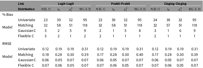
Percentage biases and RMSEs for the ATE of an endogenous right-hand-side variable, estimated on data simulated using logit links for the treatment and outcome variable, and normal, Student’s $t$ , $\unicode[STIX]{x1D712}^{2}$ and uniform distributions for the unobserved confounder, when setting the coefficient of the unobserved confounder to $-0.85$ in the treatment equation. The percentage bias is defined as the average difference between the estimator and the true parameter divided by the true parameter. The RMSE is the square root of the mean of the squared deviations of the ATE estimates from their true values. Bias tells us how well or poorly the estimator does on average in estimating the ATE, while the RMSE reflects both the bias and the precision of the estimator. For both statistics lower numbers indicate a better-performing estimator; examining both helps to diagnose whether a poorly performing estimator suffers from imprecision or bias or both. The 250 simulated datasets were used to fit Gaussian, Frank, $\text{Clayton}_{90}$ , $\text{Clayton}_{270}$ , $\text{Joe}_{90}$ , $\text{Joe}_{270}$ , $\text{Gumbel}_{90}$ and $\text{Gumbel}_{270}$ copulas with logit, probit and complementary log–log link functions for the treatment and outcome variable. The recursive bivariate model with Gaussian copula is denoted as Gaussian C and the flexible recursive bivariate model in which the copula is selected by AIC is refereed to as Flexible C.

4 Simulations

The aim of this section is to use simulations to assess the empirical effectiveness of the copula recursive bivariate model for binary outcomes. Because simulated results are of marginal interest when the data-generating process conforms to the assumptions of the authors’ preferred model and the parameters can be set to degrade the performance of its competitors, we focus mostly on simulations in which none of the models captures the correct distributional assumptions. The goal is to compare model performance under what we take to be the most likely scenario for political scientists attempting causal inference: at least one confounder is omitted, the marginal distributions and dependence structure are unknown, and the goal is to recover the best (i.e., least biased and lowest RMSE) estimate of the ATE.

In the following simulations, a binary instrument, two continuous observed confounders, one continuous unobserved confounder, a binary treatment and a binary outcome are denoted as $z_{3}$ , $z_{1}$ , $z_{4}$ , $z_{2}$ , $x$ and $y$ , respectively. We constructed the responses $y$ and $x$ using several distributions for the unobserved confounding variable $z_{2}$ (standard Normal, Student’s $t$ with four degrees of freedom, $\unicode[STIX]{x1D712}^{2}$ with one degree of freedom and uniform $[-3,3]$ ) and used logit link functions for the treatment and outcome variable, giving four simulation scenarios in total. Variable $z_{3}$ was simulated with two categories (0 and 1) with $\text{Pr}(z_{3}=1)=0.5$ . Variables $z_{1}$ and $z_{4}$ were generated from uniform distributions over $[0,1]$ . Nonlinear covariate effects between $y$ and $z_{1}$ and $z_{4}$ , and between $x$ and $z_{1}$ and $z_{4}$ were also introduced. The coefficient of the unobserved confounder $z_{2}$ was set to $-0.85$ in the treatment equation. The sample size was 1000. Each scenario was replicated 250 times. Following a reviewer’s suggestion, we conducted further simulations with different values of the coefficient of $z_{2}$ in order to assess the size of bias and RMSE in relation to the importance of the unobserved confounder. A full description of the simulations is found in the Supplementary Appendix.

Table 1 compares the bias and root mean squared error (RMSE) for the ATE from a univariate model (i.e., a recursive model that assumes uncorrelated errors and therefore adjusts only on observed covariates), genetic matching (an approach that matches on individual observed covariates using an automated search algorithm to balance covariates), a recursive bivariate model with Gaussian copula (Gaussian C in the table), and a flexible recursive bivariate model in which the preferred model is selected by AIC (this is referred to as Flexible C).Footnote ³ Note that the recursive bivariate model with Gaussian copula and probit link functions corresponds to a bivariate probit.

Given the existence of an unobserved confounder, we should expect the first two models, both of which assume selection on observables, to perform poorly, and they do: bias ranges from 23%–95% and 32%–118%, respectively, and RMSE from 0.12–0.31 and 0.17–0.40.

Moving to a standard recursive bivariate model with a Gaussian copula, we can see that simply allowing for unobserved confounders dramatically reduces both bias and RMSE relative to the models that assume selection on observables: decreases in average bias of 90% or more are not uncommon. By contrast, allowing different marginal distributions across recursive bivariate models with a Gaussian copula does virtually nothing to decrease bias or improve RMSE.Footnote ⁴

Use of the flexible copula model improves our estimates even further. On the whole, use of the flexible copula model results in a reduction of the bias of the ATE relative to a standard recursive model with the same marginal distributions. This difference is greatest in the case of non-Gaussian errors, where the performance of the traditional recursive bivariate model worsens significantly whereas that of the flexible copula model remains reasonably consistent. In these cases, reduction of the bias of the ATE averages about 50%. Differences in ATE estimates between Gaussian and flexible copula models were generally statistically significant at $p=0.05$ .Footnote ⁵

Although these conclusions are valid for the simulation settings considered here, it cannot be determined a priori whether relaxing the distributional assumptions will lead to dramatically different estimated ATE as the true structure in the data is unknown. However, these results do suggest that there are a variety of scenarios in which incorrect distributional assumptions lead to biased results and in which a flexible recursive bivariate model can substantially mitigate this bias.

In order to illustrate the utility of the flexible recursive bivariate model in practice, we now turn to an example from the literature on international institutions: the debate over the impact of ratification of Article VIII of the International Monetary Fund’s Articles of Agreement on compliance.

5 The Impact of International Institutions

To highlight the utility of these models in political science, we have reexamined the debate over Article VIII ratification and compliance that was first explored by Simmons (Reference Simmons2000). This is an ideal example to examine for two reasons: its structure—endogenous ratification as a determinant of compliance—is quite typical of studies of international institutions (as well as for regimes, international organizations, and state behavior more generally), and in the course of the debate the original study’s conclusions have been reexamined using both joint likelihood methods (von Stein Reference von Stein2005) and matching methods (Simmons and Hopkins Reference Simmons and Hopkins2005).

At issue is the impact of treaty commitment on compliance. Article VIII stipulates that signatories must keep their current accounts free from restrictions. Individual governments may be tempted to restrict current accounts to realize short-term gains, such as developmental objectives or the easing of balance-of-payment difficulties, but doing so is inimical to the longer-term collective goal of open foreign exchange. Simmons chose to explore Article VIII because its effects are uncontaminated by external considerations: commitment to Article VIII is voluntary, and there are neither positive incentives to commit nor sanctions for noncompliance (Simmons Reference Simmons2000, 820). The interesting question for students of institutions is whether, and to what extent, formal commitment to Article VIII increases compliance by reducing the probability that a state will impose current-accounts restrictions.

Clearly, Article VIII ratification cannot be viewed as a random “treatment.” Simmons (Reference Simmons2000) recognizes the endogeneity of Article VIII status but, citing the absence of a good instrument (fn. 25), utilizes a logit model on cross-sectional time-series data. In doing so, she leverages the insight of Beck, Katz and Tucker (Reference Beck, Katz and Tucker1998), who pointed out that annual cross-series time-section data are equivalent to grouped duration data. Following their recommendations, she accounts for temporal dependency using two time splines of a measure of the time elapsed since the state’s last currency restriction. She finds that Article VIII commitments increase the probability of compliance by up to 27% in the first year after commitment, though the effect subsequently diminishes and fades to insignificance after about five years.

In a follow-up study, von Stein (Reference von Stein2005) argues that screening effects, rather than constraining effects, could easily account for Simmons’ results—that is, that states preferentially opt in to treaties with which they are already willing to comply. She also underscores the endogeneity of Article VIII status and argues that unmeasured confounders—variables that have an impact both on commitment and compliance—are potentially problematic for Simmons’ results. Von Stein points to Vreeland (Reference Vreeland2003, 5–8), who lists two examples of unobservables that could confound the impact of IMF programs on outcomes: “political will,” or the resolve of countries that are determined both to make a commitment in the first place and, subsequently, to uphold it; and trust in government, which provides the societal support necessary both to permit a government to make an IMF commitment and to weather its possible adverse repercussions.

To estimate the impact of Article VIII commitment net of these unobservables, von Stein derives an original dual-selection model based on a standard bivariate probit in which the probability of restriction is modeled separately for signatories and nonsignatories—that is, states are “selected” into either signatory or nonsignatory status. Like Simmons, von Stein uses time splines to account for temporal dependence (fn. 12). In addition, she utilizes two dummy variables in the selection equation that are equal to 1 if the state in question restricted current accounts in the present or the previous year, respectively, and equal to 0 otherwise, to ensure that the coefficient estimates are “based on the variables’ effects before and when states sign, but not after” (618).

Based on her results, von Stein concludes that Simmons’ estimate of the impact of treaty commitment on compliance is overly optimistic—roughly double what it should be. Moreover, this reduced effect can no longer be distinguished from zero at standard levels of statistical significance. Von Stein also finds a statistically significant correlation between the error terms of the selection and outcome equations for signatories, implying that the unmeasured confounders that produce commitment also produce compliance. Intriguingly, the correlation of the error terms of the equations for nonsignatories is not statistically significant, implying that the converse is not true.

Simmons and Hopkins (Reference Simmons and Hopkins2005) reply by pointing to the well-known frailty of “Heckman-style” models in the face of violations of their distributional assumptions (624–627). Moreover, they point out that the dummy variables used by von Stein to restrict the selection equation to the precommitment period are problematic, both in that they induce quasi-perfect separation and in that they account for almost all of the difference between von Stein’s estimate of the effect of treaty commitment and Simmons’ original estimate (626).

Simmons and Hopkins’ solution to the larger selection-on-unobservables issue involves theorizing and measuring the unobserved confounders—specifically, using capital account openness and GATT/WTO membership as proxies for unobserved political will—and then using matching to calculate the ATE of commitment to Article VIII. While their matching-based estimate of the ATE corresponds well with the estimate from Simmons’ original paper, they admit in the final paragraph that,

While this statement is true, it does raise important questions. How can we be reasonably certain that all unmeasured confounders have been accounted for? If unobserved confounders remain, to what extent does their omission bias the matching-based estimate of the ATE? And how can we obtain separate estimates of the screening and constraining effects of Article VIII commitment, rather than the impact of commitment net of both?

Rather than attempting to address these questions within the context of matching, we instead address Simmons and Hopkins’ concerns about the impact of rigid functional-form assumptions in joint likelihood models by relaxing those assumptions.

5.1 Analysis and results

To explore the screening and constraining impacts of Article VIII, we utilized a flexible recursive bivariate binary model on the commitment and compliance variables from Simmons and Hopkins’ reanalysis. We use the Ali–Mikhail–Haq (AMH) copula with two logit marginals: this model produced the lowest AIC score of any marginal-copula combination,Footnote ⁶ and a Clarke test (Clarke Reference Clarke2007) indicated that it was to be preferred over the closest contender, a model with logit marginals and a Gaussian copula.Footnote ⁷ We account for temporal dependence with smoothing splines to capture the nonlinear relationships between both years of IMF membership and commitment and years since last restriction and compliance. The exclusion restriction is clearly satisfied: universality and regional norms, in particular, are unlikely to produce currency restriction except via Article VIII commitment.

Table 2.

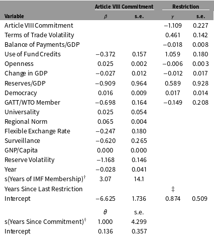
Determinants of Article VIII ratification and compliance.

$\dagger$ Reported spline values are effective degrees of freedom and Chi-square, respectively.

$\ddagger$ Ten coefficients (for dummy variables for one year, two years, …, 10 years) omitted to save space. Coefficients ranged from $-$ 3.964 to $-$ 5.436; all were significant at $p<0.01$ . $n=2,288$ , average  $\unicode[STIX]{x1D703}=-0.024$ ( $-$ 0.457, 0.635), total edf  $=$  39.1.

The results of the analysis, displayed in Table 2, comport very well with theoretical expectations and findings from Simmons’ original study. Of more than 20 coefficients, only one—Change in GDP, an economic control in the Commitment equation—both changes sign and becomes statistically significant. Two variables in the Restriction equation, Change in GDP and Reserves/GDP, retain their predicted sign but become statistically insignificant, while two others—Reserve Volatility in the Commitment equation and Openness in the Restriction equation—retain their predicted sign but become statistically significant. Leaving aside the impact of Article VIII commitment on restriction for the moment, then, the remaining theoretical conclusions regarding the determinants of commitment and restriction are largely similar to those in the original study.

The third equation, at bottom, models $\unicode[STIX]{x1D703}$ , the parameter that captures the strength of the association of the errors between the two equations, as a function of years since (or, if negative, prior to) commitment to Article VIII. The goal is to capture either transient shocks around the time of signing—the temporary rise of an unusually sympathetic government, say, or the presence of propitious short-term conditions—or longer-term internalization of (or disenchantment with) the norms of the treaty. The results show a weakly positive association, and a plot of the spline function (not shown) shows a linear relationship.

Figure 2.

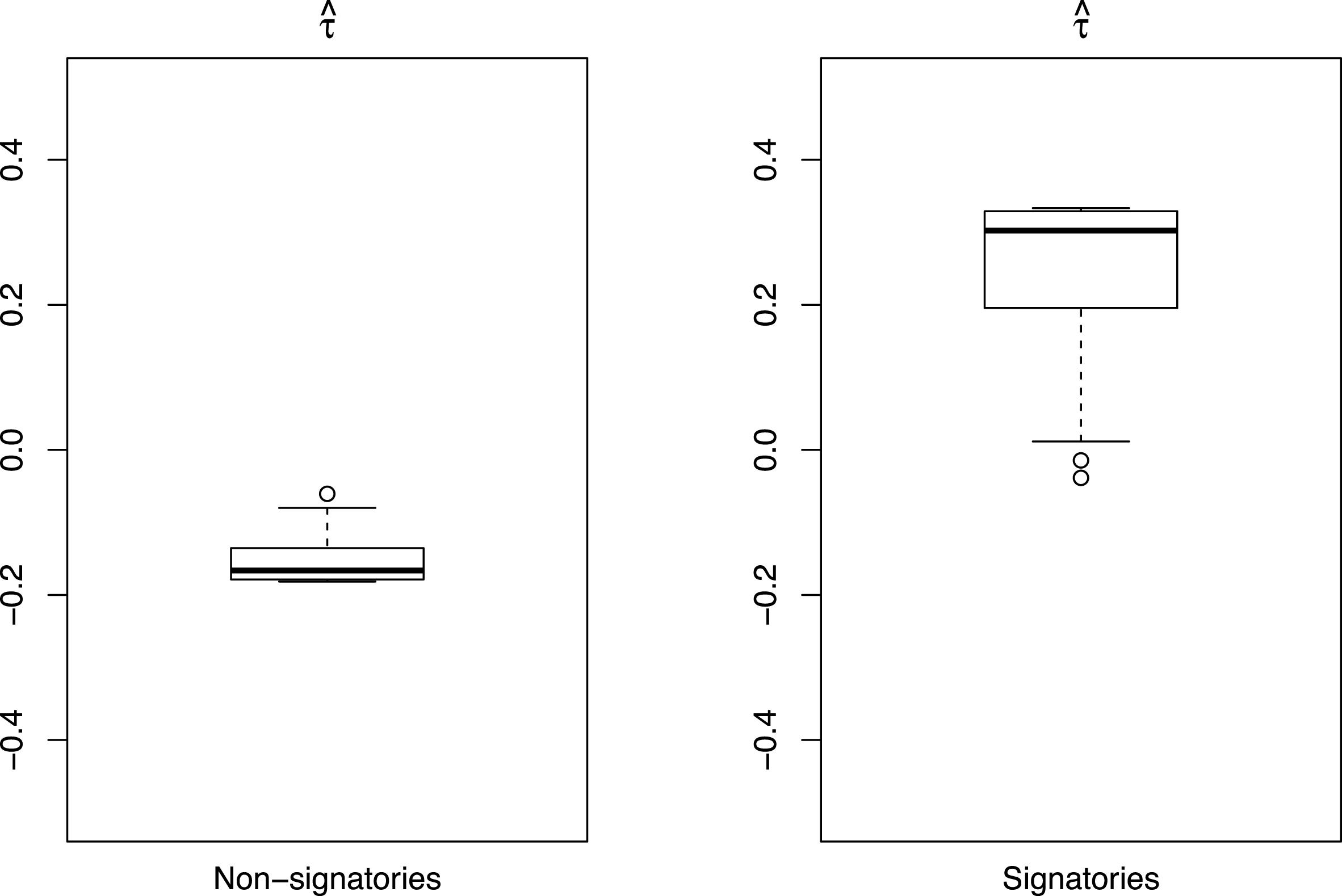
Estimated values of Kendall’s $\unicode[STIX]{x1D70F}$ , the measure that reflects the strength of the association between the error terms of the commitment and restriction equations, for nonsignatories and signatories. Note that the Kendall’s $\unicode[STIX]{x1D70F}$ is a function of $\unicode[STIX]{x1D703}$ and produces values in the customary range $[-1,1]$ .

As Figure 2 demonstrates, the impact of unobserved confounders varies markedly between nonsignatories and signatories. As we might expect, unobserved “shocks” were negatively associated among nonsignatories, indicating that unobserved confounders that decreased (increased) the propensity to commit also increased (decreased) the probability of currency restriction. The asymmetric tail of the AMH copula indicates that this association is especially strong. Among signatories, we see a positive association among shocks: unobserved confounders that increased the propensity to commit increased the probability of currency restriction. This result suggests that some unmodeled variable (changes in government, perhaps) decreases postcommitment enthusiasm for compliance. The fact that unobserved confounders pull in opposite directions across the two groups of states is one of the conclusions that would have been missed by a less flexible standard recursive bivariate probit model. As we will soon see, it turns out to be an important one.

Using the chosen model, we calculate the ATE of Article VIII commitment, given by

$$\begin{eqnarray}\frac{1}{n}\mathop{\sum }_{i=1}^{n}\unicode[STIX]{x1D6EC}(\hat{\unicode[STIX]{x1D6FD}}_{1}+\hat{f}_{1}(\{\mathbf{X}\}_{[-x_{1}],i}))-\unicode[STIX]{x1D6EC}(\hat{f}_{1}(\{\mathbf{X}\}_{[-x_{1}],i})),\end{eqnarray}$$

where $\unicode[STIX]{x1D6EC}$ is the cumulative distribution function of a standard logistic distribution. This formula captures the difference between the probability of restriction given Article VIII commitment (the first term) and the probability of restriction given no Article VIII commitment (the second term) for each observation $i$ , summed across all $n$ observations. We generate a 95% confidence interval for the ATE via posterior simulation.

The screening hypothesis, in which the states that sign are states for which compliance involves very little change in behavior, implies that there is a systematic difference in the ATE between signatories and nonsignatories. To the extent that it holds, we should expect to see that the ATE among nonsignatories is systematically greater than it is among signatories, indicating that they would have to change their behavior more radically than would signatories in order to comply. The compliance hypothesis, by contrast, suggests that the ATE for signatories should be positive and statistically significant.

The ATE for signatories is found to be $-0.059$ . That is, the average effect of signing Article VIII is to reduce the risk of current account restriction (increase the probability of compliance) by 5.9%. These results suggest that signing on to Article VIII has a significant, if modest, impact on state behavior. 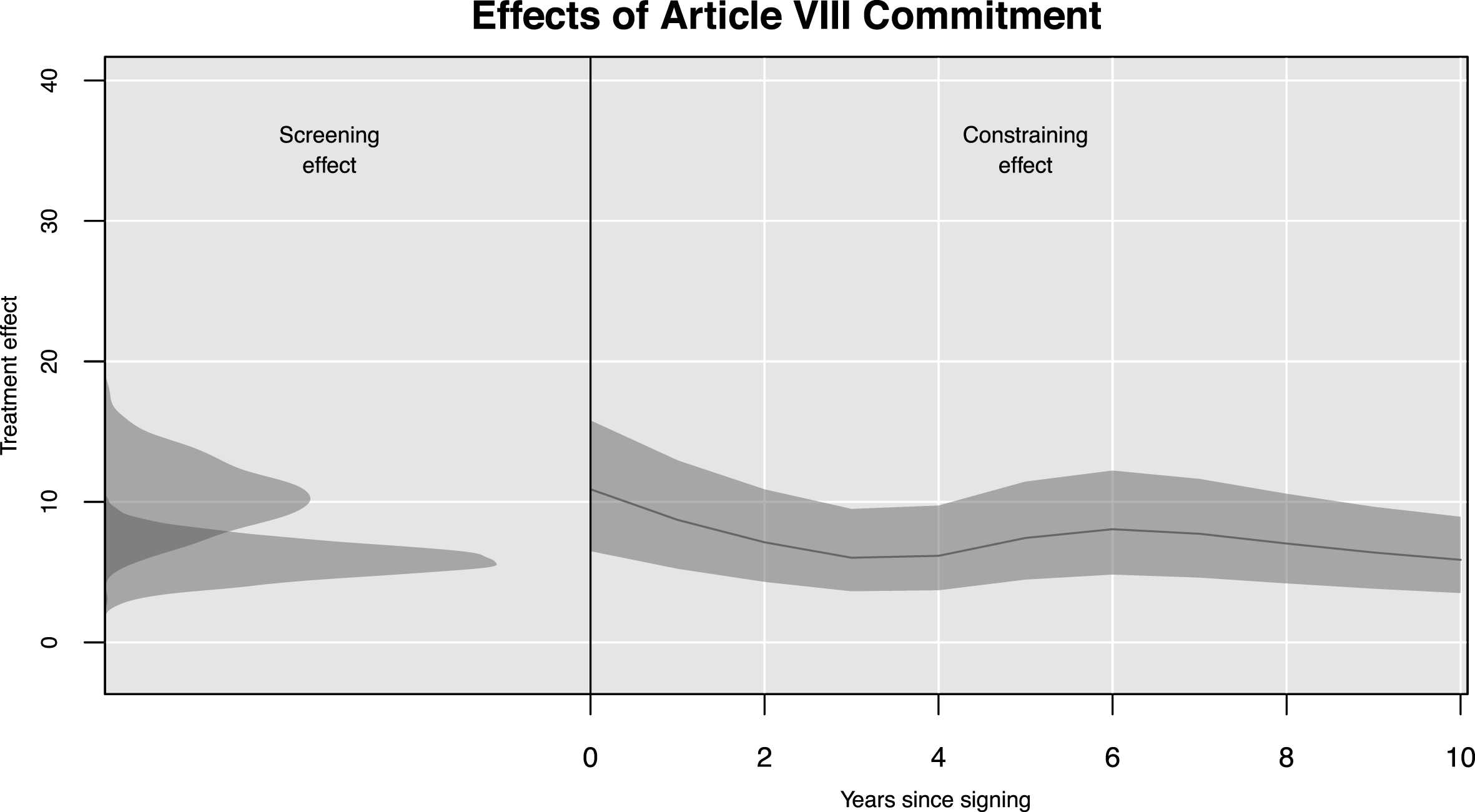For nonsignatories, the model produces an ATE of $-0.105$ —nearly twice that of signatories.Footnote ⁸ This difference, illustrated on the left of Figure 3, provides strong evidence of a screening effect. The states that sign are fundamentally different from the states that do not: in the counterfactual world in which these nonsignatories were to sign, doing so would require a much more substantial change in behavior. In short, these results support von Stein’s contention that Article VIII screens states that have a higher cost of compliance.

Figure 3.

Average treatment effect of commitment to Article VIII, for signatories and nonsignatories. The Y-axis represents the ATE measured in terms of percentage change in the probability of compliance. For the screening effect, the shaded areas represent the distributions of treatment effects for signatories (bottom) and nonsignatories (top), while for the constraining effect the shaded area represents 95% confidence intervals.

To explore the impact of commitment on compliance over time, we disaggregate the ATE by year since signing (Figure 3, right-hand graph). As one might expect, the effect of the treaty is not constant over time. When unobservables are properly accounted for, the effect of Article VIII commitment shrinks to about a 10% increase in the probability of restriction immediately after signing.

What is much more striking is the fact that the ATE remains relatively constant, between 5% and 10%, for an entire decade after signing. While the results of Simmons’ original model (2000, 831) suggested that the impact of signing drops below 5% after three years and fades to substantive and statistical insignificance after five years, our results indicate a much more robust and lasting effect—welcome news for students of international institutions.

The impact of unobserved confounders is worth a brief note as well. By comparing the ATE estimates from our final model with those of a univariate model—i.e., a model that assumes no association between error terms—we can see that unobserved confounders have little impact on the ATE for signatories: the increase in the probability of compliance associated with commitment was 5.9% in the full model and 5.7% in the univariate model. Unobserved confounders had a much more substantial impact on the ATE for nonsignatories; however: the ATE for nonsignatories was 10.5% in the full model but only 5.7% in the univariate model. Given that Simmons and Hopkins went to a substantial amount of effort to include as many causes of compliance as possible but paid less theoretical attention to variables that might produce a screening effect, while von Stein relied on the error terms in her model to capture screening effects, this result makes quite a bit of sense.

In all, the results suggest that both Simmons and von Stein were correct. Simmons was correct about the main finding: commitment to Article VIII does increase compliance, and its impact is far more lasting than previously thought. Von Stein was correct about the magnitude of the ATE (if not its statistical significance or duration) and about the existence both of significant screening effects and of important unobserved confounders.