1. Introduction
Metamaterials are engineered materials that have been developed to alter the standard properties of wave propagation such as dispersion, refraction or diffraction; metamaterials are usually arranged in periodic patterns, at scales that are smaller than the wavelengths of the phenomena they influence. The simplest effect is that, when waves propagate in a periodic structure, the dispersion relation displays band structures with forbidden frequency regions, called band gaps. This effect, for example, can be obtained in biatomic materials (Hussein, Leamy & Ruzzene Reference Hussein, Leamy and Ruzzene2014). The concept of metamaterials was first developed in the field of optics (Pendry Reference Pendry2001), and later extended to phononic crystals and elastic waves (Hussein et al. Reference Hussein, Leamy and Ruzzene2014). In the field of surface gravity waves, the ability to control and manipulate wave properties has been an area of significant interest due to its implications for a variety of applications; several studies have made noteworthy contributions to this domain, see for example Hu et al. (Reference Hu, Shen, Liu, Fu and Zi2003, Reference Hu, Chan, Ho and Zi2011), Han L. & Chen (Reference Han, Chen and Chen2022), Han et al. (Reference Han, Duan, Duan, Zhu, Chen, Yin and Chen2024), Kucher et al. (Reference Kucher, Koźluk, Petitjeans, Maurel and Pagneux2023), Huang et al. (Reference Huang, Dai, Yuan and Jia2024), Euvé et al. (Reference Euvé, Pham, Petitjeans, Pagneux and Maurel2024), Anglart et al. (Reference Anglart, Maurel, Petitjeans and Pagneux2024), Koukouraki et al. (Reference Koukouraki, Petitjeans, Maurel and Pagneux2025), Euvé et al. (Reference Euvé, Pham, Petitjeans, Pagneux and Maurel2024a ,Reference Euvé, Pham, Petitjeans, Pagneux and Maurel b ) and Euvé (Reference Euvé2023). Moreover, during the 1980s and 1990s, significant research efforts were dedicated to understanding the interaction between gravity waves and macroscopic periodic structures, such as a sinusoidal seabed with dimensions comparable to the wavelength of the waves. Notable studies, including those in Davies & Heathershaw (Reference Davies and Heathershaw1984) and Hara & Mei (Reference Hara and Mei1987) provided valuable insights into this complex phenomenon. These investigations revealed the presence of a resonant mechanism, referred to as Bragg scattering, which occurs when the wavelength of the periodic seabed undulations is precisely half that of the surface gravity waves. When this resonance occurs, waves are reflected by the seabed. Reflection can also take place in the presence of the phenomenon of local resonance. Local resonators are usually engineered to have specific natural frequencies; when waves pass through the material and their frequency matches the natural frequency of the resonators, the resonators vibrate intensely. This resonance causes strong interactions with the wave, leading, in some cases, to its reflection. With surface gravity waves, Evans & Linton (Reference Evans and Linton1989) have shown that a submerged body, which can move subject to a restoring force, can totally reflect an incident wave of a particular frequency. This phenomenon of local resonance has also been studied in point absorber devices, see Evans (Reference Evans1976), which are designed to convert energy from surface waves. In this paper, we focus on the local resonance resulting from the interaction between surface gravity waves and a number of submerged reversed pendula, displayed in a periodic array.
In general, the interaction of ocean waves with structures is a long standing problem in fluid mechanics (Dean & Dalrymple Reference Dean and Dalrymple1991); a theoretical approach based on the direct use of the equations of motion, even in their simplified version, is not always feasible, especially when geometries are not simple and bodies are moving subject to hydrodynamic forces. In this context, numerical approaches offer a valid alternative despite the overall system complexity. With respect to standard computations in fluid mechanics, the main complication arises because of the presence of a free surface and a moving solid boundary which substantially increases the difficulty of the numerical treatment. Concerning force evaluation, some studies in the literature assume irrotational and inviscid flow so that the potential flow equations can be solved, and forces are limited to the pressure contribution (Heikkinen, Lampinen & Böling Reference Heikkinen, Lampinen and Böling2013; Abbasnia & Soares Reference Abbasnia and Soares2018). However, when the goal is to study the overall effect of wave attenuation and the energy dissipated in the bulk of the fluid, vorticity and viscosity cannot be neglected, and the full Navier–Stokes equations need to be solved: recent works (Jin et al. Reference Jin, Patton and Guo2018; Xu et al. Reference Xu, Li, Xia, Chen and Gao2019) have provided evidence that viscosity plays an important role, especially close to resonant conditions. To this end, fully resolved numerical simulations of a free surface flow interacting with a structure represents a powerful tool that can provide a detailed representation of the flow field and fluid–structure interaction.
We perform numerical simulations of surface gravity waves propagating between water and air with submerged pendula in a two-dimensional framework; therefore, strictly speaking, our waves are characterised by infinitely long crests and the oscillators are cylinders whose axes are parallel to the crests. The choice of cylinders as resonators is to minimise shape-related effects, which are of secondary interest here, and because they are the two-dimensional equivalent of spherical resonators in three dimensions, the latter allowing an isotropic geometry. We solve the full Navier–Stokes system of equations coupled with the volume of fluid (VoF) method for the interface tracking and the immersed boundary method (IBM) for the fluid–structure interaction. The cylinders undergo the hydrodynamic forces (pressure and viscous stress) of the wave motion and an elastic force, gravity, which tends to restore the system back to the equilibrium position (being lighter than the surrounding fluid). The analysis has been conducted for a variable number of resonators per wavelength and varying their natural frequency. Differently from De Vita et al. (Reference De Vita, De Lillo, Bosia and Onorato2021a ), here, we employ a numerical wave tank which allows us to reach a steady-state solution, in terms of average system energy, and evaluate the resonator effects both upstream and downstream. Additionally, the horizontal and vertical motions of the resonators are accounted for, while in De Vita et al. (Reference De Vita, De Lillo, Bosia and Onorato2021a ) only the horizontal motion was considered.
It is worth mentioning that the system we are considering is similar to systems for wave energy conversion, with a rich literature ranging from point absorbers (Li & Yu Reference Li and Yu2012; Zurkinden et al. Reference Zurkinden, Ferri, Beatty, Kofoed and Kramer2014; Xu et al. Reference Xu, Li, Xia, Chen and Gao2019) to a full modelling of the solid structure (Heikkinen et al. Reference Heikkinen, Lampinen and Böling2013; Anbarsooz, Passandideh-Fard & Moghiman Reference Anbarsooz, Passandideh-Fard and Moghiman2014) and also to tethered submerged floaters for coastal protection which have been recently investigated under the project METAREEF (https://www.waveabsorber.unito.it) by means of laboratory experiments (Lorenzo et al. Reference Lorenzo, Pezzutto, De Lillo, Ventrella, De Vita, Bosia and Onorato2023).
2. Methodology
2.1. Physical model
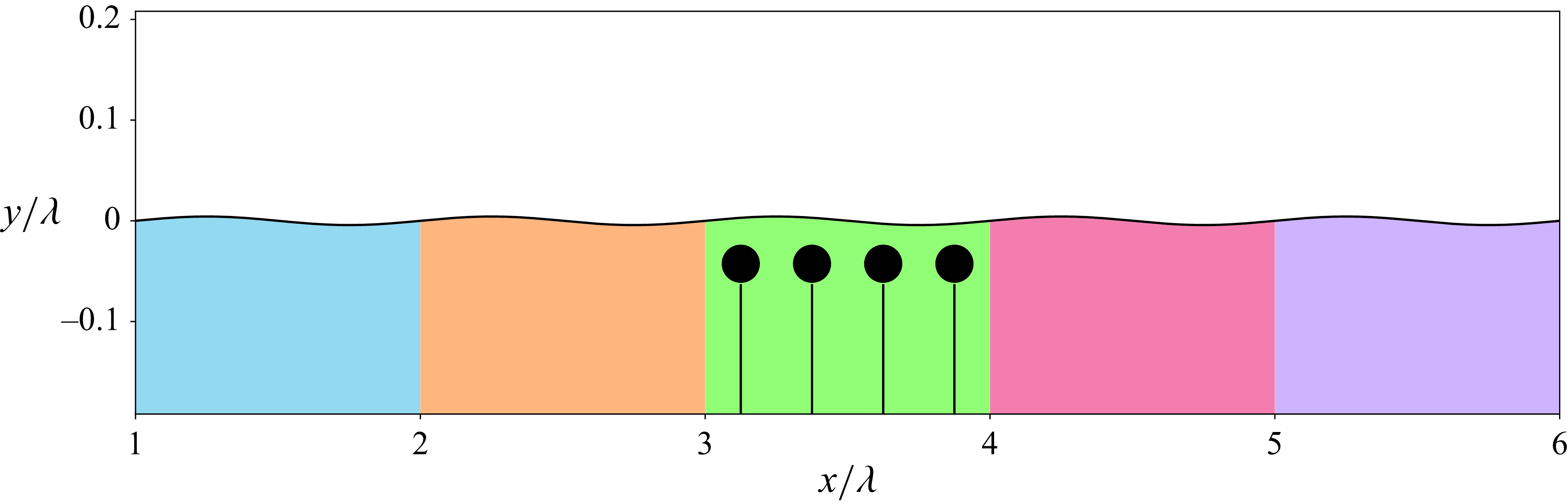
We perform numerical simulations of unidirectional monochromatic waves propagating over submerged resonators. A sketch of the set-up is reported in figure 1. The domain is two-dimensional, with
 $x$
the wave propagation direction and
 $y$
the vertical direction.
Sketch of the computational domain with five region of interest coloured as the line colours used in the following plots. Note that plot axes are not in physical scales, hence cylinders should look like ellipses. The shape has been reported as cylinder for clarity. Here,
 $\lambda$
represent a characteristic wavelength.

Surface gravity waves propagate at the interface between two immiscible fluids with constant material properties. The resonators are modelled as fully submerged cylinders, anchored to the bottom of the domain, with tensioned wires. This is true if the density of the resonator is sufficiently lower than the fluid density. Within this description, resonators can be considered as submerged reversed pendula whose motion is constrained over an arch centred at the anchoring, each resonator having one rotational degree of freedom.
The full system is governed by the Navier–Stokes equations, which describe the flow dynamics, coupled with the Newton–Euler equations, for the motion of the resonators. To model the multi-phase nature of the flow, we adopt the one-fluid formulation which considers the two-fluid system as a single one with variable material properties in space and a semi-analytical VoF technique to track in time the interface (Rosti et al. Reference Rosti, De Vita and Brandt2018); finally, the coupling between the fluid and the solid phase is modelled using a direct forcing IBM (Fadlun et al. Reference Fadlun, Verzicco, Orlandi and Mohd-Yusof2000). The full system reads
 \begin{align}&\qquad\qquad\qquad\quad \nabla \cdot \mathbf{u} = 0 ,\end{align}
 \begin{align}& \rho \frac {\partial \mathbf{u}}{\partial t} + \rho \mathbf{u}\cdot \nabla \mathbf{u} = -\nabla p + \nabla \cdot \boldsymbol{\tau } + \rho \mathbf{g} + \mathbf{f} + \mathbf{s} ,\end{align}
 \begin{align}&\qquad\qquad\quad\, \frac {\partial \mathcal{H}}{\partial t} + \mathbf{u}\cdot \nabla \mathcal{H} = 0 ,\end{align}
 \begin{align}&\qquad\qquad\qquad\quad \frac {{\mathrm{d}} \Omega _n}{{\mathrm{d}}t} = \frac {T_n}{I_n}, \end{align}
 \begin{align}&\qquad\qquad\qquad\quad \frac {{\mathrm{d}} \Theta _n}{{\mathrm{d}}t} = \Omega _n, \end{align}
with
 $\mathbf{u}(\mathbf{x},t)$
representing the fluid velocity field,
 $p(\mathbf{x},t)$
the fluid pressure field,
 $\mathcal{H}(\mathbf{x},t)$
an indicator function with value 0 in one fluid and 1 in the other,
 $\rho (\mathcal{H})$
the fluid density,
 $\boldsymbol{\tau } = (2 \unicode{x03BC} \mathbf{D})$
the viscous stress tensor,
 $\mu (\mathcal{H})$
the fluid dynamic viscosity,
 $\mathbf{D}$
the strain rate tensor, defined as
 $D_{ij} = 1/2(\partial u_i/\partial x_j + \partial u_j/\partial x_i)$
,
 $\mathbf{g}$
the gravity vector,
 $\mathbf{f}$
an external force vector used to impose the no-slip boundary condition on the solid surface by means of the IBM and
 $\mathbf{s}$
a source term used to generate and absorb waves (described in the next section). Material properties are linked to the indicator function as follows:
 \begin{align} \rho (\mathcal{H}) &= \mathcal{H} \rho _1 + (1 - \mathcal{H}) \rho _0 ,\end{align}
 \begin{align} \mu (\mathcal{H}) &= \mathcal{H} \mu _1 + (1 - \mathcal{H}) \mu _0, \end{align}
with
 $\rho _1$
and
 $\mu _1$
the density and dynamic viscosity of one fluid, i.e. where
 $\mathcal{H} = 1$
and
 $\rho _0$
and
 $\mu _0$
are the density and dynamic viscosity of the other fluid, i.e. where
 $\mathcal{H} = 0$
. Upper case variables represent solid phase variables, with
 $\Omega _n$
the angular velocity of solid body
 $n$
,
 $\Theta _n$
its centre of mass rotation and
 $I_n = M_n l_n^2$
its moment of inertia, with
 $M_n$
the resonator mass (per unit width) and
 $l_n$
the distance from its centre of mass and the anchoring point. The torque
 $\mathbf{T}_n$
around the anchoring on resonator
 $n$
is obtained by summing weight
 $\mathbf{W}_n = M_n \mathbf{g}$
and the hydrodynamic loads
 $\mathbf{F}_n$
 \begin{equation} \mathbf{T}_n = \mathbf{r}_n \times \left (\mathbf{W}_n + \mathbf{F}_n\right ), \quad \mathbf{F}_n = \int _{S_n} \left (-p \mathbf{n} + \boldsymbol{\tau }\cdot \mathbf{n} \right )\, {\mathrm{d}}S ,\end{equation}
with
 $\mathbf{r}_n$
the position vector of the centre of mass of the resonator
 $n$
with respect to its anchoring point i.e. the distance vector between the resonator centre of mass and the fixed location of its anchoring point. Note that, since gravity is included on the right-hand side of the momentum equation (2.2), the pressure field
 $p$
contains the hydrostatic pressure, hence, the Archimede force contribution is already included in
 $\mathbf{F}$
. The Navier–Stokes equations are discretised with second-order central finite differences in space, on a staggered grid, and time marching of the solution is performed via a predictor corrector method with a second-order Adams–Bashforth discretisation in time; velocity correction is obtained solving a Poisson equation for the pressure increment employing a fast direct solver; the VoF advection equation is solved using the MTHINC algorithm (Ii et al. Reference Ii, Sugiyama, Takeuchi, Takagi, Matsumoto and Xiao2012). The coupling with the solid phase is implemented with an iterative fourth-order Hamming solver since, for low density solids, explicit treatment of added mass leads to instabilities (de Tullio & Pascazio Reference de Tullio and Pascazio2016). A detailed description of the numerical solver together with validations can be found in De Vita et al. (Reference De Vita, De Lillo, Verzicco and Onorato2021b
).
2.2. Numerical setup
All simulations are performed by considering a wave of wavelength
 $\lambda = 2.345$
m and a wave amplitude
 $a = 0.01$
m which correspond to a wave steepness of
 $\epsilon = ak = 0.0268$
, with
 $k = 2\pi /\lambda$
the wavenumber; the water depth is equal to
 $h = 0.45$
m. Density and viscosity ratios are those of air and water, i.e.
 $\rho _1/\rho _0 = 1/850$
and
 $\mu _1/\mu _0 = 1.9 \times 10^{-2}$
, with
 $\rho _0 = 1000$
 $\mathrm{kg\,m}^-{^3}$
while the viscosity of the reference fluid is chosen fixing the value of the Reynolds number
 $Re = \rho _0 c \lambda /\mu _0$
to
 $10^6$
, with
 $c = \sqrt {g \lambda }$
the reference velocity. This value is approximately ten times smaller than the one corresponding to water; with this choice, the viscous dissipation is higher, but the energy transfer between the travelling wave and the resonators is reduced. However, due to the high value of the Reynolds number, we do not expect relevant effects on the results. Resonators have a radius
 $r = 0.05$
m and their centre of mass is initially located at
 $y = -0.1$
m (with the origin of the
 $y$
axis on the still water level, as sketched in figure 1). The horizontal position depends on the number of resonators: when using one resonator, its centre of mass is located at
 $x = 3.5\lambda$
; when using two resonators, they are located at
 $3.33\lambda$
and
 $3.66\lambda$
; finally, when using four resonators they are located at
 $3.125\lambda$
,
 $3.375\lambda$
,
 $3.625\lambda$
and
 $3.875\lambda$
. The density of the resonators
 $\rho _s$
is varied to change the ratio between the wave frequency and the resonator natural frequency: we use
 $\rho _s = [0.1\rho _0, 0.3\rho _0, 0.5\rho _0, 0.9\rho _0]$
. Since here we have two different time scales, one given by the angular wave frequency (Dean & Dalrymple Reference Dean and Dalrymple1991)
 \begin{equation} \omega _0 = \sqrt {g k \tanh {(k h)}}, \end{equation}
and a second time scale given by the resonator angular frequency
 \begin{equation} \omega _s = \sqrt {\frac {g(\rho _0 - \rho _s)}{l(\rho _s + \rho _0)}}, \end{equation}
with
 $l$
the distance between the resonator centre of mass and the anchoring. To characterise our system, we introduce the non-dimensional frequency ratio
 $\Lambda = \omega _s/\omega _0$
, which in our simulations has values
 $\Lambda = [1.02, 0.83, 0.65, 0.34]$
. To relate the set-up with classical non-dimensional scaling for flow around a cylinder, the Reynolds number based on the cylinder diameter and speed
 $Re_p = \rho _0 V d / \mu _0$
maximum value in our simulations ranges between 400 and 500.
To simulate steady-state travelling waves, we adopt a modified relaxation zone method with pressure gradient forcing (De Vita et al. Reference De Vita, Di Mascio and Onorato2022). The full computational domain has size
 $8\lambda$
in the
 $x$
direction and size
 $\lambda$
in the
 $y$
direction, while the propagation domain ranges from
 $x = \lambda$
to
 $x = 6\lambda$
, with the first wavelength used to force the propagating wave and the last two wavelengths for absorption. Relaxation zone methods are based on relaxing the solution, at each time step, to a given analytical solution as
 \begin{equation} \Phi (\tilde {x},t) = \gamma (\tilde {x})\Phi (\tilde {x},t)_{computed} + (1-\gamma (\tilde {x}))\Phi (\tilde {x},t)_{analytical}, \end{equation}
with
 $\Phi$
a generic field,
 $\tilde {x} = [0,1]$
a non–dimensional coordinate and
 $\gamma (\tilde {x})$
a weight function of the form (Chen, Kelly & Zang Reference Chen, Kelly and Zang2019)
 \begin{equation} \gamma (\tilde {x}) = 1 - \frac {e^{\tilde {x}^{3.5}} - 1}{e^1 - 1}. \end{equation}
In the generation zone, (
 $x \leqslant \lambda$
), the VoF field is relaxed via equation (2.11) to the analytical solution and, in the absorption region (
 $x \gt 6\lambda$
), both the VoF and velocity fields are relaxed to still water; the source term
 $\mathbf{s}$
in the momentum conservation equation is defined as
 \begin{align} \mathbf{s}=\begin{cases} -(1 - \gamma ({\tilde {x}}))\nabla p_{analytical} & \text{if $\tilde {x} \leqslant 1$},\\ 0 & \text{otherwise}, \end{cases} \end{align}
with
 $\tilde {x} = 1 - x/\lambda$
and
 $\nabla p_{analytical}$
the gradient of the pressure obtained from a second-order Stokes expansion (Dean & Dalrymple Reference Dean and Dalrymple1991).
Grid convergence study: comparison of fluid kinetic energy and total energy dissipation with the three adopted computational grids.

Since we have a propagation domain of size
 $5\lambda$
, we divide the domain into five regions, with resonators located always in the third one, to evaluate the mechanical energy in each of the regions. The computational domain is discretised with 10 240
 $\times$
512 grid cells, corresponding to 1280 grid cells per wavelength and approximately 54 cells per resonator diameter; the time step adopted for the simulations is approximately
 $\Delta t = 10^{-4}$
s. The choice of the computational grid was made after a grid convergence analysis. The case with one resonator with density ratio 0.1 was simulated with two additional computational grids, a coarser one of size 7680
 $\times$
384 and a finer one of size 12 800
 $\times$
640; figure 2 reports the comparison of the time history of the fluid kinetic energy and total fluid dissipation
 $\mathcal{D}$
(as defined in § 3.3), showing that the adopted computational grid is reasonably close to the finer one.
3. Results
We start our analysis describing the general system behaviour. A sinusoidal wave is generated at the left side of the domain and propagates in the positive
 $x$
direction. After an initial transient, steady propagation is reached over the whole domain and, in the absence of resonators, each of the five regions behaves identically. When resonators are located in the middle of the domain, a portion of the wave energy is transferred to each cylinder: this energy is partially used to sustain the oscillatory motion and the remaining part is transferred back to the fluid. That is, a portion of the mechanical wave energy will be reflected back (in the negative
 $x$
direction), another portion will be dissipated in the central region and the last portion will be transferred downstream of the resonators. Two movies are available as supplementary materials for the case with four resonators,
 $\Lambda = 0.65$
(Movie 1) and
 $\Lambda = 1.02$
(Movie 2).
(a,b,c): time evolution of surface elevation at first probe for different numbers of cylinders
 $n$
and frequency ratios
 $\Lambda$
: each row corresponds to a different value of
 $n$
. (d,e,f): wave amplitude spectrum as a function of non-dimensional frequency. Vertical dashed black lines represent the frequency corresponding to Bragg scattering.

(a,b,c): time evolution of surface elevation at last probe for different numbers of cylinders
 $n$
and frequency ratios
 $\Lambda$
: each row corresponds to a different value of
 $n$
. (d,e,f): wave amplitude spectrum as a function of non-dimensional frequency. Vertical dashed black lines represent the frequency corresponding to Bragg scattering.

3.1. Surface elevation in time and frequency space
Since the main objective of this study is the understanding of the attenuation of the wave motion, to evaluate the effectiveness of the system, we compare surface elevation in time at two probes location, namely
 $1.5\lambda$
(region 1) and
 $5.5\lambda$
(region 5). Figures 3 and 4 show the surface elevation
 $\eta$
at the first and the last probe, with different numbers of resonators and for different values of
 $\Lambda$
. Surface elevation is made non–dimensional with the wave amplitude
 $a$
, while time is made non-dimensional with wave period
 $T = 2\pi /\omega _0$
. Up to a non-dimensional time
 $t/T \approx 6$
, which corresponds to the time a wave travelling at phase speed needs to cross the domain and reach the absorption region, the surface elevation at the first probe overlaps for all simulations conditions; after this time, solutions start to differ. Overall, differences are more pronounced close to resonance conditions, i.e.
 $\Lambda \approx 1$
, while decreasing the value of
 $\Lambda$
, the solution tends to the sinusoidal travelling wave without resonators (reported in the figures as dashed black line). Figure 3 shows that stronger reflection is obtained in resonance condition; furthermore, in figure 4 the maximum wave amplitude reduction is obtained with four resonators in the resonance condition while, even with four resonators, for
 $\Lambda = 0.65$
, the surface elevation almost overlaps with the solution obtained without resonators. In this condition, the time scale of the restoring force (the buoyancy) acting on the resonator is larger than the time scale associated with the wave, hence, resonators will follow the wave motion with little resistance.
To show the impact of the submerged resonators on wave spectrum, we evaluate the discrete Fourier transform (DFT) of the surface elevation measured via probes. The time window of the signal used for the transformation is
 $[10t/T, 20t/T]$
with a sampling interval equal to
 $300\Delta t$
. Figures 3 and 4 (right columns) show the distribution in the frequency domain of DFT coefficients modulus: high-order harmonics are present in all simulations and are more prominent in probe 1 than in probe 5. This is because the wave energy amount in probe 5 has been reduced by the presence of the resonators. Note that we observed the growth of second and higher harmonics due to nonlinearities of the equations also in the case without resonators.
When waves propagate through a periodic structure, Bragg scattering can take place. The first energy transfer between wave components for surface gravity waves is obtained considering the resonant interaction of three waves of the form
 \begin{equation} k_1 \pm k_2 \pm k_3 = 0, \quad \text{and} \quad \omega _1 \pm \omega _2 \pm \omega _3 = 0. \end{equation}
When considering the interaction of two waves (1, 2) with the structure (3),
 $k_3 = k_d$
is the wavenumber associated with cylinder spacing
 $d$
and
 $\omega _3 = 0$
. Therefore, Bragg scattering is obtained when
 $2k = k_d$
, with
 $k_1 = -k_2 = k$
(see Lorenzo et al. Reference Lorenzo, Pezzutto, De Lillo, Ventrella, De Vita, Bosia and Onorato2023). This corresponds, in our simulations, to a frequency of
 $1.31\omega _0$
for 2 cylinders and
 $1.53\omega _0$
for 4 cylinders, as indicated by black dashed vertical lines in figures 3 and 4.
3.2. Reflection coefficient
To quantify reflection in the system, we compute the reflection coefficient as the ratio between the reflected (R) and incident (I) surface elevation variance
 $\langle \eta ^2\rangle$
 \begin{equation} C_R = \frac {\langle \eta _R^2\rangle }{\langle \eta _I^2\rangle } ,\end{equation}
where the variance is computed as
 \begin{equation} \langle \eta ^2\rangle = \sum _{i=-N_x/2}^{N_x/2}\sum _{n=-N_t/2}^{N_t/2}|A_{i,n}|^2, \end{equation}
and
 $A_{i,n}$
is the coefficient of the DFT in both time and space. The Fourier transform is performed in space from
 $x = \lambda$
to
 $x = 3\lambda$
and in time from
 $t = 10T$
to
 $t = 20T$
. For every
 $i,n$
in (3.3), the term
 $|A_{i,n}|^2$
is included in the computation of the incident wave if
 $k_i\omega _n \lt 0$
, whereas to the reflected wave if
 $k_i\omega _n \gt 0$
. Values of
 $C_R$
are reported in figure 5. Maximum reflection is obtained in resonance conditions, as expected, since Bragg resonance frequencies (reported in the plot as vertical dashed bar) are not excited by the incoming wave; moreover, close to resonance, the number of resonators slightly affects reflection. On the other side, away from resonance, increasing the number of resonators leads to a reduction of the reflection and an increase of the energy dissipation.
Reflection coefficient for different values of frequency ratio
 $\Lambda$
and number of cylinders
 $n$
. Vertical dashed lines correspond to Bragg scattering frequencies.

3.3. Mechanical wave energy
We focus our analysis on wave mechanical energy evolution. We evaluate wave mechanical energy
 $E_m(t)$
as the sum of the kinetic energy
 $E_k(t)$
and potential energy
 $E_p(t)$
 \begin{equation} E_m(t) = E_k(t) + E_p(t) = \int _{\mathcal{V}} \left (\frac {1}{2} \rho _0 |\mathbf{u}(\mathbf{x},t)|^2 + \rho _0 g y \right ) {\mathrm{d}}\mathcal{V} + E_p^0, \end{equation}
where
 $\mathcal{V}$
is the fluid domain volume and
 $E_p^0$
is the still water potential energy. For the case without resonators the fluid volume
 $\mathcal{V}$
is equal to
 $\mathcal{V} = \int _{x_1}^{x_2}\int _{-h}^{\eta }{\mathrm{d}}x{\mathrm{d}}y$
, where
 $x_1$
and
 $x_2$
are the starting and ending sections of the region considered, while for the cases with resonators the solid volume must be excluded from the volume integral.
Time history of the wave mechanical energy in different regions, for different numbers of resonators and frequency ratios.

Figure 6 displays the time history of the wave mechanical energy in each region for several simulation conditions non-dimensionalised with the reference energy of a sinusoidal linear wave i.e.
 $E_m^{ref} = \rho _0 g a^2 \lambda / 2$
. In the top left panel, the case without resonators is reported: after approximately 10 wave periods, in all regions steady state is reached. The case with
 $n = 1$
and
 $\Lambda = 1.02$
is the one with stronger reflection; this is confirmed by looking at the wave mechanical energy content regions 1, 2 and 3. Moreover, the energy available downward the system is slightly reduced. When increasing the number of resonators, reflection is reduced whereas dissipation increases strongly. From figure 6 (centre right panel), we can see that, with four resonators in resonant condition, the energy transmitted across the system is approximately 20 % of the available wave mechanical energy. For the cases with
 $\Lambda = 0.65$
(bottom panels) mechanical wave energy is almost equal to that without resonators, with most of the differences taking place in region 3, which is the region where resonators are located.
Interestingly, the way the energy is transferred back from resonators to the fluid depends on the frequency ratio. In figure 7, we report the kinetic and potential contributions to wave mechanical energy in region 3 for the case without resonators and two cases with four resonators: as expected, we recover the energy equipartition in the absence of resonators with the kinetic and potential energy being half of the reference wave mechanical energy. For the case with
 $\Lambda = 0.65$
the main effect of resonators is to increase the wave potential energy with a slightly effect on kinetic energy. Instead, in resonance conditions, kinetic energy is almost doubled.
Time history of the kinetic and potential energy in region 3.

To quantify energy dissipation, we compute the instantaneous dissipation rate by viscous stresses as
 \begin{equation} \mathcal{P}(t) = \int _{\mathcal{V}} 2 \mu \left [ \left (\frac {\partial u}{\partial x}\right )^2 + \left (\frac {\partial v}{\partial y}\right )^2 + \frac {1}{2}\left (\frac {\partial u}{\partial y} + \frac {\partial v}{\partial x} \right )^2 \right ] {\mathrm{d}}\mathcal{V}, \end{equation}
from which the total amount of energy dissipated from
 $t= 0$
to time
 $t$
can be computed as
 $\mathcal{D}(t) = \int _0^t \mathcal{P} {\mathrm{d}}t$
.
Time history of the energy dissipation rate
 $\mathcal{P}$
in different regions.

In figure 8, we report the instantaneous dissipation rate
 $\mathcal{P}(t)$
, made non-dimensional with the reference energy
 $E_m^{ref}$
and the wave period
 $T$
,
 $\mathcal{P}^{ref}=E_m^{ref}/T$
. Most of the dissipation takes place in the region where resonators are placed due to the velocity gradient generated at the solid surface and, as expected, the maximum of the dissipation is reached in resonance conditions in which, with four resonators, the instantaneous dissipation reaches value of approximately 30 % of the reference value. The average dissipation rate
 $\langle \mathcal{P}\rangle$
from
 $t = 10T$
to
 $t = 20T$
for region 3 (where the system is located) is reported in figure 9 for all cases. While dissipation increases almost linearly with the number of resonators, the dependency from the frequency ratio is more complex. There is a minimum of dissipation about
 $\Lambda = 0.34$
, which is consistent with previous results reported for horizontal resonators (De Vita et al. Reference De Vita, De Lillo, Bosia and Onorato2021a
). For this condition, resonators follow the wave motion minimising velocity gradients, which are responsible for energy dissipation. To quantify this effect, we evaluate the velocity difference between the resonator centre of mass velocity and the local fluid velocity evaluated on the free surface at same
 $x$
location,
 $\Delta \mathbf{U}(t) = \mathbf{u}(x = X(t), y = \eta (X(t), t), t) - \mathbf{V}(t)$
, with
 $X(t)$
the horizontal coordinate of the resonator centre of mass and
 $\mathbf{V}$
its velocity. The velocity difference, normalised with phase speed, is reported in figure 9 (right panel) for two different values of frequency ratio. It is clear that in resonance conditions there is a strong horizontal velocity gradient between the resonator and the local fluid velocity, enhancing viscous dissipation.
(a) Average dissipation rate
 $\langle \mathcal{P}\rangle$
as a function of the number of cylinders
 $n$
and the frequency ratio
 $\Lambda$
; (b) time history of the velocity difference for different values of the frequency ratio
 $\Lambda$
.

Resonator centre of mass motion. (a–c) Time history of resonator centre of mass horizontal position: (a,d,g,
 $n=1$
) and different
 $\Lambda$
; (b,e,h,
 $n = 4$
) and
 $\Lambda = 1.02$
; (c,f,i,
 $n = 4$
) and
 $\Lambda = 0.65$
(
 $R$
corresponds to the resonator’s number). (d–f) Modulus of DFT coefficients; dashed black line represent the first Bragg scattering frequency. (g–i) maximum amplitude oscillation for
 $n=1$
as function of
 $\Lambda$
(a,d,g), for
 $n=4$
and
 $\Lambda = 1.02$
as function of resonator (b,e,h), for
 $n=4$
and
 $\Lambda = 0.65$
(c,f,i).

3.4. Resonator motion
We first consider the case of a single resonator for different values of the frequency ratio. Figure 10(a) displays the horizontal displacement of the resonator centre of mass
 $x(t) - x(t=0)$
made non-dimensional with the wave amplitude
 $a$
. The oscillation amplitude ranges from about the wave amplitude for
 $\Lambda = 0.34$
up to approximately five times the wave amplitude close to resonance conditions, whereas the oscillation frequency is approximately the same, with a small shift in the phase. Looking at the DFT coefficient amplitude (figure 10
d–f), we can identify small higher-order harmonics and also peaks corresponding to the resonator natural frequency
 $\omega _s$
. When considering four resonators (figure 10
b,e,h,c,f,i), there is a clear amplitude reduction from the first to the last resonator when the frequency ratio is
 $\Lambda = 1.02$
, with the last one having an oscillation amplitude half of that of the first resonator. On the other side, when
 $\Lambda = 0.65$
, all resonators oscillate with same amplitude and phase with a phase shift related to the position in the domain, as shown in figure 10. The maximum amplitude oscillation of resonators grows almost linearly with the frequency ratio while it decays quadratically from the first resonators to the next ones, close to resonance conditions (figure 10
g–i). This aspect should be investigated, accounting also for the distance between resonators, which is not considered in this study.
Resonator mechanical energy for different frequency ratio and
 $n = 1$
.

Resonator mechanical energy for the case with
 $\Lambda = 1.02$
and
 $n = 4$
.

Mechanical energy for one single resonator and for different frequency ratios is reported in figure 11: in resonance conditions the wave can transfer up to 20 % of its energy to sustain the oscillatory motion of the resonator whereas a few per cent of the energy is transmitted away from the local resonance. On evaluating the case with more submerged pendula, as displayed in figure 12, in accordance with the results in figure 10, mechanical energy drops down from the first to the last resonator. When considering the collective behaviour, the energy transfer reaches approximately 30 % of the available wave mechanical energy.
To understand how the energy is exchanged between the fluid and the solid phase, it is helpful to evaluate the power acting on the resonator as the product of the force and velocity components of its centre of mass
 $\mathcal{P}^r_i(t) = F_i(t) V_i(t)$
. Figure 13 reports the displacement, the velocity, the force coefficient and the exchanged power for one single resonator with
 $\Lambda = 1.02$
and
 $\Lambda = 0.65$
. Force coefficients (per unit length) are evaluated as
 $C_i = 2F_i/(\rho _0 c^2 d)$
. For the case close to resonance conditions, a strong increase in the drag coefficient is found, whereas the lift coefficient (in the vertical direction) differs only for the contribution of buoyancy; in terms of solely hydrodynamic loads, the two cases exhibit a comparable coefficient. When evaluating the power, the components in the two directions display a similar trend, with a phase opposition. For the case with
 $\Lambda = 1.02$
, the peak value of the exchanged power is of the same order as the reference wave power. Interestingly, when integrating in time the instantaneous power
 $\mathcal{P}^r$
to retrieve the exchanged energy
 $\mathcal{E}_i = \int \mathcal{P}^r_i(t){\mathrm{d}}t$
, we find that the horizontal component acts as an energy input, whereas the vertical component is responsible for transfering back mechanical energy to the fluid phase, as shown in figure 14.
Comparison of centre of mass quantities for one single resonator and two values of
 $\Lambda$
. From top to bottom: displacement, velocity, force coefficient, exchanged power; (a,c,e,g)
 $x$
component, (b,d,f,h)
 $y$
component.

Comparison of exchanged energy in the two directions for one single resonator with
 $\Lambda = 1.02$
and
 $\Lambda = 0.65$
.

4. Conclusions
We have investigated the problem of local resonance in the interaction between surface gravity waves and submerged resonators via high fidelity numerical simulations. The case study is represented by submerged cylinders, lighter than the surrounding fluid, anchored at the bottom. When surface gravity waves propagate over these pendula, local resonance can take place, based on the ratio between the resonator natural frequency and the wave frequency. In order to properly describe the behaviour of the system, we have simulated the full Navier–Stokes equations for multiphase flows with fluid–structure interaction; this approach allows for a complete and detailed evaluation of hydrodynamic forces acting on the resonators and of the energy dissipation. Simulations were performed in a numerical wave tank with different values of the resonator/wave frequency ratio and different numbers of resonators. Results highlight the occurrence of strong reflection with one single resonator in local resonance and strong dissipation with four resonators. Conversely, away from resonance, waves propagate through the system with reduced reflection and dissipation. The motion of the resonators is strongly influenced by the frequency ratio: when the time scale of the restoring force is much longer than the wave period, the resonators are primarily driven by the wave orbital motion, oscillating with an amplitude comparable to the wave height. In contrast, when the two time scales are similar, the resonator motion becomes significantly amplified, leading to larger velocity gradients and increased energy dissipation. Mechanical energy is exchanged between the fluid and the resonators, with the latter primarily transferring energy back to the fluid through their vertical motion. Results underline the importance of viscous dissipation in the resonant condition, suggesting that neglecting viscosity can be a too rough approximation when the local resonance takes place.
From an applicative point of view, the mechanisms of local resonance and Bragg scattering can be used for coastal protection. It is well known that ocean waves are usually not characterised by a single frequency; therefore, a wave climate study should be conducted to analyse the typical wave periods in the region where the solution is intended to be implemented. Successively, one should adapt the frequency of oscillation of the pendula to the specific outcome of the research. The easiest way to adjust the oscillation frequency to match the most probable frequency of ocean waves in a specific location is by modifying their buoyant properties. This can be achieved by altering the material of the pendula or by adjusting the amount of water (or another substance) inside them, thereby changing their resonant frequency. Certainly, the length of the pendula directly affects the resonant frequency. However, this option may depend on the characteristics of the bathymetry where the device is to be deployed. Future studies should be aimed at determining the optimal spatial distribution of pendula to minimise the transmission coefficient across as many frequencies as possible. The objective is to combine both local resonance and Bragg reflection by positioning the pendula so that the frequencies of local resonances and Bragg scattering are adjacent, thereby creating a wide frequency gap where wave propagation is inhibited.
Supplementary movies
Supplementary movies are available at https://doi.org/10.1017/jfm.2025.10165.
Acknowledgements
The authors acknowledge the CINECA award under the ISCRA initiative (IsC88 project), for the availability of high performance computing resources and support. The authors are grateful to F. Bosia, P. Pezzutto, F. De Lillo and M. Miniaci for fruitful discussions during the early stages of the work.
Funding
M.O. was funded by Progetti di Ricerca di Interesse Nazionale (PRIN, 2020X4T57A and 2022WKRYNL), by the Simons Foundation (Award 652354) and by European Commission H2020 FET Open Boheme grant N. 863179.
Declaration of interests
The authors report no conflict of interest.