1. Introduction
The dissolution of stationary or entrapped gas bubbles in liquids is of great interest in many technological applications in biology, chemistry and the petrochemical industry. Gas bubbles may be generated as a consequence of biological or geological activities, gasification processes or chemical reactions. Study of the bubble dissolution dynamics is vital in determining the gas transfer rate between the bubbles and the surrounding liquid.
There are several studies in the literature that have addressed the fundamental process concerning the dissolution of an isolated spherical bubble. The mathematical problem essentially involves simultaneously solving for the equations of diffusion of species, interface motion and mass conservation. We highlight three main approaches.
-
(a) Quasi-stationary approximation methods (Holocher et al. Reference Holocher, Peeters, Aeschbach-Hertig, Kinzelbach and Kipfer2003; Shim et al. Reference Shim, Wan, Hilgenfeldt, Panchal and Stone2014), pioneered by Epstein & Plesset (Reference Epstein and Plesset1950) for a single-component bubble. Advection effects are neglected, and the time dependence of the bubble may be ignored in solving for the spherically symmetric concentration field. In such a case, the concentration gradient at the bubble surface has an analytical solution.
-
(b) Numerical methods, usually finite differences (Duda & Vrentas Reference Duda and Vrentas1971; Yung et al. Reference Yung, De Witt, Brockwell, McQuillen and Chai1989), in which the concentration field with spherical symmetry is solved for numerically. Advection and bubble gas compressibility effects may be freely included since the velocity field and bubble pressure may be straightforwardly obtained from the continuity and momentum equations respectively.
-
(c) Analytical solutions for single-component bubbles based on perturbation methods (Duda & Vrentas Reference Duda and Vrentas1969) or asymptotic expansions (Subramanian & Weinberg Reference Subramanian and Weinberg1981). These authors reported better agreement of their solutions with the (exact) finite-difference solutions than other quasi-stationary methods except at the longer times towards the end of the dissolution process. The impractical complexity and analytical limitations in the derivation of the solutions mean that their applicability outside this scope is, unfortunately, very limited.
The dissolution of multicomponent spherical bubbles has also been widely investigated. For example, Weinberg & Subramanian (Reference Weinberg and Subramanian1980) compared the performance of the quasi-stationary and finite-difference methods in illustrative examples regarding the dissolution of
 $\text{CO}_{2}$
and
 $\text{O}_{2}$
bubbles. Yung et al. (Reference Yung, De Witt, Brockwell, McQuillen and Chai1989) provide an extensive analysis of parameters affecting gas bubble dissolution, including the effect of having a non-soluble gas component in a multigas bubble.
However, in many real-life applications and natural environments, it is likely that bubbles will adhere or directly nucleate on solid surfaces. The no-flux boundary condition across an impermeable surface breaks the spherical symmetry of the concentration field in the surrounding liquid. This has a significant hindering effect on the rate of mass transport and consequently on the bubble dissolution rate.
The study of the dissolution of a single-component spherical bubble beneath a flat plate has been addressed by some authors. Early attempts involved rescaling the time variable in the Epstein–Plesset solution by a correction factor of
 $\ln (2)$
, taken from electrostatics (Liebermann Reference Liebermann1957) or potential theory (Wise & Houghton Reference Wise and Houghton1968). Kentish et al. (Reference Kentish, Lee, Davidson and Ashokkumar2006) confirmed that the value of this correction factor increases with the solubility of the gas, i.e. it is heavily dependent on the concentration boundary layer thickness. These authors also presented a finite-difference numerical model in fixed non-orthogonal coordinates (independent of the bubble radius size) that accounted for the boundary condition on the flat plate. Previously, Takemura, Liu & Yabe (Reference Takemura, Liu and Yabe1996) developed a more complex finite-difference numerical model, even including the effect of advection by simultaneously solving the vorticity transport equation. A particular tangent–sphere coordinate system was employed. However, the computational grid had to be reconstructed at each time step to account for the change in bubble radius, which can be tedious and computationally costly.
It naturally happens that most surfaces will be hydrophobic to some extent. Provided that the Bond number is small and the liquid–gas tension overcomes the buoyancy force, it is not strange to find that adhered bubbles display a spherical cap shape, with a distinct contact surface defined by a contact angle much greater than zero. For any given bubble volume, the instantaneous spherical cap surface area of the bubble depends on the instantaneous contact angle. It is then evident that the contact line or angle dynamics of a spherical cap bubble (SCB) dictates the bubble surface area dynamics and therefore will have significant impact on the SCB dissolution rate. Consequently, they must be taken into account.
As far as we are aware, no previous studies have dealt with the dissolution (or growth) of a sessile SCB adhered to an impermeable flat surface. Thus, the main purpose of this paper is to present a simple yet effective model able to predict the dissolution (or growth) rate of an isothermal multicomponent SCB attached to a smooth flat surface in a constant-pressure environment. For the first time, the equations for the diffusion of species are coupled with a simple law for the contact angle dynamics. In addition, the wall effect is explicitly treated by (a) considering the dynamic interaction of the diffusion boundary layer with the plate and alternatively (b) a novel numerical approach.
In this work, the scenario treated by the model shall be restricted to the experimental frame, in which we explore the dissolution of
 $\text{CO}_{2}$
SCB bubbles in air-saturated water. These bubbles are deposited on two substrates of different hydrophobicities: PMMA and collagen-coated coverslip glass.
This paper is structured as follows. In § 2, the problem is formulated in a generalized fashion. The experimental procedure and results are presented in § 3. In § 4, a dissolution model based on the quasi-stationary approximation is proposed. It is immediately validated against the experimental data. An approximate analytical solution for our specific experimental scenario is then discussed in § 5, from which useful insight on the dissolution mechanism is gained. In § 6, we present a finite-difference numerical method as an alternative approach to determining mass transfer across the SCB surface, and the solutions are compared. Finally, § 7 is devoted to conclusions.
2. Problem statement
2.1. Spherical cap bubble characterization and contact line dynamics
The Bond number associated with bubbles is usually defined as
 $\mathit{Bo}={\it\rho}gR^{2}/{\it\gamma}_{lg}$
, where
 ${\it\rho}$
,
 $R$
,
 $g$
and
 ${\it\gamma}_{lg}$
denote the density of the liquid, the bubble radius, the gravitational acceleration and the liquid–gas interfacial tension respectively. Spherical cap bubbles are characterized by a
 $\mathit{Bo}$
value significantly smaller than unity. In such a case, the liquid–gas interfacial tension is strong enough to overcome buoyancy forces. Surface tension will enforce a spherical cap shape in order to minimize the surface area and hence the surface energy. For
 $\text{CO}_{2}$
bubbles in water,
 $Bo\sim 0.25$
was found to be the threshold value. Additionally, the resulting force on the triple-contact line must overcome the buoyancy force so as to prevent bubble detachment. Spherical cap geometries with extremely high contact angles are also adopted by nanobubbles during the nucleation process in solid–liquid interfaces, to later exhibit a remarkable stability against dissolution (Weijs & Lohse Reference Weijs and Lohse2013; Lohse & Zhang Reference Lohse and Zhang2015).
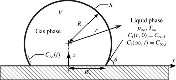
The behaviour of the SCB contact angle
 ${\it\theta}$
(see figure 1 below) in the presence of a moving contact line along a smooth homogeneous surface may be explained by a suitable contact angle hysteresis (CAH) model. It must be borne in mind that the CAH has a static component and a dynamic component (Eral, t Mannetje & Oh Reference Eral, ’t Mannetje and Oh2013). In our particular scenario of interest, i.e. the diffusion-driven dissolution of a
 $\text{CO}_{2}$
SCB in air-saturated water, the driving force is moderate. This results in slow dissolution rates and small contact line velocities, hence the quasi-static contact angle approximation may be used. The characteristic value of the capillary number (
 $\mathit{Ca}={\it\mu}{\dot{R}}_{c}/{\it\gamma}_{lg}$
, where
 ${\it\mu}$
is the dynamic viscosity of the liquid and
 ${\dot{R}}_{c}$
is the contact line velocity) was found to be small (
 $\mathit{Ca}\sim 0.005$
). Therefore, the dynamic (velocity-dependent) angle will differ from the static angle for a very small-scale hydrodynamic regime where the contact line dynamics is dominated by the viscous dissipation of the liquid. It is thus reasonable to assume that the apparent (macroscopic) angle is given by the static equilibrium angle, and that it completely describes the contact line dynamics (Snoeijer & Andreotti Reference Snoeijer and Andreotti2013).
Geometry of an SCB attached to a flat impermeable wall in a liquid–gas solution. The main system parameters concerning its diffusion-controlled dissolution or growth are also indicated.

Hong et al. (Reference Hong, Chang, Chou, Chan, Sheng and Tsao2011) recently proposed a thermodynamic model based on adhesion hysteresis able to predict the static CAH for SCBs enduring sequential changes in volume. The physical explanation for the observed CAH is that the separation energy required to make the liquid phase recede (bubble inflation characterized by an increasing SCB contact radius) is greater than the adhesion energy given by an advancing liquid phase (bubble deflation characterized by a decreasing SCB contact radius). Thus, these processes are not thermodynamically reversible, which translates into two solid–liquid interfacial tensions. Young’s equation with
 ${\it\gamma}_{sl}$
gives the liquid-advancing contact angle,
 ${\it\theta}_{a}$
, which refers to the maximum angle associated with removing gas volume from a sessile SCB. On the other hand, that with
 ${\it\gamma}_{sl}^{\prime }<{\it\gamma}_{sl}$
due to surface rearrangement yields a different liquid-receding contact angle,
 ${\it\theta}_{r}$
, which in turn corresponds to the smallest possible angle upon adding gas volume. Therefore, the contact angle is confined within the range
 ${\it\theta}_{r}\leqslant {\it\theta}\leqslant {\it\theta}_{a}$
.
When an SCB (with an intermediate
 ${\it\theta}$
) initially at equilibrium undergoes a change in volume, it is forced to adopt a new equilibrium contact angle and radius (subject to a spherical cap geometry constraint) such that the change in its free surface energy is at a minimum. This is the underlying principle of adhesion hysteresis. The contact line behaviour obtained by this approach adequately agrees with the experimentally observed fact that contact line pinning occurs when the liquid phase is advancing (bubble deflation) rather than when the liquid phase is receding.
In this work, we shall employ smooth homogeneous surfaces of mild hydrophobicity as substrates. Under these conditions, dissolving SCBs always display acute advancing angles. Consequently, only SCBs with
 ${\it\theta}\leqslant 90^{\circ }$
shall be considered.
2.2. Formulation of the problem
Consider a sessile SCB immersed in a quiescent liquid–gas solution. The SCB is adhered to an infinite flat impermeable plate described by the
 $x{-}y$
plane at
 $z=0$
, as sketched in figure 1. We restrict the bubble composition to that of
 $N$
soluble ideal gases. The flow of gas species
 $i$
in the surrounding liquid, neglecting any form of advection, is governed by the diffusion equation,
 $$\begin{eqnarray}\frac{\partial C_{i}}{\partial t}-D_{i}{\rm\nabla}^{2}C_{i}=0,\end{eqnarray}$$
where
 $C_{i}(x,y,z,t)$
denotes the molar concentration field of gas species
 $i$
, while
 $D_{i}$
refers to its diffusivity, assumed constant. Here,
 $x,y,z$
are dimensional Cartesian coordinates and
 $t$
is the time. The initial molar concentration field in the liquid is considered to be uniform and equal to
 $C_{\infty ,i}$
. Letting
 $C_{s,i}(t)$
denote the molar concentration at the interface, the boundary conditions on the concentration field are
 $$\begin{eqnarray}\left.\begin{array}{@{}l@{}}C_{i}=C_{s,i}\quad \text{on the bubble surface},\\ \displaystyle \frac{\partial C_{i}}{\partial z}=0\quad \text{on}~z=0~\text{(impermeable wall)},\\ C_{i}=C_{\infty ,i}\quad \text{at infinity}.\end{array}\!\right\}\end{eqnarray}$$
The bubble is assumed to retain its spherical cap shape throughout the whole dissolution process. Thus, the bubble dynamics may be fully described by the bubble radius
 $R(t)$
and contact angle of the liquid phase
 ${\it\theta}(t)$
, where
 ${\it\theta}\in [0,{\rm\pi}/2]$
. Accordingly, the instantaneous contact radius
 $R_{c}(t)$
, surface area
 $S(t)$
, volume
 $V(t)$
and volume rate of change
 $\dot{V}(t)$
may be written as functions of
 $R$
,
 ${\it\theta}$
and their time derivatives. From geometric considerations, one has that
 $$\begin{eqnarray}R_{c}=R\sin {\it\theta},\quad S={\rm\pi}{\it\beta}_{1}R^{2},\quad V=\frac{{\rm\pi}}{3}{\it\beta}_{2}R^{3},\quad \dot{V}={\rm\pi}R^{2}({\it\beta}_{2}{\dot{R}}-R{\it\beta}_{3}\dot{{\it\theta}}),\end{eqnarray}$$
where the dot notation
 $(\dot{~})$
is employed to denote the time derivative
 $\text{d}/\text{d}t$
. The angle-dependent functions
 ${\it\beta}_{1}({\it\theta})$
,
 ${\it\beta}_{2}({\it\theta})$
and
 ${\it\beta}_{3}({\it\theta})$
are given by
 $$\begin{eqnarray}{\it\beta}_{1}=2(1+\cos {\it\theta}),\quad {\it\beta}_{2}=(2-\cos {\it\theta})(1+\cos {\it\theta})^{2},\quad {\it\beta}_{3}=\sin ^{3}{\it\theta}.\end{eqnarray}$$
The system is at constant uniform pressure
 $p_{\infty }$
and temperature
 $T_{\infty }$
. Surface tension (
 ${\it\gamma}_{lg}$
) effects are reasonably neglected since the SCBs studied in this work had typical radii of at least a few hundred microns. It should be noted that the Laplace pressure becomes important for small radii such that
 $R\sim 2{\it\gamma}_{lg}/p_{\infty }$
, corresponding to
 $R\sim 1~{\rm\mu}\text{m}$
in standard conditions.
The bubble contents obey the equation of state for an ideal gas mixture:
 $$\begin{eqnarray}p_{\infty }V=\mathop{\sum }_{i=1}^{N}n_{i}\bar{R}T_{\infty }=n\bar{R}T_{\infty },\end{eqnarray}$$
where
 $n_{i}(t)$
and
 $n(t)$
are the number of moles of gas
 $i$
and the total moles inside the bubble respectively;
 $\bar{R}$
denotes the universal gas constant. Differentiating (2.5) with respect to time yields a differential equation for the bubble radius,
 $$\begin{eqnarray}{\dot{R}}=\frac{1}{{\rm\pi}R^{2}{\it\beta}_{2}}\frac{\bar{R}T_{\infty }}{p_{\infty }}\mathop{\sum }_{i=1}^{N}{\dot{n}}_{i}+\frac{{\it\beta}_{3}}{{\it\beta}_{2}}R\dot{{\it\theta}}.\end{eqnarray}$$
The last term in this equation manifests the evident dependence of the spherical cap radius
 $R$
on the contact angle dynamics.
Moreover, the gases are assumed to be soluble. Thus, the molar concentration at the interface,
 $C_{s,i}$
, is related to the partial pressure of the
 $i$
th species through Henry’s law. We may then write
 $$\begin{eqnarray}C_{s,i}=\frac{n_{i}}{n}H_{i}p_{\infty },\end{eqnarray}$$
where
 $H_{i}$
denotes Henry’s constant. Mass conservation is enforced through Fick’s first law of diffusion, which sets the molar flow rate of the
 $i$
th gas species across the bubble surface
 $S$
to be
 $$\begin{eqnarray}{\dot{n}}_{i}=D_{i}\int _{S}\boldsymbol{{\rm\nabla}}C_{i}\boldsymbol{\cdot }\hat{\boldsymbol{n}}\,\text{d}S,\end{eqnarray}$$
where
 $\text{d}S$
is an infinitesimal area element of the bubble surface and
 $\hat{\boldsymbol{n}}$
is the outward-pointing unit normal from the bubble surface.
As previously discussed in § 2.1, the (quasi-static) contact angle dynamics along a smooth homogeneous surface may be suitably characterized by the adhesion hysteresis model proposed by Hong et al. (Reference Hong, Chang, Chou, Chan, Sheng and Tsao2011). Upon bubble inflation, the model predicts the contact angle to remain constant at the initial receding angle
 ${\it\theta}_{r}$
. In contrast, upon bubble deflation, the contact line remains pinned (i.e.
 $R_{c}(t)=\text{const.}$
) and the contact angle increases until the advancing angle
 ${\it\theta}_{a}$
is attained. Further deflation will make the contact radius decrease with the contact angle fixed at
 ${\it\theta}_{a}$
. These results may be conveniently expressed in a simplified form:
 $$\begin{eqnarray}\dot{{\it\theta}}=\left\{\begin{array}{@{}ll@{}}-{\dot{R}}\tan {\it\theta}/R~(\text{i.e.}~{\dot{R}}_{c}=0),\quad & \text{if }{\dot{R}}<0\text{ and }{\it\theta}<{\it\theta}_{a},\\ 0,\quad & \text{otherwise}.\end{array}\right.\end{eqnarray}$$
3. Experiments:
 $\text{CO}_{2}$
bubbles in air-saturated water

3.1. Experimental procedure
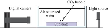
The experimental set-up is sketched in figure 2. A single
 $\text{CO}_{2}$
bubble was injected on top of a flat smooth substrate submerged in a small unpressurized observation tank (
 $10~\text{cm}\times 5~\text{cm}\times 5~\text{cm}$
) previously filled with distilled water at
 $20.5\,^{\circ }\text{C}$
. The distilled water was left openly exposed to ambient air for many hours beforehand to ensure air saturation. Two different substrate materials were employed: (a) PMMA (poly(methyl methacrylate)) and (b) collagen-coated coverslip glass.
Experimental set-up.

Before each experiment, the tank was emptied, and then rinsed and cleaned alongside the substrate with compressed air. The bubble injection was carried out manually by means of a needle connected to a pressurized
 $\text{CO}_{2}$
tank. The bubble was then left to dissolve for approximately six minutes. The whole dissolution process was optically recorded with a digital camera (TSI PowerView Plus 2MP Camera) acquiring at 2 f.p.s. The optical resolution was approximately
 $5~{\rm\mu}\text{m}~\text{pixel}^{-1}$
. The spherical cap radius
 $R$
and contact angle
 ${\it\theta}$
were then obtained through an image processing program developed in Matlab (see figure 4 below). The circular arc contour of the SCB was detected and a circle was fitted, from which the SCB radius
 $R$
could be immediately computed. The contact angle was then simply measured as
 ${\it\theta}=\arccos (h/R)$
, where
 $h$
is the circle centre height above the contact surface.
3.2. Experimental results
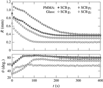
The experimental results for a selection of four SCBs are shown in figure 3, where their measured bubble radii and contact angles are plotted against time. The two bubbles adhered to the PMMA substrate shall henceforth be referred to as
 $\text{p}_{1}$
and
 $\text{p}_{2}$
. Likewise, those adhered to the glass coverslip shall be identified as
 $\text{g}_{1}$
and
 $\text{g}_{2}$
.
Experimental results for the evolution in time of the spherical cap radius
 $R$
and contact angle
 ${\it\theta}$
for four different SCBs. The two bubbles tested on the PMMA substrate (shaded markers) are termed
 $\text{p}_{1}$
and
 $\text{p}_{2}$
; the remaining two, tested on the glass substrate (white markers), are referred to as
 $\text{g}_{1}$
and
 $\text{g}_{2}$
.

Snapshots portraying the dissolution process of an SCB (corresponding to SCB
 $\text{g}_{2}$
) adhered to the coverslip glass substrate, taken at (a)
 $t=50~\text{s}$
, (b)
 $t=70~\text{s}$
, (c)
 $t=100~\text{s}$
and (d)
 $t=150~\text{s}$
. The SCB has been marked with the image-processed spherical cap contour (dotted curve) and the true height of the contact line (solid line).

The first particularity of interest is that the SCBs eventually attain a stable equilibrium size that signals the end of the dissolution process. This is a clear indicator of saturation of the liquid phase. It stands to reason since, as previously mentioned, the water was prepared to be air-saturated. This implies the diffusion-driven exchange of multiple gases across the SCB boundary. Initially, the SCB is composed purely of
 $\text{CO}_{2}$
, while the
 $\text{CO}_{2}$
concentration in the air-saturated water solution is effectively zero. The dissolution process is thus characterized by the simultaneous dominant outflow and modest inflow of
 $\text{CO}_{2}$
gas and air respectively. The equilibrium size is attained as soon as the bubble has been depleted of
 $\text{CO}_{2}$
, inferring that the bubble must be entirely composed of air thereafter.
It must be acknowledged, however, that in reality the air bubble is not strictly in equilibrium. The pressure inside the bubble will always be slightly higher than that of the surrounding liquid due to the Laplace pressure. This means that the bubble will, in fact, continue dissolving, but at a very slow rate. The dissolution time,
 $t_{d}$
, for an isolated single gas species spherical bubble immersed in a saturated gas–liquid solution may be quantified by appealing to a particular result from Epstein & Plesset (Reference Epstein and Plesset1950). In this case, the sole driving force is the liquid–gas surface tension. The bubble lifetime may approximated to be
 $$\begin{eqnarray}t_{d}\approx \frac{R_{0}^{3}p_{\infty }}{6D_{i}H\bar{R}T{\it\gamma}_{lg}},\end{eqnarray}$$
where
 $R_{0}$
denotes the initial bubble radius. As an example, air bubbles of initial radii
 $R_{0}=0.2$
and 0.5 mm have expected lifetimes of
 $t_{d}\sim 12~\text{h}$
and 8 days respectively. This confirms that this final stage of complete dissolution takes place on a much longer time scale than our time scale of interest, i.e. that encompassing the
 $\text{CO}_{2}$
–air exchange, which is shown to be of the order of a few minutes. At this latter time scale, it is therefore reasonable to neglect the effect of surface tension, and the bubbles may be thought to reach a final equilibrium size.
A second important feature is the advancing contact line pinning exhibited by every SCB. To better illustrate this phenomenon, a sequence of photographs depicting the dissolution of SCB
 $\text{g}_{2}$
are included in figure 4. It may be noted from snapshots (a) and (b) that the contact radius remains constant while the contact angle increases until in snapshot (c) the advancing contact angle,
 ${\it\theta}_{a}$
, is reached. Thereafter, in snapshot (d) the contact line decreases while the contact angle is practically fixed at
 ${\it\theta}_{a}$
. For PMMA, the advancing contact angles always exhibited consistent values between 80° and 85°. As one may note from figure 3, the coverslip glass surface apparently displayed weaker hydrophobicity. Advancing contact angles ranged from 55° to as much as
 $80^{\circ }$
.
The contact line behaviour that we observe in our experiments is analogous to the most common manner in which (macroscopic) sessile droplets evaporate. Stauber et al. (Reference Stauber, Wilson, Duffy and Sefiane2014) name this behaviour as the ‘stick–slide’ mode, in which the droplet first evaporates in a constant contact radius phase, followed by a sliding phase at a constant contact angle. The advancing contact angle is referred to as the transition contact angle instead. For microscopic SCBs, the contact line dynamics is likely to show great dependence on surface inhomogeneities and local defect pinning. A consequence of this is the intermittent contact line pinning (‘stick–jump’ mode) exhibited by evaporating surface nanodroplets (Dietrich et al. Reference Dietrich, Kooij, Zhang, Zandvliet and Lohse2015). In contrast, the macroscopic size of our bubbles averages the existing local defect pinning, thus rendering it unobservable.
4. Quasi-stationary dissolution model
4.1. Model equations
In this section we shall develop a mathematical model of the dissolution or growth of a multicomponent SCB adhered to a flat surface. This model is based on the quasi-stationary approximation, in which the concentration field may be uncoupled from the bubble boundary dynamics. The effect of advection is thence not considered. Furthermore, the concentration field of the surrounding liquid shall be approximated as radially symmetric, identical to that in the case of a fully spherical isolated bubble.
Consequently, the centre of the bubble may be taken as the origin of the radial coordinate
 $r$
, and we may proceed to solve the diffusion equation with spherical symmetry subject to a stationary boundary condition at
 $r=R$
. The concentration gradient at the bubble boundary has a well-known analytical solution that was first derived by Epstein & Plesset (Reference Epstein and Plesset1950). The equivalent expression applied to the
 $i$
th gas species in a multiple gas system (Weinberg & Subramanian Reference Weinberg and Subramanian1980) reads
 $$\begin{eqnarray}\left.\frac{\partial C_{i}}{\partial r}\right|_{r=R}=(C_{\infty ,i}-C_{s,i})\left[\frac{1}{R}+\frac{1}{\sqrt{D_{i}{\rm\pi}t}}\right].\end{eqnarray}$$
However, as briefly discussed in § 1, the flat plate has a slowing effect on the bubble dissolution and growth rates. The radial symmetry of the concentration field is broken in the region near the contact line, where the presence of weaker gradients implies a notable reduction in mass transport.
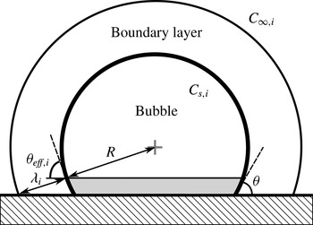
Sketch illustrating the effect of the plate on the effective bubble surface area. The excluded cap area (shaded region) is computed by determining the cone formed by the centre of the SCB and the intersection of the diffusion boundary layer (outer sphere) with the plate.

It is convenient to treat this effect as a mere reduction in the area available for mass transfer and assume that the concentration field remains spherically symmetric. The interaction of the boundary layer with the plate may be modelled following the approach proposed by Enríquez et al. (Reference Enríquez, Sun, Lohse, Prosperetti and van der Meer2014). The effective spherical cap area,
 $S_{eff,i}(t)$
, across which mass transfer of the
 $i$
th gas species is allowed, is dependent on the boundary layer thickness
 ${\it\lambda}_{i}(t)$
, and it is estimated as shown in figure 5. The effective area may be defined in an analogous manner to the true area by
 $S_{eff,i}={\rm\pi}{\it\beta}_{eff,i}R^{2}$
. From a simple geometrical calculation, one has that
 $$\begin{eqnarray}{\it\beta}_{eff,i}=2(1+\cos {\it\theta}_{eff,i})=2\left(1+\frac{R}{R+{\it\lambda}_{i}}\cos {\it\theta}\right).\end{eqnarray}$$
It should be noted that as
 ${\it\theta}\rightarrow {\rm\pi}/2$
,
 ${\it\beta}_{eff,i}\rightarrow {\it\beta}_{1}$
, where
 ${\it\beta}_{1}$
has been defined in (2.4). This is consistent with the fact that a semispherical bubble preserves the spherical symmetry of the concentration field. The boundary layer thickness
 ${\it\lambda}_{i}$
may be approximated to be the diffusion length scale defined by Lee, McKechnie & Devereux (Reference Lee, McKechnie and Devereux2011):
 $\partial _{r}C_{i}|_{r=R}=(C_{\infty ,i}-C_{s,i})/{\it\lambda}_{i}$
. From (4.1) it follows that
 $$\begin{eqnarray}{\it\lambda}_{i}=\left[\frac{1}{R}+\frac{1}{\sqrt{D_{i}{\rm\pi}t}}\right]^{-1}.\end{eqnarray}$$
The molar flow rate, previously defined in (2.8), now becomes
 $$\begin{eqnarray}{\dot{n}}_{i}={\rm\pi}{\it\beta}_{eff,i}R^{2}D_{i}\left.\frac{\partial C_{i}}{\partial r}\right|_{r=R}={\rm\pi}R^{2}{\it\beta}_{eff,i}D_{i}\left(C_{\infty ,i}-\frac{n_{i}}{n}p_{\infty }H_{i}\right)\left[\frac{1}{R}+\frac{1}{\sqrt{D_{i}{\rm\pi}t}}\right],\end{eqnarray}$$
and hereby the quasi-stationary model (QSM) is finally closed.
It is convenient to non-dimensionalize the system of the model equations. This may be done by introducing a dimensionless time
 ${\it\tau}$
, radius
 $a({\it\tau})$
,
 $i$
th species mole number
 ${\it\mu}_{i}({\it\tau})$
, total mole number
 ${\it\mu}({\it\tau})$
and finally the mole fraction of the
 $i$
th species
 $x_{i}({\it\tau})$
, as follows:
 $$\begin{eqnarray}{\it\tau}=\frac{D_{m}}{{R_{0}}^{2}}t,\quad a=\frac{R}{R_{0}},\quad {\it\mu}_{i}=\frac{\bar{R}T_{\infty }}{{\rm\pi}R_{0}^{3}p_{\infty }}n_{i},\quad {\it\mu}=\mathop{\sum }_{i=1}^{N}{\it\mu}_{i},\quad x_{i}=\frac{n_{i}}{n}=\frac{{\it\mu}_{i}}{{\it\mu}}.\end{eqnarray}$$
Here,
 $R_{0}$
is the characteristic bubble radius, which in this work is set to be the initial radius, i.e.
 $R_{0}=R(0)$
;
 $D_{m}$
stands for the mean value of the diffusivities. With strict regard to the formulation of the model final equations, it was deemed more propitious to dispose of the mole fraction,
 $x_{i}$
, in favour of
 ${\it\mu}_{i}$
and
 ${\it\mu}$
. Nonetheless, its usefulness will become evident later when specifying the initial bubble composition, and especially in § 5 where an approximate analytical solution shall be discussed. Let us now define the following dimensionless quantities:
 $$\begin{eqnarray}{\it\Upsilon}_{i}=\frac{\bar{R}T_{\infty }}{p_{\infty }}C_{\infty ,i},\quad {\it\Lambda}_{i}=\bar{R}T_{\infty }H_{i},\quad {\it\Gamma}_{i}=\frac{D_{i}}{D_{m}},\end{eqnarray}$$
where
 ${\it\Upsilon}_{i}$
refers to the initial concentration conditions in the liquid,
 ${\it\Lambda}_{i}$
serves as the solubility parameter and
 ${\it\Gamma}_{i}$
is a diffusivity ratio.
Hereupon, making use of the prime (
 $\text{}^{\prime }$
) to denote
 $\text{d}/\text{d}{\it\tau}$
, the QSM equations in dimensionless form are presented:
 $$\begin{eqnarray}\displaystyle & \displaystyle a^{\prime }=\frac{1}{{\it\beta}_{2}a^{2}}\mathop{\sum }_{i=1}^{N}{\it\mu}_{i}^{\prime }+\frac{{\it\beta}_{3}}{{\it\beta}_{2}}a{\it\theta}^{\prime }, & \displaystyle\end{eqnarray}$$
 $$\begin{eqnarray}\displaystyle & \displaystyle {\it\mu}_{i}^{\prime }={\it\beta}_{eff,i}a^{2}{\it\Gamma}_{i}\left({\it\Upsilon}_{i}-\frac{{\it\mu}_{i}}{{\it\mu}}{\it\Lambda}_{i}\right)\left[\frac{1}{a}+\frac{1}{\sqrt{{\it\Gamma}_{i}{\rm\pi}{\it\tau}}}\right],\quad i=1,\dots ,N, & \displaystyle\end{eqnarray}$$
 $$\begin{eqnarray}\displaystyle & \displaystyle {\it\theta}^{\prime }=\left\{\begin{array}{@{}ll@{}}-a^{\prime }\tan {\it\theta}/a,\quad & \text{if}~a^{\prime }<0\text{ and }{\it\theta}<{\it\theta}_{a},\\ 0,\quad & \text{otherwise},\end{array}\right. & \displaystyle\end{eqnarray}$$
 $$\begin{eqnarray}\displaystyle & \displaystyle \text{where }{\it\beta}_{eff,i}=2\left(1+\frac{a+\sqrt{{\rm\pi}{\it\Gamma}_{i}{\it\tau}}}{a+2\sqrt{{\rm\pi}{\it\Gamma}_{i}{\it\tau}}}\cos {\it\theta}\right),\quad i=1,\dots ,N. & \displaystyle\end{eqnarray}$$
The differential equations of this system may be solved numerically, subject to the initial conditions
 $a(0)=1$
,
 ${\it\theta}(0)={\it\theta}_{0}$
and
 ${\it\mu}_{i}(0)=x_{i}(0){\it\beta}_{2}({\it\theta}_{0})/3$
. In addition,
 ${\it\theta}_{a}$
must be known. It should be noted that the model is devoid of free parameters.
4.2. Experimental validation of model
The QSM was tested against the experimental results for
 $\text{CO}_{2}$
SCBs dissolving in air-saturated water. The experimental scenario is treated as a binary system (
 $N=2$
). Species
 $i=1$
refers to
 $\text{CO}_{2}$
gas, while air is conveniently approximated as a single species and may be correspondingly denoted by
 $i=2$
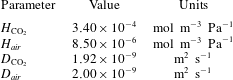
. The values of their diffusivities and Henry’s coefficients are given in table 1.
Values of the gas properties (at
 $p_{\infty }=10^{5}$
Pa and
 $T_{\infty }=293.5~\text{K}$
) used in this work. Values for
 $H_{i}$
and
 $D_{i}$
are taken from Cussler (Reference Cussler1997) and Sander (Reference Sander2014) respectively.

Previous works dealing with similar scenarios have treated air as an ideal binary mixture of
 $\text{N}_{2}$
and
 $\text{O}_{2}$
(Shim et al.
Reference Shim, Wan, Hilgenfeldt, Panchal and Stone2014). It must be mentioned that in this work, the dissolved air in water is in fact implicitly treated as a mixture composed of 64 %
 $\text{N}_{2}$
and 36 %
 $\text{O}_{2}$
by volume. This results simply from considering the solubilities in water of ambient air (taken as 79 %
 $\text{N}_{2}$
and 21 %
 $\text{O}_{2}$
). Since
 $\text{N}_{2}$
and
 $\text{O}_{2}$
have similar diffusivities (Cussler Reference Cussler1997), the evolutions of both concentration fields will be likewise similar. Their solubilities are also of the same order (Sander Reference Sander2014). Moreover, in this particular scenario, diffusion naturally establishes the equilibrium air composition of the bubble at the end of the dissolution process to be the same as the initial air composition dissolved in the (infinite) liquid medium, regardless of the difference in solubilities and diffusivities within the air mixture. For these reasons, it is acceptable to compute the mean solubility and diffusivity of the air mixture and treat air as a single gas species.
Finally, it is assumed that the SCB is initially composed purely of
 $\text{CO}_{2}$
, hence
 $x_{1}(0)=1$
,
 $x_{2}(0)=0$
. The air–water solution is initially saturated, i.e.
 ${\it\Upsilon}_{2}={\it\Lambda}_{2}$
, and
 $\text{CO}_{2}$
-deprived,
 ${\it\Upsilon}_{1}=0$
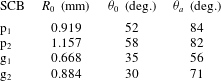
. The remaining input parameters, namely the initial geometry of the SCB and its advancing contact angle, are listed in table 2.
Experimentally determined values of the initial radius, initial contact angle and advancing contact angle corresponding to the four SCB dissolution experiments.

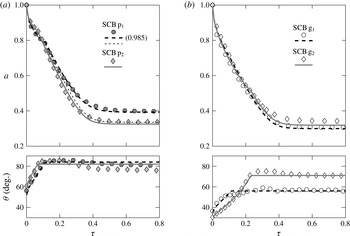
The comparison of the model with the experiments is shown in figure 6. The model solutions are in good agreement with the experimental data. It is verified that the contact angle dynamics is suitably described by the adhesion hysteresis model. One can notice that for bubbles
 $\text{p}_{1}$
and
 $\text{p}_{2}$
, the model solution for
 $a({\it\tau})$
succeeds in capturing the sudden change in slope at
 ${\it\tau}\approx 0.1$
. This is a consequence of the sharp transition from contact line pinning to contact line slip at the advancing angle.
Dimensionless radius
 $a$
and contact angle
 ${\it\theta}$
versus dimensionless time
 ${\it\tau}$
as computed from the quasi-stationary dissolution model (lines), compared with the experimental results (markers) for SCBs adhered to (a) the PMMA and (b) the coverslip glass substrate. For bubble
 $\text{p}_{1}$
the thick dashed curve corresponds to initial
 $\text{CO}_{2}$
and air mole fractions of 0.985 and 0.015 respectively. The rest of the model curves (including the thin dashed line for SCB
 $\text{p}_{1}$
) are calculated with the assumption that the initial bubble composition is 100 %
 $\text{CO}_{2}$
gas.

The case of SCB
 $\text{p}_{1}$
is of special interest. Upon the assumption that the SCB is initially 100 %
 $\text{CO}_{2}$
, the predicted equilibrium radius is underestimated by a significant 16 %. Allowing for a small initial mole fraction of air (1.5 %) to be present inside the bubble completely eliminates this difference. This in turn demonstrates the great sensitivity of the solution to the initial mole fraction. It is likely that SCB
 $\text{p}_{1}$
was not initially strictly 100 %
 $\text{CO}_{2}$
due to air entrapment within the valves and hoses connecting the
 $\text{CO}_{2}$
tank to the injection needle. Care was taken in purging the air out of the system before attempting the bubble injection process, yet for that experimental run we obviously failed to do so completely.
5. Approximate analytical solution
In this section we shall derive an approximate analytical solution of the radius dynamics meant to specifically model our dissolution scenario of interest, i.e. that of
 $\text{CO}_{2}~(i=1)$
bubbles dissolving in an air- (
 $i=2$
) saturated water solution. The solution itself has a twofold purpose: (a) to serve as a fast yet accurate means of calculating
 $R(t)$
and (b) to help in understanding the physical mechanisms that constitute this dissolution process. The baseline assumptions are identical to those stated for the generalized quasi-stationary dissolution model. Therefore, we shall adopt (4.7) to serve as our starting point.
Let us recall from § 4.2 that
 ${\it\Upsilon}_{1}=0$
and
 ${\it\Upsilon}_{2}={\it\Lambda}_{2}$
. Furthermore, we shall simplify the geometry of the bubble to that of a constant contact angle SCB (
 ${\it\theta}={\it\theta}_{a}$
) and ignore the effect of the plate on the diffusion boundary layer:
 ${\it\beta}_{eff,i}={\it\beta}_{1}({\it\theta}_{a})$
. It should be noted that setting
 ${\it\theta}_{a}=0$
will depict the case of an isolated fully spherical bubble. From here on, in an attempt to simplify the notation, we shall refer to the constants
 ${\it\beta}_{1}({\it\theta}_{a})$
and
 ${\it\beta}_{2}({\it\theta}_{a})$
simply as
 ${\it\beta}_{1}$
and
 ${\it\beta}_{2}$
respectively. Finally, it must be said that the following analysis is only valid when the solubility of gas 1 is much greater than that of gas 2, i.e.
 ${\it\Lambda}_{1}/{\it\Lambda}_{2}\gg 1$
(in our case,
 ${\it\Lambda}_{1}/{\it\Lambda}_{2}=40$
).
Upon inspection of (4.7b
), we find that the molar flow rate
 ${\it\mu}_{i}^{\prime }$
is proportional to the solubility parameter
 ${\it\Lambda}_{i}$
and the mole fraction
 $x_{i}={\it\mu}_{i}/{\it\mu}$
. A first stage of dissolution may be devised, during which the bubble radius is subject to a rapid decay. This regime is characterized by relatively large quantities of gas 1 diffusing out of the bubble since
 ${\it\Lambda}_{1}\gg {\it\Lambda}_{2}$
and
 ${\it\mu}_{1}\gg {\it\mu}_{2}$
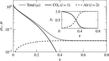
. The diffusive inflow of gas 2 is hence quite insignificant in comparison, and therefore may be assumed to have negligible impact on the bubble dynamics. This is observed in figure 7 – initially the curve for
 ${\it\mu}({\it\tau})$
is essentially identical to that for
 ${\it\mu}_{1}({\it\tau})$
. An analytical ‘short-time’ solution applicable to this regime shall be presented.
Dimensionless mole numbers
 ${\it\mu}_{i},{\it\mu}$
versus dimensionless time
 ${\it\tau}$
for SCB
 $\text{g}_{1}$
as computed from the QSM. Inset: equivalent mole fractions versus dimensionless time.

As time advances, however, the gas inflow must become increasingly important since it undoubtedly accounts for the eventual stabilization of the bubble radius. A long-time solution has also been developed for this second stage.
Rapid dissolution regime: short-time solution
The short-time solution is based on the approximation that
 $x_{1}\approx 1\gg x_{2}$
, and, in direct consequence,
 ${\it\mu}^{\prime }={\it\mu}_{1}^{\prime }$
. Following the workings detailed in appendix A, (4.7a
) becomes
 $$\begin{eqnarray}a^{\prime }=-\frac{{\it\Omega}}{2}\left(\frac{1}{\sqrt{1-{\it\Omega}{\it\tau}}}-\frac{1}{\sqrt{{\rm\pi}{\it\Gamma}_{1}{\it\tau}}}\right),\quad \text{where}~{\it\Omega}=2\frac{{\it\beta}_{1}}{{\it\beta}_{2}}{\it\Gamma}_{1}{\it\Lambda}_{1}.\end{eqnarray}$$
We may integrate (5.1) subject to the initial condition
 $a(0)=1$
, thereby obtaining the short-time solution:
 $$\begin{eqnarray}a=\sqrt{1-{\it\Omega}k{\it\tau}}-\frac{{\it\Omega}}{\sqrt{{\rm\pi}{\it\Gamma}_{1}}}\sqrt{k{\it\tau}},\quad \text{for}~{\it\tau}\in [0,{\it\tau}_{s}].\end{eqnarray}$$
We have introduced a free parameter
 $k$
(where
 $k\sim 0.5{-}1$
) that multiplies the time variable
 ${\it\tau}$
. It purposefully serves as a correction factor that may be determined through fitting, should it be deemed necessary to account for the effect of the plate on the concentration field; otherwise
 $k=1$
. The time
 ${\it\tau}_{s}$
, whose value is yet to be determined, marks an ‘idealized’ time limit after which the short-time solution ceases to be valid. For our particular dissolution scenario, by means of graphical estimation from figure 7, we may claim that
 ${\it\tau}_{s}\sim 0.2$
.
Radius stabilization regime: long-time solution
The long-time solution is likewise only valid for
 ${\it\tau}\geqslant {\it\tau}_{l}$
, where
 ${\it\tau}_{l}$
marks the beginning of the dissolution regime during which ideally the condition
 $\sqrt{{\rm\pi}{\it\Gamma}_{i}{\it\tau}}\gg a$
(or at least
 $\sqrt{{\rm\pi}{\it\Gamma}_{i}{\it\tau}}>a$
) is satisfied. The term
 $1/\sqrt{{\rm\pi}{\it\Gamma}_{i}{\it\tau}}$
in (4.7b
) may in such a case be neglected. The procedure for obtaining an integrable differential equation for the radius dynamics is given in appendix A. The result is
 $$\begin{eqnarray}a^{\prime }=\frac{{\it\beta}_{1}}{{\it\beta}_{2}}{\it\Gamma}_{2}{\it\Lambda}_{2}\left(\frac{1}{a^{4}}-\frac{1}{a_{eq}^{3}a}\right),\end{eqnarray}$$
where the final equilibrium radius,
 $a_{eq}$
, is also shown to be
 $$\begin{eqnarray}a_{eq}=\left(\frac{{\it\Gamma}_{2}{\it\Lambda}_{2}}{{\it\Gamma}_{1}{\it\Lambda}_{1}}\right)^{1/3}=\left(\frac{D_{2}H_{2}}{D_{1}H_{1}}\right)^{1/3}.\end{eqnarray}$$
To a good approximation, (5.4) reveals that the equilibrium radius just depends on the ratio of solubilities and diffusivities of both gases. It must be emphasized that this relation only applies to high-solubility gas (
 $\text{CO}_{2}$
) bubbles dissolving in a liquid saturated with a low-solubility gas (air).
We can now integrate (5.3) subject to the yet unknown transition condition
 $a({\it\tau}_{l})=a_{l}$
, where
 $a_{l}$
is the transition radius. The long-time solution reads
 $$\begin{eqnarray}\displaystyle k{\it\tau}-{\it\tau}_{l} & = & \displaystyle \frac{a_{eq}^{5}}{6}\frac{{\it\beta}_{2}/{\it\beta}_{1}}{{\it\Gamma}_{2}{\it\Lambda}_{2}}\left[\ln \left(\frac{(a_{eq}^{2}+a_{eq}a+a^{2})(a_{eq}-a_{l})^{2}}{(a_{eq}^{2}+a_{eq}a_{l}+a_{l}^{2})(a_{eq}-a)^{2}}\right)-2\sqrt{3}\arctan \left(\frac{2a+a_{eq}}{\sqrt{3}a_{eq}}\right)\right.\nonumber\\ \displaystyle & & \displaystyle \left.+\,2\sqrt{3}\arctan \left(\frac{2a_{l}+a_{eq}}{\sqrt{3}a_{eq}}\right)\right]+\frac{a_{eq}^{3}}{2}\frac{{\it\beta}_{2}/{\it\beta}_{1}}{{\it\Gamma}_{2}{\it\Lambda}_{2}}(a_{l}^{2}-a^{2}),\quad \text{for}~a\in [a_{l},a_{eq}].\nonumber\\ \displaystyle & & \displaystyle\end{eqnarray}$$
It should be noted that this solution asymptotically tends to the equilibrium radius,
 $a_{eq}$
. Nonetheless, the dissolution time may be graphically estimated.
Solution matching: transition criterion
In truth, there exists an intermediate transition time period (spanned by
 ${\it\tau}_{s}\lesssim {\it\tau}\lesssim {\it\tau}_{l}$
) where all terms in (4.7b
) are important. Judging from our results, the transition period may be regarded as relatively short. In such a case, the solution-matching problem is greatly simplified by imposing a sudden transition at time
 ${\it\tau}_{t}$
delimiting the applicability of the short-time from the long-time solution. Thus, we may approximate
 ${\it\tau}_{s}={\it\tau}_{l}={\it\tau}_{t}$
and
 $a_{s}=a_{l}=a_{t}$
.
The values of the transition time
 ${\it\tau}_{t}$
and corresponding radius
 $a_{t}$
are open to subjective determination, but should ultimately ensure the best possible agreement with any experimental or numerical data used as reference. For our particular dissolution scenario, experimental results showed that the long-time solution condition,
 $\sqrt{{\rm\pi}{\it\Gamma}_{i}{\it\tau}}\gg a$
, is in practice never attained – both terms remain at the same order of magnitude throughout the stabilization regime. Nonetheless,
 $\sqrt{{\rm\pi}{\it\Gamma}_{i}{\it\tau}_{t}}$
should at least be significantly larger than
 $a_{t}$
; a factor of 2 was regarded as a good compromise. The transition criterion here adopted is thus
 $$\begin{eqnarray}a_{t}=\frac{\sqrt{{\rm\pi}{\it\Gamma}_{1}{\it\tau}_{t}}}{2}.\end{eqnarray}$$
The analytical solutions to two distinct cases concerning the dissolution of a
 $\text{CO}_{2}$
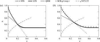
SCB in air-saturated water are plotted in figure 8. The equilibrium radius given by (5.4) proves to be remarkably accurate, provided that both gas diffusivities are similar, as is the case. In figure 8(b), the solutions are compared specifically with SCB
 $\text{g}_{1}$
since its contact angle displayed little variation (cf. figure 3) and thereby the constant contact angle approximation is valid. An empirically derived correction factor of
 $k=0.75$
was included to account for the presence of the flat plate.
Short-time analytical solution (STS) and long-time analytical solution (LTS) of the dissolution of a
 $\text{CO}_{2}$
SCB in air-saturated water. The transition point from the short-time to long-time solution is determined from the intersection of the transition criterion (dash-dot line) and the short-time solution. (a) Solutions for a semispherical bubble (
 ${\it\theta}_{a}=90^{\circ }$
,
 $k=1$
) compared with the solution from the QSM. The transition is at
 ${\it\tau}_{t}=0.21$
,
 $a_{t}=0.4$
. (b) Solution for an SCB with
 ${\it\theta}_{a}=56^{\circ }$
, compared with the experimental results for SCB
 $\text{g}_{1}$
. A correction factor of
 $k=0.75$
is used. The transition is at
 ${\it\tau}_{t}=0.29$
,
 $a_{t}=0.47$
.

Finally, it should be noted that the solutions have been extended beyond their valid timespan (thinner lines), outside which, as expected, the deviation becomes unacceptably large. This in turn endorses the validity of the transition criterion here proposed.
6. Finite-difference solution
It must be borne in mind that in § 4, the molar flow rates across the SCB interface were determined by assuming a quasi-stationary spherically symmetric concentration field together with a reduction in area accounting for the effect of the impermeable substrate. As a result of this approximation, Fick’s first law, (2.8), reduces to a simple expression corresponding to (4.7b ) in dimensionless form. The aim of this section is thus to provide a finite-difference method as an alternative means of determining the mass transfer of each gas species – ultimately serving as numerical validation for (4.7b ). More specifically, we seek to numerically solve for the concentration field from the diffusion equation confined to the real geometry of the system and subject to the authentic boundary conditions proposed in (2.2). This work shall then end with the subsequent comparison of the solutions obtained from both approaches.
6.1. Governing equations
For the sake of consistency with the previous developments, the finite-difference method equations shall be befittingly written in dimensionless form. We may begin by non-dimensionalizing both the molar concentration field,
 $C_{i}$
, and the interfacial concentration,
 $C_{s,i}$
, as follows:
 $$\begin{eqnarray}c_{i}=\frac{C_{i}-C_{\infty ,i}}{H_{i}p_{\infty }},\quad c_{s,i}=\frac{C_{s,i}-C_{\infty ,i}}{H_{i}p_{\infty }}.\end{eqnarray}$$
Rewriting (2.7) in dimensionless form yields a new expression for
 $c_{s,i}$
, which, when written in our notation, reads
 $$\begin{eqnarray}c_{s,i}=\frac{{\it\mu}_{i}}{{\it\mu}}-\frac{{\it\Upsilon}_{i}}{{\it\Lambda}_{i}}.\end{eqnarray}$$
Solving for the concentration in the physical
 $(x,y,z)$
domain is difficult since the SCB surface is a moving boundary. Instead, the dimensional Cartesian coordinates
 $(x,y,z)$
may be conveniently transformed to a dimensionless toroidal coordinate system
 $({\it\eta},{\it\xi},{\it\phi})$
, defined by
 $$\begin{eqnarray}\left.\begin{array}{@{}l@{}}\displaystyle x=R\sin {\it\theta}\frac{\sinh ({\it\theta}{\it\eta})}{\cosh ({\it\theta}{\it\eta})-\cos ({\it\theta}{\it\xi})}\cos {\it\phi},\\ \displaystyle y=R\sin {\it\theta}\frac{\sinh ({\it\theta}{\it\eta})}{\cosh ({\it\theta}{\it\eta})-\cos ({\it\theta}{\it\xi})}\sin {\it\phi},\\ \displaystyle z=R\sin {\it\theta}\frac{\sin ({\it\theta}{\it\xi})}{\cosh ({\it\theta}{\it\eta})-\cos ({\it\theta}{\it\xi})}.\end{array}\!\right\}\end{eqnarray}$$
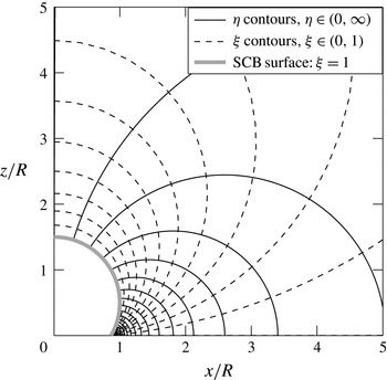
The contours of the coordinates
 ${\it\eta}$
and
 ${\it\xi}$
on the
 $x{-}z~(y=0,{\it\phi}=0)$
plane are shown in figure 9. In addition, the coordinate
 ${\it\phi}$
is defined as the angle of rotation about the
 $z$
-axis. This coordinate system is, of course, orthogonal. The scale factors are
 $$\begin{eqnarray}\left.\begin{array}{@{}c@{}}\displaystyle h_{{\it\eta}}=h_{{\it\xi}}=\frac{R{\it\theta}\sin {\it\theta}}{\cosh ({\it\theta}{\it\eta})-\cos ({\it\theta}{\it\xi})},\\ \displaystyle h_{{\it\phi}}=\frac{R\sin {\it\theta}\sinh ({\it\theta}{\it\eta})}{\cosh ({\it\theta}{\it\eta})-\cos ({\it\theta}{\it\xi})}.\end{array}\!\right\}\end{eqnarray}$$
Contours of the toroidal
 ${\it\eta}$
,
 ${\it\xi}$
coordinates plotted in the
 $y=0~({\it\phi}=0)$
Cartesian plane, with
 ${\it\theta}=60^{\circ }$
.

In these coordinates, the bubble surface lies on the
 ${\it\xi}=1$
isosurface regardless of the instantaneous radius
 $R(t)$
and contact angle
 ${\it\theta}(t)$
. The flat plate and infinity lie at
 ${\it\xi}=0$
. Lastly,
 ${\it\eta}\rightarrow \infty$
denotes the triple-contact line while
 ${\it\eta}=0$
maps onto the positive
 $z$
-axis (axis of symmetry). Furthermore, the rotational symmetry of the system in
 ${\it\phi}$
implies that
 $\partial /\partial {\it\phi}=0$
. Therefore, one must now only solve for a two-dimensional concentration field, namely
 $c_{i}=c_{i}({\it\eta},{\it\xi},{\it\tau})$
. The computational domain is therefore a fixed rectangular domain in (
 ${\it\eta},{\it\xi}$
) spanned by
 ${\it\eta}\in (0,\infty )$
and
 ${\it\xi}\in (0,1]$
.
The diffusion equation, namely (2.1), may be correspondingly transformed following the procedure detailed in appendix B. It is shown to be
 $$\begin{eqnarray}\frac{\partial c_{i}}{\partial {\it\tau}}=F\frac{\partial c_{i}}{\partial {\it\eta}}+G\frac{\partial c_{i}}{\partial {\it\xi}}+H\left(\frac{\partial ^{2}c_{i}}{\partial {\it\eta}^{2}}+\frac{\partial ^{2}c_{i}}{\partial {\it\xi}^{2}}\right),\end{eqnarray}$$
where
 $F$
,
 $G$
and
 $H$
are space- and time-dependent coefficients given by
 $$\begin{eqnarray}\displaystyle & \displaystyle F=\frac{1}{{\it\theta}}\left[\frac{{\it\Gamma}_{i}}{a^{2}\sin ^{2}{\it\theta}\sinh {\it\theta}{\it\eta}}(1-\cosh {\it\theta}{\it\eta}\cos {\it\theta}{\it\xi})(\cosh {\it\theta}{\it\eta}-\cos {\it\theta}{\it\xi})\right]-{\it\eta}^{\prime }, & \displaystyle\end{eqnarray}$$
 $$\begin{eqnarray}\displaystyle & \displaystyle G=\frac{1}{{\it\theta}}\left[-\frac{{\it\Gamma}_{i}}{a^{2}\sin ^{2}{\it\theta}}\sin {\it\theta}{\it\xi}(\cosh {\it\theta}{\it\eta}-\cos {\it\theta}{\it\xi})\right]-{\it\xi}^{\prime }, & \displaystyle\end{eqnarray}$$
 $$\begin{eqnarray}\displaystyle & \displaystyle H=\frac{{\it\Gamma}_{i}}{a^{2}{\it\theta}^{2}\sin ^{2}{\it\theta}}(\cosh {\it\theta}{\it\eta}-\cos {\it\theta}{\it\xi})^{2}. & \displaystyle\end{eqnarray}$$
Expressions for
 ${\it\eta}^{\prime }$
and
 ${\it\xi}^{\prime }$
are given in (B 2). The initial condition for the concentration is simply
 $c_{i}({\it\eta},{\it\xi}>1,0)=0$
, and the transformed boundary conditions are
 $$\begin{eqnarray}\left.\begin{array}{@{}ll@{}}\left.c_{i}\right|_{{\it\xi}=1}=c_{s,i},\quad & \text{imposition of the interfacial concentration},\\ \displaystyle \left.\frac{\partial c_{i}}{\partial {\it\xi}}\right|_{{\it\xi}=0}=0,\quad & \text{no flux across the wall},\\ \displaystyle \left.\frac{\partial c_{i}}{\partial {\it\eta}}\right|_{{\it\eta}=\infty }=0,\quad & \text{no flux across the bubble contact point},\\ \displaystyle \left.\frac{\partial c_{i}}{\partial {\it\eta}}\right|_{{\it\eta}=0}=0,\quad & \text{symmetry condition across the }z\text{-}\text{axis}.\end{array}\!\right\}\end{eqnarray}$$
The no-flux condition across the bubble contact line is imposed for mathematical convenience. The fact that the area of the contact line is infinitesimally thin means that mass transfer across it may be neglected. In other words, the final solution will thus essentially be impervious to the nature of that particular boundary condition. Moreover, it should be noted that these boundary conditions imply a suitable no-flux condition at infinity in the physical domain (corresponding to the intersection point of
 ${\it\eta}\rightarrow 0^{+}$
and
 ${\it\xi}\rightarrow 0^{+}$
isocontours).
Once the concentration field is known, the dimensionless molar flow rate
 ${\it\mu}_{i}^{\prime }$
may be computed through Fick’s first law, as shown in appendix B. This yields the following line integral:
 $$\begin{eqnarray}{\it\mu}_{i}^{\prime }=-2{\it\Gamma}_{i}{\it\Lambda}_{i}a\sin {\it\theta}\int _{0}^{\infty }\frac{\sinh {\it\theta}{\it\eta}}{\cosh {\it\theta}{\it\eta}-\cos {\it\theta}}\left.\frac{\partial c_{i}}{\partial {\it\xi}}\right|_{{\it\xi}=1}\,\text{d}{\it\eta}.\end{eqnarray}$$
The equations for the bubble radius and contact angle dynamics remain unchanged, as previously given by (4.7a ) and (4.7c ).
6.2. ‘Quasi-stationary’ and ‘fixed-particle’ finite-difference approximations
The coefficients
 $F$
and
 $G$
in (6.5b
) each contain a time-dependent velocity field, namely
 ${\it\eta}^{\prime }({\it\eta},{\it\xi},{\it\tau})$
and
 ${\it\xi}^{\prime }({\it\eta},{\it\xi},{\it\tau})$
respectively. In the upcoming work we shall set
 ${\it\eta}^{\prime }=0$
and
 ${\it\xi}^{\prime }=0$
on the grounds that the contribution of these terms is small – this constitutes the quasi-stationary approximation. This is equivalent to imposing a ‘scaling advection’ term,
 $\boldsymbol{U}_{\boldsymbol{S}}\boldsymbol{\cdot }\boldsymbol{{\rm\nabla}}C_{i}$
, in the diffusion equation (2.1) and solving it thereafter. Physically, this translates to fluid particles having the same velocity as that of our
 $R(t)$
and
 ${\it\theta}(t)$
scaling coordinate system. In fact, the velocity field turns out to be
 $\boldsymbol{U}_{\boldsymbol{S}}=-h_{{\it\eta}}\dot{{\it\eta}}\hspace{2.22198pt}\hat{\boldsymbol{e}}_{\boldsymbol{{\it\eta}}}-h_{{\it\xi}}\dot{{\it\xi}}\hspace{2.22198pt}\hat{\boldsymbol{e}}_{{\bf\xi}}$
. This field is non-physical: particles at the SCB interface will rightly have the interface velocity, but as we move away from the bubble, particles have increasing velocity as opposed to the decreasing velocity one would expect from continuity. This means that particles at infinity essentially move with infinite velocity. Fortunately, mass transfer is dictated by the gradients at the interface, where the scaling advection velocity,
 $U_{S}({\it\eta},1,{\it\tau})$
, equals the real advection velocity, i.e. the interface velocity. Moreover, the finite-difference quasi-stationary solution allows for a faithful comparison with the previous solutions presented in § 4 based on the same approximation.
On the other hand, keeping
 ${\it\eta}^{\prime }$
and
 ${\it\xi}^{\prime }$
in the expression is evidently consistent with rigorously solving (2.1), i.e. the diffusion equation strictly without advection. The consequence is that all fluid particles, even those at the interface, are deprived of any velocity in the physical domain. In other words, particles are forced to remain fixed in space always, whence the term ‘fixed-particle’ approximation. In summary, retaining these terms while neglecting the real advection is highly incongruent and defies mass conservation – a moving boundary forcefully implies the movement of neighbouring fluid particles – which ultimately may lead to significant physical errors.
These observations lead to the conclusion that the true solution, should the real velocity field be known, will lie within the quasi-stationary and fixed-particle solutions.
6.3. Comparison of solutions and experiment
Recalling the previous results presented in § 4.2, the finite-difference solution was likewise tested by modelling the same experimental scenarios. Equation (6.5) was solved numerically on a
 $200\times 100$
equispaced grid in the (
 ${\it\eta},{\it\xi}$
) plane, with
 ${\it\eta}\in [0.0001,10]$
and
 ${\it\xi}=[0.0001,1]$
. A first-order backward-time scheme and a second-order centred-space scheme were used.
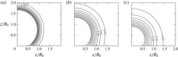
Figure 10 depicts the evolution of the
 $\text{CO}_{2}$
concentration field at the early stage of the dissolution process. It is computed using the input parameters corresponding to SCB
 $\text{g}_{2}$
. The diffusive symmetry of this binary problem implies that the dimensionless concentration field for air (
 $i=2$
) is identical to the one shown for
 $\text{CO}_{2}~(i=1)$
, except that the values of the contours are negative:
 $c_{2}=-0.02$
lies on
 $c_{1}=0.02$
, etc.;
 $c_{2}=0$
denoting saturation conditions. As may be noted from the evolution of the field contours from plot (b) to (c), the diffusive boundary layer is strongly advected towards the bubble, especially in the top region where the interface velocity is greatest. This is a consequence of the implicit scaling advection present in the quasi-stationary finite-difference approximation. Any contour sufficiently far away from the bubble is therefore expected to differ noticeably from the real solution.
Contours of
 $c_{1}$
, the dimensionless
 $\text{CO}_{2}$
concentration field, obtained when modelling SCB
 $\text{g}_{2}$
. Since
 $C_{\infty ,1}=0$
,
 $c_{1}$
is equivalent to the
 $\text{CO}_{2}$
saturation fraction in the water. Contours are plotted at dimensionless times (a)
 ${\it\tau}=0.01$
, (b)
 ${\it\tau}=0.06$
and (c)
 ${\it\tau}=0.15$
. The outermost contour shown is for
 $c_{1}=0.02$
, while the adjacent contour is for
 $c_{1}=0.1$
. The rest of the contours represent an increase in
 $c_{1}$
of 0.1; the SCB surface (thick grey line) is at
 $c_{1}=c_{s,1}({\it\tau})$
.

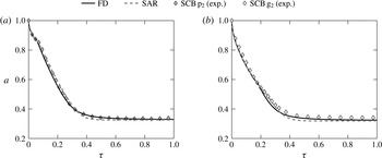
In figure 11, the finite-difference solution is compared with previous experimental results and solutions from the original model. Both methods appear to be in close agreement, thus numerically confirming the validity of determining mass transfer through (4.7b ). In addition, the quasi-stationary approximation, regardless of the method, proves to suitably predict the dynamics of dissolving bubbles subject to sufficiently mild driving forces. In such a case, the magnitude of the disparity between the implicit scaling advection and the real advection is small, and consequently has little effect on the bubble dynamics.
Dimensionless radius
 $a$
versus dimensionless time
 ${\it\tau}$
. The solutions computed by the finite-difference method (FD) are compared with experimental results for (a) SCB
 $\text{p}_{2}$
and (b) SCB
 $\text{g}_{2}$
. The previous solutions from figure 6 are also shown, where mass transfer is given by (4.7b
), i.e. considering a spherically symmetric concentration field alongside an area reduction treatment (SAR).

7. Conclusions
This work has addressed the fundamental problem of the diffusion-driven dissolution of a sessile SCB adhered to a flat homogenous surface. These bubbles are characterized by having contact angles much greater than zero. It is no surprise to find that the contact angle dynamics plays an important role in the bubble dissolution rate. In particular, we have performed experiments on the dissolution of
 $\text{CO}_{2}$
bubbles immersed in air-saturated water adhered to collagen-coated glass and PMMA substrates.
A quasi-stationary dissolution model for multicomponent SCBs has been devised, whose solutions have been compared with experimental data. The quasi-static contact angle behaviour is dictated by a simplified model based on the results obtained from adhesion hysteresis. Mass transfer of gas species across the bubble interfaces (Fick’s first law) has been computed through two methods.
-
(a) The concentration field is approximated as spherically symmetric. The effect of the impermeable substrate is treated as a reduction in the SCB area available for mass transfer based on a boundary layer–plate interaction model,
-
(b) A finite-difference method is developed in toroidal coordinates, where the concentration field is explicitly solved for, confined to the real geometry and subject to the real boundary conditions.
Both methods yield very close solutions – the evolution in time predicted for the SCB radius and contact angle compares very well with the experimental data. In addition, we have presented approximate analytical solutions that shed valuable insight on the nature of the diffusive processes that dictate the dissolution dynamics.
To conclude, a proper understanding and modelling of this fundamental problem may be regarded as the essential initial stage towards studying more realistic scenarios where bubbles are subject to higher degrees of confinement. An example would be bubble trapping in the pore spaces of underwater permeable strata.
Acknowledgements
The authors gratefully acknowledge the support of Total E&P Recherche et Développement through study agreement FR00006995, and the Spanish Ministry of Economy and Competitiveness through grant DPI2014-59292-C3-1-P. In addition, the authors would like to thank D. Moreno and D. Fuster for their helpful discussions.
Appendix A
A.1. Short-time solution procedure
The assumptions bluntly translate to setting
 ${\it\mu}_{1}={\it\mu}$
and
 ${\it\mu}_{2}^{\prime }=0$
. Equation (4.7a
) becomes
 $$\begin{eqnarray}a^{\prime }=-\frac{{\it\beta}_{1}}{{\it\beta}_{2}}{\it\Gamma}_{1}{\it\Lambda}_{1}\left(\frac{1}{a}+\frac{1}{\sqrt{{\rm\pi}{\it\Gamma}_{1}{\it\tau}}}\right).\end{eqnarray}$$
The exact solution to this differential equation may only be conveniently expressed in parametric form (Epstein & Plesset Reference Epstein and Plesset1950). Conversely, we shall derive an approximate solution of
 $a({\it\tau})$
via a simple iterative approach. The term
 $1/\sqrt{{\rm\pi}{\it\Gamma}_{1}{\it\tau}}$
is dominant at the very initial instants of time. The term
 $1/a$
dominates after some time has elapsed, in which case (A 1) approximates to
 $$\begin{eqnarray}a^{\prime }=-\frac{{\it\beta}_{1}}{{\it\beta}_{2}}\frac{{\it\Gamma}_{1}{\it\Lambda}_{1}}{a}.\end{eqnarray}$$
Integrating this equation subject to the initial condition
 $a(0)=1$
yields an expression for
 $a({\it\tau})$
:
 $$\begin{eqnarray}a=\left(1-2\frac{{\it\beta}_{1}}{{\it\beta}_{2}}{\it\Gamma}_{1}{\it\Lambda}_{1}{\it\tau}\right)^{1/2}=\sqrt{1-{\it\Omega}{\it\tau}}.\end{eqnarray}$$
Inserting this expression into (A 1) leads to an improved differential equation as given in (5.1).
A.2. Long-time solution procedure
Equation (4.7b
) may be rewritten in terms of the mole fraction
 $x_{2}$
as follows:
 $$\begin{eqnarray}{\it\mu}_{1}^{\prime }=-{\it\beta}_{1}a{\it\Gamma}_{1}{\it\Lambda}_{1}(1-x_{2}),\quad {\it\mu}_{2}^{\prime }={\it\beta}_{1}a{\it\Gamma}_{2}{\it\Lambda}_{2}(1-x_{2}).\end{eqnarray}$$
From the definition of
 ${\it\mu}_{i}$
, it follows that
 ${\it\mu}=V/{\rm\pi}R_{0}^{3}={\it\beta}_{2}a^{3}/3$
. Consequently we have
 $$\begin{eqnarray}{\it\mu}^{\prime }={\it\beta}_{2}a^{2}a^{\prime }=\frac{{\it\beta}_{1}}{{\it\beta}_{2}}a({\it\Gamma}_{2}{\it\Lambda}_{2}-{\it\Gamma}_{1}{\it\Lambda}_{1})(1-x_{2}).\end{eqnarray}$$
An ordinary differential equation for
 $x_{2}$
is readily available since
 $$\begin{eqnarray}x_{2}^{\prime }=\left(\frac{{\it\mu}_{2}^{\prime }}{{\it\mu}}-x_{2}\frac{{\it\mu}^{\prime }}{{\it\mu}}\right)=3\frac{{\it\beta}_{1}}{{\it\beta}_{2}}{\it\Gamma}_{2}{\it\Lambda}_{2}(1-x_{2})\left[1-\left(1-\frac{{\it\Gamma}_{1}{\it\Lambda}_{1}}{{\it\Gamma}_{2}{\it\Lambda}_{2}}\right)x_{2}\right].\end{eqnarray}$$
Using the chain rule
 $a^{\prime }=x_{2}^{\prime }\,\text{d}a/\text{d}x_{2}$
on (A 5) yields
 $$\begin{eqnarray}\frac{\text{d}a}{\text{d}x_{2}}=\frac{a}{3}\left(1-\frac{{\it\Gamma}_{1}{\it\Lambda}_{1}}{{\it\Gamma}_{2}{\it\Lambda}_{2}}\right)\left[1-\left(1-\frac{{\it\Gamma}_{1}{\it\Lambda}_{1}}{{\it\Gamma}_{2}{\it\Lambda}_{2}}\right)x_{2}\right]^{-1}.\end{eqnarray}$$
Integrating (A 7) subject to the initial condition
 $a(x_{2}=0)=1$
gives
 $$\begin{eqnarray}a=\left[1-\left(1-\frac{{\it\Gamma}_{1}{\it\Lambda}_{1}}{{\it\Gamma}_{2}{\it\Lambda}_{2}}\right)x_{2}\right]^{-1/3},\end{eqnarray}$$
wherefrom follows an expression for the final equilibrium radius:
 $$\begin{eqnarray}a_{eq}=a(x_{2}=1)=\left(\frac{{\it\Gamma}_{2}{\it\Lambda}_{2}}{{\it\Gamma}_{1}{\it\Lambda}_{1}}\right)^{1/3}=\left(\frac{D_{2}H_{2}}{D_{1}H_{1}}\right)^{1/3}.\end{eqnarray}$$
Appendix B
B.1. Non-dimensionalization of the diffusion equation
Recalling that
 $R=R_{0}a$
, the contours of
 ${\it\eta}$
and
 ${\it\xi}$
satisfy the following inverse relations (Arfken Reference Arfken1970):
 $$\begin{eqnarray}\displaystyle & \displaystyle \coth ({\it\theta}{\it\eta})=\frac{x^{2}+y^{2}+z^{2}+R_{0}^{2}a^{2}\sin ^{2}{\it\theta}}{2R_{0}\sqrt{x^{2}+y^{2}}a\sin {\it\theta}}, & \displaystyle\end{eqnarray}$$
 $$\begin{eqnarray}\displaystyle & \displaystyle \cot ({\it\theta}{\it\xi})=\frac{x^{2}+y^{2}+z^{2}-R_{0}^{2}a^{2}\sin ^{2}{\it\theta}}{2zR_{0}a\sin {\it\theta}}. & \displaystyle\end{eqnarray}$$
 ${\it\tau}$
yields
 $$\begin{eqnarray}\displaystyle & \displaystyle {\it\eta}^{\prime }=-\frac{{\it\theta}^{\prime }}{{\it\theta}}{\it\eta}+\frac{1}{{\it\theta}}\left(\frac{a^{\prime }}{a}+{\it\theta}^{\prime }\cot {\it\theta}\right)\sinh {\it\theta}{\it\eta}\cos {\it\theta}{\it\xi}, & \displaystyle\end{eqnarray}$$
 $$\begin{eqnarray}\displaystyle & \displaystyle {\it\xi}^{\prime }=-\frac{{\it\theta}^{\prime }}{{\it\theta}}{\it\xi}+\frac{1}{{\it\theta}}\left(\frac{a^{\prime }}{a}+{\it\theta}^{\prime }\cot {\it\theta}\right)\cosh {\it\theta}{\it\eta}\sin {\it\theta}{\it\xi}. & \displaystyle\end{eqnarray}$$
 ${\it\eta},{\it\xi}$
),
 $$\begin{eqnarray}\displaystyle \frac{\partial }{\partial t}C_{i}(x,y,z,t) & = & \displaystyle H_{i}p_{\infty }\frac{\text{d}{\it\tau}}{\text{d}t}\frac{D}{D{\it\tau}}c_{i}({\it\eta},{\it\xi},{\it\tau})\nonumber\\ \displaystyle & = & \displaystyle \frac{D_{m}H_{i}p_{\infty }}{R_{0}^{2}}\left(\frac{\partial c_{i}}{\partial {\it\tau}}+{\it\eta}^{\prime }\frac{\partial c_{i}}{\partial {\it\eta}}+{\it\xi}^{\prime }\frac{\partial c_{i}}{\partial {\it\xi}}\right).\end{eqnarray}$$
Making use of the scale factors defined in (6.4), the remaining term containing the Laplacian transforms to
 $$\begin{eqnarray}\displaystyle {\rm\nabla}^{2}C_{i}(x,y,z,t) & = & \displaystyle H_{i}p_{\infty }{\rm\nabla}^{2}c_{i}({\it\eta},{\it\xi},{\it\tau})\nonumber\\ \displaystyle & = & \displaystyle \frac{H_{i}p_{\infty }}{h_{{\it\eta}}h_{{\it\xi}}h_{{\it\phi}}}\left[\frac{\partial }{\partial {\it\eta}}\left(\frac{h_{{\it\xi}}h_{{\it\phi}}}{h_{{\it\eta}}}\frac{\partial c_{i}}{\partial {\it\eta}}\right)+\frac{\partial }{\partial {\it\xi}}\left(\frac{h_{{\it\phi}}h_{{\it\eta}}}{h_{{\it\xi}}}\frac{\partial c_{i}}{\partial {\it\xi}}\right)\right]\nonumber\\ \displaystyle & = & \displaystyle \frac{H_{i}p_{\infty }}{a^{2}R_{0}^{2}\sin ^{2}{\it\theta}}\left[\frac{1}{{\it\theta}^{2}}(\cosh {\it\theta}{\it\eta}-\cos {\it\theta}{\it\xi})^{2}\left(\frac{\partial ^{2}c_{i}}{\partial {\it\eta}^{2}}+\frac{\partial ^{2}c_{i}}{\partial {\it\xi}^{2}}\right)\right.\nonumber\\ \displaystyle & & \displaystyle +\,\frac{1}{{\it\theta}\sinh {\it\theta}{\it\eta}}(1-\cosh {\it\theta}{\it\eta}\cos {\it\theta}{\it\xi})(\cosh {\it\theta}{\it\eta}-\cos {\it\theta}{\it\xi})\frac{\partial c_{i}}{\partial {\it\eta}}\nonumber\\ \displaystyle & & \displaystyle \left.-\,\frac{1}{{\it\theta}}\sin {\it\theta}{\it\xi}(\cosh {\it\theta}{\it\eta}-\cos {\it\theta}{\it\xi})\frac{\partial c_{i}}{\partial {\it\xi}}\right].\end{eqnarray}$$
The dimensionless diffusion equation, (6.5), follows immediately.
B.2. Evaluation of the surface integral
The unit vector
 $\hat{\boldsymbol{n}}$
introduced in (2.8) points normally outwards from the SCB surface and is in fact equal to
 $-\hat{\boldsymbol{e}}_{{\bf\xi}}$
. Making use of the identities
 $$\begin{eqnarray}\displaystyle & \hat{\boldsymbol{n}}\,\text{d}S=-\hat{\boldsymbol{e}}_{{\bf\xi}}\,\text{d}S_{{\it\xi}}=-h_{{\it\eta}}h_{{\it\phi}}\,\text{d}{\it\eta}\,\text{d}{\it\phi}\hspace{2.22198pt}\hat{\boldsymbol{e}}_{{\bf\xi}}, & \displaystyle\end{eqnarray}$$
 $$\begin{eqnarray}\displaystyle & \displaystyle \boldsymbol{{\rm\nabla}}C_{i}=H_{i}p_{\infty }\left(\frac{1}{h_{{\it\eta}}}\frac{\partial c_{i}}{\partial {\it\eta}}\hat{\boldsymbol{e}}_{\boldsymbol{{\it\eta}}}+\frac{1}{h_{{\it\xi}}}\frac{\partial c_{i}}{\partial {\it\xi}}\hat{\boldsymbol{e}}_{{\bf\xi}}\right) & \displaystyle\end{eqnarray}$$
 $S$
lies on the
 ${\it\xi}=1$
isosurface, we can expand (2.8) as follows:
 $$\begin{eqnarray}\displaystyle {\dot{n}}_{i} & = & \displaystyle -D_{i}H_{i}p_{\infty }\int _{0}^{2{\rm\pi}}\int _{0}^{\infty }\left[\frac{h_{{\it\eta}}h_{{\it\phi}}}{h_{{\it\xi}}}\frac{\partial c_{i}}{\partial {\it\xi}}\right]_{{\it\xi}=1}\,\text{d}{\it\eta}\,\text{d}{\it\phi}\nonumber\\ \displaystyle & = & \displaystyle -2{\rm\pi}D_{i}H_{i}p_{\infty }R\sin {\it\theta}\int _{0}^{\infty }\frac{\sinh {\it\theta}{\it\eta}}{\cosh {\it\theta}{\it\eta}-\cos {\it\theta}}\left.\frac{\partial c_{i}}{\partial {\it\xi}}\right|_{{\it\xi}=1}\,\text{d}{\it\eta}.\end{eqnarray}$$
Non-dimensionalizing (B 7), namely through
 $$\begin{eqnarray}{\it\mu}_{i}^{\prime }=\frac{\bar{R}T_{\infty }}{{\rm\pi}R_{0}p_{\infty }D_{m}}{\dot{n}}_{i},\end{eqnarray}$$
finally results in (6.7).