
1. Introduction
Toroidal drops are encountered in various natural phenomena and industrial processes. They appear in rotating fluids (Fontelos, García-Garrido & Kindelán Reference Fontelos, García-Garrido and Kindelán2011; Pairam & Fernández-Nieves Reference Pairam and Fernández-Nieves2009), result following drop sedimentation in immiscible fluids (Kojima, Hinch & Acrivos Reference Kojima, Hinch and Acrivos1984; Baumann et al. Reference Baumann, Joseph, Mohr and Renardy1992; Machu et al. Reference Machu, Meile, Nitsche and Schaflinger2001; Sostarecz & Belmonte Reference Sostarecz and Belmonte2003; Bosse et al. Reference Bosse, Kleiser, Härtel and Meiburg2005), may exist as a consequence to an impact of a drop with solid surfaces (Renardy et al. Reference Renardy, Popinet, Duchemin, Renardy, Zaleski, Josserand, Drumright-Clarke, Richard, Clanet and Quéré2003), or follow deformation of drops subjected to outer flow (Zabarankin, Lavrenteva & Nir Reference Zabarankin, Lavrenteva and Nir2015; Zabarankin Reference Zabarankin2016; Ee et al. Reference Ee, Lavrenteva, Smagin and Nir2018; Banerjee et al. Reference Banerjee, Lavrenteva, Smagin and Nir2021) or other external fields (see e.g. Deshmukh & Thaokar Reference Deshmukh and Thaokar2013; Ghazian, Adamiak & Castle Reference Ghazian, Adamiak and Castle2013; Texier et al. Reference Texier, Piroird, Quéré and Clanet2013; Zabarankin Reference Zabarankin2017a,Reference Zabarankinb). A detailed discussion of these phenomena and of applications of the resulting toroidal drops can be found in, for example, Zabarankin et al. (Reference Zabarankin, Lavrenteva and Nir2015), Banerjee et al. (Reference Banerjee, Lavrenteva, Smagin and Nir2021) and Malik, Lavrenteva & Nir (Reference Malik, Lavrenteva and Nir2021).
Pairam & Fernández-Nieves (Reference Pairam and Fernández-Nieves2009) proposed a method for the controlled generation of toroidal drops inside an immiscible fluid: a liquid is extruded from an injection needle into a rotating continuous phase until the resultant jet closes into a torus. It was found that when both phases are Newtonian, the resulting torus is unstable and it either breaks up into several drops or it shrinks, coalesces onto itself and forms a single drop. Mehrabian & Feng (Reference Mehrabian and Feng2013) reported on the numerical simulation of the breakup of a liquid torus due to the development of three-dimensional capillary instability. Fragkopoulos et al. (Reference Fragkopoulos, Pairam, Berger, Segre and Fernández-Nieves2017) used a particle image velocimetry method to experimentally obtain the flow field inside shrinking toroidal droplets. Recently, Zheng et al. (Reference Zheng, Xie, Chen, Zhang, Liu and Chen2020) presented a systematic investigation of the dynamics of a toroidal drop in viscous oil by varying the interfacial tension and viscosity of the outer phase.
A number of experimental studies of the dynamic behaviour of toroidal drops submerged into fluids for the cases of various rheology of the dispersed and continuous phases are available in the literature. Pairam et al. (Reference Pairam, Vallamkondu, Koning, van Zuiden, Ellis, Bates, Vitelli and Fernandez-Nieves2013) used a yield-stress outer fluid to stabilize a nematic toroidal drop. Pairam, Le & Fernández-Nieves (Reference Pairam, Le and Fernández-Nieves2014) studied the stability of toroidal droplets inside a yield-stress material and showed that two types of instability typical for simple fluids present also in this case. However, the elasticity of the outer medium can prevent either or both of these instabilities. Ellis et al. (Reference Ellis, Pearce, Chang, Goldsztein, Giomi and Fernandez-Nieves2018) employed water-based toroidal droplets containing the active nematic and stabilized with an oil-based yield-stress fluid as the continuous phase to study the dynamics of topological defects. Fragkopoulos et al. (Reference Fragkopoulos, Pairam, Marinkovic and Fernández-Nieves2018) used toroidal droplets to study the breakup dynamics of a Newtonian liquid jet in the presence of rheologically nonlinear materials and demonstrated the crucial role of both viscoelastic and shear-thinning properties of the outside material in the dynamic process.
Studies of the deformation of rotating drops date back to Plateau's experiments (Plateau Reference Plateau1843), where various non-spherical shapes, including toroidal shapes, were observed. Poincaré (Reference Poincaré1885) computed the equilibrium shapes of a rotating drop and found axisymmetric and asymmetric families of forms. After the work of Poincaré, the curiosity of exploring new equilibrium solutions of rotating drops increased and attracted many researchers (Rayleigh Reference Rayleigh1914; Chandrasekhar Reference Chandrasekhar1965; Brown & Scriven Reference Brown and Scriven1980; Myshkis et al. Reference Myshkis, Babskii, Kopachevskii, Slobozhanin, Tyuptsov and Wadhwa1987; Lyttleton Reference Lyttleton2013). Brown & Scriven (Reference Brown and Scriven1980) obtained branches of the solutions in which the axisymmetric rotating drop breaks down and may evolve to two-fold, three-fold or, in general,  $n$-fold symmetry. Heine (Reference Heine2006) showed that the branches of solutions with
 $n$-fold symmetry also contain toroidal forms. Wang et al. (Reference Wang, Trinh, Croonquist and Elleman1986) and Wang et al. (Reference Wang, Anilkumar, Lee and Lin1994) reported on experimental studies of the behaviour of acoustically rotated free drops in microgravity environment. It was observed that rotating drops displayed both ‘axisymmetric’ and ‘two-lobed’ shapes in the presence and absence of applied torques. These observations confirm the theoretically predicted existence of the distinct shape families and the bifurcation point between them. A detailed classification of all rotationally symmetric figures of equilibrium corresponding to rotating liquid masses subject to surface tension is given in Elms et al. (Reference Elms, Hynd, Lopez and McCuan2017). Nurse, Coriell & McFadden (Reference Nurse, Coriell and McFadden2015) studied the stability of rotating drops and showed that toroidal drops with a large aspect ratio (major radius to minor radius) are subject to azimuthal instabilities with higher mode numbers.
In the studies reviewed in the previous paragraph, the drops undergo solid body rotation and no other non-trivial flow is involved. More complicated than solid body rotation flow structure occurs if the deformation of the drops is dynamic or when a stationary drop is subjected to other types of outer flow. Numerical simulations on toroidal drop dynamics in viscous fluid based on the boundary integral formulation are reported in Stone & Leal (Reference Stone and Leal1989), Zabarankin et al. (Reference Zabarankin, Lavrenteva and Nir2015), Ee et al. (Reference Ee, Lavrenteva, Smagin and Nir2018) and Malik et al. (Reference Malik, Lavrenteva and Nir2021). Zabarankin & Nir (Reference Zabarankin and Nir2011) and Zabarankin (Reference Zabarankin2012, Reference Zabarankin2016) developed an alternative approach to the simulation of axisymmetric drop deformation based on generalized analytic functions. Direct numerical dynamic simulations of a toroidal drop freely suspended in an ambient fluid undergoing axisymmetric biextensional flow revealed that, depending on the ratio of viscous forces and surface tension and on initial conditions, the drop expands indefinitely when the initial major radius is sufficiently large or otherwise collapses to a singly connected shape. In-between these dynamic evolution patterns, the toroidal drop attains an intermediate near-steady shape that is preserved for a relatively long time (Zabarankin et al. Reference Zabarankin, Lavrenteva and Nir2015; Ee et al. Reference Ee, Lavrenteva, Smagin and Nir2018). These intermediate shapes are unstable to axisymmetric disturbances and, with the passage of time, they will either expand or contract. Thus, the obtained shapes only approximate real stationary solutions. Moreover, the direct method failed to find such stationary toroidal shapes with small inner radius.
An alternative method to identify stationary shapes of deformed drops is to minimize some norm of the normal velocity at the interface of the drop with respect to its shape. This method can be advantageous when compared with the one based on the direct simulation of the actual dynamics in finding stationary unstable solutions. However, complicated dependence of the interfacial velocity on the drop shape, and the fact that the corresponding functionals are unlikely to be convex, render it difficult to implement. Nevertheless, in the case when the drop interface is assumed to belong to some family of shapes, depending on a finite (desirably small) number of parameters, this method can be effective in finding approximate solutions. In the application to toroidal drops, this approach was discussed in Zabarankin et al. (Reference Zabarankin, Lavrenteva and Nir2015). Lavrenteva et al. (Reference Lavrenteva, Ee, Smagin and Nir2021) considered a three-parameter family of axisymmetric bodies with cross-sections of generalized Cassini ovals and obtained branches of stationary shapes of singly connected and toroidal drops embedded in axisymmetric biextensional flow.
Most of experimental and theoretical studies on dynamics and deformation of toroidal drops assume a single type of external forcing (e.g. rotation, compressional flow, electric or magnetic field). However, the highly nonlinear nature of the problem under consideration suggested non-trivial combined effects that may result from simultaneous application of complementary forces. Such effects were demonstrated in the recent studies of Zabarankin (Reference Zabarankin2016) for spheroidal drops in compressional flow under an electric field and Holgate & Coppins (Reference Holgate and Coppins2018) for charged rotating drops. Malik et al. (Reference Malik, Lavrenteva and Nir2021) studied drop deformation in a linear flow field having rotational and axisymmetric extensional or biextensional components. One of the most interesting results of Malik et al. (Reference Malik, Lavrenteva and Nir2021) is the existence of a subdomain of the physical parameters exhibiting stable stationary toroidal shapes of a rotating drop when under an extensional flow regime (stable to axisymmetric disturbances). Recall that if both phases are Newtonian fluids and in the absence of one of the components of the outer flow, all toroidal stationary shapes are unstable to these disturbances. Typically, the stable to axisymmetric disturbances solutions constructed by Malik et al. (Reference Malik, Lavrenteva and Nir2021) correspond to highly extended tori that are likely to be unstable to asymmetric disturbances (see, e.g. Pairam & Fernández-Nieves Reference Pairam and Fernández-Nieves2009; Nurse et al. Reference Nurse, Coriell and McFadden2015).
In this study, we employ the classical control theory to stabilize the unstable toroidal shapes obtained by Malik et al. (Reference Malik, Lavrenteva and Nir2021), and construct new ones in regions of the domain of parameters where direct numerical solutions failed to yield results. Methods of control theory are extensively and successfully employed to stabilize various types of flow, for example, for controlling the onset of turbulence and turbulence suppression in channel and pipe flow. A comprehensive review on the modern state of this subject can be found in Jovanović (Reference Jovanović2021). Fikl & Bodony (Reference Fikl and Bodony2021) developed optimal control methods for stationary and time-dependent deformation of a drop in viscous flow.
In the present work, we propose using a simple proportional-integral (PI) controller to stabilize axisymmetrical rotating toroidal drops affected by various configurations of external flow. The controlled variable is the intensity of the extensional component of the outer flow. The goal is to explore a large range of stationary solutions of the problem, most of which are unstable and hence are challenging to compute using the alternative methods mentioned earlier. Since the goal is finding those stationary solutions, and not the dynamic characteristics of the drop deformations around those solutions, the simple PI controller designed using a simplified model of the systems was demonstrated to suffice for the task at hand.
The manuscript is structured as follows. In § 2, a model of uncontrolled deformation of a toroidal drop under a combined action of rotation and axisymmetric extensional or compressional flow is formulated. The method for simulating the dynamic drop deformations based on quasistationary approximation and boundary integral equations is then introduced. This method is further utilized to simulate the dynamics of those deformations in unactuated and controlled settings. Section 3 is devoted to simplified models of drop deformations that are based on approximations of the drop-surrounding flow interface by simple shapes. The representations of the drop shape are expressed by finite number of variables (desirably low) and the derivation of their dynamic equations are presented. In § 4, we address the controller design aimed at stabilizing the toroidal drop deformation in a wide range of flow conditions. The design is based on the simplified models discussed earlier. The controller is incorporated into a simulation environment of the drop dynamics while using the simplified and full nonlinear models. The resulting stationary solutions are described, analysed and discussed in § 5. Finally, conclusions and perspectives for further work are presented § 6.
2. Dynamic drop deformation in linear viscous flow
2.1. Formulation of the problem
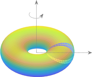
Consider a toroidal drop of volume  $V$, where
 $V$ equals the volume of sphere of radius
 $b$, density
 $\rho ^{(1)}$ and viscosity
 $\mu ^{(1)}$, embedded and deformed in an unbounded linear viscous flow. The outer fluid density and viscosity are
 $\rho ^{(2)}$ and
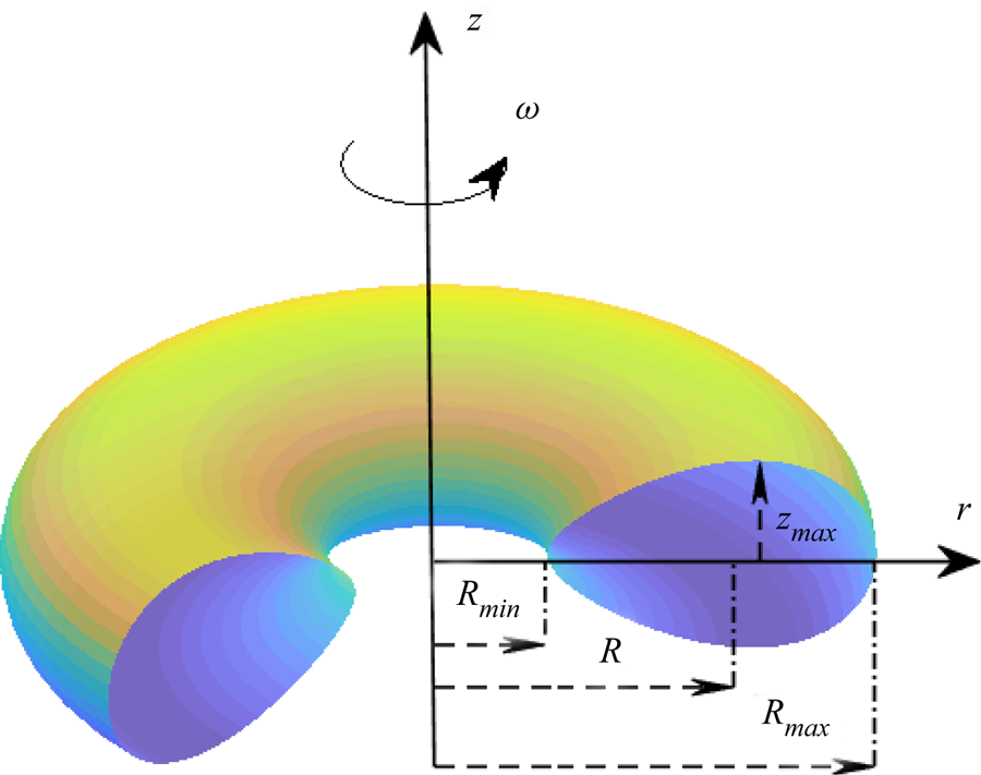
 $\mu ^{(2)}$, respectively (see figure 1). It is assumed that the fluids are immiscible.
A toroidal drop.

In the absence of the drop, the surrounding fluid is in linear velocity motion, that is a combination of rotation and extensional or biextensional (compressional) flow:
 \begin{equation} u_i^\infty = G_{ij} x_j+ \varepsilon_{ijk} \omega_j x_k. \end{equation}
Here,  $\boldsymbol {x} = x_i\boldsymbol {e}_i$ denotes the radius vector. The shear rate tensor
 $\boldsymbol{\mathsf{G}}$ is given by
 $G_{11}=G_{22}=G, G_{33}=-2G, G_{ij}=0$ when
 $i \neq j$, with
 $G$ being a constant characterizing the flow intensity, while
 $\omega _j=\omega \delta _{j3}$, with
 $\omega$ being the intensity of rotation. Positive and negative
 $G$ in (2.1) correspond to compressional and extensional modes of the flow, respectively.
Let  $\varOmega ^{(1)}$ denote the domain occupied by the drop,
 $\varOmega ^{(2)}$ the domain occupied by the ambient fluid, with
 $S$ being the interface between them. Let the velocity and pressure fields in
 $\varOmega ^{(i)}, i=1,2$, be denoted as
 $\boldsymbol {u}^{(i)}, p^{(i)}$, respectively. In what follows we assume creeping flow conditions neglecting inertia and gravitational sedimentation (Fontelos et al. Reference Fontelos, García-Garrido and Kindelán2011; Malik et al. Reference Malik, Lavrenteva and Nir2021). Under these assumptions and in a coordinate system rotating around the
 $x_3$-axis with a constant angular velocity
 $\omega$, these fields satisfy the equations
 \begin{equation} -\boldsymbol{\nabla} p^{(i)} +\mu^{(i)} \Delta \boldsymbol{u}^{(i)} -\rho^{(i)} \boldsymbol{\omega} \times ( \boldsymbol{\omega} \times \boldsymbol{x})=0, \quad \boldsymbol{\nabla} \boldsymbol{\cdot} \boldsymbol{u}^{(i)} =0, \quad \text{in} \ \varOmega^{(i)}, \ i=1,2. \end{equation}
At the interface, the continuity of the velocity is required, i.e.
 \begin{equation} \boldsymbol{u}^{(1)}=\boldsymbol{u}^{(2)}, \end{equation}
while at infinity  $\boldsymbol {u}^{(2)} \rightarrow \boldsymbol {u}^{\infty }$. The stress balance across the interface is of the form
 \begin{equation} \boldsymbol{\sigma}^{(2)}-\boldsymbol{\sigma}^{(1)}= \gamma H \boldsymbol{n}, \quad \text{on} \ S \end{equation}
with the interfacial tension  $\gamma$ being constant. Here,
 $\boldsymbol {\sigma }^{(i)}=- p^{(i)}+\mu ^{(i)}((\boldsymbol {\nabla } \boldsymbol {u}^{(i)}+ (\boldsymbol {\nabla } \boldsymbol {u}^{(i)})^{\rm T})/{2})$,
 $\boldsymbol {n}$ is a unit normal pointing outward into the ambient phase, and
 $H=\boldsymbol {\nabla } \boldsymbol {\cdot } \boldsymbol {n}$ is the surface mean curvature. The kinematic condition denoting the surface deformation is given by
 \begin{equation} U_n= u_n = \boldsymbol{u} \boldsymbol{\cdot} \boldsymbol{n}, \quad \text{on} \ S, \end{equation}
with  $U_n$ denoting the velocity of the interface in the normal direction. Introducing the modified pressure
 \begin{equation} P^{(i)}=p^{(i)}-\rho^{(i)} \frac{\omega^2 r^2}{2}, \quad \text{in} \ \varOmega^{(i)} \ i=1,2, \end{equation}
with  $r= |\boldsymbol {x}-(\boldsymbol {x} \boldsymbol {\cdot } \boldsymbol {e}_3)\boldsymbol {e}_3|= \sqrt {x_1^2+x_2^2}$ denoting the distance to the axis of rotation, reduces the above formulated problem to stationary Stokes equations with interfacial stress conditions of the form
 \begin{equation} \boldsymbol{\tau}^{(2)}-\boldsymbol{\tau}^{(1)}= \gamma H \boldsymbol{n}-(\rho^{(2)}- \rho^{(1)} ) \frac{\omega^2 r^2}{2}, \quad \text{on} \ S, \end{equation}
where  $\boldsymbol {\tau }^{(i)}=- P^{(i)}+\mu ^{(i)}(({\boldsymbol {\nabla } \boldsymbol {u}^{(i)}+(\boldsymbol {\nabla } \boldsymbol {u}^{(i)})^{\rm T}})/{2})$.
In what follows, throughout the paper, the length, and the velocity and the pressure fields are scaled with radius of the equivalent sphere  $b=({3V}/{4 {\rm \pi}})^{1/3}$, and
 $U^*=\gamma /\mu ^{(2)}$ and
 $\gamma /b$, respectively. The governing parameters of the problem are the viscosity ratio,
 $\lambda =\mu ^{(1)}/\mu ^{(2)}$, the capillary number,
 $Ca=\mu ^{(2)} b G/ \gamma$, and the rotational Bond number,
 \begin{equation} Bo=\frac{\left(\rho^{(1)}-\rho^{(2)}\right) \varOmega^2 b^3}{\gamma}. \end{equation}
Note that both capillary and Bond numbers can be negative. Positive and negative values of  $Ca$ correspond to compressional and extensional flow, respectively. Bond number is positive if the drop density exceeds that of the ambient fluid and negative otherwise.
For a given shape of the drop, the stationary Stokes equations (2.2), with boundary conditions (2.3) and (2.7), can be reduced to a system of integral equations for the velocity of the surface of the viscous drop,  $S$ given by (Rallison & Acrivos Reference Rallison and Acrivos1978; Pozrikidis Reference Pozrikidis1992)
 $$\begin{align} u_i(\boldsymbol{x}) &=
\left( \frac{2 Ca}{\lambda +1} \right) u_i^\infty
(\boldsymbol{x}) + \frac{2(1-\lambda)}{\lambda +1}
\oint_{S_y} K_{ijk}(\boldsymbol{x} - \boldsymbol{y}) u_j(\boldsymbol{y})
n_k(\boldsymbol{y}) \,{\rm d}S_y\nonumber\\ &\quad -
\frac{1}{\lambda +1}\oint_{S_y} J_{ij}(\boldsymbol{x} - \boldsymbol{y})
n_j(\boldsymbol{y}) \left(\frac{ \partial n_k}{\partial
x_k}(\boldsymbol{y})-\frac{Bo r_y^2}{2} \right) \,{\rm
d}S_y, \quad \boldsymbol{x} \in S,
\end{align}$$
where  $S_y$ is the surface of the drop. The kernels are given by
 \begin{equation} K_{ijk}(\boldsymbol{r})={-} \frac{3}{4 {\rm \pi}} \frac{r_i r_j r_k}{|\boldsymbol{r}|^5}, \quad J_{ij}(\boldsymbol{r})= \frac{1}{4 {\rm \pi}} \left(\frac{\delta_{ij}}{|\boldsymbol{r}|}+\frac{r_i r_j}{|\boldsymbol{r}|^3} \right). \end{equation}
In the particular case in which  $\lambda =1$, (2.9) reduces to the explicit expression
 \begin{equation} u_i(\boldsymbol{x}) = Ca \; u_i^\infty (\boldsymbol{x}) - \frac{1}{2}\oint_{S_y} J_{ij}(\boldsymbol{x} - \boldsymbol{y}) n_j(\boldsymbol{y}) \left(\frac{ \partial n_k}{\partial x_k}(\boldsymbol{y})-\frac{Bo r_y^2}{2} \right) \,{\rm d}S_y. \end{equation}
Given the axial symmetry of the drop under consideration, a cylindrical coordinate system  $(r, \phi, z)$ with basis
 $(\boldsymbol {e}_r, \boldsymbol {e}_\phi, \boldsymbol {e}_z)$ is used with the
 $z$-axis coinciding with the
 $x_3$-axis defined following (2.1). In this coordinate system, the undisturbed flow is given by
 $\boldsymbol {u}^\infty =r\boldsymbol {e}_r-2z\boldsymbol {e}_z$. Furthermore, the integral equations (2.9) are integrated over the angular coordinate,
 $\phi$, and are reduced to expressions containing curvilinear integrals over the cross-section of the drop interface
 $S$. The resulting expressions for the kernels can be found, for example in Pozrikidis (Reference Pozrikidis1992). For the particular case of
 $\lambda = 1$ addressed in this study, the velocity field is calculated directly from (2.11) while for other values of
 $\lambda$ the solution of (2.9) is established via an iterative procedure.
2.2. Dynamic deformations and stationary states
The algorithm for simulating dynamic deformations was to start the solution from some given shape and gradually advance it in a quasisteady manner in the normal direction making use of the kinematic condition. A detailed description of this approach can be found in Ee et al. (Reference Ee, Lavrenteva, Smagin and Nir2018) and Zabarankin et al. (Reference Zabarankin, Smagin, Lavrenteva and Nir2013, Reference Zabarankin, Lavrenteva and Nir2015). It was also used in Malik et al. (Reference Malik, Lavrenteva and Nir2021). In these studies, the simulations began from tori with a circular cross-section and a finite major radius,  $R$. It was demonstrated that when
 $R$ is small, the torus collapses to the axis, while for higher values of
 $R$, it expands indefinitely. When
 $R$ belongs to a certain interval, the shape stays visually unchanged for a relatively long time. The value of
 $R$ that yields the longest duration of stationary deformed toroidal shape with
 $\| U_n \| \ll 1$, both established to a desired degree of accuracy, is termed
 $R_{cr}$ and the resulting shape is accepted as a stationary solution.
These shapes vary from a torus of infinite extent (i.e.  $R_{max}\rightarrow \infty$) with a circular cross-section at
 $Ca \rightarrow 0$, via tori with finite radius having nearly oval cross-sections at intermediate
 $Ca$, to tori with shrinking inner radius at higher values of
 $Ca$ having cross-sections that resemble an egg shape. The solution of stationary almost collapsed shapes for each
 $\lambda$ could not be numerically established.
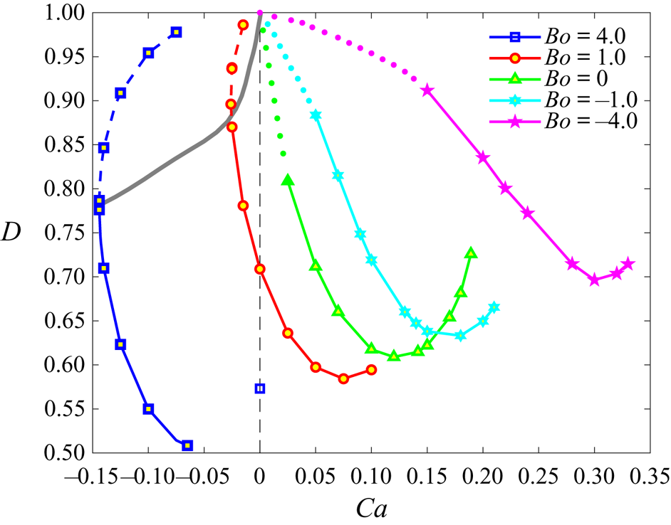
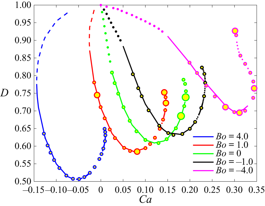
It was noted that in compressional flow, stationary toroidal shapes are unstable and, with the passage of time, they either collapse or expand due to unavoidable numerical disturbances. However, the combined action of rotation and extensional flow may result in toroidal shapes that are stable with respect to axisymmetric disturbances (see figure 2 reproduced from Malik et al. (Reference Malik, Lavrenteva and Nir2021)). The deformation factor,  $D$, for toroidal drop is defined as (Zabarankin et al. Reference Zabarankin, Lavrenteva and Nir2015)
 \begin{equation} D=\frac{R_{max}-z_{max}}{R_{max}+z_{max}}. \end{equation}
Phase plane of stable (dashed lines) and unstable (solid lines) stationary toroidal drops rotating in an axisymmetric linear flow. Here  $Ca>0$ and
 $Ca<0$ denote compressional and extensional flow, while
 $Bo>0$ and
 $Bo<0$, refer to heavy and light drops, respectively (Malik et al. Reference Malik, Lavrenteva and Nir2021).

An alternative method to find stationary solutions is to use an iterative procedure to minimize a norm of the normal velocity at the interface. For a stationary shape, this minimum should be zero. This method is not necessarily related to the actual dynamics of the drop and can be advantageous in finding unstable shapes. Especially, the effectiveness of such an approach is anticipated when the shape of the drop can be approximated by a simple geometric shape defined by a small number of parameters.
Several such approximations are available in the literature. Zabarankin et al. (Reference Zabarankin, Lavrenteva and Nir2015) approximate stationary drop shapes in the case of  $Bo = 0$ and
 $\lambda =1$ in the form of tori with circular and elliptic cross-sections. The parameters of the model are obtained by an inverse method: one of the parameters is fixed and the norm of the normal velocity is minimized with respect to
 $Ca$ and the remaining model parameters. This method is advantageous compared with the direct minimization due to a simple dependence of the functionals under consideration on
 $Ca$. The optimal
 $Ca$ is given by an explicit expression of the parameters of the model. For the one-parametric circular model, it gives the solution in the closed form, while for the two-parametric elliptic model, the problem is reduced to the minimization of a function of one parameter. The obtained ‘stationary’ elliptic solutions are shown to be in good agreement with the stationary shapes from quasidynamic simulations for almost the entire range of the capillary number, where the latter are available. The ‘stationary’ circular tori agree satisfactorily with the numerical shapes only for small values of
 $Ca$, however, they provide a quite good approximation for the starting point that leads to a stationary shape in numerical simulations. Lavrenteva et al. (Reference Lavrenteva, Ee, Smagin and Nir2021) suggested a generalized Cassini ovals approach for the approximation of both toroidal and simply connected stationary drops in compressional flow (
 $Bo=0$). Zabarankin et al. (Reference Zabarankin, Lavrenteva and Nir2015) also presented results of fitting the stationary shapes obtained by using quasidynamic simulations with shapes depending on a higher number of parameters.
Such approximation methods can be used for dynamic simulations as well. One can anticipate them to correctly describe the dynamics of the drop at least in the vicinity of stationary states. However, to the best of our knowledge, such approximate dynamic models were not used before. One family of such models is described in the following section. It will be used in the sequel for the control-based approach presented in this study.
3. Simplified dynamics for axisymmetric drops
3.1. General approach
Consider an  $N$-parametric family of bodies having the same volume as a unit sphere. Let the interface of a body,
 $S$, of this family be described by the parametric equations
 \begin{equation} \boldsymbol{x}= \boldsymbol{x}(\varphi, \theta, \boldsymbol{a}), \quad (\varphi, \theta) \in \varLambda, \quad \boldsymbol{a}=(a_1,\ldots, a_N), \end{equation}
with  $\varLambda$ denoting the domain of
 $(\varphi, \theta )$. Let the parameters of the body shape be functions of time,
 $a_i =a_i(t), \; i = 1,\ldots,N$. Then, the velocity of the interface in the normal direction is
 \begin{equation} U_n(\varphi, \theta, a_1,\ldots, a_N) = \frac{\partial \boldsymbol{x}}{\partial t} \boldsymbol{\cdot} \boldsymbol{n} =\left( \sum_{i=1}^N\frac{\partial\boldsymbol{x}}{\partial a_i} \frac{{\rm d} a_i}{{\rm d} t} \right) \boldsymbol{\cdot} \boldsymbol{n}= \sum_{i=1}^N\left(\frac{\partial\boldsymbol{x}}{\partial a_i} \boldsymbol{\cdot} \boldsymbol{n} \right) \frac{{\rm d} a_i}{{\rm d} t}. \end{equation}
Choose  $N$ points
 $\boldsymbol {\xi }_j = (\varphi _j, \theta _j) \in \varLambda$ and require that they comply with the kinematic conditions of (2.5) at all times
 $t$. This implies
 \begin{equation} \boldsymbol{A} \boldsymbol{\cdot} \frac{{\rm d} \boldsymbol{a}}{{\rm d} t} = \boldsymbol{B}, \end{equation}
where
 \begin{equation} A_{ij}=\frac{\partial\boldsymbol{x}_j}{\partial a_i} \boldsymbol{\cdot} \boldsymbol{n}(\boldsymbol{x}_j), \quad B_j = \boldsymbol{u}(\boldsymbol{x}_j) \boldsymbol{\cdot} \boldsymbol{n}(\boldsymbol{x}_j), \quad \text{at} \ \boldsymbol{x}_j= \boldsymbol{x}(\varphi_j, \theta_j, \boldsymbol{a}) \end{equation}
for all  $i=1,\ldots,N$,
 $j=1,\ldots, N$, and
 $\boldsymbol {u}(\boldsymbol {x}_j)$ is a solution of (2.9) for a given interface
 $S$ at point
 $(\boldsymbol {x}_j)$. It follows from (3.3) that
 \begin{equation} \frac{{\rm d} \boldsymbol{a}}{{\rm d} t} = \boldsymbol{A}^{{-}1} \boldsymbol{\cdot} \boldsymbol{B}, \end{equation}
which is the dynamics of the variables  $a_i$. Note that the choice of
 $\boldsymbol {\xi }_j$ should ensure the invertibility of
 $\boldsymbol {A}$. Note that
 $\boldsymbol {u}(\boldsymbol {x}_j)$ that defines the right-hand side of (3.3) depends on parameters
 $Ca$ and
 $Bo$, which can be used as control signal.
Stationary points,  $\mathbf {a}^0$, of (3.5) satisfy the highly nonlinear system of equations
 \begin{equation} \boldsymbol{B}( \boldsymbol{a}^0) = \boldsymbol{0}. \end{equation}
In the particular case of an axisymmetric toroidal drop that is symmetric also with respect to the  $z=0$ plane, it is convenient to consider only the upper part
 $z \geq 0$ of the drop shape and present the interface in the form
 \begin{gather} x = (a_1 + a_2 \cos \theta) \cos \varphi, \end{gather}
 \begin{gather}y = (a_1+a_2 \cos \theta) \sin \varphi, \end{gather}
 \begin{gather}z = \sin \theta \sum_{k=3}^N a_k \cos((k-3) \theta) = \sin \theta \sum_{k=3}^N a_k T_{(k-3)} (\cos \theta), \end{gather}
where  $N\geq 3$,
 $\varphi \in [0,2 {\rm \pi}), \theta \in [0,{\rm \pi} ]$,
 $T_k$ are the Chebyshev polynomials of the first kind, and the coefficients
 $a_k$ satisfy
 \begin{equation} {\rm \pi}a_2 (4 a_1 a_3 + a_2 a_4 - 2 a_1 a_5- a_2 a_6)= 8/3 \end{equation}
to ensure that the volume of the drop equals that of the unit sphere. If  $N<6$, (3.8) should be satisfied with
 $a_n=0$ for
 $n>N$. Note that for the stationary case, the representation in (3.7) and (3.8) coincides with the approximation used in Zabarankin et al. (Reference Zabarankin, Lavrenteva and Nir2015) that provided an excellent fitting of the numerically obtained stationary shapes with
 $N=7$.
3.2. Two-state model
The most simple case of surface given by (3.7) arises at  $N=3$. Due to the relation (3.8) this family of surfaces depend on two free parameters, that will serve as states in the dynamic equations. The drop interface in cylindrical coordinate system
 $(r,z)$ is described by
 \begin{equation} r=(a_1+a_2 \cos \theta),\quad z= \frac{2\sin \theta }{3 {\rm \pi}a_1 a_2 }. \end{equation}
Thus the drop is assumed to be an elliptic torus having a major radius  $a_1$ and a cross-section being an ellipse with axes
 $a_2$ and
 $2/(3 {\rm \pi}a_1 a_2)$. In what follows, we use the notations
 $a_1=R$ and
 $a_2=a=R-R_{min}$ (see figure 1). To construct the dynamic equations for those two parameters, we use the kinematic conditions at
 $\theta = 0$ and
 ${\rm \pi}$, i.e. at the points on the interface with coordinates
 $(R+a,0)$ and
 $(R-a,0)$. Due to the fore-and-aft symmetry of the interface,
 $u_z=0$ and
 $n_z=0$ at these points. After some simple manipulations, the dynamic system takes the form
 \begin{gather} \frac{{\rm d} R}{{\rm d} t} = f_1(R, a, Ca, Bo) =\frac{u_r(R+a,0,Ca,Bo)+u_r(R-a,0,Ca,Bo)}{2}, \end{gather}
 \begin{gather}\frac{{\rm d} a}{{\rm d} t} = f_2(R, a, Ca, Bo) =\frac{u_r(R+a,0,Ca,Bo)-u_r(R-a,0,Ca,Bo)}{2}, \end{gather}
where  $u_r$ are computed from (2.9). Note that the right-hand side of (3.10) are nonlinear functions of the model variables
 $R$ and
 $a$, and depend also on the flow characteristics defined by
 $Bo$ and
 $Ca$ numbers. The latter will be utilized when drop shape stabilization is addressed in the sequel.
The elliptic torus model, which was used in Zabarankin et al. (Reference Zabarankin, Lavrenteva and Nir2015) and Zabarankin (Reference Zabarankin2019) for identifying stationary solutions of toroidal drops, demonstrated a good agreement with the obtained relevant numerical solutions using the full model of (2.9) for small and intermediate capillary numbers. Recall, however, that in those studies the elliptical model was termed ‘stationary’ if an integral norm of the normal velocity component on the entire surface was minimal. If, in contrast to this procedure, the requirement is of zero normal velocity only at two points on the drop surface, it is necessary to verify if this condition provides satisfactory approximation for the stationary states of the full problem obtained by the numerical procedure when solving (2.9) or (2.11).
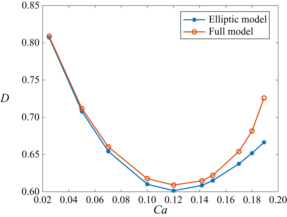
A comparison of the deformation of the stationary drop obtained by the elliptic torus model with that obtained by Malik et al. (Reference Malik, Lavrenteva and Nir2021) for non-rotating drops is shown in figure 3. Clearly, as the capillary number increases, the solution obtained using the elliptical model deviates from the results obtained by the full model. A similar trend is observed for rotating drops. It is noted that this deviation increases as the toroidal drop approaches the collapsed state where the actual shape of the cross-section becomes significantly different from an ellipse or even an oval. This is the region where accurate direct numerical solutions to the shapes are most difficult to compute.
Comparison of stationary drop deformation in compressional flow using the two-state model and full models (Malik et al. Reference Malik, Lavrenteva and Nir2021) for  $Bo=0$.

Nevertheless, the stationary solutions obtained via the elliptic model can be used as an initial approximation to be improved by applying a procedure that utilizes the full numerical model to better estimate the stationary deformation. Such a procedure, that involves feedback control, is discussed next.
4. Feedback control to determine stationary solutions
Rotating toroidal drops in Newtonian fluid are inherently unstable, except possibly for highly extended drops under extensional flow conditions (Malik et al. Reference Malik, Lavrenteva and Nir2021). Finding stationary solutions of the drop deformation in those unstable regions is numerically challenging. In this study, we propose a feedback-control-based scheme for finding those stationary solutions in a wide range of external flow conditions.
The procedure starts by stabilizing the unstable toroidal drop shape around a known solution and, relying on the robustness of the controller to model uncertainty and variations, find neighbouring stationary solutions. A linear feedback controller is designed using an approximate model of the drop deformation presented in the previous section. Consequently, the controller is robust only to limited variations in the model, i.e. in the flow conditions, when tested using the detailed nonlinear dynamic model of the system. Therefore, once the limit of flow variations is reached (beyond which a stationary solution cannot be found), a new controller is designed for the new stationary solution that is close to that limit. The process is repeated, covering the entire range of flow conditions of interest.
Note that the dynamic model, even the simplified one, is nonlinear. However, since our main goal is to find stationary solutions, and not perform advanced nonlinear regulation and tracking control tasks, we shall employ a linearization-based classical linear control design, using the simple model and a single-input–single-output controller.
In the present study, for any fixed  $Bo$, the control signal is chosen to be
 $Ca$. In a previous work (Malik et al. Reference Malik, Lavrenteva and Nir2021) it was found that for a fixed
 $Bo$,
 $R_{min}$ dictates a unique drop shape. Moreover, we are interested in finding the drop shapes collapsing towards the axis of symmetry. Therefore, the dictated control input and also the feedback signal that will be used by the controller is chosen as
 \begin{equation} R_{min}=R-a. \end{equation}
The control is designed on the basis of the approximate two-state model described in § 3.2. The states of this model are  $\boldsymbol {x}(t)=(R(t),a(t))$, and their nonlinear dynamics are governed by (3.10). For the controller design, this model is linearized, for a fixed
 $Bo$, around a known stationary solution
 $\boldsymbol {x_0}$, corresponding to
 $Ca=Ca_0$. The linearized model is given by
 \begin{gather} \delta \boldsymbol{\dot x}=\boldsymbol{A} \delta \boldsymbol{x}+ \boldsymbol{B} \delta Ca, \end{gather}
 \begin{gather}\delta R_{min}= \boldsymbol{C} \delta \boldsymbol{x} + \boldsymbol{D} \delta Ca, \end{gather}
where  $\boldsymbol {\dot x}$ denotes
 ${{\rm d} x}/{{\rm d}t}$ and
 \begin{align} \left. \begin{gathered} \boldsymbol{A}=\left[\frac{\partial \boldsymbol{f}}{\partial \boldsymbol{x}} \right]_{\boldsymbol{x_0}, Ca_0}=\left[ \begin{array}{cc} \dfrac{\partial f_1}{\partial R} & \dfrac{\partial f_1}{\partial a} \\ \dfrac{\partial f_2}{\partial R} & \dfrac{\partial f_2}{\partial a} \end{array} \right], \quad \boldsymbol{B}=\left[\frac{\partial \boldsymbol{f}}{\partial Ca} \right]_{\boldsymbol{x_0}}=\left[ \begin{array}{c} \dfrac{\partial f_1}{\partial Ca} \\ \dfrac{\partial f_2}{\partial Ca} \end{array} \right]=\left[ \begin{array}{c} R_0 \\ a_0 \end{array} \right],\\ \boldsymbol{C}=\left[\frac{\partial R_{min}}{\partial \boldsymbol{x}} \right]_{\boldsymbol{x_0}}=\left[ \begin{array}{cc} \dfrac{\partial R_{min}}{\partial R} & \dfrac{\partial R_{min}}{\partial a} \end{array} \right]=\left[ \begin{array}{cc} 1 & -1 \end{array} \right], \quad \boldsymbol{D}=\begin{array}{c} \left[\dfrac{\partial R_{min}}{\partial Ca} \right]_{\boldsymbol{x_0}}=0 \end{array}. \end{gathered} \right\} \end{align}
The partial derivatives in  $\boldsymbol {A}$ are calculated numerically by using a second-order central difference scheme. The open-loop transfer function between the control input
 $\delta Ca$ and the output
 $\delta R_{min}$, that will be used in the controller design, is given by
 \begin{equation} G_{ol} = \boldsymbol{C}\left(s\boldsymbol{I}-\boldsymbol{A}\right)^{{-}1}\boldsymbol{B}+\boldsymbol{D}, \end{equation}
where  $s$ is the complex Laplace variable and
 $\boldsymbol {I}$ is a
 $2\times 2$ identity matrix.
The uncontrolled process corresponds to  $Ca=Ca_0$, i.e.
 $\delta Ca=0$. If at least one eigenvalue of
 $\boldsymbol {A}$ in (4.2), or, equivalently, one of the poles of
 $G_{ol}(s)$, has a positive real part, then the stationary solution of (3.10) is unstable, i.e. due to small perturbations the toroidal drop with elliptic cross-section will either collapse or expand to infinity. As an example, consider the case of
 $Bo=-4, Ca_0=0.3$, for which an unstable stationary solution of the full problem (2.11) was found in Malik et al. (Reference Malik, Lavrenteva and Nir2021). A stationary solution of the two-state system (3.10) is
 $(R_0, a_0)=(1.1932, 0.5859)$, hence
 $R_{min,0}=0.6073$. The open-loop transfer function of (4.4) that corresponds to this
 $R_{min}$ is
 \begin{equation} G_{ol}(s)=\frac{0.2633(s+2.817)}{(s-0.229)(s+0.5033)}. \end{equation}
Evidently, one pole of system is negative and the other is positive. Thus, the two-state model at this  $Ca_0$ is unstable and the same is true for the full system, as was shown in Malik et al. (Reference Malik, Lavrenteva and Nir2021). Moreover, the system has a zero in the left-hand side of the complex
 $s$ plane, which is advantageous for stabilizing the unstable pole in (4.5) (Ogata Reference Ogata2010). The latter justifies the choice of the controlled output variable
 $R_{min}$ in (4.1).
In order to design a controller that stabilizes the system of (4.2) and also can generate a neighbouring solution defined by  $\delta R_{min}^D= R_{min}^D- R_{min,0}$, we introduce the error term between the desired and the calculated output
 \begin{equation} {e}(t)= R_{min}^D - R_{min}= \delta R_{min}^D- \delta R_{min}. \end{equation}
Since the transfer function in (4.5), and more generally in (4.4), does not have a pole at the origin, to ensure type one characteristics of the closed loop system, a PI controller will be used to stabilize the system (Ogata Reference Ogata2010). It is given by
 \begin{equation} \delta Ca={-}{K}_p \boldsymbol{e}-{K}_I \boldsymbol{e}_I, \end{equation}
where
 \begin{equation} \boldsymbol{\dot e}_I = \boldsymbol{e}. \end{equation}
Here  ${K}_p$ and
 ${K}_I$ are proportional and integral gains designed to stabilize the closed loop system. The integral component of the controller is introduced for robustness and to better account for the modelling errors caused by the simplified model. Also, this component will allow us to move from one stationary solution to the neighbouring one.
In the present study, the parameters  ${K}_p$ and
 ${K}_I$ are designed using the classical root locus tuning techniques. The transfer function of the controller for the sample case of the aforementioned example, i.e.
 $Bo=-4$ and
 $Ca=0.3$, is
 \begin{equation} C(s)=\frac{\delta Ca}{\boldsymbol{e}}(s)=K_p+\frac{K_I}{s}=\frac{5.565(s+0.279)}{s}. \end{equation}
The corresponding closed loop transfer function of the system is
 \begin{equation} G_{cl}(s)=\frac{\delta R_{min}}{\delta R_{min}^D}(s) = \frac{G_{ol}(s)C(s)}{1+G_{ol}(s)C(s)}= \frac{1.4653(s+2.817)(s+0.279)}{(s+0.2876)(s^2+1.452s+4.0037)}, \end{equation}
showing that the open loop system poles at  $(0.229,-0.5033)$ and the controller pole at the origin have been shifted by the controller to the stable left half-plane region and are located at
 $-0.726 \pm 1.8646i$ and
 $-0.2876$.
As discussed earlier, the above controller is used in the vicinity of the stationary solution  $\boldsymbol {x_0}$ to find neighbouring stationary shapes. This is carried out by applying this control logic to the full nonlinear model of the system (2.9). Since the linear controller computes only deviations in the capillary number, the value used in the simulations is given by
 $Ca=Ca_0+\delta Ca$, as is discussed next.
5. Control implementation to the full boundary integral equations
To design a controller that stabilizes the unstable solutions found in Malik et al. (Reference Malik, Lavrenteva and Nir2021), we chose a pair  $(Ca_0, Bo)$ for which this solution exists and find a stationary solution of the two-state model given by (3.10). We linearize this model in the vicinity of the stationary solution and design a controller, i.e. find the gains
 $K_p$ and
 $K_I$, as described above. Once the controller for the simplified model is established, it is applied to the full nonlinear dynamics model of (2.9) or (2.11) to determine neighbouring drop-shapes around the stationary solution above, dictated by
 $R_{min}=R_{min}^D$. Namely, in (2.11), the constant
 $Ca_0$ is dynamically changed as
 \begin{equation} Ca(t)= Ca_0 -{K}_p \left(R_{min}(t)- R_{min}^D\right)-{K}_I \int_0^t\left(R_{min}(\tau)- R_{min}^D\right)\,{\rm d}\tau, \end{equation}
where
 \begin{equation} R_{min}(t)=\min_{(r,z) \in S_t}(r). \end{equation}
For the initial conditions, we chose the established shape  $S_0$ corresponding to particular
 $(Ca_0, Bo)$, and some
 $R_{min}^D$ that is relatively close to
 $R_{min,0} =\min _{(r,z) \in S_0}(r)$. If the
 $R_{min}^D$ deviation is in fact small, due to the robustness of the controller, the simulation will converge to a neighbouring solution of the nonlinear model.
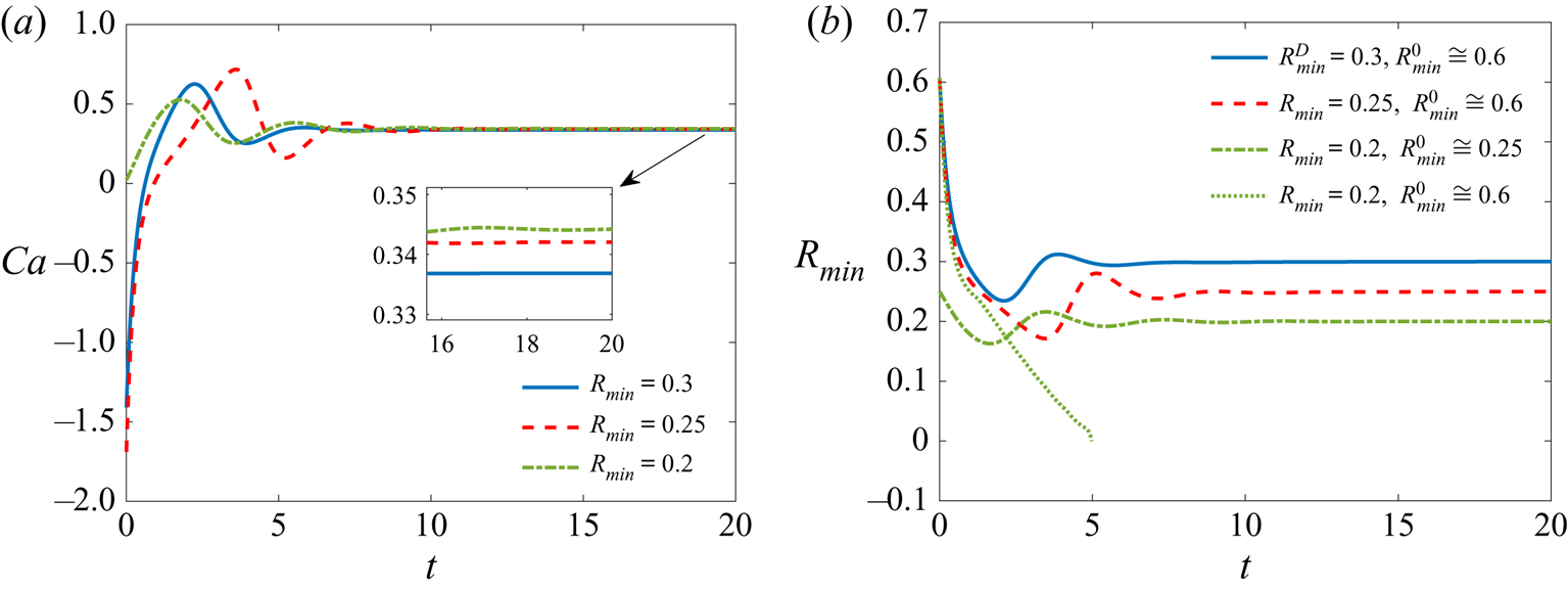
An example of the controlled dynamics is presented in figure 4. The control was designed for  $Ca_0 = 0.3$ and
 $Bo = -4$, for which
 $R_{min,0}=0.6$. The corresponding stationary shape has
 $R_{min,0} \simeq 0.6$. The gains were chosen as
 $K_p=5.565$ and
 $K_I=1.553$ (see (4.8)). Figures 4(a) and 4(b) show the dynamics of
 $Ca$ and
 $R_{min}$, respectively. Solid blue, dashed red and dotted green curves are computed starting with the same initial shape (stationary shape from Malik et al. (Reference Malik, Lavrenteva and Nir2021)), corresponding to
 $Ca_0 = 0.3, Bo = -4$ and aiming to
 $R_{min}^D=0.3,~0.25$ and
 $0.2$, respectively.
Effect of flow control on (a)  $Ca$ and (b)
 $R_{min}$ in the case of
 $Bo=-4$ for
 $R_{min}=0.3, 0.25$ and
 $0.2$ when
 $K_p=5.565$ and
 $K_I=1.553$.

Evidently, the dynamics begins with  $R_{min}=0.6$ and the modification in
 $Ca(t)$ corrects
 $R_{min}(t)$ with a fast rise time in a manner to minimize the error between the calculated and the desired
 $R_{min}$ values. In the cases described by the dashed red and solid blue lines, figure 4(a) shows that, with a slight overshoot, the
 $Ca(t)$ settles down quickly and stabilizes to
 $Ca$ values (i.e.
 $Ca^D$) that maintain
 $R_{min}^D$ as depicted in figure 4(b). However, the initial shape that was used for obtaining
 $R_{min}^D=0.3$ and
 $0.25$ fails to generate a stabilized drop with
 $R_{min}^D=0.2$ (dotted green curve in figure 4b). Hence, in this case, the last obtained stationary shape of
 $R_{min}^D=0.25$ and the corresponding
 $Ca_0=0.3421$ were used in (5.1), which served well as an initial condition for stabilizing the drop shape with
 $R_{min}^D=0.2$ (see dashed–dotted green curve). Note that for the case
 $R_{min}^D=0.25$, the overshoot as well as the settling time are relatively higher when compared with the other two cases, because the initial shape in this case is relatively far away from the desired shape.
The example described above and illustrated in figure 4 is a typical one: a control, designed on the basis of the two-state model for a given pair  $(Bo, Ca_0)$, corresponding to a stationary shape with
 $R_{min,0}$, when applied to a full system with this very stationary shape as initial condition, converges to a stationary solution with
 $R_{min}^D \in U(R_{min,0})$, i.e. in some vicinity of
 $R_{min,0}$. When using the same initial stationary state fails to generate the new desired shape, we use the last obtained stationary shape of the stabilized drop as the initial shape for simulation with the same controller gain values.
Note that the instability in drop shape develops faster with increase in the external flow velocity (proportional to  $Ca$) in any particular case of
 $Bo$. For instance, in the previous discussed example with
 $Bo=-4$, the positive eigenvalue of (4.2) for
 $Ca=0.33683$ and
 $R_{min}=0.3$ is
 $\lambda _{0.33683}=0.6514$, while for
 $Ca=0.34424$ and
 $R_{min}=0.2$ it moves to
 $\lambda _{0.34424}=0.8099$. The stabilization of such ‘more unstable’, i.e. faster diverging, shapes may not be attained with the previously designed controller and is likely to require higher controller gains. At this point, we design a new controller for the updated stationary values corresponding to the new
 $Ca$, if available, according to Malik et al. (Reference Malik, Lavrenteva and Nir2021). If no such stationary drops are available, we design a new controller based on the shape and
 $Ca$ of the previously stabilized drops. The simulation and stabilization of drops for neighbouring flow conditions are performed considering this new stationary shape. With the help of the procedure described above we succeeded to obtain stationary shapes close to collapsed torus with
 $R_{min}$ as small as
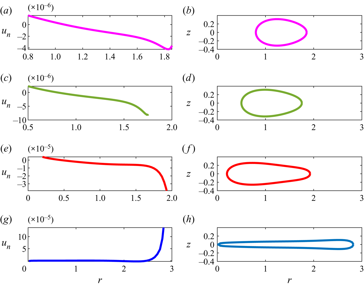
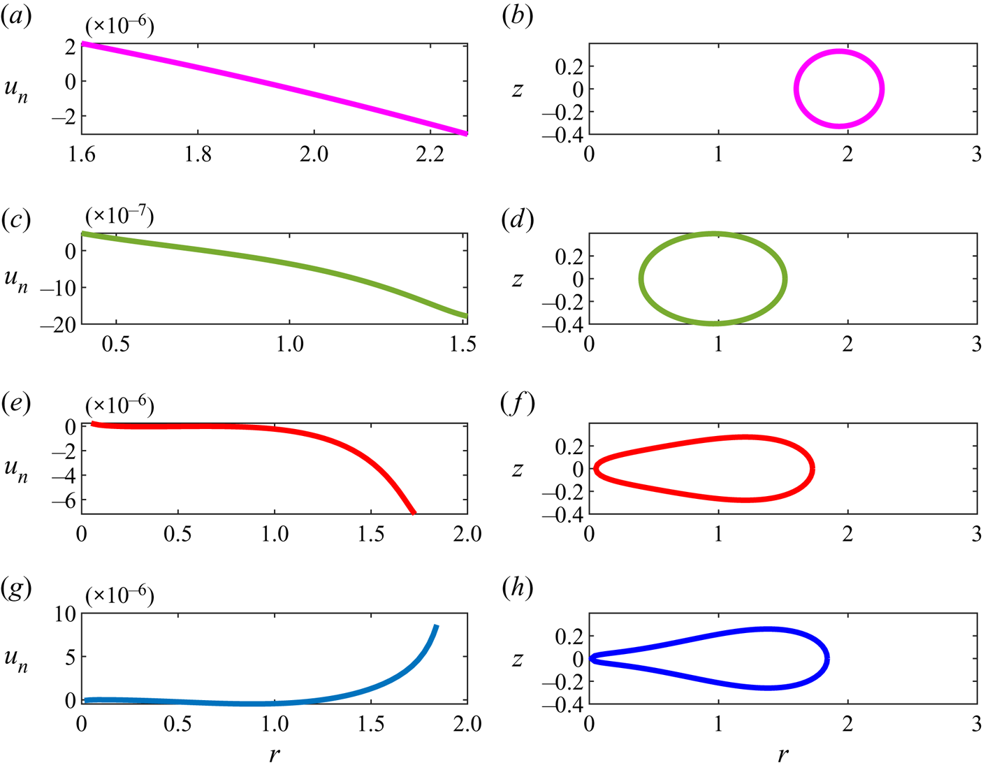
 $0.01$. Examples of the such obtained stationary shapes are presented in figures 5 and 6.
Shape and surface normal velocity component of rotating drops in compressional flow for  $Bo=-4$, (a,b)
 $R_{min}=0.8$,
 $Ca=0.27976916$, (c,d)
 $R_{min}=0.5$,
 $Ca=0.31127767$, (e,f)
 $R_{min}=0.2$,
 $Ca=0.34421500$, (g,h)
 $R_{min}=0.018$,
 $Ca=0.30130048$.

Shape and surface normal velocity component of rotating drops for  $Bo=1$, (a,b)
 $R_{min}=1.6$,
 $Ca=-0.00835739$, (c,d)
 $R_{min}=0.4$,
 $Ca=0.08147335$, (e,f)
 $R_{min}=0.05$,
 $Ca=0.14607473$, (g,h)
 $R_{min}=0.015$,
 $Ca=0.14244529$.

Figure 4 signifies that, on implementing the control,  $R_{min}$ reaches
 $R_{min}^D$ after the dynamic modification in
 $Ca$ as in (5.1). To verify that in fact the drops are stabilized and a stationary solution of the nonlinear system was found, we presented the normal velocity,
 $u_n$, at the interface of the drop cross-sections in figures 5(a,c,e,g) and 6(a,c,e,g). Those plots show that
 $u_n$ is maintained in the order of
 $10^{-5}$, or less, throughout the study. The maximum value of normal velocity is always found near
 $R_{max}$. The cross-section shapes of the corresponding stabilized drops are presented in figures 5(b,d,f,h) and 6(b,d,f,h).
Recall, from (2.8), that  $Bo<0$ represents drops with lesser density than that of the surrounding fluid. In figure 5, where the drop is lighter, the rotation coupled with higher flow velocity, i.e. higher
 $Ca$, reshapes the drop towards collapse (on the
 $z$-axis). Here, the shear counteracts this effect and, therefore, is relatively high, increasing with decrease of
 $R_{min}$. The stationarity is achieved with an increase of the curvature at
 $R_{max}$, the outer region. As a result, shown in figure 5(b,d,e,g), the egg shapes point outward except when the drop is almost collapsed. In figure 6, where the drop is heavier, the phenomenon is different. Here, both rotation and compression act in the same direction, i.e. to expand the torus outward (except in figure 6b where the flow is extensional and the cross-section is almost circular). At stationarity, the
 $Ca$ is relatively lower, compared with figure 5, and the egg shapes exhibit the pointed side towards the
 $z$-axis where the high curvature counteracts the expanding action of rotation and compression.
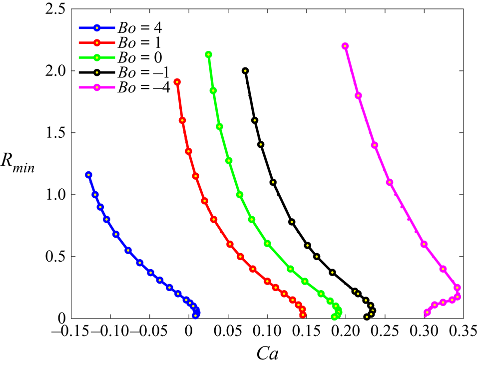
An interesting phenomenon, that is evident in all cases of  $Bo$ considered in this paper, can be seen in figure 7: there is a maximal value of
 $Ca$ beyond which no stationary tori were observed. A decrease in
 $Ca$, towards the point of collapse, occurs in spite of the monotonic decrease in
 $R_{min}$. Moreover, in the region
 $Ca$(collapse)
 $< Ca < Ca_{max}$, there are two different stationary solutions associated with different shapes, different
 $R_{min}$ and deformation factor
 $D$ values, for given
 $Ca$ and
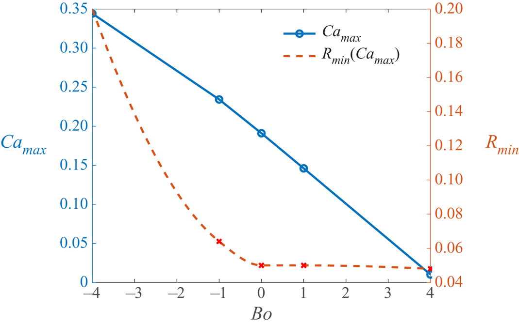
 $Bo$ (see figure 7). A summary of this is depicted in figure 8, where
 $Ca_{max}$ and
 $R_{min}(Ca_{max})$ are shown versus
 $Bo$ in the region
 $-4 < Bo < 4$.
The  $R_{min}$ values of stationary drops for various
 $Bo$ and
 $Ca$.

Variation of  $Ca_{max}$ and
 $R_{min}(Ca_{max})$ with
 $Bo$.

In all cases of  $Bo$, the reduction of
 $R_{min}$ beyond the points corresponding to
 $Ca_{max}$ yield increasingly faster diverging instabilities, requiring ever increasing controller gains
 $K_p$ and
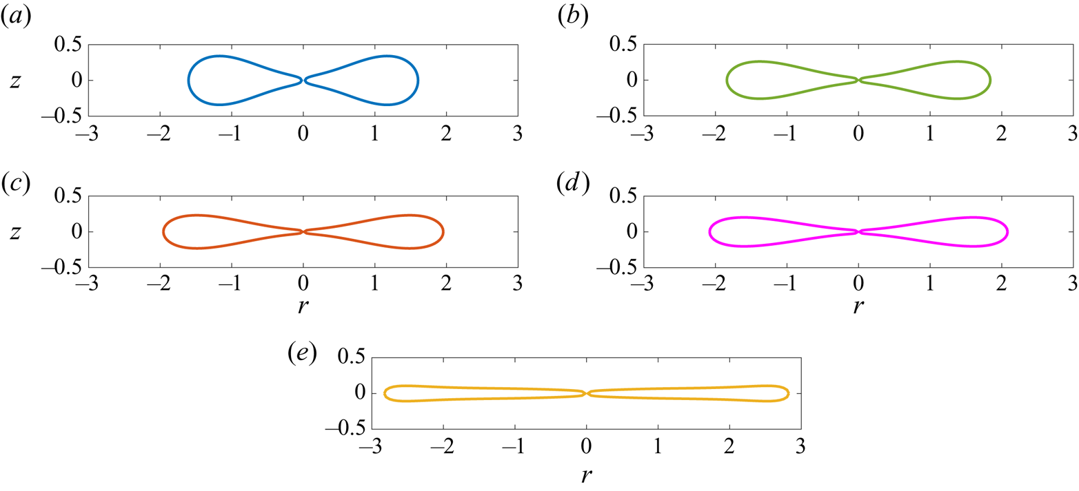
 $K_I$. Figure 9(a–e) depicts the cross-sectional shapes of toroidal drops just before the collapse state for
 $Bo=4$,
 $1, 0 ,-1$ and
 $-4$ with
 $R_{min}=0.023$,
 $0.015$,
 $0.013$,
 $0.013$ and
 $0.018$, respectively. These shapes are the last stabilized shapes before collapse that were obtained using the discussed control approach. Beyond these shapes, the encountered instabilities cannot be stabilized using current control method, even with very high gain values. The cross-sections in figure 9 indicate that the instabilities develop faster when density difference between drop and outer fluid is higher. Thus, the stabilization in the cases of
 $Bo=4$ and
 $-4$ were limited only down to
 $R_{min}=0.023$ and
 $R_{min}=0.018$ whereas, when this density difference is lower, i.e.
 $Bo=1, 0$ and
 $-1$, the drop can be stabilized down to
 $R_{min}=0.013$. Moreover, the collapsing drop thickness at these extreme points changes monotonically. At
 $Bo=-4$, where both rotation and shear tend to drive the torus to expand, the cross-section is slender with an almost negligible thickness. With the increase in
 $Bo$, the thickness of the toroidal drop cross-section increases continuously due to its increasing density as compared with outer fluid and the change of the flow from compressional to extensional.
Shapes of deformed tori near total collapse for (a)  $Bo=4, Ca=0.00842788, R_{min}=0.23$, (b)
 $Bo=1, Ca=0.14244529, R_{min}=0.015$, (c)
 $Bo=0, Ca=0.18558533, R_{min}=0.013$, (d)
 $Bo=-1, Ca=0.22686352, R_{min}=0.013$ and (e)
 $Bo=-4, Ca=0.30130048, R_{min}=0.018$.

Figure 10 depicts the stationary Taylor deformation factor for  $Bo=4, 1, 0, -1$ and
 $-4$, which contain the primary results of this work. The dashed lines represent the stable solutions, which exist only in the case of extensional flow (Malik et al. Reference Malik, Lavrenteva and Nir2021). Each of these curves contain two major sections, that demonstrates the power of superimposing a control procedure with the numerical fluid mechanics process. The solid curves represent the numerical solutions, reported in Malik et al. (Reference Malik, Lavrenteva and Nir2021). These deformations were stationary, yet unstable. Superimposed on the curves are points, shown as circles, of results of the present calculations showing stabilization of the numerically calculated shapes by imposing the control procedure. Beyond these curves we depict results, obtained in this study, presenting stabilized stationary solutions that were not reported before. These are shown in small dotted lines that approach
 $Ca_{max}$ for each
 $Bo$ case and beyond, up to an almost total collapse.
Stabilized stationary deformation curves for various  $Bo$ and
 $Ca$. Circles denote current results. Dotted and solid curves denote the newly obtained results and those previously calculated by numerical calculation, respectively. Dashed curves denote stable results of Malik et al. (Reference Malik, Lavrenteva and Nir2021). Large circles are results present in figures 5, 6 and 11.

6. Conclusions and discussion
Classical feedback control methods were employed to stabilize toroidal drops in the linear flow. As a control signal, we chose the intensity of the axisymmetric (non-rotational) component of the outer flow,  $Ca$. The control was designed using a simplified two-state dynamic model and applied on the full state dynamic equations of the drop deformations. We succeeded in stabilizing all the unsteady stationary toroidal shapes obtained previously. Moreover, the dynamic control scheme enabled the construction of new shapes – almost collapsed, highly unstable tori – that could not be previously obtained via direct numerical calculation. Thus, the obtained algorithm can be considered as an iteration method that converges to stationary shapes of toroidal drops in linear flow.
The stationary drops, once obtained with the help of designed control algorithm, can be solidified, for example, by cross-linked polymerization and form toroidal microparticles. The non-spherical microparticles, similar to the ones studied in the current study, may be potentially used as building blocks for self-assembled materials including clustering of cells, imaging probes for therapy, drug carriers as mentioned in Malik et al. (Reference Malik, Lavrenteva and Nir2021) and the studies cited therein.
It is interesting to compare the accuracy and efficiency of this method with ones used previously to obtain such solutions. Since, for stationary shapes, the normal velocity component at the interface equals zero, we use this normal velocity to characterize the accuracy of the obtained solutions.
A method employed in a series of works (Zabarankin et al. Reference Zabarankin, Smagin, Lavrenteva and Nir2013, Reference Zabarankin, Lavrenteva and Nir2015; Ee et al. Reference Ee, Lavrenteva, Smagin and Nir2018; Banerjee et al. Reference Banerjee, Lavrenteva, Smagin and Nir2021; Malik et al. Reference Malik, Lavrenteva and Nir2021) was to simulate dynamic deformations and search for initial conditions that lead to a vicinity of a stationary shape. This method requires multiple runs of a solver to obtain a single solution. Nevertheless, it proved to be effective to extended toroidal shapes at low values of  $Ca$ with a sufficient degree of accuracy. However, with increase of
 $Ca$, the accuracy and the efficiency decreases. Moreover, this method fails to find shapes of almost collapsed tori, the existence of which was anticipated from the analogy with a related problem of rotating drops (Fontelos et al. Reference Fontelos, García-Garrido and Kindelán2011).
Another method to approximate a stationary shape of the drop is to consider a family of shapes, depending on a finite number of parameters, and to minimize some norm of the interfacial normal velocity. In the application to toroidal drops, this approach was discussed in Zabarankin et al. (Reference Zabarankin, Lavrenteva and Nir2015). Lavrenteva et al. (Reference Lavrenteva, Ee, Smagin and Nir2021) considered a three-parameters family of axisymmetric bodies, with cross-sections of generalized Cassini ovals, and obtained branches of stationary shapes of singly connected and toroidal drops embedded in axisymmetric biextensional flow. This method requires finding a minimum of a function of several real variables and, thus, it is highly effective. However, the accuracy of the obtained solutions depends on how the real shapes can be approximated by the ones of the chosen family, while the accuracy of the method used in this work is limited solely by the accuracy of the solver, which in the present case was based on the boundary elements technique with only 100 elements at the interface and can easily be improved by refining the number of elements.
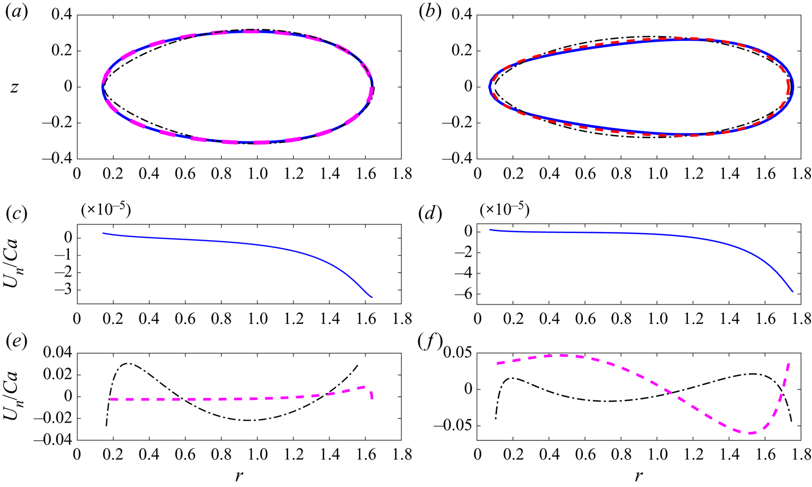
The comparison of shapes and interfacial normal velocities obtained by the three methods for  $Bo = 0, \ Ca =0.18$ and
 $Ca =0.19$ is presented in figure 11, respectively. Solid, dashed and dashed–dotted lines present the results of the method of this paper, Zabarankin et al. (Reference Zabarankin, Lavrenteva and Nir2015) and (Lavrenteva et al. Reference Lavrenteva, Ee, Smagin and Nir2021), respectively. One can see that the shapes obtained by simulating controlled and uncontrolled dynamics are almost indistinguishable, while the normal velocity obtained by the method of this paper is two to three orders of magnitude lower. Note that the papers mentioned above use a different velocity scale,
 $b G=U^* Ca$ and we compare the velocity scaled as in Zabarankin et al. (Reference Zabarankin, Lavrenteva and Nir2015). Generalized Cassini ovals approximation gives similar shapes, yet with some minor deviations, and the normal velocity is of the same order of magnitude as the method of Zabarankin et al. (Reference Zabarankin, Lavrenteva and Nir2015). For smaller values of
 $Ca$, the accuracy of all the methods improves and the difference in shapes decreases dramatically (see Lavrenteva et al. Reference Lavrenteva, Ee, Smagin and Nir2021).
A comparison of cross-section shapes and normal velocity components of stationary toroidal drops. Solid, dashed and dashed–dotted shapes show stabilized (controlled), unstable (numerical calculation (Malik et al. Reference Malik, Lavrenteva and Nir2021)) and approximated (generalized Cassini ovals (Lavrenteva et al. Reference Lavrenteva, Ee, Smagin and Nir2021)), respectively. (a) Here  $Bo = 0$,
 $Ca = 0.18$ in all cases and (b)
 $Bo =0, Ca = 0.19$. Here stabilized (controlled) results correspond to
 $Ca = 0.1904$.

In the present study we focused on microdrops, where the effects of inertia and gravity are negligibly small as addressed in Fontelos et al. (Reference Fontelos, García-Garrido and Kindelán2011) and Malik et al. (Reference Malik, Lavrenteva and Nir2021). For larger drops, these effects become more important and attract the attention of many investigators. Several studies are available in the literature on the effect of inertia in the problem of flow induced slender drop deformations (see Sangli, Riaz & Bigio (Reference Sangli, Riaz and Bigio2021) and the literature cited therein) and in the problem of drop deformation under electric field (Lanauze, Walker & Khair Reference Lanauze, Walker and Khair2013). The results of these show that the presence of inertia is especially important for the dynamics and stability of the drops.
To conclude, the method of controlled dynamics developed in this paper proved to be highly effective and accurate in constructing unstable stationary shapes of a drop in linear flow and can be used to obtain unstable stationary drop shapes in various other types of outer flow and geometry of the interface such as liquid bridges, jets, sessile or pendent drops, and others. Also, the effects of inertia can be taken into account and the drop deformation in the presence of various body forces such as gravity and electric or magnetic fields can be tackled using this approach.
Funding
This work was supported in by the Israel Science Foundation (grant ISF 1207/18). O.M.L. also acknowledges the support of a joint grant from the Center for Absorption in Science of the Ministry of Immigrant Absorption and the Committee for Planning and Budgeting of the Council for Higher Education under the framework of the KAMEA Program.
Declaration of interests
The authors report no conflict of interest.