1. Introduction
The interaction between fluid flow and flexible plates is prevalent in natural environments and industrial applications. To name a few instances, such as the biological locomotion of fish fins (Gazzola, Argentina & Mahadevan Reference Gazzola, Argentina and Mahadevan2014; Lauder Reference Lauder2015) and insect/bird/bat wings (Bomphrey et al. Reference Bomphrey, Nakata, Phillips and Walker2017; Cummins et al. Reference Cummins, Seale, Macente, Certini, Mastropaolo and Viola2018; Lauber, Weymouth & Limbert Reference Lauber, Weymouth and Limbert2023; Liu, Wang & Liu Reference Liu, Wang and Liu2024), the terrestrial/aquatic vegetation (Finnigan Reference Finnigan2000; de Langre Reference de Langre2008; Nepf Reference Nepf2012), the human organ tissue of vocal cords (Luo et al. Reference Luo, Mittal, Zheng, Bielamowicz, Walsh and Hahn2008, Reference Luo, Mittal and Bielamowicz2009) and heart valves (Griffith et al. Reference Griffith, Luo, McQueen and Peskin2009; Lee et al. Reference Lee, Rygg, Kolahdouz, Rossi, Retta, Duraiswamy, Scotten, Craven and Griffith2020) and heat convection enhancing devices of vortex generators (Mazharmanesh et al. Reference Mazharmanesh, Tian and Lei2023a ). The coupled fluid–structure physics can result in complex flow phenomena and structural response behaviours. In these scenarios, the orientation of the flexible plate axis relative to the flow direction plays a critical role in altering the characteristics of the fluid–structure coupling dynamic system.
One of the most frequently investigated configurations is a flexible plate aligned with the flow direction, where the clamped end of the plate is impinged by the flow, and the other end is free to move without restriction (Shelley & Zhang Reference Shelley and Zhang2011; Yu, Liu & Amandolese Reference Yu, Liu and Amandolese2019). This configuration is commonly referred to as ’conventional plate’ (Sader et al. Reference Sader, Cosse, Kim, Fan and Gharib2016a ; Huertas-Cerdeira et al. Reference Huertas-Cerdeira, Goza, Sader, Colonius and Gharib2021). When interacting with a uniform flow, the conventional plate exhibits a flapping instability. Once the flow velocity exceeds a critical value, the structural response mode switches from a stretched-straight mode into a regular limit-cycle flapping, where the flapping amplitude and frequency increase with faster flow speed (Zhang et al. Reference Zhang, Childress, Libchaber and Shelley2000). With further increasing flow velocity, a triggered chaotic flapping mode can also be observed (Alben & Shelley Reference Alben and Shelley2008). The dynamics of the flexible plate in uniform flow is the outcome of the interplay between the fluid pressure force driving the structural instability and the structural elastic force stabilising the plate (Eloy et al. Reference Eloy, Lagrange, Souilliez and Schouveiler2008). Through a comprehensive direct numerical simulation of the strong coupling between flow and flexible plate, Connell & Yue (Reference Connell and Yue2007) investigated the effect of fluid–solid mass ratio and flow viscosity on these state transitions. Inspired by the self-sustained flapping of the flexible plate immersed in the ambient flow, novel energy-harvesting devices based on the piezoelectric effect have been proposed, converting the fluid kinetic energy into structural elastic strain energy and then into electric energy, which provides a promising alternative candidate to generate electric power from renewable energy of ocean currents and waves (Allen & Smits Reference Allen and Smits2001; Lee et al. Reference Lee, Sherrit, Tosi, Walkemeyer and Colonius2015).
Noticing that the energy-harvesting capability strongly depends on the flapping amplitude of the flexible plate (Michelin & Doaré Reference Michelin and Doaré2013) and the critical flow velocity for the onset of plate self-sustained vibration (Kim et al. Reference Kim, Cossé, Ceideira and Gharib2013) is relatively high, Kim et al. (Reference Kim, Cossé, Ceideira and Gharib2013) proposed a distinctive configuration from the conventional one, where the placement of the plate is reversed, leaving the free end impinged by the flow and the clamped end downstream. This configuration is referred to as an ’inverted plate’ with respect to the uniform flow. The inverted configuration outperforms the conventional ones by
 $10^3$
times due to the increased larger internal strain, which is caused by the larger flapping amplitude and the readiness to lose structural stability (Kim et al. Reference Kim, Cossé, Ceideira and Gharib2013; Gurugubelli & Jaiman Reference Gurugubelli and Jaiman2015). More complex plate response behaviours, such as the deflected regime and the flipping regime, are discovered with varying flow speed, bending stiffness and viscous effect, which are absent in the conventional plate (Ryu et al. Reference Ryu, Park, Kim and Sung2015; Goza, Colonius & Sader Reference Goza, Colonius and Sader2018). Through experimental investigation and global stability analysis, the instability theory and physical mechanism behind the response mode transitions are studied, of which the flexible plate undergoes a static divergence instability before entering the flapping mode (Sader et al. Reference Sader, Cosse, Kim, Fan and Gharib2016a
; Goza et al. Reference Goza, Colonius and Sader2018). Moreover, Sader et al. (Reference Sader, Huertas-Cerdeira and Gharib2016b
) derived the theoretical expression of critical velocity threshold for flapping as a function of aspect ratio, and proved that a saddle-node bifurcation replaces the static divergence instability for low-aspect-ratio inverted plates (Tavallaeinejad, Païdoussis & Legrand Reference Tavallaeinejad, Païdoussis and Legrand2018).
Another commonly observed configuration in nature is a flexible plate clamped vertically in a cross-flow, either wall-mounted or freely suspended, which has attracted extensive research interest (Shelley & Zhang Reference Shelley and Zhang2011; Gosselin Reference Gosselin2019). This configuration holds a
 $90^{\circ }$
inclination angle related to the flow direction, which resembles benthic aquatic vegetation (Nepf Reference Nepf2012) or seagrass-like wave-energy harvesters deployed in coastal areas (Wang et al. Reference Wang, Liu, Wang, Wang, Wang, Zhang, Zhao, Xu and Wang2021). One of the predominant phenomena is morphological reconfiguration, where elastic bending deformation results in a reduced frontal area and a more streamlined shape (Vogel Reference Vogel1989; Alben, Shelley & Zhang Reference Alben, Shelley and Zhang2002). Consequently, the flexible plate benefits from a drag force reduction, by which the plants can improve the survival rate in a fierce flow environment (Alben et al. Reference Alben, Shelley and Zhang2002; Schouveiler & Boudaoud Reference Schouveiler and Boudaoud2006; Gosselin, de Langre & Machado-Almeida Reference Gosselin, de Langre and Machado-Almeida2010; Luhar & Nepf Reference Luhar and Nepf2011). As bending stiffness decreases, the plate can exhibit flow-induced vibrations, emerging from either a static mode or a reconfigured mode (Jin et al. Reference Jin, Kim, Fu and Chamorro2019; O’Connor & Revell Reference O’Connor and Revell2019; Chen et al. Reference Chen, Ryu, Liu and Sung2020; Zhang et al. Reference Zhang, He and Zhang2020b
). The flapping frequency of wall-mounted plates synchronises with their second natural frequency in uniform cross-flow (Zhang et al. Reference Zhang, He and Zhang2020b
; Kumar, Assam & Prabhakaran Reference Kumar, Assam and Prabhakaran2023). In addition, Pandey, Sharma & Bhardwaj (Reference Pandey, Sharma and Bhardwaj2023) numerically studied the energy-harvesting performance of a flexible plate in cross-flow and proposed optimal locations for the piezoelectric material patches, while Nové-Josserand et al. (Reference Nové-Josserand, Hebrero, Petit, Megill, Godoy-Diana and Thiria2018) investigated partially submerged flexible canopies capable of harvesting approximately half of the damped wave energy.
The literature reviewed above indicates that the inclination angle
 $\alpha$
between a flexible plate and the incoming flow plays a crucial role in determining its dynamical behaviour, including structural responses, oscillation characteristics and instability mechanisms. Despite this importance, most existing studies have primarily focused on three limiting configurations, namely
 $\alpha = 0^{\circ }$
(inverted configuration),
 $\alpha = 90^{\circ }$
(vertical configuration) and
 $\alpha = 180^{\circ }$
(conventional configuration), while systematic investigations covering intermediate inclination angles remain relatively limited. Silva-Leon & Cioncolini (Reference Silva-Leon and Cioncolini2019) investigated a clamped flexible plate with inclination angles varying from
 $\alpha = 90^{\circ }$
to
 $180^{\circ }$
reported that, although the inclination has only a minor influence on static reconfiguration, it plays a key role in selecting between large-amplitude periodic flapping and small-amplitude random vibrations. Shoele & Mittal (Reference Shoele and Mittal2016) showed that inclination effects become dominant beyond a critical angle, above which asymmetric flapping modes emerge (Tang, Liu & Lu Reference Tang, Liu and Lu2015). Focusing on moderate inclination angles, Huertas-Cerdeira et al. (Reference Huertas-Cerdeira, Goza, Sader, Colonius and Gharib2021) studied the influence of inclination on mode transition conditions. From an energy-harvesting perspective, Lim & Park (Reference Lim and Park2022) found that optimal performance is achieved in a biased flapping mode for inclination angles around
 $40^{\circ } - 45^{\circ }$
. The effect of inclination has also been explored in the context of heat transfer enhancement by flexible plates over the full range
 $0^{\circ } \le \alpha \le 180^{\circ }$
, using immersed boundary simulations for wall-mounted plates (Park Reference Park2020) and for plates suspended in a channel (Shin, Park & Shen Reference Shin, Park and Shen2022). In both cases, the optimal thermal performance is jointly governed by the structural bending stiffness and the inclination angle.
Under realistic environmental flow conditions, fluid motion is often strongly unsteady and may involve periodic flow reversal. A representative example is the wave-induced oscillatory flow experienced by aquatic vegetation in coastal regions (Méndez et al. Reference Méndez, Losada and Losada1999; Mullarney & Henderson Reference Mullarney and Henderson2010). Nevertheless, such unsteady and oscillatory flow conditions have received comparatively less attention in the studies reviewed above, which primarily focus on steady or unidirectional flows. For wind- and wave-driven energy-harvesting devices, time-varying flow direction can significantly affect harvesting performance, as observed in field measurements (Orrego et al. Reference Orrego, Shoele, Ruas, Doran, Caggiano, Mittal and Kang2017). Related studies have also examined triboelectric energy harvesters operating in coastal wave environments Wang et al. (Reference Wang, Liu, Wang, Wang, Wang, Zhang, Zhao, Xu and Wang2021). The experimental and theoretical studies on vertically clamped flexible plates in oscillatory flow by Luhar & Nepf (Reference Luhar and Nepf2016) reveal that, in addition to the conventional key parameters such as bending stiffness and flow speed, the Keulegan–Carpenter number
 ${\textit{KC}}$
and the ratio of plate length to wave orbital excursions
 $L$
representing unsteady characteristics also play a critical role in determining the fluid–structure coupling dynamics. Moreover, the frequency characteristics of plate fluttering result from the interplay between the oscillatory excitation frequency and the structural natural frequency. (Zhang & Nakamura Reference Zhang and Nakamura2024a
; Rota, Chiarini & Rosti Reference Rota, Chiarini and Rosti2025). Mazharmanesh et al. (Reference Mazharmanesh, Young, Tian, Ravi and Lai2022) and Mazharmanesh et al. (Reference Mazharmanesh, Young, Tian, Ravi and Lai2023b
) studied the energy-harvesting performance of single and dual inverted plates immersed in combined wave-current flows and focused on the effect of wave ellipticity, oscillation frequency and velocity amplitude. The energy-harvesting capability under the constructive interaction of a flexible plate group in oscillatory flow is numerically investigated (Zhu Reference Zhu2024). To fill in the knowledge gap discussed above, here, we aim to clarify the inclination effect of a flexible plate immersed in an unsteady wave-like oscillatory flow. The present work presents a numerical investigation of a two-dimensional inclined thin flexible plate subject to oscillatory flow. The effects of inclination angle, structural bending stiffness and oscillatory flow strength on the plate dynamics are examined, with particular attention to the structural response modes, plate deflection, drag force and energy conversion performance.
The remainder of this paper is organised as follows. Section 2 describes the physical problem and the mathematical formulation of an inclined thin flexible plates in oscillatory flows. In § 3, we present mesh and domain convergence studies, as well as validations of the numerical methodology for the fluid–structure interaction system. Section 4 reports the detailed results and analysis of inclined flexible plates in oscillatory flow, including structural response modes, plate deflection, drag force, vortex dynamics, the energy conversion. Finally, a summary of the conclusions can be found in § 5.
2. Physical problem and mathematical description
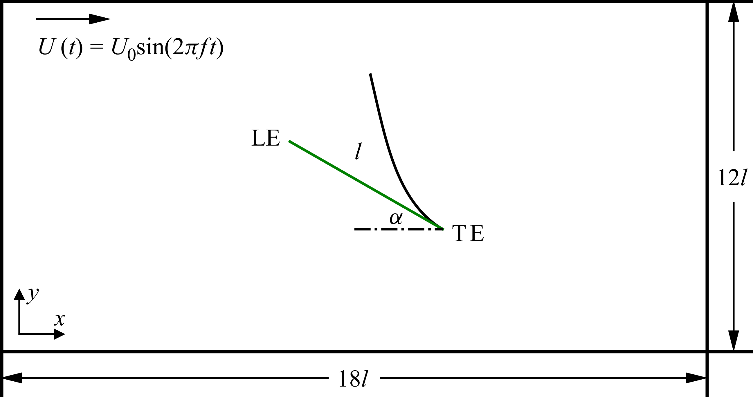
A two-dimensional model of an inclined flexible plate, as shown in the sketch in figure 1, is considered. The computational domain is an
 $18 l \times 12l$
rectangle, where
 $18 l$
and
 $12 l$
are the domain sizes along the
 $x$
and
 $y$
directions, respectively. A thin flexible plate of length
 $l$
and inclination angle
 $\alpha$
is placed in an oscillatory flow, with its trailing edge located at the centre of the computational domain. The oscillatory flow is assumed to be in the form of a sinusoidal wave with horizontal velocity written as
 \begin{eqnarray} U(t) = U_0 \textrm {sin} (2 \pi \textit{ft}), \end{eqnarray}
and vertical velocity
 $V(t) = 0$
, where
 $U_0$
is the velocity amplitude and
 $f$
is the wave frequency, giving rise to the wave orbital excursion
 $a_{w} = U_0 /(2 \pi f)$
. The velocity is set under the consideration that for a linear wave in shallow water, the velocity in the vertical component is much smaller than the horizontal one (Dean & Dalrymple Reference Dean and Dalrymple1991), which indicates that the water particle trajectory is a highly flattened ellipse, with motion dominated by back-and-forth oscillations in the horizontal direction. The prescribed flow velocity condition is accomplished by adding an oscillating pressure gradient term in the momentum equations. The trailing edge of the plate is fixed and clamped with an inclination angle
 $\alpha$
, while the leading edge of the plate is set to move freely. The boundary conditions of the computational domain are free-slip conditions at the top and bottom boundaries and periodic conditions at the left- and right-hand boundaries.
Sketch of an inclined thin flexible plate of length
 $l$
and inclination angle
 $\alpha$
in the oscillatory flow of sinusoidal form with velocity amplitude
 $U_0$
and frequency
 $f$
. The leading edge (LE) of the plate moves freely, and the trailing edge (TE) is clamped.

The present study investigates the interaction between an oscillatory fluid flow and an inclined thin flexible plate, where the flow is considered to be incompressible and viscous. The viscous flow is governed by the incompressible Navier–Stokes equations and the continuity equation in the Eulerian coordinate system as
 \begin{align} \rho _{\!f} \left(\frac {\partial \boldsymbol u}{\partial t} + \boldsymbol u \boldsymbol{\cdot }\boldsymbol{\nabla }\boldsymbol u\right) &= -\boldsymbol{\nabla }\!p + \mu {\nabla} ^2 \boldsymbol u + \rho _{\!f} \boldsymbol g + \boldsymbol f_{\!\textit{IB}}, \end{align}
 \begin{align} \boldsymbol{\nabla }\boldsymbol{\cdot }\boldsymbol u &= 0, \end{align}
where
 $\boldsymbol u$
is the velocity,
 $p$
is the pressure,
 $\rho _{\!f}$
and
 $\mu$
are the density and the dynamic viscosity of the fluid,
 $\boldsymbol g$
is the gravity acceleration and
 $\boldsymbol f_{\!\textit{IB}}$
is the volumetric force term from immersed boundary method.
To describe the motion and deformation of the flexible plate, the nonlinear Euler–Bernoulli beam equations are employed in the Lagrangian coordinate system as (Connell & Yue Reference Connell and Yue2007; Huang, Shin & Sung Reference Huang, Shin and Sung2007)
 \begin{equation} (\rho _s - \rho _{\!f} h) \frac {\partial ^2 \boldsymbol X}{\partial t^2} = \frac {\partial }{\partial s}\left(T \frac {\partial \boldsymbol X}{\partial s}\right)-\frac {\partial ^2}{\partial s^2}\left(\textit{EI} \frac {\partial ^2 \boldsymbol X}{\partial s^2}\right) + (\rho _s - \rho _{\!f} h) \boldsymbol g + \boldsymbol F_{\!\textit{IB}}, \end{equation}
where
 $s$
is the Lagrangian coordinate along the flexible plate,
 $\boldsymbol X$
is the position of Lagrangian points on the flexible plate,
 $\rho _s$
is the structural linear mass density,
 $T$
is the tension coefficient,
 $EI$
is the bending stiffness and
 $h$
is the sectional thickness of the thin plate. Here
 $\boldsymbol F_{\!\textit{IB}}$
is the Lagrangian force exerted on the plate by the surrounding fluid.
In the present study, the plate linear density
 $\rho _s$
is assumed to be comparable to
 $\rho _{\!f} l$
. Since the sectional thickness
 $h$
is negligible relative to the plate length
 $l$
, the density difference
 $\rho _s - \rho _{\!f} h$
is approximated by
 $\rho _s$
. Furthermore, the gravitational force term is neglected in the simulations. The plate is considered to be inextensible, and the inextensibility condition is expressed by
 \begin{equation} \frac {\partial \boldsymbol X}{\partial s} \boldsymbol{\cdot }\frac {\partial \boldsymbol X}{\partial s} = 1. \end{equation}
The tension coefficient
 $T(s,t)$
is a function of both
 $s$
and
 $t$
. It is treated implicitly and determined at the intermediate time step by substituting the inextensibility constraint (2.5) into (2.4). This results in a Poisson equation for
 $T$
as follows:
 \begin{align} \frac {\partial \boldsymbol X}{\partial s} \boldsymbol{\cdot }\frac {\partial ^2}{\partial s^2}\left(T\frac {\partial \boldsymbol X}{\partial s}\right)&= \frac {1}{2} \rho _s \frac {\partial ^2}{\partial t^2}\left(\frac {\partial \boldsymbol X}{\partial s}\boldsymbol{\cdot }\frac {\partial \boldsymbol X}{\partial s}\right) - \rho _s \frac {\partial ^2 \boldsymbol X}{\partial t \partial s} \boldsymbol{\cdot }\frac {\partial ^2 \boldsymbol X}{\partial t \partial s}\nonumber\\ &\quad +\frac {\partial \boldsymbol X}{\partial s} \boldsymbol{\cdot }\frac {\partial }{\partial s} \left(\frac {\partial ^2}{\partial s^2}\left(\textit{EI}\frac {\partial ^2 \boldsymbol X}{\partial s^2}\right) - \rho _s \boldsymbol g - \boldsymbol F_{\!\textit{IB}}\right)\!. \end{align}
The obtained tension coefficient
 $T(s,t)$
at the intermediate time step is substituted into structural governing (2.4) and used as an inextensibility constraint to obtain the structure positions of each Lagrangian point at the new time step. For more details of the formulation of the above equations, one can refer to the work of Huang et al. (Reference Huang, Shin and Sung2007).
The boundary conditions of the plate at the leading edge are
 \begin{equation} T = 0, \quad \frac {\partial ^2 \boldsymbol X}{\partial s^2} = (0,0), \quad \frac {\partial ^3 \boldsymbol X}{\partial s^3} = (0,0) \end{equation}
which mean no tension force, no bending force and no shearing force acting at the free end, respectively. For the clamped boundary conditions at the trailing edge, we have
 \begin{equation} \boldsymbol X = \boldsymbol X_0, \quad \frac {\partial \boldsymbol X}{\partial s} = (\textrm {cos}\alpha , \textrm {sin}\alpha ). \end{equation}
The reference quantities, fluid density
 $\rho _{\!f}$
, plate length
 $l$
and velocity amplitude
 $U_0$
, are used to normalise the above mathematical formulations. The non-dimensional parameters are listed as follows: the ratio of the plate length to the wave orbital excursion
 $L = l/a_w$
, the Keulegan–Carpenter number
 ${\textit{KC}} = U_0/lf$
, the Reynolds number
 ${\textit{Re}} = \rho _{\!f} U_0 l / \mu$
, the bending stiffness
 $K_{\!B} = EI/\rho _{\!f} U_0^2 l^3$
and the structure-to-fluid mass ratio
 $M = \rho _s/\rho _{\!f} l$
.
3. Numerical methodology and validations
Incompressible viscous flow is simulated by numerically solving the Navier–Stokes equations using the fractional-step projection method on uniform structured Cartesian meshes. The nonlinear Euler–Bernoulli beam equations are solved by the finite difference method in the Lagrangian coordinate for modelling the motion and deformation of the thin flexible plate (Huang et al. Reference Huang, Shin and Sung2007). A weak fluid–structure coupling framework is employed to couple the fluid and structure solvers, where each solver is executed once at each time step without iteration (Huang et al. Reference Huang, Shin and Sung2007).
The implicit immersed boundary method is utilised to maintain the no-slip boundary condition on the surface of the thin flexible plate and exchange the information of displacement, velocity and force among fluid Eulerian grids and structural Lagrangian points through the Dirac delta function (Mittal & Iaccarino Reference Mittal and Iaccarino2005; Griffith & Patankar Reference Griffith and Patankar2020). The volumetric force term
 $\boldsymbol f_{\!\textit{IB}}$
on the right-hand side of (2.2) is calculated by an implicit velocity correction-based immersed boundary method (Liu & Ding Reference Liu and Ding2015; Zhao et al. Reference Zhao, Chen, Yang, Liu and Shu2021) as follows:
 \begin{eqnarray} \boldsymbol f_{\textit{IB},j} = \rho _{\!f} \delta \boldsymbol u^E_j / \Delta t = \rho _{\!f} \sum _{i=1}^{l} \Delta s D_{\textit{ij}} \boldsymbol a_i, \end{eqnarray}
where
 $\delta \boldsymbol u^E_j$
is the velocity correction term acting on the intermediate fluid velocity
 $\boldsymbol u^{\ast }$
for no-slip boundary condition constraint,
 $\boldsymbol a_i$
is the feedback acceleration,
 $l$
is the number of the Lagrangian points distributed equidistantly along solid surface in the immersed boundary method,
 $\Delta s = 1.2 \Delta x$
is the arclength of the Lagrangian segments and
 $D_{\textit{ij}}$
is the weighting function in the form of
 \begin{eqnarray} D_{\textit{ij}} = \frac {1}{\Delta x \Delta y} \delta \left(\frac {x_j^E - X_i^L}{\Delta x}\right) \delta \left(\frac {y_j^E - Y_i^L}{\Delta y}\right)\!, \end{eqnarray}
where
 $\boldsymbol x_j^E = (x_j^E, y_j^E)$
and
 $\boldsymbol X_i^L = (X_i^L, Y_i^L)$
are the coordinates of Eulerian grids and Lagrangian points, respectively. The delta function
 $\delta (r)$
is in the form of a smoothed four-point piecewise function proposed in Yang et al. (Reference Yang, Zhang, Li and He2009).
The feedback acceleration
 $\boldsymbol a_i$
is the solution of the following matrix equations:
 \begin{eqnarray} \boldsymbol A \boldsymbol a = \boldsymbol b, \end{eqnarray}
with components of
 \begin{align} A_{\textit{ij}} &= \Delta s \Delta t \Delta x \Delta y \sum _{k=1}^m D_{ik} D_{\!jk}, \end{align}
 \begin{align} b_{i} &= u_i^B - \Delta x \Delta y \sum _{k=1}^m D_{ik} u_k^*, \end{align}
where
 $\Delta t$
is the time step,
 $u_k^{\ast }$
is the component of the intermediate velocity calculated by (2.2) without
 $\boldsymbol f_{\!\textit{IB}}$
. The Lagrangian force
 $\boldsymbol F_{\!\textit{IB}}$
exerted on the plate by the surrounding fluid is obtained by
 $\boldsymbol F_{\!\textit{IB}} = -\rho _{\!f} \boldsymbol a$
. Detailed discretisations of the immersed boundary method used in the present study can be found in Liu & Ding (Reference Liu and Ding2015) and Zhao et al. (Reference Zhao, Chen, Yang, Liu and Shu2021).
Numerical validation for time histories of the trailing edge lateral displacement of (a) an aligned flexible plate in a uniform flow at
 ${\textit{Re}} = 200$
,
 $K_{\!B} = 0.0015$
,
 $M = 1.5$
and
 ${\textit{Fr}} = 2.0$
with the previous literature (Huang et al. Reference Huang, Shin and Sung2007; Favier, Revell & Pinelli Reference Favier, Revell and Pinelli2014); (b) an inverted flexible plate in a uniform flow at
 ${\textit{Re}} = 250$
,
 $K_{\!B} = 0.25$
and
 $M = 1.0$
with the previous literature (Huang, Wei & Lu Reference Huang, Wei and Lu2018).

To validate the numerical methods for investigating the interaction between flow and thin flexible plates, we simulate an aligned and an inverted thin flexible plate in a uniform flow and compare the numerical results with those from the previous literature, separately. In the first validation of the aligned flexible plate, the non-dimensional parameters are
 ${\textit{Re}} = 200$
,
 $M = 1.5$
,
 $K_{\!B} = 0.0015$
and Froude number
 ${\textit{Fr}} = 2.0$
with gravitational acceleration pointing towards downstream, which are the same as those in Huang et al. (Reference Huang, Shin and Sung2007). Our numerical results of the lateral displacement of the plate trailing edge are shown in figure 2(a) in a comparison with those from the previous literature of Huang et al. (Reference Huang, Shin and Sung2007) and Favier et al. (Reference Favier, Revell and Pinelli2014). In the second validation of the inverted flexible plate, the dimensionless numbers used here are
 ${\textit{Re}} = 250$
,
 $M = 1.0$
and
 $K_{\!B} = 0.25$
, the same as those used in Huang et al. (Reference Huang, Wei and Lu2018). In figure 2(b), we show the time histories of the tip deflection of the plate in the transverse direction. Our numerical results show a good agreement with the previous literature (Huang et al. Reference Huang, Wei and Lu2018).
Numerical validation for the time series of horizontal tip positions of each flexible plate compared with experimental results of Favier et al. (Reference Favier, Li, Kamps, Revell, O’Connor and Brücker2017) and numerical results of O’Connor & Revell (Reference O’Connor and Revell2019).

Furthermore, we validate the performance of the current numerical method in modelling thin flexible plates in oscillatory flow by simulating 10 flexible flaps placed in the oscillating channel flow against experimental results (Favier et al. Reference Favier, Li, Kamps, Revell, O’Connor and Brücker2017). In the channel, the pressure gradient has a sinusoidal variation as
 $\textrm {d} p/ \textrm {d} x = A \textrm {sin} (2 \pi \textit{ft})$
, where the amplitude
 $A$
is
 $4549.13 \,{\textrm {Pa} \boldsymbol{\, }\rm m^{-1}}$
and the frequency
 $f$
is 1 Hz. The Reynolds number
 ${\textit{Re}}$
is set as 120, normalised by the maximal flow velocity in the channel without flaps. Each neighbouring stem has a horizontal gap of half of its length. The horizontal tip positions of each stem are presented in the figure 3 with those from previous experimental measurements (Favier et al. Reference Favier, Li, Kamps, Revell, O’Connor and Brücker2017) and numerical simulations (O’Connor & Revell Reference O’Connor and Revell2019). A good agreement among the results is achieved, although slight discrepancies are observed, which may arise from the difference between the two-dimensional simulations and the three-dimensional experimental settings.
Finally, the accuracy of the hydrodynamic force calculation using the present numerical method is assessed by validation against a benchmark case of a heaving flexible plate in quiescent flow. The plate is forced to heave at its leading edge with a flapping amplitude of
 $A/l = 1.2$
. The rest dimensionless parameters are
 $K_{\!B} = 0.2$
,
 $M = 1.0$
and
 ${\textit{Re}} = \rho _{\!f} U_{\textit{ref}}\, l/ \mu = 150$
, where the reference velocity is
 $U_{\textit{ref}} = 2 \pi A f$
. The time variations of drag coefficient
 $C_D = F_X / (0.5\rho U_{\textit{ref}}^2\, l)$
and lift coefficient
 $C_L = F_Y / (0.5\rho U_{\textit{ref}}^2\, l)$
in one flapping period are shown in figure 4 compared with the previous literature results (Yin & Luo Reference Yin and Luo2010; Hua, Zhu & Lu Reference Hua, Zhu and Lu2013; Xu et al. Reference Xu, Liu, Liu, Xiong and Huang2022). Our numerical results show good agreement with previous ones, thereby validating the present method. Further validation cases can be found in our previous work (Zhang & Nakamura Reference Zhang and Nakamura2024b
).
Numerical validation for time histories of (a) drag coefficient and (b) lift coefficient of a heaving flexible plate in static flow with the previous literature (Yin & Luo Reference Yin and Luo2010; Hua et al. Reference Hua, Zhu and Lu2013; Xu et al. Reference Xu, Liu, Liu, Xiong and Huang2022).

(a) The mesh independence study on tip deflection angles of case at
 ${\textit{Re}} = 200$
,
 ${\textit{KC}} = \pi$
,
 $L = 2.0$
,
 $K_{\!B} = 0.3$
and
 $\alpha = 60^{\circ }$
with four different mesh resolutions:
 $\Delta x/l$
= 1/40 (solid), 1/50 (dashed–dotted), 1/64 (dashed) and 1/80 (dotted). (b) The domain independence study on tip deflection angles of case at
 ${\textit{Re}} = 200$
,
 ${\textit{KC}} = \pi$
,
 $L = 2.0$
,
 $K_{\!B} = 0.1$
and
 $\alpha = 30^{\circ }$
with three different domain sizes:
 $12l \times 8l$
(solid),
 $18l \times 12l$
(dashed–dotted) and
 $27l \times 18l$
(dashed).

Computational mesh and domain independence studies are performed for an inclined thin flexible plate in oscillatory flows. In the simulation, the parameters are chosen as
 ${\textit{Re}} = 200$
,
 ${\textit{KC}} = \pi$
,
 $L = 2.0$
,
 $K_{\!B} = 0.3$
and
 $\alpha = 60^{\circ }$
for mesh independence test. The results of
 $\Delta x/ l = 1/40$
,
 $\Delta x/ l = 1/50$
,
 $\Delta x/ l = 1/64$
and
 $\Delta x/ l = 1/80$
are presented in figure 5(a). It is clear that the results with
 $\Delta x/ l = 1/64$
and
 $\Delta x/ l = 1/80$
are rather close, and thus,
 $\Delta x/ l = 1/64$
and
 $\Delta y/ l = 1/64$
are chosen in the following simulation. The corresponding time step is fixed to
 $\Delta t/ T = 0.0001$
. The domain independence are validated with
 ${\textit{Re}} = 200$
,
 ${\textit{KC}} = \pi$
,
 $L = 2.0$
,
 $K_{\!B} = 0.1$
and
 $\alpha = 30^{\circ }$
and the results are shown in figure 5(b) with domain size of
 $12l \times 8l$
,
 $18l \times 12l$
and
 $27l \times 18l$
. It is observed that a domain size of
 $18l \times 12l$
is sufficient to achieve accurate and convergent results, and therefore, it is adopted in the present simulation.
4. Numerical results and discussion
In this section, inclined thin flexible plates in oscillatory flow are investigated for a range of inclination angles relative to the flow direction and bending stiffness values, spanning from a rigid-like type to a highly deformable, compliant one. The range of the inclination angle is select as
 $\alpha \in [5^{\circ }, 90^{\circ }]$
and the bending stiffness is varied as
 $K_{\!B} \in [0.05, 50.0]$
. In addition, the effect of the wave strength, i.e. the wave orbital excursion, is considered and represented by the Keulegan–Carpenter number or the ratio regarding plate length.
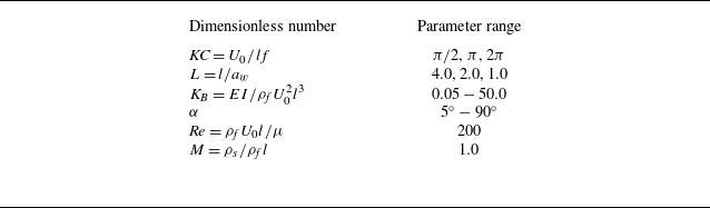
Without any special mentions, the Reynolds number is fixed to 200, and the mass ratio is fixed to 1.0 without losing any universality. The summary of the varying critical dimensionless numbers can be found in table 1.
Varying dimensionless parameters in this study.

4.1. Structural response modes
Through numerical simulations over a range of key parameters, including the dimensionless bending stiffness, the Keulegan–Carpenter number and the inclination angle, the response behaviours of a thin flexible plate in oscillatory flow can be classified into four modes: static mode, flapping mode, subharmonic flapping mode and irregular mode. The superpositions of the plate profiles together with their time histories of plate tip deflection angle and the PSD with respect to the deflection are shown in figure 6. The superposed plate profiles are plotted over four consecutive oscillatory flow periods after the plate response behaviours have reached a steady state. The tip deflection angle of the plate is measured by the straight line connecting the plate’s leading and trailing edges with respect to its initial undeformed position. The power spectra are analysed through the same time interval as that used for the deflection time histories.
Superpositions of plate profiles, tip deflection angle histories and power spectral density (PSD) for (a) static mode (
 $K_{\!B} = 4.0$
,
 ${\textit{KC}} = \pi$
and
 $\alpha = 5^{\circ }$
), (b) flapping mode (
 $K_{\!B} = 0.5$
,
 ${\textit{KC}} = \pi$
and
 $\alpha = 5^{\circ }$
), (c) subharmonic flapping mode (
 $K_{\!B} = 0.2$
,
 ${\textit{KC}} = \pi$
and
 $\alpha = 5^{\circ }$
) and (d) irregular mode (
 $K_{\!B} = 0.05$
,
 ${\textit{KC}} = \pi$
and
 $\alpha = 5^{\circ }$
).

In figure 6(a i), the static mode at a high dimensionless bending stiffness is shown, where the plate remains straight and undeformed due to the large elastic resistance against the fluid force. The temporal variation of the tip deflection angle shows a negligible deviation from zero, which is consistent with the plate profile. Multiple frequency peaks are observed for the static mode in figure 6(a iii). When the dimensionless bending stiffness decreases to
 $K_{\!B} = 0.5$
, the structural response mode switches to the flapping mode, as shown in figure 6(b i), where the plate oscillates around its equilibrium position in a regular and periodic motion with an approximately constant amplitude and frequency (see figure 6
b ii). The plate profiles over each oscillatory flow period are perfectly overlapping, and the response frequency is dominated by the external oscillatory flow frequency. The flapping mode is governed by the driven fluid pressure force and restoring elastic force, which resembles the large-amplitude flapping of an inverted flexible plate in uniform flow (Sader et al. Reference Sader, Cosse, Kim, Fan and Gharib2016a
). In figure 6(c ii), with
 $K_{\!B}$
declining to
 $0.2$
, the plate shows a similar flapping motion but with a larger flapping amplitude. However, in a single flapping period, the plate oscillates with a deflected mean position, and the mean position changes its side in two continuous periods. The switching of the mean deflected position is clearly identified from the plate profiles shown in figure 6(c i), which are distinguished by different colours. Consequently, the dominant flapping frequency is half of the oscillating flow frequency, as seen in figure 6(c iii). Therefore, in the current research, this typical structural response is referred to as the subharmonic flapping mode. Once the dimensionless bending stiffness is low enough (
 $K_{\!B} = 0.05$
), the plate flexibility is unable to provide enough resistance and resilience against the fluid force. As a result, the plate shows an irregular mode, in which the plate flapping becomes irregular and loses the periodicity as observed from figure 6(d i,d ii). The flapping frequency spectra exhibit a primary peak at the fluid oscillation frequency, accompanied by multiple subordinate peaks, particularly in the low-frequency range. The plate kinematics and flow distributions are presented in the movies provided as Supplementary material.
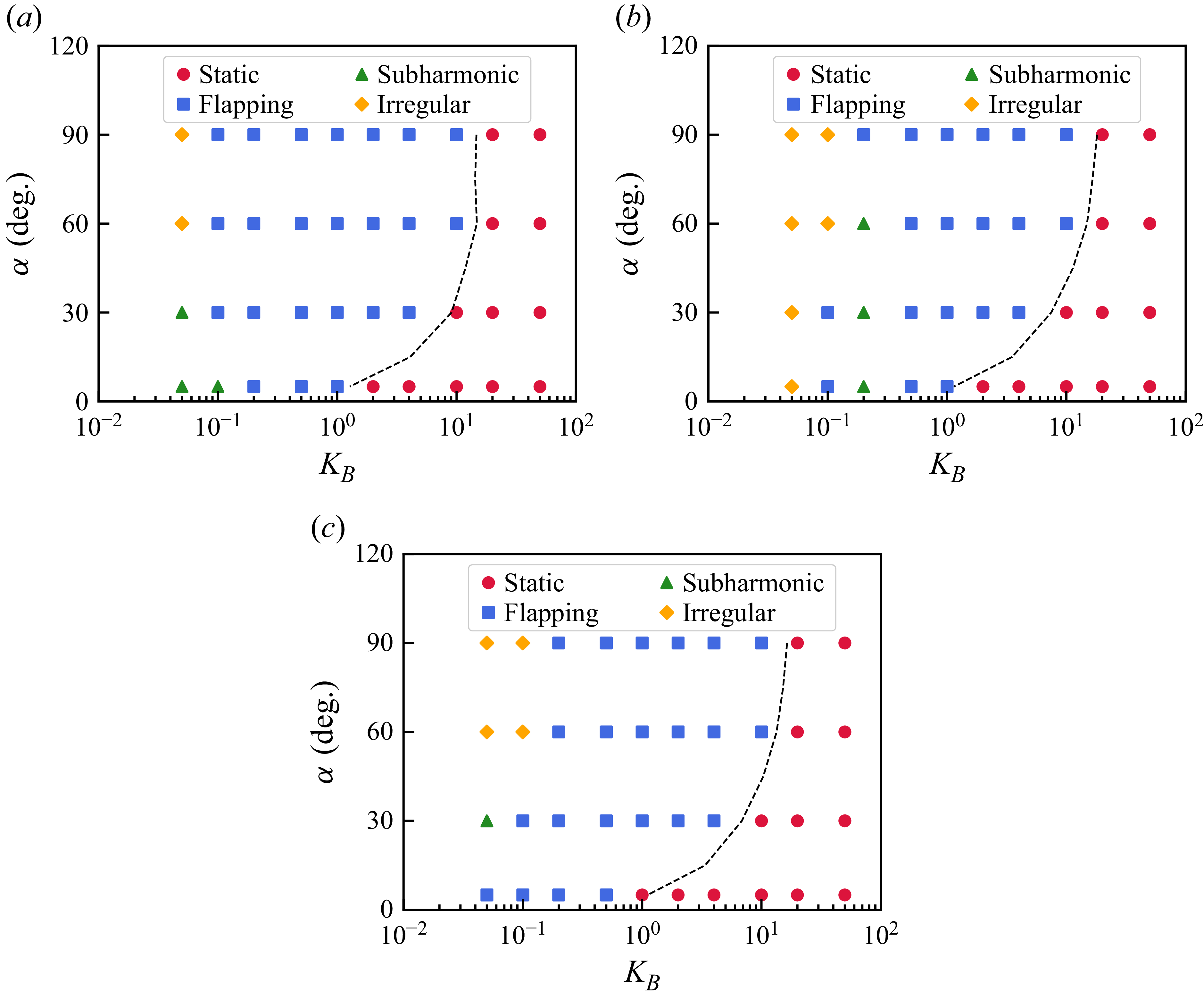
Phase diagrams of inverted plates in oscillatory flow with respect to
 $K_{\!B}$
and
 $\alpha$
under different wave orbital excursion: (a)
 ${\textit{KC}} = 2 \pi$
, (b)
 ${\textit{KC}} = \pi$
and (c)
 ${\textit{KC}} = \pi /2$
.

To investigate the variation of structural response modes of inclined thin flexible plates in oscillatory flows, we conduct a parametric sweep over the Keulegan–Carpenter number (
 ${\textit{KC}}$
), the plate flexibility (
 $K_{\!B}$
) and the inclination angle relative to the flow (
 $\alpha$
). The resulting phase diagrams in the
 $K_{\!B}$
–
 $\alpha$
plane for three representative cases,
 ${\textit{KC}} = \pi /2$
,
 $\pi$
and
 $2\pi$
, are shown in figure 7. For all three values of
 ${\textit{KC}}$
, the static mode is observed in the region of relatively large dimensionless bending stiffness
 $K_{\!B}$
. As
 $K_{\!B}$
decreases at a fixed inclination angle, a transition from the static mode to a flapping mode occurs. Furthermore, the transition boundary shifts towards higher
 $K_{\!B}$
with increasing
 $\alpha$
. This trend arises because a larger inclination angle exposes a greater frontal area to the oscillatory flow, leading to stronger pressure forces and an enhanced tendency towards static-divergence instability (Gurugubelli & Jaiman Reference Gurugubelli and Jaiman2015).
With a further decrease in bending stiffness, both subharmonic flapping mode and irregular mode emerge, depending on the parameter combinations. The subharmonic mode is confined to a very narrow range of bending stiffness, as shown in figure 7. It is worth noting that, unlike vertically wall-mounted flexible plates in oscillatory flows (Zhang & Nakamura Reference Zhang and Nakamura2024a
), for which the inclination angle relative to the flow is effectively
 $90^{\circ }$
, an inclined flexible plate does not exhibit nonlinear modes even at
 $\alpha = 90^{\circ }$
. This difference arises because the trailing edge of the inclined plate is located in an open domain, allowing the flow to shear past the plate without the confinement and ground effect induced by a nearby wall.
4.2. Vortex dynamics
For a better understanding of the interaction between the inclined flexible plates and external oscillating flow, we plot the instantaneous vorticity contour over one fluid oscillating period with varying bending stiffness for
 $\alpha = 5^{\circ }$
in figure 8 and
 $\alpha = 60^{\circ }$
in figure 9. Figure 8(a) shows the vorticity evolution for one flow period at
 ${\textit{KC}} = \pi$
,
 $K_{\!B} = 4.0$
and
 $\alpha = 5^{\circ }$
. During the rightward stroke of oscillating flow, a shear layer of positive vorticity forms on the upper surface of the plate, while a negative shear layer develops on the lower surface. After
 $t/T = 0.5$
, corresponding to flow reversal, the signs of the upper and lower shear layers switch accordingly. Owing to the small inclination angle, the shear layers remain attached to the plate surfaces throughout the oscillation cycle, without flow separation or vortex shedding. This behaviour is consistent with previous numerical studies (Gurugubelli & Jaiman Reference Gurugubelli and Jaiman2015).
Vorticity contour of inclined thin flexible plates in oscillatory flows at
 ${\textit{KC}} = \pi$
and
 $\alpha = 5^{\circ }$
with (a)
 $K_{\!B} = 4.0$
, (b)
 $K_{\!B} = 0.5$
, (c)
 $K_{\!B} = 0.2$
and (d)
 $K_{\!B} = 0.05$
. The subpanels from (i) to (iv) correspond to the different time moments
 $t/T = 0.0, 0.25, 0.5$
and
 $0.75$
, respectively. The plate kinematics and flow distributions are presented in the movies provided as Supplementary material.

Vorticity contour of inclined thin flexible plates in oscillatory flows at
 ${\textit{KC}} = \pi$
and
 $\alpha = 60^{\circ }$
with (a)
 $K_{\!B} = 4.0$
, (b)
 $K_{\!B} = 0.5$
, (c)
 $K_{\!B} = 0.2$
and (d)
 $K_{\!B} = 0.05$
. The subpanels from (i) to (iv) correspond to the different time moments
 $t/T = 0.0, 0.25, 0.5$
and
 $0.75$
, respectively. The plate kinematics and flow distributions are presented in the movies provided as Supplementary material.

In figure 8(b) of the plate at
 $K_{\!B} = 0.5$
, the plate loses the divergent stability and starts to flap under the external fluid loading. Although the general vorticity evolution is similar to the case of
 $K_{\!B} = 4.0$
(figure 8
a), the intensity of the vorticity attached to the plate surface is strengthened with a thicker shear layer. Unlike the independent development of the upper and lower shear layers at
 $K_{\!B} = 4.0$
, here a shear layer interaction is spotted. Once the left-hand stroke proceeds to the right-hand stroke, the negative vorticity filament at the leading edge is pushed rightwards and reattached to the lower surface, which merges with the lower shear layer and creates a vorticity bulge, as seen from figure 8(b ii).
When the dimensionless bending stiffness decreases to
 $K_{\!B} = 0.2$
, as shown in figure 8(c), the response mode of the plate transits to the subharmonic flapping mode, which offers a significantly larger instantaneous angle of attack due to the drastic structure deformation. Since a single structural flapping period in the subharmonic flapping mode spans two fluid oscillation periods, the illustrations shown here present only the upward flapping phase of the plate. It is clearly shown that the generated shearing vorticity layer on the plate surface is shed from the plate’s leading edge. Consequently, a vortex street consisting of pairs of vortices with opposite signs is produced along the direction of the plate’s leading edge. From the plate trailing edge, another pair of vortices of lower vorticity is shed out and dissipates in the bulk flow. For the plate of irregular mode, see figure 8(d), the extreme compliance and softness of the structure mitigate its resistance to the flow and consequent vorticity shearing. As a result, the shedding of a regular vortex street diminishes; instead, only a small vortex is produced at the plate leading edge, seen from figure 8(d iv).
Differently, for the thin flexible plate with a larger inclination angle, placed in the oscillatory flow, for instance,
 $\alpha = 60^{\circ }$
in figure 9, the vorticity evolution shows a distinctive pattern compared with the low inclination case, considering two factual differences. First, the large inclination angle causes a stronger shearing effect and flow separation. Second, a wider frontal area associated with the larger inclination angle results in a higher fluid pressure force, which drives the plate into deformation to a greater extent. Figure 9(a) shows the vorticity contour around the plate of bending stiffness
 $K_{\!B} = 4.0$
with
 ${\textit{KC}} = \pi$
and
 $\alpha = 60^{\circ }$
. Two pairs of vortex dipoles are generated and shed into the ambient flow, of which one pair is detached from the leading edge while the other comes from the trailing edge. In the right stroke, a clockwise vortex is generated and shed from the leading edge at
 $t/T = 0$
and
 $1/4$
, see figure 9(a i,a ii). However, the flow reverses its direction from right to left at
 $t/T = 1/2$
and thus pushes the shed clockwise vortex close to the plate surface. Later, the negative shear layer resulting from the strong flow shearing combines with the clockwise vortex and sheds into the bulk, forming a vortex dipole with a tight connection. It is also noted that, during vortex dipole shedding at the leading edge, a vorticity filament forms and subsequently develops into a secondary vortex of smaller scale, which then merges with the trailing edge vortex, see figure 9(a iv). For the static mode at large structural flexibility, due to the negligible degrees of freedom to plate movement, the vorticity evolution at the leading and trailing edge exhibits a highly similar processes, with only slight differences in the dipole propagation direction.
In figure 9(b), the plate response mode transitions to the flapping mode due to the reduced bending stiffness. The alignment of the bending motion with the externally driven flow mitigates the shearing effect, thereby delaying the generation of the leading edge vortex, as evidenced by a comparison between figures 9(b ii,b iii) and 9(a ii,a iii). The aligning flapping reduces the relative velocity between the structure and the bulk flow; therefore, as shown in figure 9(b iv), only a vorticity filament is shed from the leading edge instead of a fully developed vortex, which is caused by the reduced flow shearing. The vorticity filament subsequently grows into an anticlockwise vortex, which further spreads into the far field, accompanied by the clockwise vortex from the last stroke. At the trailing edge of the plate at
 $K_{\!B} = 0.5$
, although the vorticity filaments of both signs detach from the plate due to the sharp edge, no complete vortices are spotted since the filament either merges with the shear layer at the plate surface or dissipates in the background flow. In figure 9(c), for the case of
 $K_{\!B} = 0.2$
, the vorticity evolution pattern reverses compared with the
 $K_{\!B} = 0.5$
case, where the shedding of vortex pairs occurs only at the trailing edge. The upper part of the plate suffers a slighter flow shear and separation due to the large deformation under lower flexibility. A similar vorticity contour can be found in figure 9(d) for the irregular mode, even under a chaotic and aperiodic structural response.
4.3. Lift coefficients of rigid plates in oscillatory flow
The interaction between the flexible structure and the background flow, particularly the associated structural response behaviours, is governed by the balance between external fluid loading and internal structural restoring forces arising from flexibility. The fluid force depends strongly on the relative velocity, frontal area and drag and lift coefficients, which are in turn determined by the structural shape and its degree of streamlining. In this section, we derive the variations of the force coefficients for rigid plates with different inclination angles in oscillatory flow.
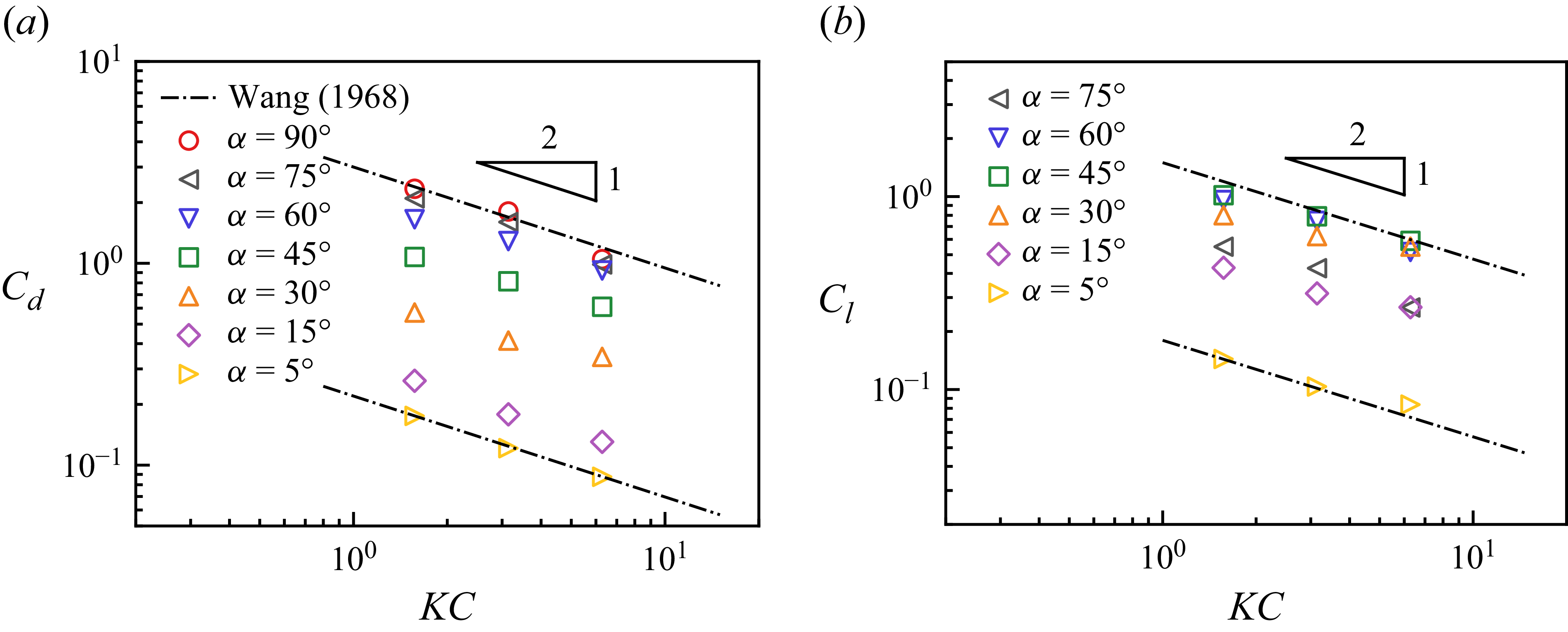
(a) Drag coefficients
 $C_d$
and (b) lift coefficients
 $C_l$
of inclined rigid plates in oscillatory flows under various Keulegan–Carpenter numbers,
 ${\textit{KC}}$
, and inclination angles,
 $\alpha$
.

For rigid structures immersed in oscillatory flow, extensive experimental and theoretical studies have been conducted on cylinders and vertical plates (Keulegan & Carpenter Reference Keulegan and Carpenter1958; Wang Reference Wang1968). The drag coefficients of a rigid structure immersed in oscillatory flow can be expressed as follows:
 \begin{equation} C_d = \frac {3}{4} \int _{0}^{2\pi } \frac {F_d \textrm {cos} \theta }{\rho _{\!f} U_0^2 l} \textrm {d} \theta , \end{equation}
where
 $F_d$
is the horizontal component of the hydrodynamic force exerted on the plate and
 $\theta$
is the instantaneous phase. Figure 10(a) shows the calculated drag coefficients by (4.1) as a function of
 ${\textit{KC}}$
with varying inclination angles. As the inclination angle increases, the drag coefficient increases in value, as the plate exposes a wider frontal area and receives higher fluid loading. For the wall-mounted immersed structure in the oscillatory flow, the variation of the drag coefficient follows the scaling law as
 $C_d \sim KC^{-1}Ro^{-1/2}$
(Keulegan & Carpenter Reference Keulegan and Carpenter1958; Zhang & Nakamura Reference Zhang and Nakamura2024a
), where
 $Ro = \rho _{\!f} l^2 f / \mu$
is the Roshko number (Williamson & Brown Reference Williamson and Brown1998). On the other hand, when the structure undergoes the oscillatory flow effect in an open domain, the variation of the drag coefficient follows the scaling law of
 $C_d \sim KC^{-1/2}Re^{-1/2}$
(Keulegan & Carpenter Reference Keulegan and Carpenter1958). As shown in figure 10(a), under the fixed viscous effect
 ${\textit{Re}} = 200$
, the drag coefficient is proportional to the inverse square root of
 ${\textit{KC}}$
,
 $C_d \sim KC^{-1/2}$
for each inclination angle, which is consistent with the previous research results.
However, in previous studies (Keulegan & Carpenter Reference Keulegan and Carpenter1958; Wang Reference Wang1968), only expressions for the drag coefficient were derived, as these works focused on cylinders or vertical plates. Owing to their geometric symmetry with respect to the flow direction, such configurations theoretically generate no lift force. When a plate is placed in oscillatory flow at a finite inclination angle
 $\alpha \ne 0^{\circ }$
and
 $\alpha \ne 90^{\circ }$
, a lift force arises naturally due to the broken symmetry, with its direction changing in association with flow reversal. To quantitatively describe the effect of inclination on the lift force, we derive the lift coefficient of an inclined rigid plate in oscillatory flow to characterise the lift force variation.
First, we consider the instantaneous lift force acting on a plate with an angle of attack
 $\alpha$
(i.e. the inclination angle) in a uniform flow with fluid velocity
 $U$
. The lift force can be expressed as
 \begin{equation} F_l = \frac {1}{2} \rho _{\!f} l C_l (\alpha ) U(t)|U(t)|. \end{equation}
Once we substitute the velocity profile of the oscillatory flow,
 $U(t) = U_0 \textrm {cos} (2 \pi ft)$
, into (4.2), we can have the dimensionless instantaneous lift force within oscillatory flow as
 \begin{equation} \frac {F_l}{\rho _{\!f} U_0^2 l} = \frac {C_l}{2}|\textrm {cos}\theta |\textrm {cos}\theta , \end{equation}
where
 $\theta$
is the instantaneous phase,
 $\theta = 2 \pi \textit{ft}$
.
Note that the lift force exhibits half-period antisymmetry, as once the oscillatory flow reverses from the right-hand stroke to the left-hand stroke, the direction of the lift force changes from upwards to downwards. Owing to the flow symmetry, the lift force satisfies the following relation:
 \begin{equation} F_l(\theta ) = -F_l(\theta +\pi ). \end{equation}
For the half-period antisymmetric function, using Fourier series expansion, we can have
 \begin{align} \frac {F_l}{\rho _{\!f} U_0^2 l} &= A_1\textrm {sin}\theta + A_3\textrm {sin}3\theta + A_5\textrm {sin}5\theta + \ldots \nonumber\\ &\quad + B_1\textrm {cos}\theta + B_3\textrm {cos}3\theta + B_5\textrm {cos}5\theta + \ldots , \end{align}
where the coefficients in the Fourier series expansion are
 \begin{equation} A_n = \frac {1}{\pi } \int _{0}^{2 \pi } \frac {F_l \textrm {sin} n\theta }{\rho _{\!f} U_0^2 l} \textrm {d} \theta , \end{equation}
and
 \begin{equation} B_n = \frac {1}{\pi } \int _{0}^{2 \pi } \frac {F_l \textrm {cos} n\theta }{\rho _{\!f} U_0^2 l} \textrm {d} \theta . \end{equation}
On the other hand, the expression
 $|\textrm {cos}\theta |\textrm {cos}\theta$
can be expanded by Fourier series as
 \begin{equation} \begin{aligned} |\textrm {cos}\theta |\textrm {cos}\theta & = \sum _{n=0}^{\infty } \frac { \displaystyle \int _{0}^{2 \pi } |\textrm {cos}\theta |\textrm { cos}\theta \textrm {cos}n\theta \textrm {d}\theta }{\displaystyle \int _{0}^{2 \pi } \textrm {cos}^2 n\theta \textrm {d}\theta } \\ & = a_0 + a_1\textrm {cos}\theta + a_2\textrm {cos}2\theta + a_3\textrm {cos}3\theta + \ldots , \end{aligned} \end{equation}
where
 \begin{equation} a_n = 0 \; \textrm {for} \; n \; \textrm {is} \; \textrm {even}, \end{equation}
and
 \begin{equation} a_n = (-1)^{\frac {n+1}{2}}\frac {8}{n(n^2-4)\pi } \; \textrm {for} \; n \; \textrm {is} \; \textrm {old}, \end{equation}
therefore,
 \begin{equation} a_1 = \frac {8}{3\pi }, \; a_3 = \frac {8}{15\pi }, \; a_5 = -\frac {8}{105\pi }, \; \ldots . \end{equation}
Introducing the Fourier series expansion of term
 $|\textrm {cos}\theta |\textrm {cos}\theta$
, (4.8), into (4.5) and collecting the terms of the same trigonometric functions in the Fourier series expansion with the coefficients rearranged as
 \begin{equation} \left \{ \begin{aligned} B_1^{\prime } &= \frac {B_1}{a_1}, \\ B_3^{\prime } &= B_3 - B_1\frac {a_3}{a_1}, \\ B_5^{\prime } &= B_5 - B_1\frac {a_5}{a_1} \ldots , \end{aligned} \right . \end{equation}
we can have
 \begin{align} \frac {F_l}{\rho _{\!f} U_0^2 l} & = A_1\textrm {sin}\theta + A_3\textrm {sin}3\theta + A_5\textrm {sin}5\theta + \ldots \nonumber\\ &\quad + B_1^{\prime }|\textrm {cos}\theta |\textrm {cos}\theta + B_3^{\prime }\textrm {cos}3\theta + B_5^{\prime }\textrm {cos}5\theta + \ldots . \end{align}
Consequently, it can be written as
 \begin{align} \frac {C_l}{2} & = B_1^{\prime } + \frac {B_3^{\prime }\textrm {cos}3\theta }{|\textrm {cos}\theta |\textrm {cos}\theta } + \frac {B_5^{\prime }\textrm {cos}5\theta }{|\textrm {cos}\theta |\textrm {cos}\theta } + \ldots \nonumber\\ &\quad + \frac {A_1\textrm {sin}\theta }{|\textrm {cos}\theta |\textrm {cos}\theta } + \frac {A_3\textrm {sin}3\theta }{|\textrm {cos}\theta |\textrm {cos}\theta } + \frac {A_5\textrm {sin}5\theta }{|\textrm {cos}\theta |\textrm { cos}\theta } + \ldots . \end{align}
Since the lift coefficient is required to be phase-independent over a single oscillation period, all coefficients multiplying the trigonometric function terms must vanish. Hence, the lift coefficient of an inclined rigid plate in oscillatory flow can be expressed as
 \begin{equation} C_l = 2B_1^{\prime } = \frac {3}{4} \int _{0}^{2 \pi } \frac {F_l \textrm {cos} \theta }{\rho _{\!f} U_0^2 l} \textrm {d}\theta . \end{equation}
In figure 10(b), the lift coefficients are plotted as functions of the Keulegan–Carpenter number for different inclination angles
 $\alpha$
. The lift coefficient depends on
 $\alpha$
through both the exposed frontal area and the force decomposition induced by the inclination. Similar to the drag coefficient, the lift coefficient exhibits a scaling law with the Keulegan–Carpenter number as
 \begin{equation} C_l \sim KC^{-1/2}. \end{equation}
The lift coefficient,
 $C_l$
, initially increases with the inclination angle
 $\alpha$
, reaches a maximum at
 $\alpha = 45^{\circ }$
, and then decreases monotonically. Since the plate at
 $\alpha = 90^{\circ }$
has a symmetry shape with respect to the incoming flow, the resulting lift coefficient is negligibly small (close to zero) and therefore not suitable for presentation on a log–log plot. Accordingly, the data corresponding to
 $\alpha = 90^{\circ }$
are omitted from figure 10(b).
4.4. Plate deflection
In this section, we explain the influence of finite inclination angle on the plate response dynamics by examining the plate tip deflection amplitude,
 $A$
. The tip deflection is defined as the distance measured perpendicular to the initially undeformed plate and is calculated using the following expression:
 \begin{equation} A = \Delta x_{tip} \textrm {cos}(\pi /2 - \alpha ) + \Delta y_{tip} \textrm {sin}(\pi /2 - \alpha ), \end{equation}
where
 $\Delta x_{tip}$
and
 $\Delta y_{tip}$
are the horizontal and vertical displacements when the plate reaches the maximal deflection. Figure 11(a) shows the plate length-normalised tip deflection
 $A/l$
as a function of the reciprocal of the bending stiffness
 $K_{\!B}$
with varying
 ${\textit{KC}}$
and inclination angle
 $\alpha$
. In general, as the inclination angle increases, the plate undergoes more pronounced deflection due to the larger hydrodynamic forces acting on it. Similarly, as the bending stiffness decreases, the plate’s resistance to fluid loading from the ambient flow is weakened owing to its increasing structural flexibility, leading to a significant increase in tip deflection. However, when the bending stiffness becomes sufficiently small, the growth rate of the plate deflection is mitigated, which may be attributed to structural integrity constraints or the finite wave orbital excursion (Zhang & Nakamura Reference Zhang and Nakamura2024a
).
Dimensionless tip deflections scaled by (a) plate length
 $l$
and (b) wave orbital excursion
 $a_w$
as a function of (a)
 $1/K_{\!B}$
and (b)
 ${\textit{CaL}}$
at various
 ${\textit{KC}} = 2\pi (\triangle )$
,
 $\pi (\bigcirc )$
and
 $\pi /2 (\square )$
and multiple inclination angles coloured as shown in the colour bar besides. The solid lines represent the scaling laws in (4.20).

The dependence of the tip deflection amplitude on bending stiffness is consistent with the vortex patterns shown in figures 8 and 9. At large bending stiffness, the plate undergoes negligible deformation, resulting in a large relative velocity between the structure and the oscillatory flow. The resulting large relative velocity promotes strong vortex shedding at both ends of the plate, particularly at higher inclination angles (figure 9 a). As the bending stiffness decreases, increased plate deflection modifies the local effective angle of attack, thereby altering both the onset and the spatial distribution of vortex shedding, as observed in figures 8 and 9.
The deflection process of the thin flexible plate in oscillatory flow is governed by the balance between the hydrodynamic forcing induced by the background flow and the restoring elastic force of the plate. The internal restoring moment by the elasticity of the plate is
 $EI \textrm {d}\theta / \textrm {d}s$
. By the observation of the deflected plate profile, the geometric relation can be approximated as
 $\theta \approx A/l$
and hence we can have
 $\textrm {d}\theta / \textrm {d}s \approx A/l^2$
. The moment by the hydrodynamic force acting perpendicularly on the undeformed plate can be divided into two components. The first is contributed by the drag force,
 $0.5C_d \rho _{\!f}U_0^2l^2b{\textrm {sin} \alpha }$
, and the lift force induced moment,
 $0.5C_l \rho _{\!f}U_0^2l^2b{\textrm {cos} \alpha }$
, is the second component. Therefore, the moment balance between the driven hydrodynamic force and the restoring elastic force can be written as
 \begin{equation} EI \frac {A}{l^2} \sim \frac {1}{2} C_d \rho _{\!f} U_0^2 l^2 b \textrm {sin} \alpha + \frac {1}{2} C_l \rho _{\!f} U_0^2 l^2 b \textrm {cos} \alpha , \end{equation}
where
 $b$
is the width of the plate exposed to the impinging flow and treated as unity in our two-dimensional configuration. If we combine the two terms from drag force and lift force in the right-hand side of the above equation, a modified Cauchy number can be derived as
 \begin{equation} Ca = (C_d \textrm {sin} \alpha + C_l \textrm {cos} \alpha ) \frac {\rho _{\!f} U_0^2 l^3}{EI}. \end{equation}
Therefore, the moment balance relation can be simplified as
 \begin{equation} \frac {A}{a_w} \sim \textit{CaL}, \end{equation}
where
 ${\textit{Ca}}$
is the modified Cauchy number above and
 $L$
is the ratio of plate length
 $l$
to wave orbital excursion
 $a_w$
. In figure 11(b), we plot the wave excursion-normalised tip deflection
 $A/a_w$
as a function of the product of
 ${\textit{Ca}}$
and
 $L$
. It is shown that our proposed scaling relation with the modified Cauchy number successfully predicts the plate deflection with varying structural elasticity and wave strength in the low value range, see the solid black line in figure 11(b). On the other hand, in the regime where
 ${\textit{CaL}}$
takes a relatively large value, the data points of wave excursion-normalised deflections scatter around the value of unity, as represented by the dash–dotted line. The distribution and variation of the results indicate that, similar to the trend of wall-mounted flexible plates in oscillatory flow (Zhang & Nakamura Reference Zhang and Nakamura2024a
), the tip deflection behaviour can be divided into two states: a fully reconfigured state, in which the balance between structural elasticity and fluid loading is achieved and the deflection follows
 $A/a_w \sim CaL$
law; and a passive movement state, where the tip deflection saturates to the wave orbital excursion, yielding
 $A/a_w \sim O(1)$
. Although some data points in the passive-movement regime exceed unity, this behaviour can be attributed to resonance when the modulated structural natural frequencies approach those of the oscillatory flow (Leclercq & de Langre Reference Leclercq and de Langre2018; Kumar, Kumar & Deepu Reference Kumar, Kumar and Deepu2021), with the modulation arising from the added-mass effect (Zhang & Nakamura Reference Zhang and Nakamura2024a
).
The plate tip deflection behaviour can be further elucidated from the perspective of energy transformation between the kinetic energy of the oscillatory flow and the mechanical energy of the thin flexible plate, which consists of motion-related kinetic energy and deformation-related elastic strain energy. The mechanical energy of the plate is extracted from the wave kinetic energy during each stroke through the work performed by the fluid loading on the plate. From the observation of temporal variation in plate motion and energy, it is noted that when the elastic strain energy of the plate reaches its maximum at the instant of greatest deformation, the plate comes to rest with zero velocity, resulting in vanishing kinetic energy. Therefore, here we represent the plate mechanical energy by its maximal elastic strain energy. We utilise a toy model of a torsional spring-loaded beam to evaluate the elastic strain energy of the deformed plate (Jerome et al. Reference Jerome, Bachelier, Doppler, Lehmann and Riviere2023). The parameter measuring the gained elastic strain energy with unity deformation is the effective stiffness
 $k$
, which can be approximated by the following equilibrium relation:
 \begin{equation} k\Delta \theta \sim \textit{EI} \frac {\textrm {d}\theta }{\textrm {d}s}, \end{equation}
where the plate angular deflection
 $\Delta \theta$
can be approximated as
 $\Delta x/l$
and consequently the plate curvature
 $\textrm {d}\theta / \textrm {d}s$
is estimated as
 $\Delta x/l^2$
. Therefore, the effective stiffness of the torsional spring-loaded beam is obtained in the form of
 \begin{equation} k \sim \frac {\textit{EI}}{l}. \end{equation}
The energy balance between the work done by the external fluid loading on the plate and the elastic strain energy of the plate deformation driven by the hydrodynamic force gives the equation
 \begin{equation} \frac {1}{2} k (\Delta \theta )^2 \sim \frac {1}{2} C_d \rho _{\!f} U_0^2 lbA \textrm {sin} \alpha + \frac {1}{2} C_l \rho _{\!f} U_0^2 lbA \textrm {cos} \alpha . \end{equation}
If we substitute the modified Cauchy number (4.19) and effective spring stiffness (4.22) into the energy balance relation above, the equation can be further simplified into the following form:
 \begin{equation} \frac {A}{a_w} \sim \textit{CaL}, \end{equation}
which is exactly the same as the scaling law derived from the moment balance.
As shown in figure 11, the successful prediction of the scaling law with the simulation results based on a modified Cauchy number, consisting of inclination angles
 $\alpha$
and inclination angle-dependent drag and lift force coefficients,
 $C_d$
and
 $C_l$
, suggests that the effect of the inclination angle on the kinematics and dynamics of the thin flexible plate can be interpreted from the following two complementary aspects. Geometrically, the inclination angle changes the projected area of the plate in its equilibrium configuration exposed to the flow. Mechanically, from the force perspective, the varying inclination between the plate and flow alters the instantaneous angle of attack, which further influences the fluid loading, causing the plate deflection. In addition, the modified Cauchy number is proven to reasonably reflect both the geometric and mechanical effects caused by the inclination angle, as evidenced by the good agreement between the scaling law prediction and simulation results.
4.5. Revisiting the phase diagrams
During the rightward stroke of the oscillatory flow, the fluid impinges on the leading edge of the inclined plate, which is analogous to the inverted-plate configuration in a uniform flow (Kim et al. Reference Kim, Cossé, Ceideira and Gharib2013; Gurugubelli & Jaiman Reference Gurugubelli and Jaiman2015). By contrast, during the leftward stroke, the flow encounters the fixed trailing edge and proceeds towards the free end, resembling a conventional plate in uniform flow (Zhang et al. Reference Zhang, Childress, Libchaber and Shelley2000; Connell & Yue Reference Connell and Yue2007). It is well established that the critical velocity for the onset of flapping in a conventional plate is significantly larger than that for an inverted plate (Kim et al. Reference Kim, Cossé, Ceideira and Gharib2013; Sader et al. Reference Sader, Cosse, Kim, Fan and Gharib2016a ). As a consequence, for an inclined plate subject to oscillatory flow, the onset of flapping is expected to be governed by a static divergence-type instability similar to that observed for inverted flexible plates (Kim et al. Reference Kim, Cossé, Ceideira and Gharib2013; Gurugubelli & Jaiman Reference Gurugubelli and Jaiman2015; Sader et al. Reference Sader, Cosse, Kim, Fan and Gharib2016a ).
Physically, this instability arises from the competition between the hydrodynamic loading and the elastic restoring force of the plate (Kim et al. Reference Kim, Cossé, Ceideira and Gharib2013; Gurugubelli & Jaiman Reference Gurugubelli and Jaiman2015; Sader et al. Reference Sader, Cosse, Kim, Fan and Gharib2016a
). For plates with a large spanwise aspect ratio, i.e. plate width much larger than plate length (
 $b/l \gg 1.0$
), Sader et al. (Reference Sader, Cosse, Kim, Fan and Gharib2016a
) showed that the critical condition for instability in uniform flow can be expressed in terms of a dimensionless flow speed
 $\kappa$
or Cauchy number
 ${\textit{Ca}}$
, with a critical value of approximately
 ${\textit{Ca}} = 1.85$
. However, the conventional definition of Cauchy number
 ${\textit{Ca}} = \rho _{\!f} U_0^2 l^3/EI$
does not fully characterise the hydrodynamic loading in oscillatory flow (Zhang & Nakamura Reference Zhang and Nakamura2024a
). In oscillatory flow, the hydrodynamic loading force acting on an inclined plate depends explicitly on the inclination angle
 $\alpha$
and the Keulegan–Carpenter number. These effects are reflected in the variation of the drag (
 $C_d$
) and lift (
 $C_l$
) coefficients with
 $\alpha$
and
 ${\textit{KC}}$
in the modified Cauchy number as proposed in the present study.
Accordingly, the critical condition for the transition from the static mode to the flapping mode can be expressed as follows:
 \begin{equation} \frac {C_d(\alpha ,\textit{KC}) \rho _{\!f} U_0^2 l^3 \textrm {sin} \alpha /2 + C_l(\alpha ,\textit{KC}) \rho _{\!f} U_0^2 l^3 \textrm {cos} \alpha /2}{EI} = C \end{equation}
where
 $C$
is a constant value. It can be further rearranged as
 \begin{equation} K_{\textit{Bcri}} = (C_d \textrm {sin} \alpha + C_l \textrm {cos} \alpha )/C .\end{equation}
We superimpose the prediction of (4.26) onto the phase diagrams in § 4.5 and find that it successfully captures the transition from the static mode to the flapping mode at
 ${\textit{KC}} = 2 \pi$
,
 ${\textit{KC}} = \pi$
and
 ${\textit{KC}} = \pi /2$
, as shown in figure 7. The critical conditions are plotted with the constant
 $C$
chosen as 0.07, 0.1 and 0.1414 for
 ${\textit{KC}} = 2 \pi$
,
 ${\textit{KC}} = \pi$
and
 ${\textit{KC}} = \pi /2$
, respectively. It is noted that both drag and lift coefficients follow the scaling
 $C_d \sim KC^{-1/2}$
and
 $C_l \sim KC^{-1/2}$
(see figure 10
a,b). The fitted constant
 $C$
varies with the Keulegan–Carpenter number, which implies that the critical bending stiffness
 $K_{\!B}$
is primarily governed by the geometrical factor, namely the inclination angle. This observation corroborates the hypothesis that the onset of flapping from the static mode is governed by a static divergence-type instability, which is irrelevant to the flow unsteadiness.
4.6. Drag reduction
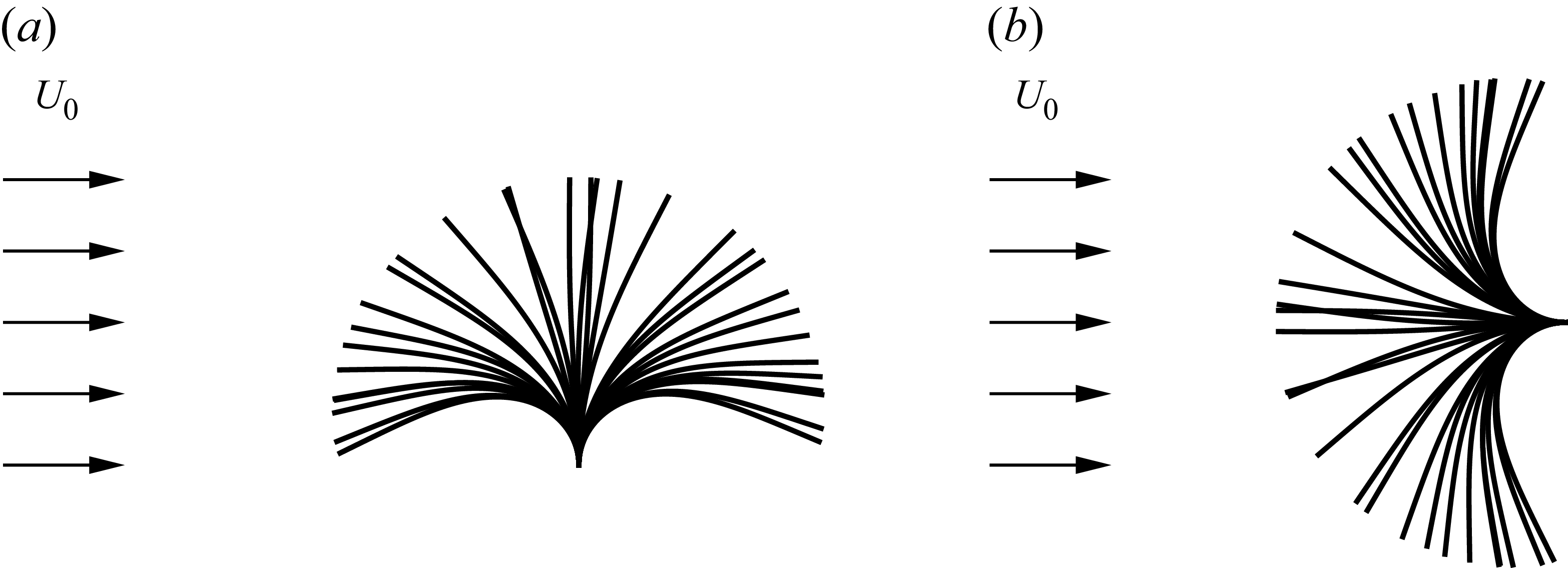
In the interaction of fluid flow with flexible structures, once the external fluid loading exceeds a critical value, the structure undergoes a deformation compliant to the flow and even loses its stability, leading to flow-induced vibration (Boukor et al. Reference Boukor, Choimet, Laurendeau and Gosselin2018). Reciprocally, the reconfigured or unsteady structural geometry in turn affects the fluid loading experienced by the structure (Alben et al. Reference Alben, Shelley and Zhang2002; Boukor et al. Reference Boukor, Choimet, Laurendeau and Gosselin2018), which creates a strong coupling between them. In the preceding section, we discussed the structure deformation and response, i.e. plate tip deflection, with varying critical parameters. Here, we examine the effect of the inclination angle on the hydrodynamic drag force acting on a thin flexible plate with varying bending stiffness in oscillatory flow.
Schematics of the profile superpositions of thin flexible plates in uniform incoming flow with inclination angle of (a)
 $90^{\circ }$
and (b)
 $0^{\circ }$
.

In figure 12, we present schematics of two extreme cases of thin flexible plates entering flapping regime under a uniform incoming flow with inclination angles of
 $0^{\circ }$
and
 $90^{\circ }$
. For the
 $90^\circ$
case, the thin flexible plate is placed vertically in a cross-flow, and the flow-induced reconfiguration reduces its frontal area and drag force (Luhar & Nepf Reference Luhar and Nepf2011). By contrast, when the thin flexible plate with zero inclination angle is positioned in the flow, theoretically, the form drag by pressure is negligible, while the skin friction drag plays a more important role. However, owing to the large-amplitude flapping of the thin flexible plate (see figure 12
b), it receives considerable pressure-induced drag force (Kim et al. Reference Kim, Cossé, Ceideira and Gharib2013). Therefore, these two extreme cases suggest that the inclination angle plays a crucial role in determining the drag force characteristics of the flexible plate, which is simultaneously dependent on the structure response behaviours governed by the competition between bending stiffness and fluid loading.
The ratio of the dimensionless root-mean-square (r.m.s.) drag force of the inclined flexible plate to that of rigid one,
 $\widetilde {C_d} / \widetilde {C_{d,0}}$
as a function of
 $CaL$
with varying
 ${\textit{KC}}$
at (a)
 $\alpha = 5^{\circ }$
, (b)
 $\alpha = 30^{\circ }$
, (c)
 $\alpha = 60^{\circ }$
and (d)
 $\alpha = 90^{\circ }$
. The solid lines represent the scaling laws in (4.34). The dimensionless arithmetic mean drag force,
 $\overline {C_d}$
,is shown in the corresponding insets.

To examine the influence of the bending stiffness and the inclination angle, in figure 13, we present the ratio of the dimensionless r.m.s. drag force of an inclined flexible plate to that of the corresponding rigid plate with varying
 $K_{\!B}$
number and Keulegan–Carpenter number for inclination angles
 $\alpha = 5^{\circ }$
,
 $30^{\circ }$
,
 $60^{\circ }$
and
 $90^{\circ }$
. In addition, the dimensionless arithmetic mean drag forces are shown in the inset figures. The r.m.s. drag forces of both flexible and rigid plates are calculated using the following equations:
 \begin{equation} \widetilde {F_d} = \sqrt {\frac {1}{T} \int _{0}^{T} F^2_d (t) \textrm {d} t}, \quad \textrm {and} \quad \widetilde {F_{d,0}} = \sqrt {\frac {1}{T} \int _{0}^{T} F^2_{d,0} (t) \textrm {d} t}, \end{equation}
where
 $F_d(t)$
and
 $F_{d,0}(t)$
denote the instantaneous drag force functions of the flexible and rigid plates, respectively, and
 $T$
is the period of the oscillatory flow. Accordingly, the ratio of the dimensionless r.m.s. drag force of the flexible plate to that of the rigid plate can be written as
 \begin{equation} \frac {\widetilde {C_d}}{\widetilde {C_{d,0}}} = \frac {\sqrt {\frac {1}{T} \int _{0}^{T} F^2_d (t) \textrm {d} t} / (\rho _{\!f} U_0^2 l)}{\sqrt {\frac {1}{T} \int _{0}^{T} F^2_{d,0} (t) \textrm {d} t} / (\rho _{\!f} U_0^2 l)} = \frac {\widetilde {F_d}}{\widetilde {F_{d,0}}}, \end{equation}
where
 $\widetilde {C_d}$
and
 $\widetilde {C_{d,0}}$
are the dimensionless r.m.s. drag forces. Meanwhile, the dimensionless arithmetic mean drag force,
 $\overline {C_d}$
, is calculated and normalised as
 \begin{equation} \overline {C_d} = \frac {1}{T} \int _{0}^{T} \frac {F_d(t)}{\rho _{\!f} U_0^2 l} \textrm {d} t. \end{equation}
In both mean drag force definitions, the mean values are averaged over 16 oscillation periods after the plate reaches the steady state for cases with regular responses, whereas for cases with irregular responses, the drag force is averaged over 40 periods.
In figure 13(a), it is observed that the flexible plate with a small inclination angle of
 $5^{\circ }$
exhibits drag forces essentially identical to those of a rigid plate over a wide range of
 ${\textit{CaL}}$
. Deviations occur only at very low stiffness, where irregular structural responses lead to increased drag force. On the other hand, for inclination angles
 $\alpha = 30^{\circ }$
,
 $60^{\circ }$
and
 $90^{\circ }$
in figure 13(b–d), the flexible plates exhibit closely similar trends in the variation of the drag ratio. When the combined parameter
 ${\textit{CaL}}$
is small (
 ${\textit{CaL}} \lt 1$
), indicating that fluid loading is significantly weak compared with the plate bending rigidity, the r.m.s. drag ratios are nearly independent of
 ${\textit{CaL}}$
and collapse onto the horizontal unity line. In this regime, the high structural bending stiffness forbids significant deflections, resulting in the plates experiencing the same drag force as the rigid ones. For some cases the drag ratio slightly exceeds unity, and similar behaviours are reported for a wall-mounted plate in oscillatory flow. This can be attributed to phase lag effects, which enhance the relative velocity between the plate and the oscillatory flow (Zhang & Nakamura Reference Zhang and Nakamura2024a
). From the perspective of vortex dynamics, for relatively stiff plates, a substantial fraction of the incoming flow kinetic energy is dissipated in the wake through strong shear layers (figure 8
a) and shed vortices (figure 9
a), resulting in high drag forces.
As the combined parameter
 ${\textit{CaL}}$
increases into the range of
 $O(1) - O(10)$
, a pronounced drag reduction is observed in figure 13(b–d), associated with increased structural reconfiguration. This enhanced reconfiguration arises from strengthened oscillatory flow (higher velocity and/or frequency) or reduced bending stiffness, both of which render the plate more deformable. Consequently, the effective projected area decreases due to reconfiguration, weakening the wake vortices and leading to a reduction in drag force. In this regime, the numerical results for the r.m.s. drag ratio collapse onto a straight line with a slope of
 $-1$
in a log–log representation. For larger values of
 ${\textit{CaL}}$
(
 ${\textit{CaL}} \gt 10$
), the r.m.s. drag ratio exhibits a slight but gradual increase followed by non-monotonic behaviour, which is attributed to the emergence of irregular flapping modes at very low bending stiffness.
To rationalise the observed trend of the r.m.s. drag force ratio for
 $\alpha = 30^{\circ }$
,
 $60^{\circ }$
and
 $90^{\circ }$
, we adopt the concept of the effective plate length introduced by Luhar & Nepf (Reference Luhar and Nepf2011) and Luhar & Nepf (Reference Luhar and Nepf2016). The effective plate length
 $l_e$
is defined as the length of a rigid plate that generates the same drag force as a flexible plate of total length
 $l$
, with both plates having the same inclination angle. This concept provides a convenient framework to quantify drag variations arising from frontal area reduction and streamlining effects induced by elastic reconfiguration. Under this formulation, the drag force can be evaluated using the same drag coefficient as that of a rigid plate. Accordingly, the ratio of r.m.s. drag forces can be expressed as
 \begin{equation} \frac {\widetilde {C_d}}{\widetilde {C_{d,0}}} = \frac {\widetilde {F_d}}{\widetilde {F_{d,0}}} = \frac {\widetilde {C_{d,0}} \rho _{\!f} U_0^2 l_e/2}{ \widetilde {C_{d,0}} \rho _{\!f} U_0^2 l/2} = \frac {l_e}{l} .\end{equation}
For small values of the combined parameter
 ${\textit{CaL}}$
(
 ${\textit{CaL}} \lt 1$
), the plate bending rigidity is sufficiently large that only negligible deflections occur under the oscillatory flow. The effective plate length therefore remains equal to the geometric length, i.e.
 $l_e / l = 1.0$
. As a result, the flexible and rigid plates experience essentially identical drag forces due to unaltered geometry features, and the r.m.s. drag ratio remains close to unity. On the other hand, in the parameter range where the reconfiguration-induced drag reduction becomes significant, the effective plate length variation can be elaborated by a scaling analysis of balance between the hydrodynamic fluid loading and the elastic restoring force of the structure. Under the external oscillatory flow, the flexible plate undergoes periodic flapping, back and forth, in one wave period, which gives rise to a tip deflection of the order of
 $O(a_w)$
, as shown in § 4.4. Similar to the derivation in § 4.4, the elastic restoring force of the flexible plate can be evaluated as
 \begin{equation} \textit{EI} \frac { {d}^2 \theta }{\textrm {d} s^2} \approx \textit{EI} \frac {a_w}{l^3}, \end{equation}
considering the geometry approximation
 $\theta \approx A/l \approx a_w/l$
. Following the definition of effective plate length, the balance between the hydrodynamic force exerted on the flexible plate and the elastic restoring force yields
 \begin{equation} \textit{EI} \frac {a_w}{l^3} \sim \frac {1}{2} C_d \rho _{\!f} U_0^2 l_e b \textrm {sin} \alpha + \frac {1}{2} C_l \rho _{\!f} U_0^2 l_e b \textrm {cos} \alpha \end{equation}
where
 $b$
is the width of the plate exposed to the impinging flow and treated as unity in our two-dimensional configuration, which further can be rewritten as
 \begin{equation} \frac {l_e}{l} \sim (\textit{CaL})^{-1}. \end{equation}
Indicated by (4.30), we can have the scaling results of r.m.s. drag force ratio as
 \begin{equation} \frac {\widetilde {C_d}}{\widetilde {C_{d,0}}} = \frac {l_e}{l} \sim (\textit{CaL})^{-1}, \end{equation}
of which the power of scaling law,
 $-1$
, agrees well with the numerical results in figure 13(b–d). The scaling results demonstrate that the observed drag reduction is primarily attributable to the decrease of effective plate length associated with the elastic reconfiguration of plates.
As shown in figure 13, it is also observed that the dimensionless arithmetic mean drag forces are generally close to zero, indicating that the instantaneous drag forces during the leftward and rightward strokes of the oscillatory flow are nearly symmetric. However, for moderate inclination angles (e.g.
 $\alpha = 30^{\circ }$
and
 $60^{\circ }$
),
 $\overline {C_d}$
exhibits distinct positive peaks when
 ${\textit{CaL}} \sim O(1)$
. These peaks collapse well when they are scaled by the combined parameter
 ${\textit{CaL}}$
. A non-zero mean drag implies a net momentum input to the plate, which can be attributed to a shift in the equilibrium position about which the plate flaps. Specifically, under these conditions, the mean deflected configuration slightly deviates from the initial undeformed position, leading to a weak asymmetry in the force response over a wave cycle.
4.7. Energy conversion
A strong fluid–structure interaction is established between the thin flexible plate and the oscillatory flow. The hydrodynamic forces exerted on the plate surface alter the geometric configuration and may even affect its stability, which further changes fluid loading reciprocally. Through this coupled process, the ambient flow performs mechanical work on the reconfigured and flapping plate.
Dimensionless averaged plate elastic strain energy as a function of
 ${\textit{CaL}}$
with varying
 ${\textit{KC}}$
number at (a)
 $\alpha = 5^{\circ }$
, (b)
 $\alpha = 30^{\circ }$
, (c)
 $\alpha = 60^{\circ }$
and (d)
 $\alpha = 90^{\circ }$
. The dash–dotted lines represent the zero value.

From an energetic perspective, this interaction can be interpreted as an energy transfer process. The work done by the fluid is converted into the kinetic energy of structural motion and the elastic strain energy associated with plate bending deformation. Subsequently, the elastic strain energy can be released into the kinetic energy of the vibrating plate, the vortex energy of shedding vortices and the viscous dissipation in the surrounding fluid. Overall, the energy transfer pathway proceeds from the kinetic energy of the oscillatory flow to the mechanical energy of the flapping plate.
In the context of harvesting renewable energy from environmental flows such as wind, water currents and waves, the elastic strain energy may be further converted into electrical energy using the techniques of piezoelectric materials (Orrego et al. Reference Orrego, Shoele, Ruas, Doran, Caggiano, Mittal and Kang2017; Hamlehdar, Kasaeian & Safaei Reference Hamlehdar, Kasaeian and Safaei2019) or triboelectric nanogenerator (Phan et al. Reference Phan, Shin, Jeon, Kang, Han, Kim, Kim, Kim, Hwang and Hong2017; Zhang et al. Reference Zhang, Meng, Xia, Deng, Dai, Hagedorn, Peng and Wang2020a ), enabling potential utilisations, such as providing power to small-scale offshore devices.
To explore the maximal potential of electricity power generation, we evaluate the elastic strain energy created by the structural deformation from the kinetic energy of the oscillatory flow, which is the foundation for electric energy utilisation. The evaluation is conducted by calculating the period-averaged elastic strain energy using the following expression:
 \begin{equation} E_s = \frac {1}{nT} \int _{t}^{t+nT} \int _{0}^{l} \frac {1}{2} EI \kappa ^2 \textrm {d}s\textrm {d}t, \end{equation}
where
 $\kappa$
is the local structural curvature,
 $EI$
is the bending stiffness and
 $T$
is the period of the oscillatory flow. The localised elastic strain energy is integrated along the plate and over multiple oscillatory periods. The period-averaged elastic strain energy is normalised by dynamic pressure
 $\rho _{\!f} U_0^2 l^2$
and denoted as
 $\overline {E_s}$
. Figure 14 presents the dimensionless period-averaged elastic strain energy
 $\overline {E_s}$
as a function of the combined parameter
 ${\textit{CaL}}$
for varying
 ${\textit{KC}}$
number at inclination angles
 $\alpha = 5^{\circ }$
,
 $30^{\circ }$
,
 $60^{\circ }$
and
 $90^{\circ }$
.
From figure 14, it is clearly observed that, for all inclination angles and Keulegan–Carpenter numbers, the dimensionless period-averaged elastic strain energy increase rapidly from zero value at very small
 ${\textit{CaL}}$
value until reaching a maximum value. Thereafter,
 $\overline {E_s}$
shows a swift decrease followed by the non-monotonic variation in the high
 ${\textit{CaL}}$
regime. At extremely low
 ${\textit{CaL}}$
, the plate remains nearly rigid and most of the fluid energy is dissipated in the wake, as shown in figures 8(a) and 9(a). The following increment of
 $\overline {E_s}$
can be explained by the fact that, at a fixed Keulegan–Carpenter number and inclination angle
 $\alpha$
, a decrease in
 $K_{\!B}$
, which by definition corresponds to an increase in
 ${\textit{CaL}}$
, renders the flexible plate less resistant to fluid loading. This promotes flapping with larger amplitudes and increased bending curvature. The combined effect of reduced bending stiffness and enhanced curvature gives rise to a continued growth of elastic strain energy. This is because the bending curvature
 $\kappa$
, which can be approximated as
 $\kappa \approx A/l^2$
as discussed in § 4.4, increases as the bending stiffness decreases in the fully reconfigured state. Moreover, the contribution of curvature growth dominates the effect of decreasing bending stiffness, since the elastic strain energy scales linearly with stiffness but quadratically with curvature, as indicated by (4.35). However, once the bending stiffness is sufficiently small for the plate to enter the passive movement state, the marginal contribution of curvature diminishes because the tip deflection saturates at the wave orbital excursion. Consequently, with nearly constant curvature and decreasing bending stiffness, the dimensionless elastic strain energy decreases. This rise-and-fall behaviour results in an optimal value of
 $\overline {E_s}$
, as shown in figure 14.
Around the optimal value, for example in the case shown in figure 9(b), the shed vortices are maintained in the vicinity of the plate leading edges, where they interact constructively with the plate, thereby promoting higher energy conversion. For lower bending stiffness, the plate becomes overly compliant to resist the shear imposed by the flow. Therefore, less fluid kinetic energy is transferred into the structural elastic strain energy, which is corroborated by the greatly weakened leading edge vortices observed in figure 9(c,d).
To further quantitatively elucidate the dependence of elastic strain energy on key parameters, namely the structural bending stiffness
 $K_{\!B}$
, the Keulegan–Carpenter number, and the inclination angle
 $\alpha$
, here we establish a scaling law model to show the influence of each aspect when the plate is in the fully reconfigured state. Based on the geometry of the deformed plate during bending, the radius of curvature can be approximated as
 \begin{equation} \frac {l}{R} = \theta \approx \frac {A}{l}, \end{equation}
which gives rise to a curvature as
 \begin{equation} \kappa = \frac {1}{R} \approx \frac {A}{l^2}. \end{equation}
According to the definitive expression of elastic strain energy of (4.35), the dimensionless elastic strain energy
 $\overline {E_s}$
scales as
 \begin{equation} \overline {E_s} \sim \frac {1}{T} \frac {EI}{\rho _{\!f} U_0^2 l^3} \frac {A^2}{l^4} l^2 T = \frac {EI}{\rho _{\!f} U_0^2 l^3} \frac {A^2}{a_w^2} \frac {a_w^2}{l^2}. \end{equation}
By substituting the definitions of dimensionless bending stiffness
 $K_{\!B} = EI/\rho _{\!f} U_0^2 l^3$
and length ratio
 $L = l/a_w$
, and applying the scaling law of tip deflection of plates in the fully reconfigured state,
 $A/a_w \sim CaL$
(4.20), we obtain the following scaling relation for
 $\overline {E_s}$
:
 \begin{equation} \overline {E_s} \sim {\textit{Ca}}^2K_{\!B}. \end{equation}
(a) Dimensionless plate elastic strain energy as a function of
 ${\textit{CaL}}$
with varying Keulegan–Carpenter number and multiple inclination angles coloured as shown in the colour bar. The solid lines represent the scaling laws in (4.39). (b) Optimal Cauchy number
 ${\textit{Ca}}_{\textit{opt}}$
at which the flexible plate achieves the highest elastic strain energy from the oscillatory flow of various
 ${\textit{KC}}$
number under inclination angles of
 $\alpha = 30^{\circ }$
,
 $60^{\circ }$
and
 $90^{\circ }$
. The solid lines represent the scaling laws in (4.42).

In figure 15(a), we plot the dimensionless averaged elastic strain energy as a function of combined parameter
 ${\textit{Ca}}^2K_{\!B}$
for varying structural bending stiffness, Keulegan–Carpenter number and plate inclination angle. The proposed scaling law (4.39) is in good agreement with the simulation results in the fully reconfigured state. Although some data points exhibit deviations towards higher values, these discrepancies can be attributed to resonance-induced large amplitude flapping, which leads to a reduced radius of curvature and, consequently, enhanced elastic strain energy.
After the growing elastic strain energy reaches its maximum peak,
 $E_s$
decreases beyond a turning point. As shown in figure 15(a), the locations of these turning points, corresponding to the maximal elastic strain energy, vary with plate inclination angle under different oscillatory flow conditions. To identify the critical condition for optimal elastic strain energy, namely the maximum energy-harvesting potential, we hypothesise that this optimum occurs at the transition between the fully reconfigured state and the passive movement state, as suggested by the observations and discussions above.
Since
 $E_s$
increases quadratically with the plate tip deflection
 $A$
, larger deflections are particularly favourable for enhancing
 $E_s$
, despite its linear dependence on the bending stiffness
 $K_{\!B}$
. The state transition of a flexible plate in oscillatory flow occurs when the plate is able to reach the fully reconfigured state under the averaged flow velocity within one stroke prior to flow reversal. Two characteristic time scales for the reconfiguration procedures are therefore introduced: the time scale of oscillatory flow,
 $T_w = 1/f_w$
, and the time scale of flexible plate reconfiguration in a unidirectional uniform flow with an averaged velocity,
 $T_{\textit{uni}} \sim A /U_{aver}$
, where
 $A$
denotes the mean horizontal deflection of plate tip and
 $U_{aver}$
is the averaged velocity of uniform flow. For a sinusoidal oscillatory flow, the averaged wave velocity is represented by its r.m.s. value,
 $U_0/\sqrt {2}$
. Achieving full reconfiguration before the oscillatory flow reversal requires that the time when the flexible plate reaches the fully reconfigured shape be shorter than half of the oscillatory flow period, which leads to
 \begin{equation} T_{\textit{uni}} \lt T_{w}/2. \end{equation}
Therefore, the critical condition for optimal elastic strain energy is obtained by setting the above inequality to equality, as
 \begin{equation} T_{\textit{uni}} = T_{w}/2, \end{equation}
where
 $T_{\textit{uni}} = \sqrt {2} A/U_0$
and
 $T_w = 1/f_w$
. Previous studies on flexible plates subjected to a unidirectional uniform flow have shown that the tip deflection follows the scaling law
 $A/l \sim Ca$
(Jerome et al. Reference Jerome, Bachelier, Doppler, Lehmann and Riviere2023; Kumar et al. Reference Kumar, Assam and Prabhakaran2023). Therefore, (4.41) can be derived into the following equation:
 \begin{equation} {\textit{Ca}}_{\textit{opt}} \sim KC. \end{equation}
The critical Cauchy number
 ${\textit{Ca}}_{\textit{opt}}$
for the optimal energy conversion of elastic strain energy characterises the ability of a flexible plate to convert the work done by fluid loading into elastic strain energy. Figure 15(b) shows the optimal Cauchy number of inclined flexible plates with different inclination angles
 $\alpha$
under oscillatory flows with varying Keulegan–Carpenter number
 ${\textit{KC}}$
, where the data points corresponding to the maximal elastic strain energy are extracted from the simulation results in figure 14. The scaling law prediction derived from the time scale shows good agreement with the numerical results that all optimal Cauchy numbers of different inclination angles and wave orbital excursions collapse on a solid line. This collapse further confirms that the modified Cauchy number successfully captures the influence of inclination angle on the dynamics of inclined flexible plates in oscillatory flows.
5. Conclusions
In the present study, we numerically investigate the dynamics of a two-dimensional inclined thin flexible plate subjected to a sinusoidally oscillating flow. The effects of bending stiffness, wave orbital excursion and inclination angle are examined, with particular emphasis on plate deflection, drag reduction and energy conversion relevant to potential renewable energy harvesting. An immersed boundary method is employed to model the fluid–structure interaction of thin flexible plate, in which a Navier–Stokes fluid solver is partitioned-coupled with a solid solver for the nonlinear Euler–Bernoulli beam model. The main findings of this study are summarised below.
Through systematic numerical simulations, we sweep the key governing parameters, including the dimensionless bending stiffness
 $K_{\!B}$
(the ratio of structural elastic restoring force to the hydrodynamic force), the Keulegan–Carpenter number (characterising the relative importance of unsteady and convective effects in the flow) and the inclination angles
 $\alpha$
. Four distinct structural response modes are identified, namely, the static mode, flapping mode, subharmonic flapping mode and irregular mode, based on the tip deflection angle histories and their power spectra. The critical condition,
 $K_{\textit{Bcri}}$
, for the transition from the static mode to the flapping mode is determined. To quantitatively elucidate the effect of inclination on the plate dynamics, we derive the expression of the lift force coefficient of an inclined rigid plate placed in the oscillatory flow analytically. By incorporating the newly derived lift force coefficient, we propose a modified Cauchy number that accounts for inclination effects from both geometric and mechanical perspectives. Specifically, the geometric effect is represented by the projected area in the flow direction, while the mechanical effect is captured through the inclination angle-dependent drag and lift force coefficients of an inclined rigid plate in oscillatory flow.
Based on the observed variation of tip deflection with respect to the governing parameters, the kinematic behaviours of the inclined thin flexible plate in oscillatory flow can be classified into two distinct states: a fully reconfigured state, in which a balance is achieved between the structural elastic restoring force and the hydrodynamics-driven force, and a passive movement state, in which the flexible plate is sufficiently compliant to follow the flow passively and its motion is constrained by the wave orbital excursion. In the fully reconfigured state, the amplitude of the tip deflection is well predicted by the proposed scaling law based on the modified Cauchy number,
 $A/a_w \sim CaL$
. In contrast, in the passive movement state, the tip deflection exhibits saturation and remains of order unity,
 $A/a_w \sim O(1)$
. At low values of the combined parameter
 ${\textit{CaL}}$
, the inclined flexible plate exhibits drag forces identical to those of the corresponding rigid plate, owing to negligible plate deflection. As
 ${\textit{CaL}}$
increases, the r.m.s. drag force ratio undergoes a pronounced drag reduction induced by the elastic reconfiguration of plates, following a
 $-1$
scaling law with
 ${\textit{CaL}}$
, i.e.
 $\widetilde {C_d} / \widetilde {C_{d,0}} \sim (\textit{CaL})^{-1}$
. This scaling behaviour can be rationalised using the effective plate length model. The energy conversion of fluid kinetic energy to structural elastic strain energy initially increases and subsequently decreases with increasing
 ${\textit{CaL}}$
, resulting in a maximal elastic strain energy for optimal energy conversion. We proposed the scaling law to describe the growth of the period-averaged elastic strain energy with decreasing bending stiffness in the fully reconfigured state,
 $\overline {E_s} \sim {\textit{Ca}}^2K_{\!B}$
. It is found that the optimal energy conversion occurs at the transition between the fully reconfigured state and the passive movement state. The critical condition follows the scaling
 ${\textit{Ca}}_{\textit{opt}} \sim KC$
, and the good agreement with simulation results further demonstrates that the modified Cauchy number successfully captures the inclination effect. In addition, the associated vortex dynamics of the flexible plate are analysed and discussed.
In the present study, only the flexible plate in a two-dimensional configuration is under investigation. The three-dimensional effect from the finite aspect ratio and lateral edge vortices can critically influence the plate dynamics and instability mechanisms. Additionally, a coupled fluid–structure-electric interaction model with an output electrical circuit can be utilised to assess the electrical energy generation from piezoelectric patch-based energy harvesting. These are beyond the scope of the present study and will be the focus of our future research.
Supplementary movies
Supplementary movies are available at https://doi.org/10.1017/jfm.2026.11379.
Acknowledgements
J.Z. acknowledges the support of Japanese Government (Monbukagakusho:MEXT) Scholarships from the Ministry of Education, Culture, Sports, Science and Technology of Japan.
Declaration of interests
The authors report no conflict of interest.