1 Introduction
Turbulence has been subject of research for more than a century. In that time significant advances had been made in the understanding of turbulent flows. Nevertheless, many developed and applied turbulence models still need to be tuned for specific problems to work accurately. This holds for turbulence models to close the Reynolds averaged Navier–Stokes equations (Spalart Reference Spalart2015) and becomes obvious in rather complex geometry flows (Bode & Friedrichs Reference Bode and Friedrichs2014). But also the immense number of methods and models available for scale resolving methods shows that there is a lack of universality (Sagaut, Deck & Terracol Reference Sagaut, Deck and Terracol2013). The desire for universal turbulence models that do not need tuning for different flow geometries is obvious.
To further progress such model development, it is necessary to know about the character of turbulent structures, their evolution and how they are distributed in a turbulent flow. Lagrangian dynamics offers a possibility to do this. Lagrangian dynamics, in contrast to Eulerian dynamics, describes a flow in a reference frame that is fixed to a fluid particle instead of an inertial system fixed to the flow domain. This allows a different perspective on the flow and permits other ways of describing turbulence. Regarding turbulence as an ensemble of structures of different sizes there is need to describe the character of these structures as well as their dynamics.
The velocity gradient tensor contains a great amount of information about a flow and its dynamics. In their review about ‘critical-point’ concepts, Perry & Chong (Reference Perry and Chong1987) summarized how local flow patterns can be characterized by just regarding the velocity gradient tensor at the location of interest. For incompressible flows, the method extracts information about the flow pattern in the vicinity of a fluid particle by determining the state of the fluid particle in the
 $QR$
phase space, where the
 $QR$
space is spanned by the second and third invariants,
 $Q$
and
 $R$
, of the velocity gradient tensor. From the point of view of a fluid particle located on a structure, it allows the distinction between four different states of the structure at the location of the particle. For this distinction the discriminant of the velocity gradient tensor
 $\unicode[STIX]{x1D6E5}$
takes an important role. For positive values of
 $\unicode[STIX]{x1D6E5}$
the velocity gradient tensor has one purely real eigenvalue and a complex conjugate pair of complex eigenvalues and therefore the fluid particle sits on a part of a structure that has a rotational character. If
 $\unicode[STIX]{x1D6E5}\leqslant 0$
, all eigenvalues of the velocity gradient tensor are purely real and the supporting structure is purely straining at the location of the fluid particle. Further, for negative values of the third invariant
 $R\leqslant 0$
we find two contracting directions and one stretching direction, whereas if
 $R$
is positive we find two stretching directions and one contraction direction of the structure at the location of the fluid particle. So four characteristic structure types can be described by vortical structures with stretching character
 $\unicode[STIX]{x1D6E5}>0$
;
 $R\leqslant 0$
(I); vortical structures with contracting character
 $\unicode[STIX]{x1D6E5}>0$
;
 $R>0$
(II); pure straining structures with flattening character
 $\unicode[STIX]{x1D6E5}\leqslant 0$
;
 $R>0$
(III); and pure straining structures with elongating character
 $\unicode[STIX]{x1D6E5}\leqslant 0$
;
 $R\leqslant 0$
(IV). Sketches of these topologies that can be determined from the values of
 $Q$
and
 $R$
can be found in Ooi et al. (Reference Ooi, Martin, Soria and Chong1999). More detailed explanations of the structure types can be found in Perry & Chong (Reference Perry and Chong1987), Meneveau (Reference Meneveau2011), Bechlars (Reference Bechlars2015). The interpretation of these structures has to be conducted with care however. The analysis description of the character of a structure is purely local, therefore it does not necessarily describe the actual shape of the structure in the flow field. In other words, the characteristic analysis describes the tendency of the development of a structure at a given point in space and time. However, in the current study we show that the local approach using advanced analysis provides sufficient information about the character of the development of a given structure.
The joint probability density function (joint p.d.f.) of
 $Q$
and
 $R$
(known as the
 $QR$
plot) describes the characteristic composition of turbulence in the flow. Due to the similar shape that the isolines of this joint p.d.f. develops for many flows, the
 $QR$
plot is often called teardrop (Soria et al.
Reference Soria, Sondergaard, Cantwell, Chong and Perry1994; Chong et al.
Reference Chong, Soria, Perry, Chacin, Cantwell and Na1998; Ooi et al.
Reference Ooi, Martin, Soria and Chong1999; Ganapathisubramani, Lakshminarasimhan & Clemens Reference Ganapathisubramani, Lakshminarasimhan and Clemens2008; Elsinga & Marusic Reference Elsinga and Marusic2010). However, variations from this teardrop shape have been found, e.g. experimentally in the production region behind a grid (Laizet, Vassilicos & Cambon Reference Laizet, Vassilicos and Cambon2013; Gomes-Fernandes, Ganapathisubramani & Vassilicos Reference Gomes-Fernandes, Ganapathisubramani and Vassilicos2014) and numerically through direct numerical simulation (DNS) for a turbulent channel flow (Blackburn, Mansour & Cantwell Reference Blackburn, Mansour and Cantwell1996) and turbulent boundary layers (TBL) (Chacin, Cantwell & Kline Reference Chacin, Cantwell and Kline1996; Wang & Lu Reference Wang and Lu2012; Bechlars & Sandberg Reference Bechlars and Sandberg2017). In the wake in the direct vicinity of the grid it can be seen that the so-called Vieillefosse tail (Vieillefosse Reference Vieillefosse1982) is reduced in length and the
 $QR$
plot develops a nearly symmetric shape. From DNS data of wall-bounded flows it was found that the Vieillefosse tail decreases with decreased distance to the wall. With the change of this joint probability distribution, consequently, the characteristic composition of turbulence in these flows also varies. The shapes of the
 $QR$
plot at the outer layer locations of the boundary layer match the teardrop shape. However, in the buffer layer Blackburn et al. (Reference Blackburn, Mansour and Cantwell1996), Chong et al. (Reference Chong, Soria, Perry, Chacin, Cantwell and Na1998), Wang & Lu (Reference Wang and Lu2012), Bechlars & Sandberg (Reference Bechlars and Sandberg2017) found that the tail towards high values of
 $R$
and low values of
 $Q$
shrinks compared to the location further away from the wall. Furthermore, the teardrop shape formed by the isolines of the p.d.f. appears to be more tilted counter-clockwise. Between the buffer layer and the viscous sublayer (VLS) the teardrop transforms to a nearly oval shape and becomes even more tilted counter-clockwise. Wang & Lu (Reference Wang and Lu2012) reduced the complexity of the
 $QR$
plots by integrating the joint p.d.f. over the area of the respective characteristic types in the
 $QR$
space and have shown the wall-normal distribution of the characteristic structure types. Bechlars & Sandberg (Reference Bechlars and Sandberg2017) confirmed these results for a turbulent boundary layer at a free stream Mach number of 0.5. The generally smooth changes in the outer layers are contrasted by the strong changes in the near-wall region. Especially the contracting vortical structures (II) have a relatively strong near-wall peak.
From a modelling perspective it is important to understand the evolution of turbulent structures that results in these compositions of turbulence. The Lagrangian dynamics of
 $Q$
and
 $R$
describes this evolution from a fluid particle’s point of view. This dynamics can be conditioned on
 $Q$
and
 $R$
themselves which allows us to study them via their mean trajectories in the
 $QR$
space (see, e.g. Martin et al.
Reference Martin, Ooi, Chong and Soria1998). This mean dynamics can be multiplied by the joint probability density function (p.d.f.) of
 $Q$
and
 $R$
to obtain the probability current. Since the joint p.d.f. is a non-negative function both mean dynamics and probability current have the same trajectories. As in this work we focus on the physical mechanisms rather than on the probability flow, we will restrict ourselves to the discussion of the mean trajectories in the results and discussion chapters. Nevertheless, the probability current plays an important role in terms of validating data via the trajectories in
 $QR$
space. Lozano-Durán, Holzner & Jiménez (Reference Lozano-Durán, Holzner and Jiménez2015) have shown that for incompressible, statistically stationary turbulence that is spatially homogeneous or integrated over a periodic domain, the probability current has to be divergence free and, hence, its trajectories in
 $QR$
space must be closed. How certain variation of this can be interpreted is found in their work. In cases that do not fulfil these criteria (as is the case for compressible, external, growing boundary layers), we have to rely on conventional methods to validate the accuracy of our data.
By neglecting viscosity and by considering only part of the pressure effect the restricted Euler system for the two invariants describes the effect of the nonlinear terms of the Navier–Stokes equations (Vieillefosse Reference Vieillefosse1982, Reference Vieillefosse1984). The solution for this system is invariant in the
 $QR$
space for incompressible flows. The influence of the pressure-Hessian tensor on the overall evolution has been investigated by Chevillard et al. (Reference Chevillard, Meneveau, Biferale and Toschi2008), Luethi, Holzner & Tsinober (Reference Luethi, Holzner and Tsinober2009), Suman & Girimaji (Reference Suman and Girimaji2013), Wilczek & Meneveau (Reference Wilczek and Meneveau2014), Lawson & Dawson (Reference Lawson and Dawson2015). Further, Jeong & Girimaji (Reference Jeong and Girimaji2003), Wilczek & Meneveau (Reference Wilczek and Meneveau2014), Lawson & Dawson (Reference Lawson and Dawson2015) analysed the effect of viscous diffusion on the dynamics of
 $Q$
and
 $R$
. The mean overall Lagrangian dynamics of the invariants has been studied using DNS data of homogeneous isotropic turbulence (HIT) (Martin et al.
Reference Martin, Ooi, Chong and Soria1998; Luethi et al.
Reference Luethi, Holzner and Tsinober2009; Wilczek & Meneveau Reference Wilczek and Meneveau2014) and particle image velocimetry (PIV) data of the outer layer of an experimental turbulent boundary layer (Elsinga & Marusic Reference Elsinga and Marusic2010; Lawson & Dawson Reference Lawson and Dawson2015). Luethi et al. (Reference Luethi, Holzner and Tsinober2009) further quantified the variance of the mean evolution and the coupling of the evolution with strain and rotation production. In a review Meneveau (Reference Meneveau2011) summarized most of the research done in the field of Lagrangian dynamics of the velocity gradient tensor. Models proposed by Chevillard et al. (Reference Chevillard, Meneveau, Biferale and Toschi2008) and Elsinga & Marusic (Reference Elsinga and Marusic2010) mimic the general characteristics of the
 $QR$
dynamics, but are not satisfactorily agreeing with experimental or numerical results. With the work of Chevillard et al. (Reference Chevillard, Meneveau, Biferale and Toschi2008) it became clear that the crucial part of an accurate model will be to capture the non-local effects of the pressure-Hessian tensor. Wilczek & Meneveau (Reference Wilczek and Meneveau2014) developed a stochastic model based on the assumption that the flow field fulfils the characteristics of Gaussian random fields. Through this they obtained a local closure for the viscous diffusion and the pressure Hessian. The coefficients for this model provided by the Gaussian random fields do lead to a diverging model. However, an adjustment of these coefficients based on DNS data improves the model. Although the work of Wilczek & Meneveau (Reference Wilczek and Meneveau2014) gives a deep and novel insight into the dynamics of the velocity gradient tensor, the link to turbulent structures in physical space remains open. This gap was closed by Lawson & Dawson (Reference Lawson and Dawson2015) who utilized stochastic estimations to obtain a closure for the viscous diffusion and the pressure-Hessian terms in the velocity gradient tensor dynamics. Their results, obtained through experiments, agree well with the DNS results of the enhanced Gaussian closure of Wilczek & Meneveau (Reference Wilczek and Meneveau2014). Further, they provide the structure of the averaged flow field conditioned on different characteristic states in the
 $QR$
space. Although this resembles only the superposition of many instantaneous events and not the actual instantaneous constellation, as pointed out by the authors, it still allows for an interesting impression of how the flow causes the different characteristic states reflected in the
 $QR$
space. Such insights are particularly helpful for understanding the non-local effects within the turbulence dynamics. In general, many approaches to model the velocity gradient dynamics have been proposed and it turns out that the non-local effects of the pressure-Hessian term are the most difficult to capture. Further, the most accurate models have been derived with HIT data, hence possible changes of the effect of the pressure Hessian due to inhomogeneities in the flow could not been examined.
Whereas the strain rate tensor governs the dissipation of kinetic energy, the coupling of both strain rate tensor and rotation rate tensor governs the process of vortex stretching and vortex compression (Tsinober Reference Tsinober2000; Hamlington, Schumacher & Dahm Reference Hamlington, Schumacher and Dahm2008). In the above discussed dynamics of turbulence, this vortex dynamics is considered as a key quantity as it drives the turbulent cascading process. Luethi et al. (Reference Luethi, Holzner and Tsinober2009) studied the production of strain and rotation as a function of the second invariant
 $Q$
of the velocity gradient tensor using HIT data obtained through DNS. They found that the fluid particles successively encounter high enstrophy/strain production events, enstrophy dominated regions, vortex compression events and strain dominated regions along the mean trajectories in
 $QR$
space. They concluded that the non-locality plays a crucial role for the evolution of the velocity gradients.
All of the analyses of the dynamics have been conducted analytically or in flow regions where a distinct teardrop shape of the
 $QR$
plot has developed. The varying
 $QR$
plots in cases such as a TBL are certainly caused by a change of the underlying dynamics. This variation of the dynamics has so far not been investigated. In this work we study the mean evolution of turbulent structures as represented in the
 $QR$
space. Of particular interest is the variation of the evolution for different wall-normal locations in a TBL and determining how this causes the different characteristic distribution of turbulence represented by the varying joint p.d.f. of
 $Q$
and
 $R$
. The DNS that was carried out to provide the compressible dataset is outlined in § 2. In § 3 a novel compressible evolution system for the first three invariants of the velocity gradient tensor is derived. The results of this work are shown in § 4. The resulting mean evolution at different locations in the TBL is shown in § 4.1 and the contribution of its separate terms is shown in § 4.2. In § 5 these results are discussed, put into context with other turbulent flows. Conclusions are drawn in § 6.
2 Flow data
A DNS of a compressible zero pressure gradient turbulent boundary layer (TBL) (Bechlars & Sandberg Reference Bechlars and Sandberg2017) was carried out to investigate the features that will be outlined in the following. The coordinates
 $x,y$
and
 $z$
denote the streamwise, wall-normal and spanwise coordinates, respectively. Accordingly
 $u,v$
and
 $w$
denote the streamwise, wall-normal and spanwise velocity components;
 $\unicode[STIX]{x1D70C}$
is the density,
 $p$
the static pressure,
 $T$
the temperature and
 $\unicode[STIX]{x1D707}$
the dynamic viscosity. We consider a single phase compressible fluid being a continuum, fulfilling the Newtonian conditions and the properties of a perfect caloric gas. We introduce the notation
 $\bar{\bullet }$
for Reynolds averaged quantities/terms,
 $\tilde{\bullet }$
for density averaged Favre averaged quantities/terms and
 $\bullet ^{\prime \prime }$
denotes the fluctuations around Favre averaged quantities. Further, we introduce a wall scaling (which is marked by a superscript
 $+$
) based on the friction velocity
 $u_{\unicode[STIX]{x1D70F}}=\sqrt{(\unicode[STIX]{x1D707}_{wall}/\mathit{Re }_{\infty }\,\unicode[STIX]{x1D70C}_{wall})(\unicode[STIX]{x2202}\tilde{u} /\unicode[STIX]{x2202}y)}$
at the particular streamwise location. Thus
 $l^{+}=l(\mathit{Re}_{\infty }\,\unicode[STIX]{x1D70C}_{wall}u_{\unicode[STIX]{x1D70F}}/\unicode[STIX]{x1D707}_{wall})$
and
 $v^{+}=v/u_{\unicode[STIX]{x1D70F}}$
. Energies and velocity products
 $g$
are scaled as
 $g^{+}=g(1/u_{\unicode[STIX]{x1D70F}}^{2})$
and the terms
 $b$
of the energy budget are scaled with a density weighted scaling as
 $b^{+}=b(T/\mathit{Re}_{\infty }\,\unicode[STIX]{x1D70C}^{2}u_{\unicode[STIX]{x1D70F}}^{4})$
.
The Reynolds number range of the TBL is
 $\mathit{Re}_{\unicode[STIX]{x1D703}}\approx 670{-}2330$
(
 $\mathit{Re}_{\unicode[STIX]{x1D70F}}\approx 220{-}830$
) and therefore in the fully developed turbulent regime. The Mach number in the free stream is
 $M_{\infty }=0.5$
and the free stream Prandtl number
 $\mathit{Pr}_{\infty }=0.72$
. The wall is set to be isothermal at the adiabatic temperature of the free stream
 $T_{wall}\approx 1.05$
. In order to obtain a turbulent boundary layer an artificial turbulent inflow condition (Touber & Sandham Reference Touber and Sandham2009) was applied. The outflow is a characteristic outflow condition (Poinsot & Lele Reference Poinsot and Lele1992) to minimize artificial reflections. The free stream is an ordinary non-reflective characteristic boundary condition (Thompson Reference Thompson1990). A more detailed description of the methods used for the DNS can be found in Bechlars (Reference Bechlars2015).
The data are obtained from fully resolved direct numerical simulations with an in-house compressible Navier–Stokes solver (Sandberg Reference Sandberg2015). The spatial discretization is performed using fourth-order accurate standard differences in the streamwise and wall-normal directions, whereas the spanwise direction is discretized using the Fourier decomposition. For the discretization of time a fourth-order accurate five-step Runge–Kutta method was chosen. Further details of the numerical methods are outlined in Bechlars (Reference Bechlars2015), Sandberg (Reference Sandberg2015). The grid for the decomposition is a structured Cartesian mesh and counts
 $7200\times 260$
points in the streamwise and wall-normal directions, respectively. One hundred and ninety-three spanwise Fourier modes were used to discretize the spanwise direction. This leads to a total of approximately 723 million collocation points in the domain. The grid is stretched in the streamwise direction to keep the wall-scaled spacing relatively constant. The streamwise spacing has an upper bound of
 $\unicode[STIX]{x0394}x^{+}<5.12$
throughout the entire domain. The wall-normal location of the first point off the wall (
 $y=0$
) is located at
 $y^{+}|_{1}\approx 0.600{-}0.712$
and the tenth grid point is located at
 $y^{+}|_{10}\approx 5.43{-}6.40$
. The collocation points in the spanwise direction have a spacing of
 $\unicode[STIX]{x0394}z^{+}\approx 3.72{-}4.38$
.
The data for the following investigations were obtained in a volume that reaches from
 $\mathit{Re}_{\unicode[STIX]{x1D703}}\approx 1224{-}1248$
(
 $\mathit{Re}_{\unicode[STIX]{x1D70F}}\approx 481{-}491$
) in the streamwise direction, covers approximately 120 % of the local boundary layer thickness
 $\unicode[STIX]{x1D6FF}_{99}(\mathit{Re}_{\unicode[STIX]{x1D703}}=1230)$
and spans over the full spanwise extent of the domain. The sample volume is short enough that statistical homogeneity can be assumed over its streamwise extent, in addition to the spanwise direction. The statistics in the result chapters are sampled over a non-dimensional time period of
 $\unicode[STIX]{x0394}{\mathcal{T}}\approx 90.4((\unicode[STIX]{x1D6FF}_{99}(\mathit{Re}_{\unicode[STIX]{x1D703}}=1230))/U_{\infty })$
.
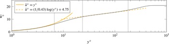
Profile of the streamwise mean velocity component over the distance to the wall in wall-scaling units at
 $\mathit{Re}_{\unicode[STIX]{x1D703}}\approx 1230$
. The continuous and dashed yellow lines indicate the linear behaviour in the viscous sublayer (VSL) and a logarithmic law for the development of the velocity, respectively. The vertical grey lines indicate locations at which data are plotted in the results section.

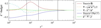
Profile of the turbulent kinetic energy budget over the distance to the wall in wall-scaling units at
 $\mathit{Re}_{\unicode[STIX]{x1D703}}\approx 1230$
. The vertical grey lines indicate locations at which data are plotted in the results chapter.

In figures 1 and 2 the vertical lines mark the wall-normal locations that are chosen for more detailed analysis in the results chapter. Overall it can be stated that the wall-normal gradient of the mean streamwise velocity component and other quantities vary strongly over the wall-normal distance. These gradients are the driving force of turbulence in this particular flow and the effect of their wall-normal variations are investigated in the next section.
3 Compressible velocity gradient tensor invariant dynamics
The dynamics of the velocity gradient tensor invariants is derived from the velocity gradient tensor dynamics. The dynamics for the velocity gradient tensor
 $\unicode[STIX]{x1D63C}:=\unicode[STIX]{x1D735}\boldsymbol{u}$
is obtained by subtracting the continuity equation multiplied by the velocity vector from the momentum equation. The result is divided by the density and finally the gradient is taken of the entire equation. This leads to
 $$\begin{eqnarray}\frac{\text{d}\unicode[STIX]{x1D63C}}{\text{d}t}:=\frac{\unicode[STIX]{x2202}\unicode[STIX]{x1D63C}}{\unicode[STIX]{x2202}t}+(\boldsymbol{u}\boldsymbol{\cdot }\unicode[STIX]{x1D735})\unicode[STIX]{x1D63C}=-\unicode[STIX]{x1D63C}\unicode[STIX]{x1D63C}+\unicode[STIX]{x1D643}.\end{eqnarray}$$
The source term
 $\unicode[STIX]{x1D643}$
 $$\begin{eqnarray}\unicode[STIX]{x1D643}:=\unicode[STIX]{x1D71E}-\unicode[STIX]{x1D72E}\end{eqnarray}$$
combines the viscous effects
 $\unicode[STIX]{x1D71E}$
acting on the velocity gradient
 $$\begin{eqnarray}\unicode[STIX]{x1D71E}=\unicode[STIX]{x1D735}\left(\frac{1}{\unicode[STIX]{x1D70C}}\unicode[STIX]{x1D735}\boldsymbol{\cdot }\unicode[STIX]{x1D749}\right),\end{eqnarray}$$
where
 $\unicode[STIX]{x1D749}$
denotes the viscous stress tensor, with the pressure–density term
 $\unicode[STIX]{x1D72E}$
 $$\begin{eqnarray}\unicode[STIX]{x1D72E}=\unicode[STIX]{x1D735}\left(\frac{1}{\unicode[STIX]{x1D70C}}\unicode[STIX]{x1D735}p\right).\end{eqnarray}$$
For the derivation of the velocity gradient invariants we need to introduce the dynamics of the second and third power of the velocity gradient tensor. The dynamics of the second power of the velocity gradient tensor is
 $$\begin{eqnarray}\frac{\text{d}\unicode[STIX]{x1D63C}^{2}}{\text{d}t}=-2\unicode[STIX]{x1D63C}^{3}+\unicode[STIX]{x1D63C}\unicode[STIX]{x1D643}+\unicode[STIX]{x1D643}\unicode[STIX]{x1D63C}.\end{eqnarray}$$
The dynamics of the third power of the velocity gradient tensor is
 $$\begin{eqnarray}\frac{\text{d}\unicode[STIX]{x1D63C}^{3}}{\text{d}t}=-3\unicode[STIX]{x1D63C}^{4}+\unicode[STIX]{x1D63C}^{2}\unicode[STIX]{x1D643}+\unicode[STIX]{x1D63C}\unicode[STIX]{x1D643}\unicode[STIX]{x1D63C}+\unicode[STIX]{x1D643}\unicode[STIX]{x1D63C}^{2}.\end{eqnarray}$$
Before deriving the compressible velocity gradient tensor invariant dynamics we need to introduce the invariants that we want to investigate. The first three invariants
 $P$
,
 $Q$
and
 $R$
of the
 $3\times 3$
matrix
 $\unicode[STIX]{x1D63C}$
are defined via the characteristic polynomial of the matrix
 $\unicode[STIX]{x1D63C}$
 $$\begin{eqnarray}p_{char}(\unicode[STIX]{x1D6FC}):=\det (\unicode[STIX]{x1D63C}-\unicode[STIX]{x1D6FC}\unicode[STIX]{x1D644})=\unicode[STIX]{x1D6FC}^{3}+P\unicode[STIX]{x1D6FC}^{2}+Q\unicode[STIX]{x1D6FC}+R,\end{eqnarray}$$
where
 $\unicode[STIX]{x1D644}$
is the identity matrix and can be calculated as
 $$\begin{eqnarray}\displaystyle & \displaystyle P=-\text{trace}(\unicode[STIX]{x1D63C})=-\unicode[STIX]{x1D735}\boldsymbol{\cdot }\boldsymbol{u}, & \displaystyle\end{eqnarray}$$
 $$\begin{eqnarray}\displaystyle & \displaystyle Q={\textstyle \frac{1}{2}}(\text{trace}(\unicode[STIX]{x1D63C})^{2}-\text{trace}(\unicode[STIX]{x1D63C}\unicode[STIX]{x1D63C}))={\textstyle \frac{1}{2}}(P^{2}-\text{trace}(\unicode[STIX]{x1D63C}^{2})), & \displaystyle\end{eqnarray}$$
 $$\begin{eqnarray}\displaystyle & \displaystyle R=-\text{det}(\unicode[STIX]{x1D63C})=-{\textstyle \frac{1}{3}}(P^{3}-3PQ+\text{trace}(\unicode[STIX]{x1D63C}^{3})). & \displaystyle\end{eqnarray}$$
Another invariant of the velocity gradient tensor that is used in this work is the discriminant of the characteristic polynomial (denoted as discriminant of the velocity gradient tensor in the following)
 $$\begin{eqnarray}\unicode[STIX]{x1D6E5}:=-{\textstyle \frac{1}{4}}P^{2}Q^{2}+Q^{3}+P^{3}R+{\textstyle \frac{27}{4}}R^{2}-{\textstyle \frac{18}{4}}PQR.\end{eqnarray}$$
With the definition of the first invariant of the velocity gradient tensor (3.8) we obtain its dynamics by taking the trace of the velocity gradient tensor dynamics (3.1) and multiplying it by
 $-1$
 $$\begin{eqnarray}\frac{\text{d}P}{\text{d}t}=P^{2}-2Q-\text{trace}(\unicode[STIX]{x1D643}).\end{eqnarray}$$
We can simplify the following expressions if we split the pressure and viscous stress matrix
 $\unicode[STIX]{x1D643}$
into a traceless part
 $\unicode[STIX]{x1D643}^{\ast }$
and a diagonal matrix containing the trace information
 $$\begin{eqnarray}\unicode[STIX]{x1D643}=\unicode[STIX]{x1D643}^{\ast }+{\textstyle \frac{1}{3}}\text{trace}(\unicode[STIX]{x1D643})\unicode[STIX]{x1D644}.\end{eqnarray}$$
This decomposition will be used for all terms that involve
 $\unicode[STIX]{x1D643}$
. The following identity will also be used to simplify the dynamics for the second invariant
 $$\begin{eqnarray}\text{trace}(\unicode[STIX]{x1D63C}\unicode[STIX]{x1D643})=\text{trace}(\unicode[STIX]{x1D63C}\unicode[STIX]{x1D643}^{\ast })+{\textstyle \frac{1}{3}}\text{trace}(\unicode[STIX]{x1D643})\text{trace}(\unicode[STIX]{x1D63C}).\end{eqnarray}$$
With the definition of the second invariant of the velocity gradient tensor (3.9) we obtain its dynamics by subtracting the trace of the second velocity gradient tensor dynamics (3.5) from the dynamics of
 $P$
(3.12) squared
 $$\begin{eqnarray}\frac{\text{d}Q}{\text{d}t}=QP-\frac{2}{3}P\,\text{trace}(\unicode[STIX]{x1D643})-3R-\text{trace}(\unicode[STIX]{x1D63C}\unicode[STIX]{x1D643}^{\ast }).\end{eqnarray}$$
For a simplified expression of the dynamics of the third invariant the decomposition (3.13) is applied to
 $\text{trace}(\unicode[STIX]{x1D63C}^{2}\unicode[STIX]{x1D643})$
. This results in
 $$\begin{eqnarray}\text{trace}(\unicode[STIX]{x1D63C}^{2}\unicode[STIX]{x1D643})=\text{trace}(\unicode[STIX]{x1D63C}^{2}\unicode[STIX]{x1D643}^{\ast })+{\textstyle \frac{1}{3}}\text{trace}(\unicode[STIX]{x1D643})\text{trace}(\unicode[STIX]{x1D63C}^{2}).\end{eqnarray}$$
Further, we will make use of the Cayley–Hamilton theorem which states that ‘Every square matrix satisfies its own characteristic equation’. It directly leads to the equation
 $$\begin{eqnarray}\unicode[STIX]{x1D63C}^{3}+P\unicode[STIX]{x1D63C}^{2}+Q\unicode[STIX]{x1D63C}+R\unicode[STIX]{x1D644}=0.\end{eqnarray}$$
Multiplying this equation with
 $\unicode[STIX]{x1D63C}$
and taking the trace of the product leads to the identity
 $$\begin{eqnarray}\text{trace}(\unicode[STIX]{x1D63C}^{4})=P^{4}-4P^{2}Q+2Q^{2}+4PR.\end{eqnarray}$$
With the definition of the third invariant of the velocity gradient tensor (3.10) we obtain its dynamics as
 $$\begin{eqnarray}\displaystyle & \displaystyle \frac{\text{d}R}{\text{d}t}=-{\textstyle \frac{1}{3}}Q\,\text{trace}(\unicode[STIX]{x1D643})+PR-P\,\text{trace}(\unicode[STIX]{x1D63C}\unicode[STIX]{x1D643}^{\ast })-\text{trace}(\unicode[STIX]{x1D63C}^{2}\unicode[STIX]{x1D643}^{\ast }). & \displaystyle\end{eqnarray}$$
A detailed step-by-step description of this brief summary of the novel derivation of the compressible dynamics for the first three invariants of the velocity gradient tensor can be found in Bechlars (Reference Bechlars2015). The system formed by these dynamics can be summarized as
 $$\begin{eqnarray}\displaystyle & \displaystyle \frac{\text{d}P}{\text{d}t}=P^{2}-2Q-\text{trace}(\unicode[STIX]{x1D643}), & \displaystyle\end{eqnarray}$$
 $$\begin{eqnarray}\displaystyle & \displaystyle \frac{\text{d}Q}{\text{d}t}=QP-\frac{2}{3}P\,\text{trace}(\unicode[STIX]{x1D643})-3R-\text{trace}(\unicode[STIX]{x1D63C}\unicode[STIX]{x1D643}^{\ast }), & \displaystyle\end{eqnarray}$$
 $$\begin{eqnarray}\displaystyle & \displaystyle \frac{\text{d}R}{\text{d}t}=-\frac{1}{3}Q\,\text{trace}(\unicode[STIX]{x1D643})+PR-P\,\text{trace}(\unicode[STIX]{x1D63C}\unicode[STIX]{x1D643}^{\ast })-\text{trace}(\unicode[STIX]{x1D63C}^{2}\unicode[STIX]{x1D643}^{\ast }). & \displaystyle\end{eqnarray}$$
 $\unicode[STIX]{x1D63C}$
and
 $\unicode[STIX]{x1D643}$
are not directly depending solely on
 $P,Q$
and
 $R$
. If one were to evolve these transport equations over time, additional closure terms derived from the Navier–Stokes equations would be required. However, in this work we use this system only to post-process and analyse datasets obtained by DNS. This means we have all separate terms available and exploit this novel system for the interpretation of our compressible results.
4 Results
The results are structured such that first the overall Lagrangian dynamics together with its consequences on strain and rotation production at different locations in the TBL are outlined. This is then followed by the contributions of the separate terms of the overall dynamics.
4.1
 $QR$
-phase flow as function of wall-normal location

The characteristic decomposition based on the critical-point concept (Perry & Chong Reference Perry and Chong1987) is purely local and describes the character of a structure at the location of the current fluid particle only. It does not describe the character of a structure as a whole. The method distinguishes between different characteristic local flow topologies depending on the first three velocity gradient invariants
 $P,Q$
and
 $R$
. These invariants span a state space, the
 $PQR$
-space, in which we find certain regions defining certain properties of the local flow topology at the fluid particle.
 $P$
, which is the additive inverse of the dilatation
 $-\unicode[STIX]{x1D735}\boldsymbol{\cdot }\boldsymbol{u}$
, is zero for incompressible flows. For compressible cases
 $P$
is not necessarily zero. However, for our results at a Mach number of
 $M_{\infty }=0.5$
we find no significant dependency of the results on
 $P$
. Therefore we map the results obtained from the compressible analysis onto the subset of the
 $PQR$
-space defined by
 $P=0$
, this we call
 $QR$
-space. The legitimacy for this step will be presented during the discussion of figure 5 in § 4.2. The distinction of characteristic topologies is made in analogy to the incompressible case as explained in Perry & Chong (Reference Perry and Chong1987) and Bechlars (Reference Bechlars2015) and summarized in the introduction.
For the following we introduce a scaling based on the local variance of the velocity gradient tensor magnitude
 $$\begin{eqnarray}\text{var}(\unicode[STIX]{x1D63C})=\overline{\text{trace}((\unicode[STIX]{x1D63C}-\bar{\unicode[STIX]{x1D63C}})(\unicode[STIX]{x1D63C}-\bar{\unicode[STIX]{x1D63C}})^{\text{T}})}.\end{eqnarray}$$
This is a measure for the variation of the velocity gradient tensor magnitude and it can be seen as a gradient analogue to the turbulent kinetic energy. The velocity gradient tensor quantities are scaled as
 $\hat{\unicode[STIX]{x1D63C}}=\unicode[STIX]{x1D63C}/\sqrt{\text{var}(\unicode[STIX]{x1D63C})}$
. According to this normalization the second and third invariants of the velocity gradient tensor are normalized using the variance of the velocity gradient tensor
 $\hat{Q}=Q/\text{var}(\unicode[STIX]{x1D63C})$
,
 $\hat{R}=R/\text{var}(\unicode[STIX]{x1D63C})^{3/2}$
. Time can be normalized as
 $\hat{t}=t\sqrt{\text{var}(\unicode[STIX]{x1D63C})}$
.
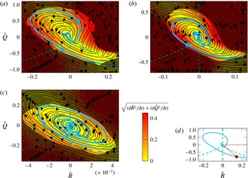
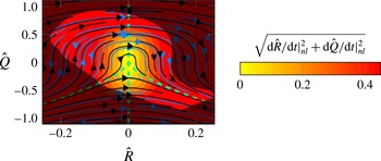
(a–c) The mean
 $QR$
-phase development of fluid particles at three different locations ((a)
 $y^{+}\approx 180$
, (b)
 $y^{+}\approx 24$
, (c)
 $y^{+}\approx 6.7$
) is shown by trajectories (black) and by the magnitude of the mean phase velocity (contours). The blue line indicates the trajectory used for the following analysis. The bright area covers 95 % of all events and the dashed green lines divide the
 $QR$
-phase space into the four characteristic local flow topology sectors. (d) Schematic explanation for the angle
 $\unicode[STIX]{x1D6FC}$
used in the following analysis.

To understand and interpret the changes of the
 $QR$
-plots in TBLs we study the evolution of turbulent structures in the
 $QR$
-phase space. The mean trajectories of the evolution derived in § 3 are shown in figure 3 for three different wall-normal locations. Instantaneously the dynamics shows strong deviations around these mean trajectories which results in significant standard deviations of the dynamics. Although not an exact description of the physics, the mean dynamics allows a valid basis to interpret the underlying physics.
The work of Lozano-Durán et al. (Reference Lozano-Durán, Holzner and Jiménez2015) revealed that integrating over a statistically inhomogeneous region can considerably bias the Lagrangian statistics. The reason for this becomes clear in the following as we see that the dynamics varies strongly in the inhomogeneous direction in the present TBL. A superposition of these results caused by integrating in the wall-normal direction would make it difficult to interpret the results. The mean dynamics data presented in this work were integrated in the homogeneous spanwise direction, about an extent of approximately 100 plus units in the streamwise direction and approximately 5 grid points in the wall-normal direction for each location. This results in
 $\unicode[STIX]{x0394}y^{+}\approx 3.34$
for the location at
 $y^{+}\approx 6.7$
,
 $\unicode[STIX]{x0394}y^{+}\approx 3.44$
for the location at
 $y^{+}\approx 24$
and
 $\unicode[STIX]{x0394}y^{+}\approx 21.1$
for the location at
 $y^{+}\approx 180$
. Therefore the turbulence within the integration area is regarded as quasi-statistically homogeneous.
For the outer most region at
 $y^{+}\approx 180$
we find similar trajectories to those reported for an HIT flow (Martin et al.
Reference Martin, Ooi, Chong and Soria1998) and the outer layer of an experimental TBL (Elsinga & Marusic Reference Elsinga and Marusic2010). However, the trajectories that we find for the outer layer of the present TBL are spiralling inwards faster than the ones for the TBL investigated experimentally. This is believed to have two reasons. One is that the present data were sampled at a lower Reynolds number than the data for the experimental results. The other reason is that due to the size of the interrogation windows used in the PIV, the data of Elsinga & Marusic (Reference Elsinga and Marusic2010) are missing part of the energy in the dissipation range of the spectrum, as also stated in their work. Both result in a weaker diffusion term whose role it is to drive the evolution towards the origin as we have highlighted in the introduction and as we will see later also holds for the present results. The weaker diffusion therefore leads to trajectories that are spiralling inwards less strongly.
The bright area in the plots (figure 3) cover 95 % of all events observed in the flow at the respective locations. Consequently, the darker areas represent 5 % of the events. These areas are darkened as we want to turn the attention to the main events in the flow.
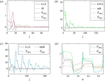
Development of the scaled invariants
 $\hat{\unicode[STIX]{x1D6E5}}$
and
 $\hat{R}$
as well as the scaled production of rotation
 $\hat{{\mathcal{P}}}_{\Vert \unicode[STIX]{x1D734}\Vert _{F}^{2}}=({\mathcal{P}}_{\Vert \unicode[STIX]{x1D734}\Vert _{F}^{2}}/\text{var}(\unicode[STIX]{x1D63C})^{3/2})$
and strain
 $\hat{{\mathcal{P}}}_{\Vert \unicode[STIX]{x1D64E}\Vert _{F}^{2}}=({\mathcal{P}}_{\Vert \unicode[STIX]{x1D64E}\Vert _{F}^{2}}/\text{var}(\unicode[STIX]{x1D63C})^{3/2})$
along the blue trajectories in figure 3. (a–c) Developments over scaled time
 $\hat{t}$
at
 $y^{+}\approx 180$
(a),
 $y^{+}\approx 24$
(b) and
 $y^{+}\approx 6.7$
(c). (d) Comparative development of the productions scaled with the velocity gradient tensor magnitude
 $\breve{{\mathcal{P}}}_{\Vert \unicode[STIX]{x1D64E}\Vert _{F}^{2}}=({\mathcal{P}}_{\Vert \unicode[STIX]{x1D64E}\Vert _{F}^{2}}/\overline{\text{trace}(\unicode[STIX]{x1D63C}\unicode[STIX]{x1D63C})})$
and
 $\breve{{\mathcal{P}}}_{\Vert \unicode[STIX]{x1D734}\Vert _{F}^{2}}=({\mathcal{P}}_{\Vert \unicode[STIX]{x1D734}\Vert _{F}^{2}}/\overline{\text{trace}(\unicode[STIX]{x1D63C}\unicode[STIX]{x1D63C})})$
at all locations over angle
 $\unicode[STIX]{x1D6FC}$
defined in figure 3. The colour scheme is taken from (a–c).

To obtain more insight into the processes taking place along the trajectories we pick one mean trajectory at each location (highlighted in blue in figure 3) and plot mean profiles conditioned with the respective
 $QR$
-state along these trajectories. Figure 4(a–c) shows the data over time for the trajectories at the respective wall-normal locations. For the development of the discriminant
 $\unicode[STIX]{x1D6E5}$
and the third invariant
 $R$
of the velocity gradient tensor we found the cycling periods in time normalized by the variance of the velocity gradient tensor to be approximately between
 $33\hat{t}-42\hat{t}$
for
 $y^{+}\approx 180$
, approximately between
 $34\hat{t}-52\hat{t}$
for
 $y^{+}\approx 24$
and approximately between
 $35\hat{t}-47\hat{t}$
for
 $y^{+}\approx 6.7$
. Time scaled with the eddy turnover time is defined as
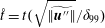 $\mathring{t}=t(\sqrt{\widetilde{\Vert \boldsymbol{u}^{\prime \prime }\Vert }}/\unicode[STIX]{x1D6FF}_{99})$
. Scaled with the eddy turnover time the cycling periods are
 $5.1\mathring{t}{-}6.4\mathring{t}$
,
 $2.5\mathring{t}{-}3.9\mathring{t}$
and
 $1.8\mathring{t}{-}2.5\mathring{t}$
, respectively. Except for the outermost cycle of the trajectory for the location closest to the wall, all cycling periods become larger the closer the
 $QR$
-state is to the origin of the
 $QR$
-phase space. Therefore the characteristic evolution process of turbulent structures in the
 $QR$
-phase space is slowed down the closer the structures come to the origin.
The processes occurring along the mean trajectories is explained in more detail by studying the production of rotation rate magnitude squared
 ${\mathcal{P}}_{\Vert \unicode[STIX]{x1D734}\Vert _{F}^{2}}=4\,\text{trace}(\unicode[STIX]{x1D734}\unicode[STIX]{x1D734}\unicode[STIX]{x1D64E})$
and strain rate magnitude squared
 ${\mathcal{P}}_{\Vert \unicode[STIX]{x1D64E}\Vert _{F}^{2}}=-2\,\text{trace}(\unicode[STIX]{x1D64E}\unicode[STIX]{x1D64E}\unicode[STIX]{x1D64E})-2\,\text{trace}(\unicode[STIX]{x1D734}\unicode[STIX]{x1D734}\unicode[STIX]{x1D64E})$
. The full governing equations for rotation rate tensor magnitude squared and the strain rate magnitude squared can be found in Bechlars & Sandberg (Reference Bechlars and Sandberg2017). Besides the development of the mean productions conditioned for the respective
 $QR$
-states along the trajectory over time (figure 4
a–c), the development of the angle
 $\unicode[STIX]{x1D6FC}$
(figure 4
d) is shown. The angle
 $\unicode[STIX]{x1D6FC}$
is defined as angle between the
 $R$
-axis and the line between the origin of the
 $QR$
-space and the current point on the respective trajectory. Figure 3(d) shows a schematic image of this definition. When plotted over
 $\unicode[STIX]{x1D6FC}$
the productions are scaled with the mean velocity gradient magnitude conditioned for the respective
 $QR$
-state to obtain relative productions.
For the outer region of the TBL (figure 4
a) the development of the two productions over one period is seemingly uncorrelated. We find, e.g. a high production of strain while only a low production of rotation is noticed (
 $\hat{t}\approx 5$
). We also find a high rotation production region coinciding with strain being destroyed (
 $\hat{t}\approx 15$
). For
 $y^{+}\approx 24$
the two productions are more closely coupled than in the outer region, but there are still some differences visible. In the near-wall region the two productions are almost fully coupled. If rotation energy is produced, then a similar amount of strain energy is produced and vice versa. Besides all the differences, figure 4(d) shows that when plotted over the angle
 $\unicode[STIX]{x1D6FC}$
the productions for all cases behave in a similar way.
4.2 Component analysis of the
$QR$
-phase flow

In the previous section we have seen how the evolution of structures in the
 $QR$
-phase space vary in the TBL and what the consequences are for the characteristic distribution of turbulence. In this section we analyse the separate components of this evolution to understand the causes of the change presented above. To that end three groups of evolution terms are identified. The first group covers all the nonlinear terms, but the traceless part of the source term
 $\unicode[STIX]{x1D643}$
is set to zero,
 $\unicode[STIX]{x1D643}^{\ast }=0$
. For incompressible flows we would obtain
 $\text{trace}(\unicode[STIX]{x1D643})=-2Q$
and the system would reduce to the restricted Euler system presented in the introduction. As mentioned in the previous section the compressibility effects in the present flow are small. For the evolution equations restricted to the nonlinear terms (as shown in figure 5) this means that there are no significant differences to the restricted Euler system, shown as a reference in the same figure. The data are only shown at
 $y^{+}\approx 180$
, but the data for other locations show the same level of agreement. This match with the incompressible reference validates the argument that we can neglect a further distinction for different values of the first invariant
 $P$
of the velocity gradient tensor and restrict our analysis to the mapping of the low Mach number results onto the
 $QR$
-space. In figure 5, it can be seen that the trajectories show a development from negative
 $R$
towards positive
 $R$
forming a bump as the value of
 $Q$
is increasing for
 $R<0$
and decreasing for
 $R>0$
. The evolution velocity magnitude of the restricted Euler system is small around the origin of the
 $QR$
-space and increases with the distance to the origin. The advantage of the
 $QR$
-decomposition becomes obvious at this stage. The conditioning with
 $QR$
-states of the nonlinear dynamics results in the invariant evolution that is presented here. This evolution caused by the nonlinear terms is present in that way at any location in this flow.
The mean
 $QR$
-phase development is shown by trajectories (black) and by the magnitude of the mean phase velocity (contours) restricted to the nonlinear terms of the Navier–Stokes equations at
 $y^{+}\approx 180$
. The blue lines indicate the trajectories produced by the incompressible restricted Euler system (Vieillefosse Reference Vieillefosse1984) as a reference. The dashed green lines divide the
 $QR$
-phase space into the four sectors, covering a characteristic local flow topology each.

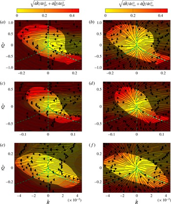
The mean
 $QR$
-phase development is shown by trajectories (black) and by the magnitude of the mean phase velocity (contours) restricted to the pressure term (a,c,e) and the viscous term (b,d,f) of the Navier–Stokes equations, respectively. Three wall-normal locations are shown: (a,b)
 $y^{+}\approx 180$
, (c,d)
 $y^{+}\approx 24$
, (e,f)
 $y^{+}\approx 6.7$
. The bright area covers 95 % of all events and the dashed green lines divide the
 $QR$
-phase space into the four sectors, covering a characteristic local flow topology each.

The second part of the evolution is formed by neglecting all terms except the terms that link the pressure with the velocity gradient tensor (
 $\text{trace}(\unicode[STIX]{x1D643})=\unicode[STIX]{x1D71E}=Q=R=0$
). The part of the evolution caused by the coupling of pressure with the velocity gradient is shown in figure 6(a,c,e) for the three different locations and called restricted pressure evolution in the following. For the outer region the results taken from the present TBL qualitatively match the results taken from the HIT flow of Martin et al. (Reference Martin, Ooi, Chong and Soria1998). The restricted pressure evolution is widely evolving against the restricted Euler flow (figure 1 in Martin et al.
Reference Martin, Ooi, Chong and Soria1998). In the regime of the contracting vortical structures a swirl is formed by the evolution trajectories. The evolution velocity magnitude for this swirling, however, is relatively low. The largest evolution velocity is found in the tail of the teardrop for positive
 $R$
and low values of
 $Q$
as well as in the vortex stretching region, especially for larger values of
 $Q$
. Following the development of the restricted pressure evolution when moving closer to the wall it can be seen that the swirl within the unstable vortex region is ‘unrolling’. The trajectories in this region for
 $y^{+}\approx 24$
point towards positive
 $R$
and the evolution velocity magnitude is increasing. For the location at
 $y^{+}\approx 6.7$
this ‘unrolling’ feature becomes even stronger. The more important effect is that the evolution velocity magnitude is decreasing for the lower left border of the teardrop and for the entire region of the stretching vortical structures. This is already noticeable for
 $y^{+}\approx 24$
, but becomes significant at
 $y^{+}\approx 6.7$
.
The remaining part of the evolution is formed by neglecting all terms except the terms that link the viscous diffusion with the velocity gradient tensor (
 $\text{trace}(\unicode[STIX]{x1D643})=\unicode[STIX]{x1D72E}=Q=R=0$
). The part of the evolution caused by the coupling of viscous diffusion with the velocity gradient tensor is shown in figure 6(b,d,f) for the three different locations and called restricted viscous diffusion evolution in the following. The restricted viscous diffusion evolution in the outer region of the TBL is evolving towards the origin of the
 $QR$
-space. The trajectories are relatively straight, pointing towards the origin and only show a slight counter-clockwise spin. The evolution velocity magnitudes are decreasing with decreasing distance to the origin. For the restricted viscous diffusion evolution no significant changes can be seen when moving closer to the wall. The trajectories develop a slightly stronger spin and the evolution velocity magnitude is decreasing. But overall the restricted viscous diffusion evolution has an invariant character in this TBL flow.
5 Discussion
The evolution of characteristic turbulent structure types is discussed for a compressible turbulent boundary layer with the focus on the change of the evolution for different wall-normal locations.
Comparing the trajectories at all three locations (figure 3
a–c) we find, through visual inspection, that the inward spiralling rate decreases with decreasing distance to the wall. More interestingly, we find a change of the trajectories’ shape that is consistent with the change of shape that we have found for the joint p.d.f.s of
 $Q$
and
 $R$
(Blackburn et al.
Reference Blackburn, Mansour and Cantwell1996; Chong et al.
Reference Chong, Soria, Perry, Chacin, Cantwell and Na1998; Bechlars & Sandberg Reference Bechlars and Sandberg2017). For the outer layer of the TBL they agree qualitatively with experimental results of the outer layer of a TBL (Elsinga & Marusic Reference Elsinga and Marusic2010) and DNS results of a HIT flow (Martin et al.
Reference Martin, Ooi, Chong and Soria1998). The visually identified differences in the inward spiralling strength of the spiralling motions are believed to be caused by two features: (i) as viscous diffusion is driving the dynamics towards the origin in
 $QR$
-space we expect a Reynolds number dependency of the spiralling rate. (ii) The inhomogeneity of the flow, as well as the area of the flow that has been integrated to obtain the statistics representing the mean dynamics in
 $QR$
-space, is strongly influencing the spiralling rates as shown by Lozano-Durán et al. (Reference Lozano-Durán, Holzner and Jiménez2015). As the three cases compared here differ too much with respect to the latter aspect, we see too much uncertainty to allow for a quantitative comparison of the spiralling rates and have to restrict ourselves to the visual investigation for this work.
A discrepancy between the data for the turbulent channel data (Lozano-Durán et al.
Reference Lozano-Durán, Holzner and Jiménez2015) and the present TBL data is that (Lozano-Durán et al.
Reference Lozano-Durán, Holzner and Jiménez2015) found outward spiralling trajectories for statistics being integrated from the wall up to
 $y^{+}=100$
. The present data are integrated over much smaller wall-normal extents, but we could expect outward spiralling trajectories at least in one or more subsets of their integration area to find agreeing results. This is not the case for any of the locations (all tested, but not shown) in the present TBL. On the one hand, this does not necessarily mean that the two results disagree. The different extents of the
 $QR$
-plots for the different locations (here blurred by the scaling) superimposes regions in the
 $QR$
-space that have different characteristics when integrated over larger inhomogeneous extents. This causes difficulties for a direct physical interpretation and could possibly cause behaviours that cannot be seen in a local analysis. On the other hand, this could be a Reynolds number effect. The channel data are at a friction Reynolds number
 $\mathit{Re}_{\unicode[STIX]{x1D70F}}=932$
whereas the present data are taken at a location with a Reynolds number
 $\mathit{Re}_{\unicode[STIX]{x1D70F}}\approx 486$
, which is almost a factor two lower. This is supported by the role of viscous diffusion that drives the dynamics towards the origin in
 $QR$
-space. To discuss this further, comparable integration areas would be needed. This, however, is beyond the scope of this work.
The regions of high and low evolution speed remain at similar locations but vary in magnitude for different wall-normal locations. However, the cycling radii for different wall-normal locations seem to balance the evolution speeds, so that the cycling periods scaled with the local velocity gradient tensor variance do not show significant variations. However the cycling times for the respective locations increase with a decreasing distance to the origin of the
 $QR$
-phase space.
For all locations trajectories forming relatively long straight lines can be found on the lower left side (figure 3
a–c). This indicates that the observed structures first develop within the pure straining structures (III and IV) and then develop a stretching rotational character (I). After developing within the rotational regime the trajectories turn clockwise for all locations. But here first differences for the different locations can be observed. At the outermost location, just like in the case of HIT, the turn is smooth and the trajectories take a long way forming a bump within the unstable vortical structures region (II). In this regime the trajectories turn further until the structures evolve towards the lower left of the
 $QR$
-phase space. Once in the regime of purely straining structures the trajectories develop a sharp clockwise turn towards the evolution direction described at the start, but now much closer to the origin of the phase space. For the locations closer to the wall the initial clockwise turn becomes sharper with the effect that the bump within the unstable vortical structures region decreases. At
 $y^{+}\approx 24$
the bump is still visible, but at
 $y^{+}\approx 6.7$
it has disappeared. At the location closest to the wall we find long, nearly straight trajectories that go from the stretching rotational regime (I) into the contracting rotational regime (II). There is a second sharp turn towards the initial development, but the
 $QR$
-state is now closer to the origin. The sequence of the stages within the evolution period such as vortex creation, stretching and destruction are invariant in polar coordinates in the
 $QR$
-phase-space for the different wall-normal locations (figure 4
d). They take the same angular space at any location but the strengths and ration of the involved terms vary.
It has been established that the strain rate tensor governs the dissipation of kinetic energy, the coupling of both, strain rate tensor and rotation rate tensor, governs the process of vortex stretching and vortex compression (Tsinober Reference Tsinober2000; Hamlington et al.
Reference Hamlington, Schumacher and Dahm2008). For a better understanding of the vortex stretching and vortex compression mechanism, the coupling of the productions of strain and rotation are discussed with respect to the characteristic evolution of turbulence at different wall-normal locations in the TBL (figure 4). Through these plots the successive changes between high enstrophy/strain production events, enstrophy dominated regions, vortex compression events and strain dominated regions along the mean trajectories in
 $QR$
-space highlighted by Luethi et al. (Reference Luethi, Holzner and Tsinober2009) are confirmed for this turbulent boundary flow. Here only the extreme cases at
 $y^{+}\approx 180$
and
 $y^{+}\approx 6.7$
will be discussed as the intermediate location
 $y^{+}\approx 24$
can be seen as intermediate case between the two extremes. Beginning at the start of the blue trajectories in figure 3(a–c) we find that we are in the pure straining regime (
 $\unicode[STIX]{x1D6E5}<0$
) and observe decaying but strong strain production for the outer layer and near-wall region (figure 4
a,c). For the latter this is coinciding with a strong rotation production (figure 4
c). However, as we are in the pure straining regime we know that no vortices are associated with these structures (figure 3
a,c). The structure of the conditionally averaged flow field for this region (Lawson & Dawson Reference Lawson and Dawson2015) indicates that this pure straining region is located in between vortical structures. Following the evolution of the structures in the outer region from this state, we find a strong increase of rotation production and a low production of strain (figure 4
a) which leads to a development of vortical structures which is reflected by changing far into the regime with
 $\unicode[STIX]{x1D6E5}>0$
(figure 3
a). In the near-wall region the relative production of rotation is not much larger than the relative production of strain as it is in the outer region (figure 4
d). Therefore the development into the vortical regime for the near-wall region is not as pronounced as for the outer region (figure 3
a,c). Lawson & Dawson (Reference Lawson and Dawson2015) show that these structure types form coherent regions of fluid in the vortical regime, which supports the idea of elongated vortices. The difference in production for the two locations might be caused by the dense packing of turbulent structures in the near-wall region as well as a direct interaction with the wall itself, in contrast to developing structures being less affected at larger distance to the wall. At both wall-normal locations the structures are evolving into rotation destroying structures. Here the relative rotation destruction in the near-wall region is much stronger than in the outer region of the TBL (figure 4
d). Further, it was noticed that the time that the structures spend destroying rotations is higher in the near-wall region (
 $\unicode[STIX]{x0394}\hat{t}\approx 8$
) than in the outer region (
 $\unicode[STIX]{x0394}\hat{t}\approx 5$
) (figure 4
a,c). As these rotation destroying structures are in the contracting vortical structure regime (
 $\unicode[STIX]{x1D6E5}>0,R>0$
) the increased times explain the increased frequency of occurrence of those structures that Bechlars & Sandberg (Reference Bechlars and Sandberg2017) has identified in the near-wall region (see introduction).
The vortex creation and the vortex stretching processes are strongly dependent on the coupling terms of pressure and the velocity gradient tensor counteracting the nonlinear dynamics, as shown by splitting the evolution of turbulence into its separate parts (figures 5 and 6). This counteraction leads to a development from pure straining structures to vortical structures and allows vortical structures to stretch stably. This mechanism is well developed for the outer layer, but due to changes of the balance of the nonlinear dynamics and the coupling terms of pressure and the velocity gradient tensor in the near-wall region this mechanism becomes more unstable. The stable vortices do not reach as high values of
 $Q$
as they do in the outer region before they become unstable. Again, this might be caused by decreased freedom of spatial development due to dense packing and the presence of the wall in the near-wall region. Further, the wall strongly couples strain and rotation production. While in the outer layer rotation and strain production are well separated, they show the same behaviour at the wall. This means on average every vortex that is created is associated with a strongly strain growing in a similar, just slightly weaker, way as its rotation field in the near-wall region.
Similarly to the vortex creation and vortex stretching, strain and rotation production are more closely coupled in the near-wall region for the unstable vortical regime where rotation is destroyed (II). Whereas this process is widely uncoupled to the strain production in the outer region (figure 4
a), the decreased distance to the wall associates the strain destruction with rotation being destroyed (figure 4
c). But here we find slightly less strain than rotation being destroyed. In parts of the regime for unstable vortices the coupling terms of pressure and the velocity gradient tensor change the character strongly with varied distance to the wall (figure 6
a,c,e). The consequence of this is that the evolution of turbulent structures in this regime is changed strongly in the near-wall region which causes a different characteristic composition of turbulence, reflected by the changed joint p.d.f. of
 $Q$
and
 $R$
. In the regime of unstable vortical structures the ‘unrolled’ swirl of the restricted pressure evolution (figure 6
e) has the effect that the trajectories of the overall evolution extend much further towards the lower right for the near-wall region than for the outer region of the TBL. This causes the much lower inwards spiralling rate that we found for the evolution in the near-wall region (figure 3
c). A second effect of this is that the tail of the teardrop shaped joint p.d.f. of
 $Q$
and
 $R$
vanishes in the near-wall region (see Bechlars & Sandberg (Reference Bechlars and Sandberg2017), for the varied
 $QR$
-plot shape).
6 Conclusions
In order to obtain insight into the development of turbulence in compressible flows the compressible Lagrangian dynamics of the first three invariants of the velocity gradient tensor
 $P$
,
 $Q$
and
 $R$
have been derived. With this novel set of equations the evolution of characteristic turbulent structure types have been studied in a compressible turbulent boundary layer. The focus in this study was on the change of the evolution for different wall-normal locations.
The mean evolution for the velocity gradient tensor invariants was found to vary strongly with the distance to the wall. Based on the changes of this evolution the previously stated variations of the
 $QR$
-plots in a TBL (see Blackburn et al.
Reference Blackburn, Mansour and Cantwell1996; Chong et al.
Reference Chong, Soria, Perry, Chacin, Cantwell and Na1998; Bechlars Reference Bechlars2015) have been explained with the change of turbulence evolution in a TBL.
The role of the viscous diffusion in the overall evolution in the
 $QR$
-phase space is relatively simple. It drives all structures towards the origin and its strength in doing this is increasing with the distance to the origin. This is plausible as the gradient magnitudes in the flow increase with increasing distance to the origin. Further, the features of viscous diffusion are relatively invariant in this flow and are therefore not the main cause for the observed variations in the overall evolution (figure 3). Therefore viscous diffusion does not appear to be very important for the changes of the turbulence evolution of turbulence in this flow.
The coupling of the pressure Hessian with the velocity gradient that is affected by the wall drives nearly all the changes of the invariant dynamics that we have discussed in this work. Most significantly, it changes the inward spiralling rate as well as the shapes of the trajectories and therefore the changes of the
 $QR$
plots. The importance of the pressure–velocity gradient relation that we have discovered for the changes of the turbulence dynamics in the present flow is believed to be of significant relevance for all turbulent flow. From a
 $QR$
-analysis perspective it appears to be the most significant feature that affects the turbulence development. This needs to be shown also for other flows, but the methodology to investigate other flows is provided within this work.
Despite all the observed changes, the general mean lifecycle of turbulent structures stays unchanged in the
 $QR$
-space. The sequence ‘straining structures develop to stretching vortical structures and further to contracting vortical structures before the lifecycle continues again in the straining structures’ is invariant within the present turbulent boundary layer flow.
The slowed down evolution velocity of vortical structures in the near-wall region is the cause for the strongly increased frequency of occurrence of this structure type observed for a TBL in previous work.
Lastly, the wall has a coupling effect on the strain rate magnitude production and the rotation rate magnitude production. In the near-wall region an increase of rotation energy is in a mean sense always associated with an increase of strain energy and vice versa.
Acknowledgements
Funding through EPSRC grant EP/I003754/1 is acknowledged. Computer time was provided by the UK Turbulence Consortium under EPSRC grant EP/L000261/1. This work used the UK Research Data Facility (http://www.archer.ac.uk/documentation/rdf-guide).