Did imperialism pay? Many modern economic historians have been skeptical of this claim. Edward Fitzgerald, for example, argued that France's colonial empire provided no net economic benefit to the mother country, even absent the cost of the colonial wars of the 1940s and 1950s.Footnote 1 Lance Davis and Robert Huttenback argued that Britain gained little from its colonial empire—private returns from Imperial investments declined substantially after 1880—and were in any case dwarfed by the subsidies that U.K. taxpayers paid to administer and defend the colonies.Footnote 2 Michael Edelstein found much the same in his analyses of British imperialism.Footnote 3
The economic benefits to the United States of American imperialism have not been exempt from similar skepticism. Even the most canonical case of economically motivated imperialism—the U.S. intervention to secure Panama's independence and construct a canal under American sovereignty—has come under doubt. Stanley Lebergott, for example, noted that the canal “gave equal advantage to any nation that chose to use the Canal,” and the benefits to shipping accrued “in the same proportion as American railroads were injured.”Footnote 4 A 1929 analyst agreed with Lebergott's assessment, pointing out that, “Transcontinental railroads, intermountain jobbers, manufacturers and distributors of the Middle West, exporters on the Pacific coast, and others are positive in pointing out serious losses which they have incurred because of Canal competition,” arguing that any gains derived from large implicit subsidies to the canal.Footnote 5 Earlier observers concurred. A British engineer working for Colombia, J. T. Ford, wrote in 1903, “For the United States [the Panama Canal] is a paying concern not from a commercial standpoint—it will therein be a loser—but on account of its Navy.”Footnote 6
Boosters of the Panama Canal, however, had no such doubts. In the 1850s, a group of U.S. investors constructed a railroad across Panama, then a province of Colombia. As a witness told a Senate committee in 1849, the railroad was meant to pave the way for a canal “by showing to the world how immense this business is.” The railroad proved to be phenomenally profitable.Footnote 7 In 1878 a prominent Wall Street analyst estimated that an Isthmian canal would save world shipping $48 million per year, of which $36 million would accrue to the United States.Footnote 8 Two years later, President Rutherford Hayes declared, “The policy of this country is a canal under American control. Our commercial interest is greater than that of any other country.”Footnote 9 An estimate delivered to Congress in 1903 concluded that a canal would produce a stream of benefits which when capitalized would be worth $1.2 billion, or 4.7 percent of U.S. GDP.Footnote 10
We argue that the boosters of an isthmian canal had it right; the Panama Canal produced substantial benefits for the consumers of transportation during its first quarter century of operation. Our minimum estimate of the social rate of return is well in excess of the returns from U.S. government bonds. The lion's share of those social returns from the canal accrued to the United States. In fact, the lion's share of the benefits originated from the transportation of petroleum products from California to the East Coast. In other words, for the United States, the Panama Canal paid.
We also argue that the United States managed to leverage its military prowess into a far better deal than it otherwise could have negotiated. The 1903 agreement made with the newly independent Republic of Panama (under the threat of intervention and with thousands of U.S. troops on Panamanian soil) granted the United States a far higher share of the canal's economic benefits than earlier agreements negotiated between the French-owned New Panama Canal Company and Colombia, or between the United States and Nicaragua. In fact, the 1903 agreement with Panama granted the United States a higher share of the benefits than a 1902 American offer that the Colombian government had rejected. The United States even succeeded in getting Panamanian taxpayers to subsidize some of the overhead costs of canal construction and operation.
THE PANAMA CANAL AND WORLD COMMERCE
The first step in evaluating the economic benefits of the Panama Canal for the United States is to produce an estimate of the commercial benefits of the Panama Canal for world commerce. Such an estimate depends upon three variables. The first is the cost of constructing and operating the Panama Canal. The second is the reduction in the cost of transportation induced by the opening of the canal. The third is the sensitivity of shippers to the cost of transportation. We take each of these three factors in turn.
The Costs of the Panama Canal
The Panama Canal was the most expensive public works project in American history up until that time. Between 1903 and 1914, the United States spent $326 million directly on Panama Canal construction, or $6.3 billion in 2006 dollars using the U.S. GDP deflator.
The canal exceeded its estimated construction cost by a considerable margin. A 1902 congressional committee authorized the project based on a cost projection of $144 million.Footnote 11 As early as 1905, however, the New York Times complained that the Isthmian Canal Commission was on track to have spent $66 million by the end of the year, with “no dirt flying.”Footnote 12 By the time initial construction finished in 1914, construction costs surpassed initial estimates by a factor of 2.3. The scale of Panama Canal cost overruns, therefore, was significantly higher than on comparable projects such as the Erie Canal (1.5), Hoover Dam (1.1), or the Bay Area Rapid Transport system (1.6), although Panama Canal cost overruns did compare favorably to Boston's infamous Big Dig (5.2 and counting).Footnote 13 Work continued for six more years as a result of unexpected landslides, and the canal did not fully open to civilian traffic until 12 July 1920.Footnote 14 The Isthmian Canal Commission expended an additional $46 million during that period, driving the scale of overruns to 2.6 times the initial estimate.
Construction costs were not the only startup costs of the canal. The United States made an initial outlay of $40 million to purchase the assets of the French-incorporated New Panama Canal Company and an additional $10 million to obtain the rights to the Canal Zone from the Panamanian government.Footnote 15 The United States also incurred an implicit interest cost during construction, which we calculated using the yield on long-term U.S. federal bonds. For each year between 1903 and 1914, we took the cumulative amount spent on construction and payments to the New Panama Canal Company and the Panamanian government, and then multiplied the cumulative amount by the interest rate in order to determine the implicit interest cost. In addition, we included the $25 million paid to Colombia in 1921 as part of the canal's startup costs. Lastly, we converted the startup costs for each year into 1925 dollars using the U.S. GDP deflator. Aggregate startup costs came to $788 million in 1925 dollars.Footnote 16
The United States also needed to defend the canal, which required the construction of barracks, shore defense batteries, and naval support facilities. However, the initial proposal envisioned no special expenditures for defense. The Canal Commission believed that the canal was essentially indefensible, because “a small party of resolute men, armed with a few sticks of dynamite, could temporarily disable it without great difficulty.” In addition, if an enemy fleet could dominate the Caribbean, then the canal would be strategically worthless. The commission, therefore, recommended “neutralization.”Footnote 17
The Taft Administration rejected neutralization in 1909. Military needs expanded to include a permanent garrison, coastal batteries, and, eventually, air defense.Footnote 18 We obtained the cost of defense-related construction from the Annual Report of the Governor of the Panama Canal. Using the same procedure outlined above, we calculated the total cost of defense-related construction (including air defense and antiship artillery and a three month supply of ammunition) to be $158 million in 1925 dollars, including the implicit interest expense.
In order to come up with an estimate of the total startup cost of the Panama Canal, we added $125 million in defense-related construction to our estimate of $788 million in other costs, for a total of $946 million in 1925 dollars. When adjusted using the GDP deflator, $946 million in 1925 dollars is the equivalent of $9.1 billion in 2006 dollars. A better sense of the canal's scale, perhaps, is given by comparing the startup costs relative to resources available to the United States during its construction. The total startup costs came to approximately 1.8 percent of the country's 1903 GDP, albeit spread over 18 years between 1903 and 1921. An equivalent share of the United States' nominal GDP in 2006 would total $242.5 billion.Footnote 19
Transportation Cost Savings of the Panama Canal
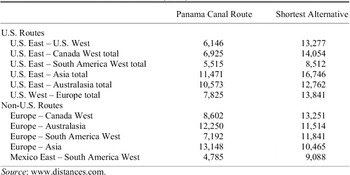
The Panama Canal's chief benefit to world trade came from shortening distance. Without it, trade between the American West Coast and the American East Coast or Europe had three options: travel via the transcontinental railroad, travel by ship to Mexico or Panama and then along the Tehuantepec or Panama railroads to be unloaded again onto another ship, or travel by ship around the southern tip of South America.Footnote 20 The canal also cut shipping distances between Europe and the West Coast of South America. (See Table 1 for representative distance comparisons.) The canal had little impact on shipping distances between Europe and Asia or the Antipodes, which could travel via alternate routes.

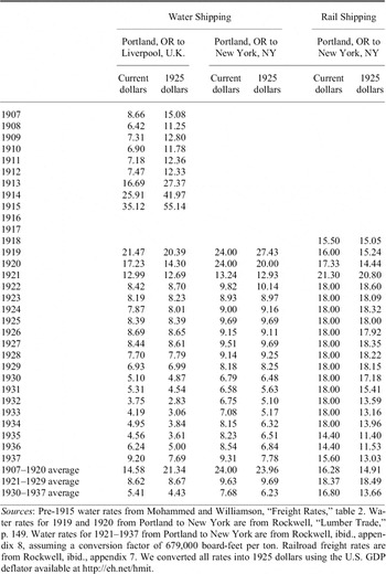
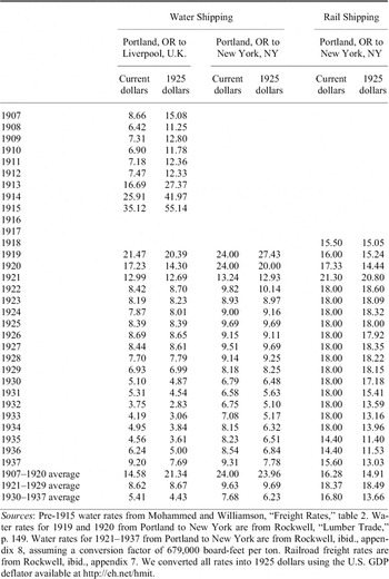
How large were the social savings engendered by the Panama Canal? (See the model in the Appendix.) Saif Mohammed and Jeffrey Williamson have compiled a series of shipping costs between Portland, Oregon, and Liverpool, England. Their data are reproduced in Table 2. In 1921, the canal's first full year of operation, shipping costs dropped 11 percent. In 1922, the canal's second year of operation, shipping costs dropped a further 31 percent below their pre—World War I level. Since the Panama Canal reduced the distance between Portland and Liverpool by 42 percent, it seems likely that the canal caused the lion's share of the fall in freight rates.
TRANSPORTATION RATES PER TON
Sources:
Pre-1915 water rates from Mohammed and Williamson, “Freight Rates,” table 2. Water rates for 1919 and 1920 from Portland to New York are from Rockwell, “Lumber Trade,” p. 149. Water rates for 1921–1937 from Portland to New York are from Rockwell, ibid., appendix 8, assuming a conversion factor of 679,000 board-feet per ton. Railroad freight rates are from Rockwell, ibid., appendix 7. We converted all rates into 1925 dollars using the U.S. GDP deflator available at http://eh.net/hmit.
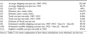
If the drop in freight rates in 1921/22 was due to the shorter travel distance that the canal made possible, then the per-mile transportation cost should not have changed when the canal opened. In fact, per-mile shipping costs rose slightly.Footnote 21 The reason is that part of the cost of transporting a ton of cargo does not vary with distance: loading and unloading, warehousing, insurance, docking fees, and so on. We estimated this fixed cost of shipping by solving the following pair of equations with two unknowns

We ended up with an estimate of a fixed cost per ton of $3.12 in 1925 dollars.Footnote 22 (See Table 3.) The variable cost of transporting a ton one mile, therefore, was roughly 0.07¢ (U.S.) in 1921/22.
FIXED AND VARIABLE SHIPPING COST ESTIMATES, PORTLAND, OREGON TO UNITED KINGDOM (1925 dollars)

Source:
Table 2. For more explanation of how these calculations were obtained, see the text.
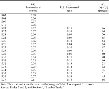
We estimated shipping costs per ton-mile by subtracting our estimate of fixed costs from the total cost per ton-mile. Because the United States required that all intercoastal shipping be carried by U.S. flagged vessels, intercoastal transport was significantly more expensive per ton-mile than international shipping. We therefore calculated costs per mile separately for intercoastal and international routes.
We then calculated the social savings generated by the opening of the canal under three assumptions. First, we assumed that the opening of the Panama Canal had no effect on the fixed cost of shipping. This assumption matches those of contemporary observers, who claimed that insurance rates did not differ between the Cape Horn and Panama Canal routes.Footnote 23 If, however, this assumption is incorrect and the fixed costs actually fell, then our estimates of the cost savings will be biased downward.
Second, we assumed that all of the reduction in per-mile shipping costs after 1921 came from improvements in shipping technology or drops in the cost of inputs such as fuel and labor. We do not attribute them to the opening of the canal. This assumption also biases downwards our estimates of the canal's cost savings.
Third, we assumed that intercoastal cargoes would be shipped via the transcontinental railroad in the absence of the Panama Canal, as transcontinental freight rates were lower than transcontinental shipping costs before the canal opened. Because we do not have data on the value of the cargoes transiting the canal, we do not take into account savings in inventory costs due to lowered time in transit, which further biases downwards our estimates.
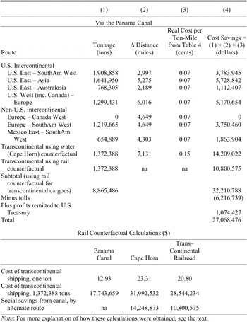
We include a representative calculation of the social savings from the canal for the year 1921. The Panama Canal administration collected tonnage and route data on all cargoes passing through the canal. They aggregated the data into 11 routes, recording it separately for each direction.Footnote 24
For each aggregated route, we calculated representative distances, both using and not using the Panama Canal, selecting specific city pairs on the basis of evidence from the official canal reports.Footnote 25 Alternative choices, for example Manila instead of Shanghai, or Baltimore instead of New York, did not affect distances by more than 10 percent.
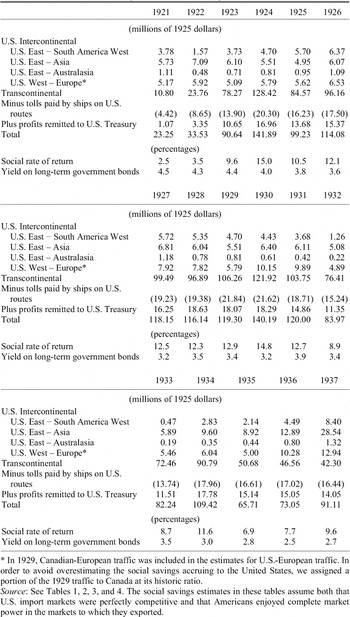
We calculated the basic social savings as follows. For each route, we multiplied the number of tons shipped along that route by the reduction in distance caused by the opening of the Panama Canal, giving us the reduction in the number of ton-miles that needed to be shipped in order to move the same amount of cargo between the same ports. To calculate the value of the social savings, we multiplied the reduction in the number of ton-miles by the real variable cost of shipping per ton-mile (in 1925 dollars) from Table 4. In effect, this method weighted each route by the volume of cargo passing through the canal and the difference in the distance created by the opening of the canal. (Given the lack of distance reduction and the almost negligible quantity of cargoes moved through the canal along the Europe-Asia and Europe-Australasia routes, we assumed that there were no savings caused by the Panama Canal on those routes.) We then subtracted the tolls charged by the canal and added back canal profits remitted to the U.S. Treasury, in order to net out operating costs. This avoided miscounting resources consumed in the operation of the Panama Canal as social savings.
ESTIMATED VARIABLE SHIPPING COST PER TON-MILE IN 1925 DOLLARS

Note:
These estimates use the same methodology as Table 3 to strip out fixed costs.
Source:
Tables 2 and 3; and Rockwell, “Lumber Trade.”
Calculating the social savings from U.S. transcontinental cargoes required a somewhat different method. In the absence of the Panama Canal, the transcontinental railroad would be less expensive for most such cargoes than shipment around Cape Horn. However, while the railroad route had a significantly higher cost per ton-mile, it was shorter than the canal route, making a simple difference calculation untenable. Instead, we used the costs reported by Arthur Rockwell of transporting a ton of freight from Portland, Oregon, to New York by the canal and by the transcontinental railroad.Footnote 26 We first converted those costs into 1925 dollars using the GDP deflator. We then multiplied the costs by the number of tons of cargo actually shipped through the canal along the transcontinental route. Finally, in order to calculate the social savings, we subtracted the total cost of shipping goods via the canal from the total cost of using the railroad. In order to check our results, we also computed the cost of shipping goods via the Cape Horn route using the data in Tables 1, 3, and 4. Unsurprisingly, given that transporters overwhelmingly preferred the railroad, the Cape Horn route proved to be more expensive.Footnote 27 (See Table 5.)
SOCIAL SAVINGS CALCULATION FOR 1921, ASSUMING ZERO ELASTICITY

Note:
For more explanation of how these calculations were obtained, see the text.
It might be argued that in the absence of the Panama Canal, the additional traffic on the American railroad system would have burdened the existing infrastructure and required investment in new rolling stock and new track, thus raising freight costs. However, between 1921 and 1929, while ton-miles transported on U.S. railroads increased 45 percent, the inflation-adjusted price of rail transport per ton-mile decreased by 13 percent.Footnote 28 This implies the United States could have further expanded its railroad freight capacity without significantly driving up the cost of rail transport per ton-mile. Even so, should this assumption be incorrect, and railroad freight rates would have risen in the absence of the Panama Canal, it would only serve to increase our estimates of the social savings.
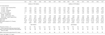
Did the transportation cost savings produced by the Panama Canal justify the high construction cost? In order to answer this question, we divided the social savings estimates (in 1925 dollars) by the canal's total startup cost (also in 1925 dollars) in order to produce a “social rate of return.” The social rate of return, as we have defined it, measures the aggregate of the flow of benefits to the owners of the canal (for example, the U.S. Treasury) and the users of the canal's services. If those returns are lower than the opportunity cost of capital, then the Panama Canal did not add value to the world economy. We take the rate of return on U.S. federal bonds to represent the returns from the risk free alternative use of capital—paying down the national debt. In 1921, the canal's first full year of operation, the estimated social rate of return was 2.9 percent, less than the inflation-adjusted rate on U.S. federal 10-year bonds.
The social rate of return on the Panama Canal did not remain low for long. By 1923 it exceeded 10 percent, far above the rate of return on U.S. government bonds, and it remained above that level until 1932. Even at its post-1923 nadir, in 1935, the social rate of return never fell below 7.7 percent. (See Table 6.)
BASIC GLOBAL SOCIAL SAVINGS ESTIMATES, BY ROUTE

Source:
See Tables 1, 2, 3, and 4.
Demand Elasticity of Transportation
The lion's share of the domestic cargo passing through the canal consisted of petroleum from Southern California and lumber from the Pacific Northwest. Both products had substitutes that did not need the canal: Venezuelan oil and Southern pine lumber. Much the same can be said of international cargoes, such as Philippine sugar or copra, both of which had domestic substitutes. Because of the availability of substitutes, the demand for transporting these products may have been sensitive to shipping costs. The more sensitive demand was to shipping costs, the lower the true social savings from the canal.
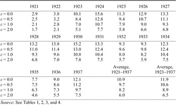
Our calculations in Tables 5 and 6 assumed that transportation demand was insensitive to shipping costs—in other words, that the price elasticity of transportation demand was zero. We have redone the calculations for different assumptions about the price elasticity of demand for transportation via the canal. We computed the ratio (Sε/S 0) between the social savings at a given price elasticity (S ε) and the social savings when the price elasticity is zero (S 0) using the following two equations,


where φ is the ratio between the cost of transport without the use of the Panama Canal and the cost of transport using the Panama Canal and ε is equal to the price elasticity of demand.Footnote 29 Because the proportional cost savings of the canal were different for every route, we calculated the change in the cost savings for various demand elasticities separately for every route and then aggregated upwards.
Assumptions about price elasticity could have potentially large effects on cost savings. A price elasticity of 0.5 (in line with other studies of the social savings from transportation) would reduce savings by approximately 15 percent. A price elasticity of 1.0 would reduce savings estimates by a quarter, and an elasticity of 2.0 would roughly cut them in half.
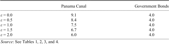
Do the results in Table 6 depend on the assumption of inelastic demand? We recalculated the social rate of return assuming demand elasticities ranging from 0.5 to 2.0. Even at the extreme assumption of a demand elasticity of 2.0, the average social savings generated by the canal, as a percentage of the Panama Canal's total construction cost, remain well in excess of the 4.2 percent real return on federal government bonds during the period. In short, inasmuch as the rate of return on U.S. government bonds proxies the opportunity cost of capital, then the canal generated significant savings for the world economy during the 1920s (See Table 7).
GLOBAL SOCIAL RATES OF RETURN FROM THE PANAMA CANAL FOR ALTERNATIVE VALUES OF THE PRICE ELASTICITY OF DEMAND FOR FREIGHT SERVICES VIA THE CANAL (percentages)

Source:
See Tables 1, 2, 3, and 4.
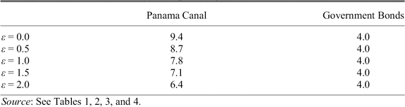
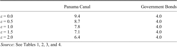
An alternative way to compare the social returns generated by the Panama Canal with the returns that could be generated by buying back government debt is to calculate an “internal rate of return,” or IRR, for the Panama Canal project. The IRR is the discount rate at which the net present value of a series of cash flows is equal to zero. It can be used to compare the returns available from different projects with different patterns of outlays and revenues. Table 8 calculates the inflation-adjusted IRR for the Panama Canal, starting from the first outlays in 1904 and treating the social savings from the canal as the equivalent of positive cash flows. It also calculates the IRR from investing the same amount (over the same period) in government bonds. Even at an elasticity of 2.0, the IRR for the Panama Canal is more than 50 percent higher.
INTERNAL RATE OF RETURN: BASE YEAR = 1904 (percentages)
Source:
See Tables 1, 2, 3, and 4.
THE PANAMA CANAL AND THE AMERICAN ECONOMY
The American politicians who backed the creation of the Panama Canal did not do so in order to benefit global commerce. The goal of the politicians who backed the canal was the stimulation of American commerce and the capture of the canal's benefits by American producers and consumers. In fact, both the Taft and Wilson Administrations tried to mandate that the canal would charge no tolls on intra-U.S. traffic, and only backed down under intense pressure from the United Kingdom. The United States agreed to charge the same tolls and grant the same access to American and foreign flagged vessels. The United States also agreed to refrain from discriminating between vessels bound to U.S. ports and vessels traveling purely international routes, although Washington prevented foreign warships from passing through the canal.Footnote 30
Geography, nevertheless, insured that the United States would reap most of the benefits from the Panama Canal, despite the U.S. failure to discriminate in favor of American commerce. The fact that the U.S. possessed economic centers on both coasts meant that the canal carried much of the U.S. East Coast's trade with Asia and the West Coast's trade with Europe, as well as a significant amount of intra-U.S. commerce. In fact, intra-U.S. transcontinental traffic averaged 41 percent of the cargo passing through the canal (by tonnage) in 1923–1937. (Cargo originating in U.S. ports made up 19 percent, while cargo terminating in U.S. ports made up an additional 15 percent over the same period. Only 25 percent of all cargo passing through the canal traveled non-U.S. routes.) Table 9 presents the basic estimates of the social savings generated by the canal for routes originating or ending in the United States. Toll costs include only the tolls paid on these routes. Canal profits remitted to the U.S. Treasury, however, include the profits generated from ships passing between non-U.S. ports, since such profits ultimately benefited American taxpayers.
BASIC AMERICAN SOCIAL SAVINGS ESTIMATES, BY ROUTE (millions of 1925 dollars)

* In 1929, Canadian-European traffic was included in the estimates for U.S.-European traffic. In order to avoid overestimating the social savings accruing to the United States, we assigned a portion of the 1929 traffic to Canada at its historic ratio.
Source:
See Tables 1, 2, 3, and 4. The social savings estimates in these tables assume both that U.S. import markets were perfectly competitive and that Americans enjoyed complete market power in the markets to which they exported.
The estimates in Table 9 assume that Americans captured the cost savings generated by the canal regardless of whether the origin or destination of the cargo was in the United States. If U.S. import markets were perfectly competitive, then foreign exporters to the United States would pass on cost savings to American consumers. Similarly, if American exporters were monopolists, then they would capture the drop in transportation costs. Table 9 implicitly assumes that both conditions held; U.S. import markets were perfectly competitive, while Americans enjoyed complete market power in the markets to which they exported. That is to say, Table 9 assumes that the canal caused a drop in the CIF prices faced by American consumers of imports equal to the fall in transport costs, and simultaneously assumes that the opening of the canal raised the free on board (FOB) prices received by American exporters by an amount equal to the drop in transport costs. This assumption is unlikely. The estimates of the returns to the United States in Table 9, therefore, are overestimates.
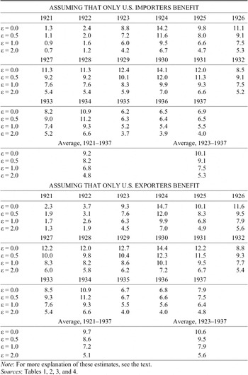
The estimates presented in Table 10 correct for this overestimation. The first set of estimates assumes that the cost savings from the opening of the canal were passed on to consumers. U.S. consumers, under this assumption, enjoyed lower CIF import prices after the canal opened equal to the transportation cost reduction engendered by the canal. This same assumption, however, implies that U.S. exporters received no benefits from the opening of the canal. Consumers in other countries enjoyed lower CIF prices for U.S. exports (and thus captured the social savings produced by the canal), while U.S. producers received the same FOB prices as before. The first set of estimates, therefore, include the social savings on transcontinental cargoes (for which it does not matter who captured the social savings, since both producers and consumers were presumably American) and international cargoes which terminated in the United States.
AMERICAN SOCIAL RATES OF RETURN FROM THE PANAMA CANAL FOR ALTERNATIVE VALUES OF THE PRICE ELASTICITY OF DEMAND FOR FREIGHT SERVICES VIA THE CANAL (percentages)

Note:
For more explanation of these estimates, see the text.
Sources:
Tables 1, 2, 3, and 4.
The second set of social savings estimates in Table 10 assumes the reverse, that producers (both foreign and domestic) captured all the savings engendered by the opening of the canal. The assumption, in other words, is that the opening of the canal did not cause the CIF prices faced by American consumers to change. Rather, the savings were captured by foreign producers and shippers. At the same time, the FOB prices received by American exporters rose by an amount equal to the canal's transportation cost savings, and American export producers, not foreign consumers, captured the social savings created by the canal. The second set of estimates, therefore, includes the social savings on transcontinental cargoes and international cargoes which originated in the United States.
Because the United States was a net exporter, the first set of estimates in Table 10 (which assume that import consumers captured the social savings) are slightly lower than the second set (which assume that export producers captured the social savings). Both estimates are, of course, lower than the estimates presented in Table 9. Nonetheless, even the lowest estimates in Table 10 are well above the rate of return on U.S. government bonds.
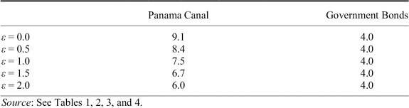
We also repeated the calculations for the Panama Canal's IRR (see Table 8) using our lowest estimate of the social savings captured by the United States from Table 10. These calculations, shown in Table 11, indicated that the canal was a better use of government funds than buying back government debt, even at unrealistically high demand elasticities.
INTERNAL RATE OF RETURN, ASSUMING THAT ONLY U.S. IMPORTERS BENEFIT: BASE YEAR = 1904 (percentages)
Source:
See Tables 1, 2, 3, and 4.
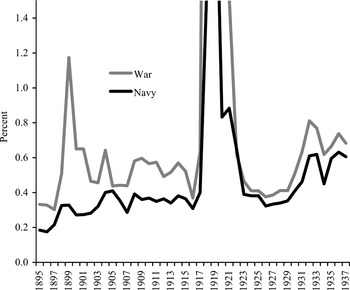
Did the Panama Canal generate defense-related savings for the United States? In terms of naval expenditures, the canal appears to have been a wash. Its opening to military vessels in 1914 did not allow the United States to reduce its naval presence in the Caribbean, since the canal would prove useless in the event that the United States lost naval superiority in the region. Navy strategists, meanwhile, continued to maintain that the United States needed to maintain a separate (and even larger) force in the Pacific in order to defend American interests in Hawaii and the Philippines.Footnote 31 In addition, the canal's locks could not handle the newest class of battleship. In 1916, therefore, Congress committed to building a two-ocean navy, but this commitment did not outlast the end of the First World War.Footnote 32 Congress soon cancelled its commitment to a two ocean navy. Rather, Congress ratified the Washington Treaty of 1922, which obviated the need to build either large battleships or a two ocean fleet—at least until the treaty expired in 1936. The U.S. Navy met its commitment to the Caribbean by shifting resources from the North Atlantic and Pacific, rather than by expanding the fleet. Naval spending fell back to prewar levels by 1923 (see Figure 1). Inasmuch as the existence of the Panama Canal encouraged the United States to sign the Washington Treaty and thereby limit its naval expense, the canal may have provided additional defense-related savings to the American economy. Whether such savings were prudent considering subsequent events is, of course, an entirely different question.
WAR AND NAVY DEPARTMENT SPENDING AS PERCENTAGE OF GDP

Did the Panama Canal generate nonnaval direct defense costs high enough to offset the social savings that it generated for the U.S. economy? The reports of the Governor of the Canal Zone contained figures for capital expenditures on defense-related construction, including the installation of fixed weapons systems such as antiaircraft guns and antiship artillery. Such expenses, therefore, are accounted for as costs in our social savings estimates. The garrison's operating costs, however, are not accounted for. We therefore employed two methods to estimate the operating costs of the Canal Zone garrison. The first assumed that the soldiers and material in the Canal Zone would be redeployed elsewhere in the absence of the canal. We thus turned to the Annual Reports of the Secretary of War and the records of Senate hearings on War Department appropriations in order to estimate the direct costs of the Panama Canal garrison. Such costs averaged only $350,000 (in 1925 dollars) over 1922–1937—too little to have any appreciable effect on our estimates of the social savings produced by the Panama Canal.Footnote 33
The second way in which we estimated defense costs assumed that all soldiers would be demobilized and nonspecialized equipment decommissioned in the absence of the Panama Canal. The 1923 Senate appropriations hearings provided estimates of the total cost of clothing, equipping, paying, provisioning, sheltering, and transporting an Army with varying end strengths of 122,000, 132,000, and 156,000 soldiers. These figures allowed us to calculate the marginal cost of equipping, sustaining, and deploying an additional soldier. In most categories, unsurprisingly, the marginal cost was less than the average cost, but there were a few cases in which lumpy expenditures (notably for water and sewage provision and railroad transportation) led to significantly rising marginal costs.Footnote 34 We then multiplied the marginal cost per soldier by the size of the Panama Canal garrison (which averaged 10,395 officers and enlisted men in 1922–1935) and added in all special appropriations for Canal Zone defense. Using this methodology, we created a high estimate of the average operating cost of Canal Zone defense in 1922–1935 of $10.4 million (in 1925 dollars). The high estimate of defense costs reduced the base social savings estimates between 8 and 18 percent, depending on the year.Footnote 35 While appreciable, the high estimate was not enough to offset the social savings the canal generated for the U.S. economy.
Did the Panama Canal raise indirect defense costs? The Roosevelt Corollary of 1904 committed the United States to insuring the political and financial stability of the Circum-Caribbean. It is unclear, however, that the need to defend the canal drove U.S. interventionism.Footnote 36 Even if it had, it is not clear that U.S. interventions imposed a significant additional cost on the Treasury. Between 1903 and 1916, the United States intervened in Cuba (twice), Honduras, Mexico (twice), Nicaragua, the Dominican Republic (twice), and Panama itself outside the Canal Zone (twice)—but War Department spending (whether measured in constant dollars or as a percentage of GDP) did not rise appreciably.Footnote 37 (See Figure 1). The reason is that the United States required the nations that it occupied to pay most occupation costs out of current revenues or bonds issued in the name of the occupied country, not the United States. The sustained rise in War Department spending that took place after the Spanish-American War was due to the need to maintain a large military presence in the Philippines, rather than the Caribbean—and while the U.S. possession of the Philippines may have influenced the decision to build the Panama Canal, the Panama Canal did not affect the decision to annex the Philippines. The post-1930 rise in War Department spending, meanwhile, coincided with President Herbert Hoover's public disavowal of armed intervention in the Americas and the withdrawal of remaining U.S. troops from Haiti and Nicaragua.
DIVIDING THE RENTS: PANAMA AND THE UNITED STATES
Due to its geographic position, the United States stood to gain a larger share of the canal's benefits than other countries. By the same token, however, any government or private entity that controlled the isthmus stood to extract substantial rents from American users of transportation services. The Isthmus of Panama enjoyed a unique geographic asset, its location. While other potential canal locations existed, geographic and political obstacles made them inferior. (A private 1887 attempt to build a canal in Nicaragua ran into technical difficulties in dredging the San Juan River and abandoned construction in 1893.)Footnote 38
Given the size of the social savings created by the canal and the isthmus's privileged geographic position, one might expect that the owners of the Isthmus of Panama would have leveraged this position into a lucrative deal. For example, its owners might have extracted those rents by charging the United States a high price for the right to build the canal—as Colombia tried to do when it controlled the Isthmus. More generally, a private or non-U.S. canal operator could have set shipping rates at a significantly higher level than the United States chose to charge. Worse yet from the American point of view, a non-American canal operator might have been able to price discriminate among users and extract even more rents from U.S. commerce.
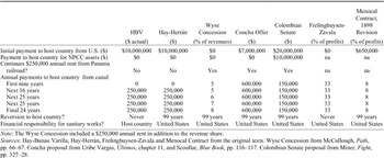
In fact, however, the Hay-Bunau-Varilla (HBV) Treaty which set the terms of U.S. payments for the use of Panama's territory transferred remarkably few resources to the Panamanian government. The reason is that the United States used military force or the threat of military force to obtain a better deal for itself than it could have otherwise obtained. When Colombia balked at U.S. terms for a canal treaty, the United States first sent Marines to occupy the Panama Railroad, and then prevented the Colombian government from halting Panama's secession. When the Panamanian government in turn balked at the United States' revised demands, the United States sent 2,000 additional Marines to Panama and threatened the new government with “grave consequences” if it did not sign.Footnote 39
In order to quantify the benefits the United States gained from its intervention in Panama, we need to determine how much the owners of the isthmus would have obtained from a counterfactual agreement that did not involve the threat of military force. Fortunately, we have identified six such counterfactual agreements. They consist of the U.S. treaty proposal rejected by the Colombian senate in 1903, two Colombian offers made the United States during the 1902/03 negotiations, the 1873 agreement that Colombia signed with Ferdinand de Lesseps to construct an isthmian canal, and the terms of two agreements struck with Nicaragua in 1884 and 1898. In all cases, the counterfactual agreements would have provided the owner of the isthmus with a substantially higher share of the economic benefits than did the actual HBV Treaty.
The Factual
The 1903 agreement that created the Panama Canal involved American threats of force first against Colombia, and then against the newly created Republic of Panama. The United States opened negotiations with Bogotá in 1902. The United States demanded the perpetual cession of a ten-mile-wide band around the canal, to include Colón and Panama City.Footnote 40 Ambassador José Vicente Concha countered with a 99-year lease on a six-mile zone that would not include Colón or Panama City. In return, he demanded an upfront payment of $7 million and an annual rent of $600,000. He also insisted that “neither national, local, departmental, nor any other sort of tax on the canal be prevented.”Footnote 41 Concha believed Colombia was in a strong negotiating position. First, an 1887 attempt to construct a Nicaraguan canal had foundered on engineering difficulties in dredging the San Juan River.Footnote 42 Second, the United States had already agreed to pay $40 million for the Panamanian assets of the French-incorporated New Panama Canal Company (NPCC). The NPCC had obtained those assets under an 1878 concession that was due to expire in 1903, which meant that Colombia would have a claim on the $40 million in the event that no agreement was reached.Footnote 43
The United States responded to Concha by sending Marines to occupy trains passing along the Panama Railroad. Concha abruptly returned to Colombia. “In no case, for any human reason, will I sign any treaty with the government of the United States while its troops continue to occupy Colombian territory against every principle of justice and in violation of a public promise.”Footnote 44 The Colombian chargé d'affaires, Tomás Herrán, took over the negotiations.Footnote 45 The resulting Hay-Herrán Treaty granted the U.S. a 99-year lease on a six-mile zone and required Colombia to renounce its claim on the NPCC's assets, including the $250,000 annuity paid by the Panama Railroad. In return, Colombia would receive a $10 million initial payment, an annual rent of $250,000 that would begin in 1912, and the United States would pay for water and sanitation works in Colón and Panama City.
The Colombian senate rejected Hay-Herrán in a unanimous vote in September 1903. It then made the U.S. government a much less generous counteroffer. (See Table 12 for the details.) President Roosevelt was not pleased. After calling the Colombians “blackmailers,” “homicidal corruptionists,” and “cut throats” who were “mad to get hold of the $40 million of the Frenchmen, and they want to make us a party to the gouge,” he exclaimed, “You could no more make an agreement with the Colombian rulers than you could nail currant jelly to a wall.”Footnote 46 More relevantly, Roosevelt's secretary of state, John Hay, stated that the U.S. Navy would prevent the landing of Colombian troops in the event of a revolt in Panama.Footnote 47
ALTERNATE ISTHMIAN CANAL AGREEMENTS

Note:
The Wyse Concession included a $250,000 annual rent in addition to the revenue share.
Sources:
Hay-Bunau Varilla, Hay-Herrán, Frelinghuysen-Zavala and Menocal Contract from the original texts. Wyse Concession from McCullough, Path, pp. 66–67. Concha proposal from Uribe Vargas, Últimos, chapter 11, and Scoullar, Blue Book, pp. 116–117. Colombian Senate proposal from Miner, Fight, pp. 327–28.
Philippe Bunau-Varilla, a lawyer for the NPCC, met at the New York Waldorf-Astoria with Manuel Amador, the leader of the Panamanian independence movement. Bunau-Varilla wrote Amador a personal check for $100,000 in order to organize a new revolt. In return, Amador promised to appoint Bunau-Varilla the new republic's foreign minister.Footnote 48 Bunau-Varilla then informed the State Department that the revolution was scheduled for November 3rd, and Roosevelt dispatched gunboats to prevent the Colombians from responding.Footnote 49 Colombia landed 400 soldiers at Colón, but a contingent of Marines from the U.S.S. Nashville dissuaded them from attacking rebel positions—although a Colombian gunboat did kill one bystander when it fired shells at Panama City.Footnote 50
President Amador appointed Bunau-Varilla the new republic's foreign minister, with specific instructions to negotiate a favorable canal treaty with the United States. Bunau-Varilla ignored the instructions and instead negotiated a treaty that granted the United States every one of its demands.Footnote 51 In fact, the new treaty was even more favorable to the United States than Hay-Herrán. The Hay-Bunau-Varilla (HBV) Treaty gave Panama none of the proceeds from the sale of the NPCC. Nor did it permit Panama to impose any taxes or “contributions or charges of a personal character” upon the canal, its subsidiaries (including the Panama Railroad), or its employees. The treaty suspended the annual rent previously paid by the Panama Railroad, and the canal would not begin making a new $250,000 rental payment until 1913. In addition, the treaty required Panama to pay the entire capital and operating costs “of any works of sanitation, such as the collection and disposition of sewage and the distribution of water in the said cities of Panama and Colón,” that might prove necessary during construction. The United States also gained the unilateral authority to extend the Zone to any lands that the United States might find “necessary and convenient for the construction, maintenance, operation, sanitation, and protection of the said Canal or of any auxiliary canals or other works.” In return, the United States gave Panama an upfront payment of $10 million. (For comparison, $10 million was roughly equal to three years of Panamanian government revenues.)Footnote 52
Amador disavowed the treaty and told Bunau-Varilla that he would need to consult with the rest of his government.Footnote 53 Bunau-Varilla replied that the United States would come to terms with Colombia if Panama City did not ratify. To underscore the point, Secretary Hay mentioned “grave consequences,” and sent 2,000 additional Marines to Colón and Panama City. Perhaps unsurprisingly, the Panamanians ratified the treaty, despite the lack of a Spanish translation.Footnote 54
The Counterfactuals
The United States used its military leverage in its negotiations with Panama. Did that leverage result in Panama getting a worse deal than it would have otherwise? We begin by comparing the terms of the HBV Treaty with deals struck by the Colombian government when it was in control of the isthmus. There are two such deals: the 1878 Wyse Concession negotiated with the French, and the 1903 Hay-Herrán Treaty signed by the United States and Colombia but rejected by the Colombian senate. The first involved neither military force nor the threat of force. The second involved the threat of military intervention; the United States sent Marines to occupy the Panama Railroad when Colombia's representative at the treaty talks refused to accept U.S. terms. Since the Hay-Herrán negotiations involved the threat of force, we also examine the initial Colombian negotiating position at the Hay-Herrán talks (the Concha proposal) and the counteroffer made by the Colombian senate after it rejected Hay-Herrán. The terms of the four deals represent the range of possible alternative deals that could have been struck, from the most generous to the United States (the Hay-Herrán Treaty) to the most restrictive (the Colombian senate counteroffer). Table 12 summarizes the key provisions of each agreement.
We also include two additional counterfactuals based on terms negotiated with the Nicaraguan government over the construction of a trans-oceanic canal. Neither involved the threat of military force. The first was the 1884 Frelinghuysen-Zavala Treaty. That treaty gave the United States freedom from Nicaraguan taxes or duties within a two and a half mile wide zone, including control over all port facilities, sanitary works, railroads, and telegraph lines. The treaty, however, granted the Nicaraguan government one third of the revenue from the canal (including railway, telegraph, and other ancillary operations) after expenditures on “maintenance and improvement.”Footnote 55 (President Chester Arthur's successor, Grover Cleveland, chose not to submit it to the U.S. senate.Footnote 56) The second was the 1898 revision to the Menocal contract of 1887. Under the Menocal contract (named for the Cuban-American who negotiated the agreement on behalf of the MCC), the private Maritime Canal Company (MCC) would construct and operate an interoceanic canal along the San Juan River. The Nicaraguan government agreed to exempt the MCC from all taxes and tariffs during construction and to use its powers of eminent domain to acquire property along the route. In return, Nicaragua received a 6 percent share of “all shares, bonds, certificates, or other securities” issued to finance the construction of the canal and $150,000 in upfront payments.Footnote 57 The San Juan River proved unexpectedly difficult to dredge, however, and construction stopped in 1893. In 1898 Nicaragua renegotiated the contract to provide an additional $500,000 in upfront payments, and Nicaragua's share in the proposed project was upped to 8 percent. (The Menocal contract granted the Costa Rican government a share in the canal project equal to that enjoyed by the Nicaraguan government, which we have not included in our evaluation of a counterfactual Panamanian agreement based on the Menocal contract's terms.)Footnote 58
The Good, the Bad, and the Ugly
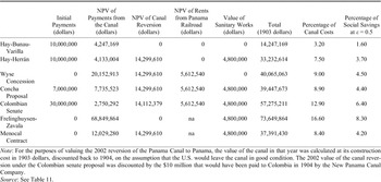
Which counterfactual agreement would have offered the best deal to Panama? Table 13 computes the 1904 net present value of the benefits each would have provided the owner of the Isthmus. The NPV of the (factual) HBV Treaty is less than half the value of a (counterfactual) agreement based on the Hay-Herrán Treaty, to which the United States had in fact agreed and whose terms already incorporated a military threat, and it is barely more than a third of the NPV of agreements based on either the Concha proposal or the Wyse Concession. Even without taking into account the value of the canal's reversion to the owner of the Isthmus, the Hay-Herrán Treaty would have offered benefits worth 33 percent more than what Panama actually received, while an agreement based on the Wyse Concession would have offered 81 percent more, the Concha proposal 77 percent more, and the Senate counteroffer 203 percent more. Contracts based on the two Nicaraguan agreements (also without including the value of the canal reversion) would have offered 62 percent or 122 percent more than Panama in fact received. When the value of the canal's reversion is included, even the least favorable counterfactual agreement (Hay-Herrán) would have provided more than twice as much as the actual HBV Treaty. In terms of the global social savings generated by the canal, the counterfactual agreements would have captured an additional 2.1 to 6.7 percent for the Panamanian government.Footnote 59
NET PRESENT VALUE IN 1904 OF ALTERNATE ISTHMIAN CANAL AGREEMENTS FOR THE PANAMANIAN GOVERNMENT

Note:
For the purposes of valuing the 2002 reversion of the Panama Canal to Panama, the value of the canal in that year was calculated at its construction cost in 1903 dollars, discounted back to 1904, on the assumption that the U.S. would leave the canal in good condition. The 2002 value of the canal reversion under the Colombian senate proposal was discounted by the $10 million that would have been paid to Colombia in 1904 by the New Panama Canal Company.
Source:
See Table 11.
Our calculations likely underestimate the value of the Isthmus under three counterfactual contracts. Under the Wyse Concession, Frelinghuysen-Zavala Treaty, and Menocal Contract, the operator of the canal would have almost certainly charged higher transit rates than the U.S. government actually chose to charge.Footnote 60 In addition, an agreement based on the Menocal Contract (but adapted to Panamanian conditions) would most likely have preserved the rental payment from the Panama Railroad.Footnote 61
CONCLUSION
Does imperialism pay? The American interventions leading to the creation of the Panama Canal certainly did. The canal dramatically cut transportation costs and produced significant savings for world commerce. The lion's share of these savings were captured by the United States because most of the ships passing through the canal carried cargoes coming from or destined for the United States—or in the case of the intercoastal traffic, both—and because the canal produced significant revenues for the U.S. Treasury. Despite cost overruns and long construction delays, the canal was a good investment of public money.
We conclude that the strong-arm tactics that the United States used to build the canal produced substantial dividends for the American economy. From the U.S. point of view, the dividends were at least equal to the difference between the rents Panama stood to gain under a deal comparable to the Wyse Concession versus the actual Hay-Bunau-Varilla Treaty—roughly three percent of the benefits that the world obtained from the canal. (An agreement similar to the one negotiated with Nicaragua in 1884 would have transferred almost seven percent of the canal's social savings to Panama.) In fact, U.S. military prowess and the willingness to use it may have produced even larger gains for the United States; a price discriminating canal operator could have captured far more of the social savings. In this particular case, it appears that not only did imperialism pay, but it seems to have paid quite well.
Appendix: Social Savings Model
We follow Fogel, “Notes,” in defining social savings as the difference between the actual cost of shipping goods in a given year using the Panama Canal versus the cost of shipping the same goods between the same origin and destination in the absence of the Panama Canal. We use a simple two-sector, one-factor model of the world economy, divided into the transportation sector and the remaining sector. In the model, QT represents the output of the transportation sector, QR represents the output of the remaining sector, QTR represents the quantity of QT used in the production of QR, and X represents the production factor used directly in the production of QR and QT. QT can be produced using two technologies: the Panama Canal (pc) or the transcontinental railroad and shipping around the Straits of Magellan (rm). Using the Panama Canal, the same fixed quantity of QT can be produced using less of the production factor X.
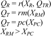
Shutting down the Panama Canal, therefore, would require a transfer of resources from the production of QR to the production of QT in order to maintain a constant level of QT. National income, Y, would then become

where

where

The loss in income (or “social savings”) would then be:

In value terms, then, where PR is the price of a unit of QR, then the “social savings” is equal to

The social savings, S 0, are thus approximately equal to the value of the resources transferred from the transportation sector to the non-transportation when the more efficient technology replaces the less efficient one. The model assumes that the demand for transportation is perfectly inelastic and does not vary with the price. We consider the effects of different elasticities on social savings in the text of the article.