1. Introduction
Reflected processes occupy a prominent role in the literature on operations research and applied probability. In the one-dimensional setting, reflection is specified in terms of the classical Skorokhod problem, and it is widely used to model workload in queues, as well as capital injections and dividends in risk insurance, to name just a few applications. Multidimensional models, allowing for various new features, have been extensively studied as well. We mention only the classical monographs [Reference Cohen and Boxma7] and [Reference Fayolle, Iasnogorodski and Malyshev11], as well as the survey paper [Reference Williams27] on the semimartingale reflected Brownian motion. Apart from some studies of the fundamental properties of the multidimensional model [Reference Lakner, Reed and Zwart21, Reference Taylor and Williams24], most of the work focuses on the recurrent case and the stationary distribution of the reflected process; see [Reference Dieker and Moriarty8, Reference Franceschi and Raschel14] for some recent work. Potential theory and Green functions have also been considered [Reference Bass and Hsu4, Reference Kourkova and Malyshev19]. Another quantity of interest is the probability of hitting the origin for a transient process, which in the insurance context can be interpreted as ruin in a model of two collaborating companies [Reference Albrecher, Azcue and Muler1, Reference Ivanovs and Boxma16]; see also [Reference Hobson and Rogers15, Reference Varadhan and Williams25] for some fundamentals concerning the Brownian model.
In this paper we consider a bivariate Lévy process with a negative mean in a non-standard regime, where the reflection vectors point away from the origin, forcing the reflected process to escape to infinity along one of the axes. We say that the first component totally dominates the second if the process escapes to infinity along the x-axis, that is, the first component grows to infinity while the second becomes relatively negligible; see Figure 1 for an illustration. Under rather general conditions, it is shown in Theorem 3.1 that one of the components dominates the other almost surely and that each component can be dominant with positive probability for any fixed initial position. Additionally, we establish an invariance principle in Theorem 4.1 justifying, for example, the use of the Brownian approximation in applications.
Reflected Brownian motion started at the origin: domination of the first component.

Some of the possible interpretations of our model include the following:
-
Two funds diminishing on average, with an agreement that deficit in one fund is instantaneously covered together with a proportional capital inflow in the other. This inflow may also result indirectly from the loss of rating or trust.
-
Two coupled servers with a special feature that one server, upon becoming idle, hinders the other (or provides some extra work for the other).
We think mainly of the first interpretation and sometimes use the corresponding terminology, such as capital and injections.
It must be noted that the conditions imposed on the reflection angles lead to a non-unique solution of the Skorokhod problem in general, which makes the definition of the model problematic. We resolve this by restricting our attention to certain subclasses of bivariate Lévy processes. Firstly, the model in the Brownian case is defined by [Reference Taylor and Williams24], where the authors also showed its uniqueness in law and derived some important properties. Secondly, a simple iterative construction can be applied if one of the components of the free process does not become negative immediately. In particular, this allows for a compound Poisson process, where each component has a positive linear drift and only negative jumps (cf. the classical Cramér–Lundberg model in risk insurance). We stress that non-uniqueness and the particular implementation of reflection at the origin has no or little effect on our results. Furthermore, we formulate the domination and approximation results in such a way that other models can easily be added upon verification of some basic properties.
Additionally, we identify the Laplace transform of the probability that the first entity wins by totally dominating the second in two important special cases:
-
(i) the aforementioned compound Poisson model with independent components and negative exponential jumps;
-
(ii) the correlated Brownian model.
Firstly, we derive a so-called kernel equation in Case (i), additionally allowing for common jumps (shocks), and then obtain a kernel equation in Case (ii) via approximation, relying on the theory developed below. While in Case (ii) the kernel has already been studied in [Reference Franceschi and Raschel14] for different equations/problems, in Case (i) we have a completely new analytic problem. Even though our kernel equations resemble the one in [Reference Ivanovs and Boxma16], the Wiener–Hopf methods used there seem not to be applicable in the current setting.
The kernel equations are solved by reducing them to the Carleman boundary value problem (BVP) following the general scheme presented in the classical monograph [Reference Fayolle, Iasnogorodski and Malyshev11]. This method, initially proposed in the seventies [Reference Fayolle and Iasnogorodski10, Reference Malyshev22], has been used to study random walks in the quadrant, their invariant measures and Green functions [Reference Kourkova and Raschel18, Reference Kourkova and Malyshev19], and some related queueing models [Reference Baccelli and Fayolle2]. This approach has also been fruitful in the continuous setting for computing the stationary distribution of a reflected Brownian motion in the quadrant [Reference Franceschi and Raschel14]. Our solutions are given in terms of a single contour integral along a half-circle in Case (i) (see Theorem 6.1) and along a half-hyperbola in Case (ii) (see Theorem 7.1). Furthermore, we obtain the probability of domination when starting at the origin and also derive some asymptotic results.
The paper is organized as follows. The model is defined in Section 2, and a basic result concerning the total domination probabilities is proven in Section 3. The approximation result and its proof, relying on the uniform law of large numbers for Lévy processes, are given in Section 4. The kernel equations for the models (i) and (ii) are derived in Section 5 from the one for the Poissonian model with common shocks. With regard to the latter equation, we only summarize the basic steps; the corresponding lengthy and tedious calculations are presented in Appendix A. We solve the kernel equation for the Poissonian model (i) in Section 6 and for the Brownian model (ii) in Section 7. Finally, numerical illustrations are provided in Section 8.
2. Definition of the model
Consider a probability space with filtration
 ${\mathcal{F}}_t$
, and let
 $X(t)=(X_1(t),X_2(t))$
,
 $t \geqslant 0$
, be an adapted bivariate Lévy process, that is, a process with stationary and independent increments which is continuous in probability; without loss of generality, we assume that it has càdlàg paths without fixed jumps (e.g., see [Reference Kallenberg17, Theorem 15.1]). Our main examples will be a correlated Brownian motion and a drifted compound Poisson process, whose two components may exhibit both individual and common jumps.
2.1. Skorokhod problem
A bivariate process
 $Y \geqslant 0$
is a solution to the Skorokhod problem [Reference Williams27], also known as the dynamic complementarity problem, if the following holds almost surely (a.s.):
 \begin{equation}\begin{split}Y_1(t)=u+X_1(t)+L_1(t)+r_2L_2(t),\\Y_2(t)=v+X_2(t)+r_1L_1(t)+L_2(t),\end{split}\end{equation}
where (u,v) is the starting position with
 $u,v \geqslant 0$
, and the
 $L_i$
are the regulators (cumulative capital injections) satisfying
-
(i)
 $L_i(t)$
is non-decreasing with
$L_i(0)=0$
;
-
(ii)
$L_i(t)$
increases only when
$Y_i(t)=0$
, i.e.,
$\int_0^\infty Y_i(s){\mathrm{d}} L_i(s)=0$
.


It is assumed that all the processes are adapted to the given filtration. The second condition concerns minimality of injections, meaning that no injections are received unless strictly necessary; in particular, we have
 \begin{equation*}\begin{gathered}L_1(t)=\sup_{0 \leqslant s \leqslant t} \left[{-}u-X_1(s)-r_2L_2(s)\right]\vee 0,\\L_2(t)=\sup_{0 \leqslant s \leqslant t} \left[{-}v-X_2(s)-r_1L_1(s)\right]\vee 0.\end{gathered}\end{equation*}
In contrast to the classical setting, we assume that
 \begin{equation}r_1,r_2>0\qquad \text{ and }\qquad r_1r_2>1.\end{equation}
The corresponding reflection matrix
 $\left(\begin{smallmatrix} 1 & r_2\\ r_1 & 1\end{smallmatrix}\right)$
belongs to the so-called completely-
 ${\mathcal{S}}$
class and thus our Skorokhod problem has a solution in the sample-path sense [Reference Kozyakin, Mandelbaum and Vladimirov20]. Uniqueness, however, is not guaranteed, leading to certain measurability issues for general processes; see [Reference Bernard and El Kharroubi5, Reference Williams27]. Nevertheless, in the Brownian case there is a unique weak solution [Reference Taylor and Williams24]. Moreover, [Reference Williams28] establishes an invariance property allowing one to retrieve the Brownian model as a weak limit of approximations on compact time intervals.
2.2. Iterative definition and linear complementarity problem
To define the reflected process for a more general X, we need to recall an important dichotomy for one-dimensional Lévy processes: the probability of immediate entrance into the negative half-line
 $({-}\infty,0)$
is either 0 or 1. In the first case the entrance time is strictly positive and the main example is a process of bounded variation on compacts with a positive linear drift [Reference Bertoin6, Proposition VI.11].
Coming back to the bivariate process X, we assume that at least one of its components enters
 $({-}\infty,0)$
at a strictly positive time. Without loss of generality, we assume that
 $X_2$
is such, and let
 $T_k$
,
 $k \geqslant 1$
, be the random times when
 $X_2$
(or, equivalently,
 $v+X_2$
) updates its infimum; for convenience, we also set
 $T_0=0$
. It is clear that if
 \begin{align*}v+X_2(T_{k-1})+r_1L_1(T_{k-1})+L_2(T_{k-1}) \geqslant 0,\end{align*}
then, since
 $r_1>0$
, we also have
 \begin{align*}v+X_2(t)+r_1L_1(t)+L_2(T_{k-1}) \geqslant 0,\quad T_{k-1} \leqslant t<T_k;\end{align*}
besides,
 $T_k\to\infty$
a.s. as
 $k\to\infty$
. Therefore, in order to obtain the reflected process Y on
 $[0,+\infty)$
, we just need to define it on the intervals
 $[T_{k-1},T_k)$
,
 $k \geqslant 1$
, keeping
 $L_2$
constant on them.
To this end, we set
 $L_2(t)=0$
for
 $t<T_1$
, and then define Y on
 $[0,T_1)$
by reflecting
 $u+X_1+r_2L_2$
in the one-dimensional sense up to
 $T_1$
, i.e. taking
 \begin{align*}L_1(t)=-\inf_{0 \leqslant s \leqslant t} [0\wedge (u+X_1(s))],\quad t<T_1.\end{align*}
Then, loosely speaking, at the moment
 $T_1$
we solve the corresponding linear complementarity problem, reset Y accordingly, and proceed from there, repeating the procedure. More precisely, at each epoch
 $T_k$
, which is a stopping time, we let
 \begin{align*}x_i=Y_i(T_k-)+\Delta X_i(T_k),\quad i=1,2,\end{align*}
where
 $\Delta X_i(T_k)=X_i(T_k)-X_i(T_k-)$
, and solve the linear complementarity problem for this
 $x=(x_1,x_2)\in{\mathbb{R}}^2$
:
 \begin{equation}y_1=x_1+\ell_1+r_2\ell_2,\qquad y_2=x_2+\ell_2+r_1\ell_1,\end{equation}
where
 $y_i,\ell_i \geqslant 0$
and
 $\ell_iy_i=0$
. Then we set
 $Y_i(T_k)=y_i$
,
 $L_i(T_k)=L_i(T_k-)+\ell_i$
, and proceed as if
 $Y(T_k)=(y_1,y_2)$
were the starting position instead of (u,v) and
 $X(T_k+\cdot)-X(T_k)$
were the free process instead of X, whereas we let L accumulate the needed future injections.
Thus defined, the processes Y,
 $L_1$
, and
 $L_2$
are clearly adapted to the given filtration and satisfy (2.1) together with (i) and (ii). In addition, if both
 $X_1$
and
 $X_2$
enter
 $({-}\infty,0)$
at a strictly positive time, then
 $L_1$
and
 $L_2$
are piecewise constant and do not depend on the initial choice of the component of X for which the
 $T_k$
are constructed.
However, it turns out that the static problem (2.3) can have multiple solutions for certain
 $(x_1,x_2)<0$
. In principle, any of these can be used, and one may even pick a solution in an
 ${\mathcal{F}}_{T_k}$
-measurable random way. However, we choose one specific solution, which we are now going to describe.
In the static problem (2.3),
 $x_i \geqslant 0$
necessarily implies that
 $\ell_i=0$
. In particular,
 $x_1,x_2 \geqslant 0$
yields
 $y_i=x_i$
(no adjustment). Furthermore, if
 $x_1<r_2x_2\wedge 0$
, then
 $y_1=0$
and
 $y_2=x_2-r_1x_1$
, whereas if
 $x_2<r_1x_1\wedge 0$
, then
 $y_1=x_1-r_2x_2$
and
 $y_2=0$
. The final case concerns the wedge:
 \begin{align*}x_1,x_2<0,\quad x_1 \geqslant r_2x_2,\quad x_2 \geqslant r_1x_1;\end{align*}
see also Figure 2. Here we have three solutions (two on the boundary):
-
(i)
$y_1=y_2=0$
, -
(ii)
$y_1=x_1-r_2x_2,\quad y_2=0$
, -
(iii)
$y_1=0,\quad y_2=x_2-r_1x_1$
.


Solutions to the linear complementarity problem (2.3). The blue half-line corresponds to
 $x_1=r_2x_2<0$
and the red to
 $x_2=r_1x_1<0$
. The red region results in
 $y_1=0$
and the blue region in
 $y_2=0$
. The wedge corresponds to three solutions, and for concreteness we choose
 $y_1=y_2=0$
there.

In the following we pick (i) for concreteness, which resets both components to 0 when ambiguity arises. It is noted that this particular choice has no or little effect on our results, which we also stress in the following.
Finally, it is worth mentioning that in a similar way one can construct the reflected process for the sum of a Brownian motion and an arbitrary independent compound Poisson process, where between the jumps the model evolves as a reflected Brownian motion and at jump epochs we again solve (2.3).
2.3. Basic properties
Here we observe some basic properties of the reflected process. Firstly, note that the regulator does not increase when the free process is non-negative:
 \begin{equation}\forall\, t\in [0,T]\,:\,\quad u+X_1(t) \geqslant 0\qquad \Longrightarrow\qquad L_1(T)=0,\end{equation}
since from (2.1) we then have
 $Y_1(t) \geqslant L_1(t)$
and thus
 $\int_0^T L_1(t){\mathrm{d}} L_1(t)=0$
. In such a case
 $L_2(t)=({-}\inf_{0 \leqslant s \leqslant t} [v+X_2(s)])^+$
and the expressions for
 $Y_1$
and
 $Y_2$
are straightforward. Unlike in the classical case, however, non-uniqueness presents some problems: if
 $L_1(T)=0$
yields a non-negative solution (and even
 $Y_1$
may be strictly positive on [0,T]), then we cannot conclude that this is the right solution.
Importantly,
 \begin{equation}\text{$Y$ is strong Markov},\end{equation}
so that for any finite stopping time
 $\tau$
, conditional on
 $Y(\tau)=(u^{\prime},v^{\prime})$
, the process
 $Y^{\prime}(t)=Y(\tau+t)$
is independent of
 ${\mathcal{F}}_\tau$
and has the original law when started at
 $(u^{\prime},v^{\prime})$
. In the Brownian case this is a consequence of the strong Feller property shown in [Reference Taylor and Williams24], and in the case of the iterative construction of Section 2.2 this property is obviously inherited from the process X. Note, however, that the choice in (2.3) must not depend on the future evolution of the process.
Finally we comment on rescaling of the model. For any
 $a_1,a_2>0$
, by setting
 \begin{equation}X^{\prime}_i(t)=a_iX_i(t),\quad u^{\prime}=a_1u,\quad v^{\prime}=a_2 v,\quad r^{\prime}_1=\dfrac{a_2}{a_1}r_1,\quad r^{\prime}_2=\dfrac{a_1}{a_2}r_2,\end{equation}
we find that
 $Y^{\prime}_i(t)=a_iY_i(t)$
, with
 $L^{\prime}_i(t)=a_iL_i(t)$
being a solution of (2.1). Furthermore, we resolve non-uniqueness in Section 2.2 in a consistent way, implying
 $Y^{\prime}_i(t)=a_i Y_i(t)$
. Thus, the probability of total domination defined in Section 3 is invariant under any such scaling given that the initial position is scaled appropriately.
Reflection vectors and the mean.

3. Domination
3.1. The result
We assume throughout this paper that X is a bivariate Lévy process (with càdlàg paths) such that
 \begin{align}\tag{A1}{\mathbb{E}} X(1)=\mu=(\mu_1,\mu_2)<0,\end{align}
 \begin{align}\tag{A2}r_1{\lvert}\mu_1{\rvert}>{\lvert}\mu_2{\rvert},\qquad r_2{\lvert}\mu_2{\rvert}>{\lvert}\mu_1{\rvert},\end{align}
where the latter implies (2.2). Furthermore, we assume that the reflected process Y is well-defined in the sense that it satisfies (2.1) and (2.5). It is noted that in the Brownian case the above conditions imply that Y is transient [Reference Hobson and Rogers15], but more is true, as we show in the following.
An additional technical assumption is needed to exclude certain degenerate cases:
 \begin{equation}\tag{A3}{\mathbb{P}}\big\{\exists\, t>0\,:\, X_i(t)>0,\; X_j(t)={\underline{X}}_j(t)\big\}>0,\quad (i,j)=(1,2),\; (2,1),\end{equation}
where
 ${\underline{X}}_j(t)\,:\!=\,\inf_{0 \leqslant s \leqslant t} X_j(s)$
. This condition is not minimal possible, but we avoid further technicalities since it is broadly satisfied. Importantly, for the Brownian model it is sufficient to assume that its correlation
 $\rho$
is not 1. For the compound Poisson model with positive linear drift c it is sufficient to assume that both components may exhibit individual negative jumps. As an example not satisfying (A3), consider jumps distributed as
 $(\Delta_1,\Delta_2)$
, where
 $\Delta_i<0$
and
 ${\mathbb{P}}(\Delta_1/\Delta_2 \geqslant c_1/c_2)$
is either 1 or 0. It should be mentioned that such models with ordered jumps have been used, for example, in [Reference Badila, Boxma, Resing and Winands3], because they allow for simpler analysis in various settings.
Our focus is on the probabilities
 $p_i=p_i(u,v)$
of total domination starting from (u,v), which are defined by
 \begin{gather*}p_1(u,v)={\mathbb{P}}_{(u,v)}\left\lbrace Y_1(t)\to\infty,\; \dfrac{Y_2(t)}{Y_1(t)}\to 0\right\rbrace,\\[6pt]p_2(u,v)={\mathbb{P}}_{(u,v)}\left\lbrace Y_2(t)\to\infty,\; \dfrac{Y_1(t)}{Y_2(t)}\to 0\right\rbrace.\end{gather*}
The following result shows that total domination is certain, and each component can be the dominant one for any starting position.
Theorem 3.1 (Total domination probabilities). Under the conditions (A1), (A2), and (A3) for any
 $(u,v)\in{\mathbb{R}}^2_+$
we have the following:
 \begin{align*}p_1(u,v)\in (0,1)\qquad and \qquad p_1(u,v)+p_2(u,v)=1.\end{align*}
Moreover,
 $\lim\limits_{u\to\infty} p_1(u,v)=1$
and
 $\lim\limits_{v\to\infty} p_1(u,v)=0$
.
The proof of this result is based on two lemmas and the observation that Y visits the boundary infinitely often. Firstly, we employ a regeneration argument to show that Y hits the remote parts of the quadrant boundary a.s. Secondly, when starting in those remote parts, the process Y has the claimed behaviour with high probability, which follows from the strong law of large numbers and some basic properties underlying (2.1).
3.2. Proofs
By the law of large numbers, we have
 \begin{equation}\dfrac{X_i(t)}{t}{\xrightarrow{\mathrm{a.s.}}}\mu_i,\quad t\to\infty,\quad i=1,2;\end{equation}
see, e.g., [Reference Sato23, Theorem 36.5]. This implies that if the conditions (A1) and (A2) are satisfied, then the reflected stochastic process Y hits the boundary
 $\partial{\mathbb{R}}_+^2$
infinitely often:
 \begin{align*}\sup\{t \geqslant 0\,:\, Y_1(t)\wedge Y_2(t)=0\}=\infty\quad {\mathrm{a.s.}}\end{align*}
Indeed, suppose that
 $\tau=\sup\{t \geqslant 0\,:\, Y_1(t)=0\}<\infty$
. By definition, we have
 $Y_1(t)>0$
,
 $t>\tau$
, and so
 $L_1(t)=L_1(t\wedge\tau)$
,
 $t \geqslant 0$
. Therefore, using (3.1), we obtain
 \begin{align*}\lim_{t\to\infty} \dfrac{L_2(t)}{t}=\lim_{t\to\infty} \dfrac{1}{t}\sup_{0 \leqslant s \leqslant t} ({-}v-X_2(s)-r_1L_1(s\wedge\tau))^+=-\mu_2>0\quad {\mathrm{a.s.}},\end{align*}
which implies that
 $\sup\{t \geqslant 0\,:\, Y_2(t)=0\}=\infty$
.
However, if the condition (A3) is also fulfilled, then a stronger assertion holds true; namely, the reflected process hits the remote parts of the boundary
 $\partial{\mathbb{R}}_+^2$
a.s.
Lemma 3.1. Assume the conditions (A1), (A2), and (A3), and for any
 $h>0$
define two disjoint sets
 \begin{align*}D^1_h=\{(x,0)\,:\, x \geqslant h\},\qquad D^2_h=\{(0,y)\,:\, y \geqslant h\}.\end{align*}
Then, for any fixed
 $(u,v)\in{\mathbb{R}}_+^2$
and all
 $h>0$
, the stochastic process Y satisfies the following:
 \begin{align*}&{\mathbb{P}}_{(u,v)}\left\lbrace\exists\, t \geqslant 0\,:\, Y(t)\in D_h^1\cup D_h^2\right\rbrace=1,\\&{\mathbb{P}}_{(u,v)}\,\Big\lbrace\exists\, t \geqslant 0\,:\, Y(t)\in D_h^i\Big\rbrace>0,\quad i=1,2.\end{align*}
Proof. Note that the law of large numbers (3.1) and the condition (A3) imply that the paths of
 $X_1$
and
 $X_2$
take both positive and negative values, and so are not monotone functions with probability one. In addition, by the condition (A3) we have
 \begin{align*}{\mathbb{P}}\left\lbrace\exists\, t>0\,:\, X_1(t)>0,\; X_2(t)={\underline{X}}_2(t)\right\rbrace>0.\end{align*}
Furthermore, since
 $\mu_2<0$
, we can add
 ${\underline{X}}_2(t)<0$
into this probability to get
 \begin{equation}{\mathbb{P}}\left\lbrace\exists\, t>0\,:\, X_1(t)>0,\; X_2(t)={\underline{X}}_2(t)<0\right\rbrace>0.\end{equation}
Fixing any
 $\delta>0$
, we note that since
 $X_1$
is not non-increasing it can become arbitrarily large before becoming
 $ \leqslant -\delta$
. Thus, using the strong Markov property and applying (3.2) sufficiently many times, we obtain
 \begin{align*}{\mathbb{P}}\left\lbrace\exists\, t>0\,:\, X_1(t)>1,\; {\underline{X}}_1(t)>-\delta,\; X_2(t)= {\underline{X}}_2(t)<0\right\rbrace>0,\end{align*}
and hence for some
 $T>0$
 \begin{equation}c={\mathbb{P}}\left\lbrace\exists\, t\in (0,T]\,:\, X_1(t)>1,\; {\underline{X}}_1(t)>-\delta,\; X_2(t)= {\underline{X}}_2(t)<0\right\rbrace>0.\end{equation}
As was shown at the beginning of this subsection, the stochastic process Y visits the boundary of
 ${\mathbb{R}}_+^2$
infinitely often. Assume that for some
 $\delta>0$
the process Y visits
 $D_\delta^1\cup D_\delta^2$
infinitely often. Let us show, using a regeneration argument, that the same is then true for
 $\delta^{\prime}=\delta+1$
. Consider an increasing sequence of stopping times
 $\tau_1,\tau_2,\ldots$
defined as the successive visits of the set
 $D_\delta^1$
with at least T time units in between:
 \begin{align*}\tau_1 & =\inf\big\{t \geqslant 0\mid Y(t)\in D_\delta^1\big\},\\[4pt]\tau_{i+1}= & \inf\big\{t \geqslant \tau_i+T\mid Y(t)\in D_\delta^1\big\},\quad i \geqslant 1.\end{align*}
For each i such that
 $\tau_i<\infty$
, let
 $u_i=Y_1(\tau_i)$
, and consider the probability that Y hits
 $D^1_{u_i+1}$
in
 $[\tau_i,\tau_i+T]$
, but before
 $Y_1$
becomes less than or equal to
 $u_i-\delta$
, which will mean that it hits
 $D^1_{\delta+1}$
. This probability is constant for all i and is given by (3.3). Hence, the probability of not visiting
 $D^1_{\delta+1}$
is bounded above by
 $(1-c)^{N_1}$
, where
 $N_1$
is the number of
 $\tau_i<\infty$
. The same is true for the other direction. Since at least one of
 $N_1,N_2$
is infinite, this implies that visiting
 $D^1_{\delta+1}\cup D^2_{\delta+1}$
is certain.
Also, we note that if only the origin is visited infinitely often, then we may apply a similar regeneration argument at the origin to get a contradiction. Therefore, the above argument proves the first claim.
To prove the second statement, we note that the probability of hitting the boundary at a point other than the origin is positive. Firstly,
 $Y_1$
must be positive, since
 $X_1$
is not non-increasing. But for a positive u we may again apply (3.3), showing that hitting the ray (x, 0),
 $x>0$
, is possible. This also shows that hitting
 $D^1_h$
for any
 $h>0$
and any starting position (u, v) occurs with positive probability. A similar argument holds for the other component, which completes the proof.
The following lemma shows that if the initial capital of one of the companies is sufficiently large, then this company will dominate with probability close to one. Its proof is based on the law of large numbers (3.1) for Lévy processes.
Lemma 3.2. If the conditions (A1) and (A2) are satisfied, then for any
 ${\varepsilon}>0$
there exists
 $u_0=u_0({\varepsilon}) \geqslant 0$
such that
 \begin{align*}p_1(u,v) \geqslant 1-{\varepsilon}\end{align*}
for all
 $v \geqslant 0$
and
 $u \geqslant (r_2v)\vee u_0$
. Also, a similar assertion holds true for
 $p_2$
.
Proof. We note that (3.1) implies
 \begin{align*}\sup_{t \geqslant T} \dfrac{X_i(t)}{t}{\xrightarrow{\mathbb{P}}}\mu_i,\quad T\to\infty,\quad i=1,2.\end{align*}
Therefore, fixing arbitrarily small
 ${\varepsilon}>0$
(more precisely, we will later need that
 ${\varepsilon}<{\varepsilon}_0$
, where
 ${\varepsilon}_0=(r_2{\lvert}\mu_2{\rvert}-{\lvert}\mu_1{\rvert})/(2r_2+2)>0$
), we can choose
 $T=T({\varepsilon})>0$
such that
 \begin{align*}{\mathbb{P}}\left\lbrace\sup_{t \geqslant T} \max_{i=1,2} \left\lvert\dfrac{X_i(t)}{t}-\mu_i \right\rvert < {\varepsilon}\right\rbrace= {\mathbb{P}}\left\lbrace\max_{i=1,2} \sup_{t \geqslant T} \left\lvert\dfrac{X_i(t)}{t}-\mu_i \right\rvert <{\varepsilon}\right\rbrace \geqslant 1-\dfrac{{\varepsilon}}{2}.\end{align*}
Then we have
 \begin{equation}(\mu_i-{\varepsilon})t<X_i(t)<(\mu_i+{\varepsilon})t,\quad t \geqslant T,\quad i=1,2,\end{equation}
with probability not less than
 $1-{\varepsilon}/2$
. Also, let
 $u_0>0$
be so large that
 \begin{align*}{\mathbb{P}}\left\lbrace{-}{\underline{X}}_1(T)<u_0\right\rbrace \geqslant 1-{\varepsilon}/2.\end{align*}
In the rest of the proof we focus on the intersection of these two events, which has probability not less than
 $1-{\varepsilon}$
.
Now, fix arbitrary
 $v \geqslant 0$
and
 $u \geqslant (r_2v)\vee u_0$
, consider the random time
 \begin{align*}\tau=\inf\{t \geqslant 0 \mid L_1(t)>0\} \geqslant T,\end{align*}
and let us show that actually
 $\tau=\infty$
. Indeed, we first note that if
 $\tau=T$
, then
 $L_1(\tau)=0$
, because
 \begin{align*}Y_1(\tau)=Y_1(T) \geqslant u+X_1(T) \geqslant u_0-\big({-}{\underline{X}}_1(T)\big)>0.\end{align*}
Moreover, if
 $\tau>T$
, then, by the definition of
 $\tau$
, for any
 $T \leqslant t<\tau$
we have
 $L_1(t)=0$
, and using (3.4) we obtain
 \begin{align}L_2(t) & \geqslant \sup_{0 \leqslant s \leqslant t} ({-}v-X_2(s)-r_1L_1(s))^+=\sup_{0 \leqslant s \leqslant t} \big({-}v-X_2(s)\big)^+\nonumber\\& \geqslant \sup_{T \leqslant s \leqslant t} \big({-}v-X_2(s)\big)^+ \geqslant ({\lvert}\mu_2{\rvert}-{\varepsilon})t-v.\end{align}
Hence, for such t we have
 \begin{align*}Y_1(t) \geqslant u+X_1(t)+r_2L_2(t) \geqslant u-({\lvert}\mu_1{\rvert}+{\varepsilon})t+r_2({\lvert}\mu_2{\rvert}-{\varepsilon})t-r_2v \geqslant (u-r_2v)+ct>0,\end{align*}
where
 $c=(r_2{\lvert}\mu_2{\rvert}-{\lvert}\mu_1{\rvert})/2>0$
. Furthermore, the fact that
 $X_1(\tau) \geqslant -({\lvert}\mu_1{\rvert}+{\varepsilon})\tau$
and
 $L_2$
is monotone implies that this bound also holds true for
 $t=\tau$
.
Therefore, in both cases we have
 $Y_1(\tau)>0$
. Owing to the right continuity of
 $X_1$
and monotonicity of
 $L_1$
and
 $L_2$
, we have
 $Y_1(t)>0$
for any
 $t\in (\tau,\tau+\delta)$
with sufficiently small
 $\delta>0$
. This means that
 $L_1(t)=0$
for
 $t\in (\tau,\tau+\delta)$
, which contradicts the definition of
 $\tau$
.
Thus, we conclude that for
 $u \geqslant (r_2v)\vee u_0$
the stochastic process
 $Y_1$
stays positive at all times. So for all
 $t \geqslant 0$
we have
 \begin{align*}Y_1(t) & = u+X_1(t)+r_2L_2(t),\qquad Y_2(t)=v+X_2(t)+L_2(t),\\L_2(t) & =\sup_{0 \leqslant s \leqslant t} \big({-}v-X_2(s)\big)^+.\end{align*}
It is easy to check that
 \begin{align*}\lim_{t\to\infty} \dfrac{L_2(t)}{t}={\lvert}\mu_2{\rvert},\qquad \lim_{t\to\infty} \dfrac{Y_1(t)}{t}= r_2{\lvert}\mu_2{\rvert}-{\lvert}\mu_1{\rvert}>0,\qquad \lim_{t\to\infty} \dfrac{Y_2(t)}{t}=0.\end{align*}
Hence, the event of interest is ensured with probability not less than
 $1-{\varepsilon}$
.
The same argument is valid for the corresponding assertion with
 $p_2$
.
Proof of Theorem 3.1. Fix arbitrary
 $u,v \geqslant 0$
. For any
 ${\varepsilon}>0$
choose
 $u_0=u_0({\varepsilon})>0$
and
 $v_0=v_0({\varepsilon})>0$
as in Lemma 3.2, set
 $h=u_0\vee v_0$
, and consider
 \begin{align*}\tau_1=\inf\left\lbrace t \geqslant 0\,:\, Y(t)\in D^1_h\right\rbrace,\qquad \tau_2=\inf\left\lbrace t \geqslant 0\,:\, Y(t)\in D^2_h\right\rbrace,\end{align*}
which are stopping times with respect to the given filtration.
By Lemma 3.1 the event
 $\{\tau_1<\infty\}$
has positive probability, and on this event the shifted process
 $X^{\prime}(t)=X(\tau_1+t)-X(\tau_1)$
has the same law as the original Lévy process and is independent of the corresponding position
 $Y(\tau_1)\in D^1_{u_0}$
(see [Reference Bertoin6, Proposition I.6]). Therefore, noting that
 \begin{align*}p_1(u,v)={\mathbb{P}}_{(u,v)}\left\lbrace\tau_1<\infty,\; Y_1(t)\to\infty,\; \dfrac{Y_2(t)}{Y_1(t)}\to 0\right\rbrace,\end{align*}
we obtain, by Lemma 3.2,
 \begin{align*}p_1(u,v) & ={\mathbb{E}}_{(u,v)}\left[{1\negmedspace\mathrm{I}}\{\tau_1<\infty\}\cdot{\mathbb{P}}_{Y(\tau_1)}\left\lbrace Y_1(t)\to\infty,\; \dfrac{Y_2(t)}{Y_1(t)}\to 0\right\rbrace\right]\\& \geqslant (1-{\varepsilon})\cdot{\mathbb{P}}_{(u,v)}\{\tau_1<\infty\},\end{align*}
and so
 \begin{equation}(1-{\varepsilon})\cdot{\mathbb{P}}_{(u,v)}\{\tau_1<\infty\} \leqslant p_1(u,v) \leqslant {\mathbb{P}}_{(u,v)}\{\tau_1<\infty\}.\end{equation}
Similar bounds hold true for
 $p_2(u,v)$
and
 $\tau_2$
. Hence, according to Lemma 3.1, both
 $p_1$
and
 $p_2$
are positive, which proves the first assertion, and also
 $p_1+p_2 \geqslant 1-{\varepsilon}$
, which, by the arbitrariness of
 ${\varepsilon}$
, implies the second assertion.
4. Approximation
4.1. Assumptions
Throughout this section we consider a sequence of bivariate Lévy processes
 $X^{(n)}$
converging weakly to X with respect to the Skorokhod
 $J_1$
-topology [Reference Whitt26, Section 3.3]. This is equivalent to
 \begin{equation}\tag{C1}X^{(n)}(1){\xrightarrow{\mathrm{d}}} X(1),\end{equation}
or to the convergence of the Lévy exponents [Reference Kallenberg17, Theorem 15.17]. Furthermore, we assume that the means also converge:
 \begin{equation}\tag{C2}\mu^{(n)}={\mathbb{E}} X^{(n)}(1)\to{\mathbb{E}} X(1)=\mu,\end{equation}
which is equivalent, in view of (C1), to the uniform integrability of
 $X^{(n)}(1)$
.
It is assumed that the reflected processes Y and
 $Y^{(n)}$
are well-defined, so that they satisfy (2.1) and (2.5). Now we may expect that
 \begin{equation}\tag{C3}Y^{(n)}{\xrightarrow{\mathrm{d}}} Y\qquad \text{whenever}\quad {\mathbb{R}}_+^2\ni \big(u^{(n)},v^{(n)}\big)\to (u,v),\end{equation}
which is indeed broadly satisfied for our models, including the case when Y is a reflected Brownian motion, as shown by [Reference Williams28]. Nevertheless, some exceptions exist, as we now describe. The degenerate case is given by a drifted compound Poisson process with linear drifts
 $c_i>0$
and jumps distributed as
 $(J_1,J_2)$
, where
 \begin{equation}c_i=r_jc_j\text{ and }J_i-r_jJ_j\text{ has a point mass}\end{equation}
for some
 $i\in\{1,2\}$
and
 $j\neq i$
.
Lemma 4.1 (Convergence of reflected processes). The convergence in (C1) implies (C3) in the following cases:

Proof. The first statement is a consequence of [Reference Williams28, Theorem 4.1 and Proposition 4.2(III)], where uniform integrability and the martingale property readily follow from (C2).
Next, we consider the iterative construction of the reflected process, and recall that the one-dimensional reflection is a continuous map [Reference Whitt26, Section 13.5]. It is important that we resolve non-uniqueness of (2.3) in the same way for all processes; recall that we have chosen to restart the processes from the origin if ambiguity arises. Our reflection map is then continuous at sample paths requiring finitely many iterations and not hitting the boundary of the wedge right before the application of linear complementarity; see Figure 2. It is thus sufficient to show that the boundary of the wedge is not hit at the time
 $T_1$
in the construction of the limit process Y with probability 1.
Suppose that this occurs with positive probability. Since the jumps of X below some negative threshold are independent, we see that
 $Y(T_1-)$
must have a mass on some line parallel to one of the wedge boundaries. Furthermore, we may replace
 $T_1$
by an independent exponential time. Assume for a moment that X is not compound Poisson, in which case the distribution of
 $X_t$
for any
 $t>0$
is continuous [Reference Sato23, Theorem 27.4]. Ignoring the reflection we easily derive a contradiction by taking t small and projecting X onto the perpendicular direction. This argument can be extended to the case when
 $X_1$
does not spend time at the boundary (the Lebesgue measure is 0). In the only other case we may look at
 $X_2-r_1X_1$
to get the contradiction. Finally, assume that X is a compound Poisson. The only possibility here is that included into (4.1).
4.2. The result and its proof
Let us now state the approximation result for the domination probabilities. In fact, we show continuous convergence in the sense that perturbations in the initial positions are also allowed. Importantly, (C3) is equivalent to convergence of the reflected process on compact intervals of time, and thus convergence of the limiting quantities is not obvious.
Theorem 4.1 (Invariance principle). Assume that X satisfies the conditions of Theorem 3.1, and let
 $X^{(n)}$
be a sequence of bivariate Lévy processes approximating X so that (C1), (C2), and (C3) hold. Then
 \begin{align*}\lim_{n\to\infty} p_i^{(n)}\big(u^{(n)},v^{(n)}\big)=p_i(u,v),\qquad i=1,2,\end{align*}
whenever
 ${\mathbb{R}}_+^2\ni\big(u^{(n)},v^{(n)}\big)\to (u,v)$
. In particular, the
 $p_i$
are continuous for such X.
The main ingredient of the proof is the following uniform law of large numbers for Lévy processes.
Lemma 4.2. Let
 $X,X^{(n)}$
be bivariate Lévy processes satisfying (C1) and (C2). Then
 \begin{equation}\lim_{T\to\infty} \limsup_{n\to\infty} {\mathbb{P}}\left\lbrace\sup_{t \geqslant T} \max_{i=1,2} {\lvert}\dfrac{X_i^{(n){\rvert}(t)}{t}-\mu_i}>{\varepsilon}\right\rbrace=0\end{equation}
for any
 ${\varepsilon}>0$
.
Proof. Without loss of generality, we consider the one-dimensional case and assume that
 $\mu=0$
. Let us show that the stochastic process
 $\{M_{-t}=X(t)/t,\; t>0\}$
is a martingale with respect to the filtration
 ${\mathcal{G}}_{-t}=\sigma\left\lbrace X(t+s),\; s \geqslant 0\right\rbrace$
, i.e., that for any
 $t>0$
and
 $s \geqslant 0$
,
 \begin{equation}{\mathbb{E}}\left[\left.\dfrac{X(t)}{t}\right| X(t+s)\right]=\dfrac{X(t+s)}{t+s}.\end{equation}
By the right continuity of the sample paths, it is sufficient to take
 $t=m(t+s)/n$
for some integers
 $m \leqslant n$
. However, it is a standard fact that for independent and identically distributed
 $Z_i$
with finite first moment we have the identity
 \begin{align*}{\mathbb{E}}[Z_1+\cdots+Z_m \mid Z_1+\cdots+Z_n]=\dfrac{m}{n}(Z_1+\cdots+Z_n),\end{align*}
and taking
 $Z_i=X(i(t+s)/n)-X((i-1)(t+s)/n)$
we get (4.3).
Now, by Doob’s martingale inequality [Reference Kallenberg17, Proposition 7.15], for any
 $T^{\prime}>T$
we have
 \begin{equation}{\mathbb{P}}\left\lbrace\sup_{t\in [T,T^{\prime}]} \dfrac{{\lvert}X(t){\rvert}}{t} \geqslant {\varepsilon}\right\rbrace \leqslant \dfrac{1}{{\varepsilon}}\cdot\dfrac{{\mathbb{E}}{\lvert}X(T){\rvert}}{T},\end{equation}
which, by passing to the limit, readily extends to the infinite time interval
 $[T,\infty)$
.
Thus, to prove (4.2), it is sufficient to show that
 \begin{align*}\lim_{T\to\infty} \limsup_{n\to\infty} \dfrac{{\mathbb{E}}{\lvert}X^{(n){\rvert}(T)}}{T}=0.\end{align*}
However, for a fixed T we have
 $X^{(n)}(T){\xrightarrow{\mathrm{d}}} X(T)$
as
 $n\to\infty$
, which implies the convergence of the mean absolute values, because the families
 $X^{(n)}(1)$
,
 $n \geqslant 1$
, and thus also
 $X^{(n)}(T)$
,
 $n \geqslant 1$
, are uniformly integrable. Finally, from (4.4) with the infinite time interval
 $[T,\infty)$
, it is easy to deduce that the family
 ${\lvert}X(t){\rvert}/t$
,
 $t \geqslant T$
, is uniformly integrable, and so
 ${\mathbb{E}}{\lvert}X(T){\rvert}/T\to 0$
as
 $T\to\infty$
(see also [Reference Sato23, Theorem 36.5]).
Proof of Theorem 4.1. Fix
 ${\varepsilon}>0$
and note that the bounds in (3.6) hold for all large n, since then the conditions (A1) and (A2) are satisfied. Note, however, that
 $u_0$
there depends on n. Nevertheless, we can choose
 $u_0^{(n)}=u_0$
independently of n; see the proof of Lemma 3.2. This is so because we may use the same T according to Lemma 4.2, but then
 $\underline X_1^{(n)}(T){\xrightarrow{\mathrm{d}}} \underline X_1(T)$
. Furthermore, the bounds in Lemma 3.2 are also true if the set
 $D^{\prime}_{u_0}=\{(u,v)\in{\mathbb{R}}_+^2\,:\, u \geqslant (r_2v)\vee u_0\}$
is replaced by
 $D_{u_0+\delta}^1$
for any
 $\delta>0$
as defined in Lemma 3.1.
Let
 $p_1(T)$
be the probability that Y hits
 $D_{u_0+1}^1$
on [0,T] starting from (u,v), and let
 $p_1^{(n)}(T)$
be the probability that
 $Y^{(n)}$
hits
 $D^{\prime}_{u_0}$
on [0,T] starting from
 $\big(u^{(n)},v^{(n)}\big)$
. We choose
 $T \geqslant 0$
so large that
 \begin{align*}0 \leqslant {\mathbb{P}}_{(u,v)}\big\{\text{$Y$ hits $D_{u_0+1}^1$}\big\}-p_1(T)<{\varepsilon}.\end{align*}
Then, by (3.6),
 \begin{align*}p_1(u,v) \leqslant {\mathbb{P}}_{(u,v)}\big\{\text{$Y$ hits $D_{u_0+1}^1$}\big\}<p_1(T)+{\varepsilon}\end{align*}
and
 \begin{align*}p_1(u,v) \geqslant (1-{\varepsilon})\cdot{\mathbb{P}}_{(u,v)}\big\{\text{$Y$ hits $D_{u_0+1}^1$}\big\} \geqslant (1-{\varepsilon})\cdot p_1(T).\end{align*}
Similarly,
 \begin{align*}(1-{\varepsilon})\cdot p_1^{(n)}(T) \leqslant p_1^{(n)}\big(u^{(n)},v^{(n)}\big)<p_1^{(n)}(T)+{\varepsilon}.\end{align*}
By the assumption (C3), we have
 $Y^{(n)}{\xrightarrow{\mathrm{d}}} Y$
in
 $D([0,T])\times D([0,T])$
, and so
 \begin{align*}p^{(n)}_1(T)>p_1(T)-{\varepsilon}\end{align*}
for all large enough n. Therefore, for all large enough n we obtain
 \begin{align*}p_1(u,v)-p_1^{(n)}\big(u^{(n)},v^{(n)}\big)<(p_1(T)+{\varepsilon})-(p_1(T)-{\varepsilon})(1-{\varepsilon})<3{\varepsilon}.\end{align*}
Similarly,
 \begin{align*}p_2(u,v)-p_2^{(n)}\big(u^{(n)},v^{(n)}\big)<3{\varepsilon},\end{align*}
which, owing to Theorem 3.1 and the inequality
 $p_1^{(n)}\big(u^{(n)},v^{(n)}\big)+p_2^{(n)}\big(u^{(n)},v^{(n)}\big) \leqslant 1$
, implies that
 \begin{gather*}3{\varepsilon}>p_1(u,v)-p_1^{(n)}\big(u^{(n)},v^{(n)}\big)=1-p_2(u,v)-p_1^{(n)}\big(u^{(n)},v^{(n)}\big) \\ \geqslant p_2^{(n)}\big(u^{(n)},v^{(n)}\big)-p_2(u,v)>-3{\varepsilon}.\end{gather*}
Thus, we conclude that
 $p_1^{(n)}\big(u^{(n)},v^{(n)}\big)\to p_1(u,v)$
,
 $n\to\infty$
.
4.3. Poissonian approximation of Brownian motion
Here we consider an approximation of the correlated Brownian motion via compound Poisson processes that allow both common and individual jumps with exponential distribution. This model may be useful for financial applications.
Let
 $N,N_1,N_2$
be independent Poisson processes with rates
 $\lambda,\lambda_1,\lambda_2>0$
respectively, and let
 $J_k,J^{(1)}_k,J^{(2)}_k$
,
 $k \geqslant 1$
, be independent standard exponential random variables that are also independent of
 $N,N_1,N_2$
. Consider a drifted compound Poisson process
 $X=(X_1,X_2)$
given by
 \begin{equation}X_i(t)=c_it-\frac{1}{{\overline{q}}_i}\sum_{k=1}^{N(t)} J_k-\frac{1}{q_i}\sum_{k=1}^{N_i(t)} J^{(i)}_k,\quad i=1,2,\end{equation}
where
 $c_i,q_i,{\overline{q}}_i>0$
are fixed parameters. Note that the
 ${\overline{q}}_i$
scale the common jumps (shocks), whereas
 $q_1,q_2$
are the rate parameters of the individual exponential jumps.
The corresponding Laplace exponent
 $\psi(s_1,s_2)=\log{\mathbb{E}} e^{s_1 X_1(1)+s_2X_2(1)}$
is given by
 \begin{align}\psi(s_1,s_2)=s_1c_1+s_2c_2-(\lambda+\lambda_1+\lambda_2)+ \dfrac{\lambda}{1+s_1/{\overline{q}}_1+s_2/{\overline{q}}_1}+\dfrac{\lambda_1}{1+s_1/q_1}+ \dfrac{\lambda_2}{1+s_2/q_2}\nonumber\\[5pt]\end{align}
for
 $s_1,s_2 \geqslant 0$
. Differentiating
 $\psi$
twice, we readily obtain
 \begin{gather*}{\mathbb{E}} X_i(1)=c_i-\lambda/{\overline{q}}_i-\lambda_i/q_i,\\[3pt]{\mathrm{var}}(X_i(1))=2\lambda/{\overline{q}}_i^2+2\lambda_i/q_i^2,\\[3pt]{\mathrm{cov}}(X_1(1),X_2(1))=2\lambda/\big({\overline{q}}_1{\overline{q}}_2\big).\end{gather*}
Lemma 4.3 (Approximation of Brownian motion). For any
 $\sigma_i>0$
,
 $\mu_i\in{\mathbb{R}}$
, and
 $\rho\in [0,1]$
, there exist parameters
 $c_i,q_i,{\overline{q}}_i,\lambda_i,\lambda>0$
such that
 \begin{align*}{\mathbb{E}} X_i(1)=\mu_i,\quad {\mathrm{var}}(X_i(1))=\sigma_i^2,\quad {\mathrm{cov}}(X_1(1),X_2(1))=\rho\sigma_1\sigma_2.\end{align*}
This is also true for a drifted compound Poisson process
 $X^{(n)}$
with parameters
 \begin{align}\lambda^{(n)} & =\lambda n,\; \lambda^{(n)}_i=\lambda_in,\;{\overline{q}}^{(n)}_i={\overline{q}}_i\sqrt{n},\; q_i^{(n)}=q_i\sqrt{n},\nonumber\\c^{(n)}_i & =\mu_i+\big(\lambda/{\overline{q}}_i+\lambda_i/q_i\big)\sqrt{n},\end{align}
and the
 $X^{(n)}$
thus defined converge weakly, as
 $n\to\infty$
, to the Brownian motion with means
 $\mu_i$
, variances
 $\sigma_i^2$
, and correlation
 $\rho$
.
Proof. It is enough to take parameters such that
 \begin{align*}\lambda/{\overline{q}}_i^2=\dfrac{1}{2}\rho\sigma_i^2,\qquad \lambda_i/q_i^2=\dfrac{1}{2}(1-\rho)\sigma_i^2\end{align*}
with
 $\lambda$
,
 $\lambda_1$
, and
 $\lambda_2$
large enough for
 $c_1=\mu_1+\lambda/{\overline{q}}_1+\lambda_1/q_1$
and
 $c_2=\mu_2+\lambda/{\overline{q}}_2+\lambda_2/q_2$
to be positive. Straightforward calculation shows that
 \begin{gather*}\psi^{(n)}(s_1,s_2)\to\dfrac{1}{2}\left(\sigma_1^2s_1^2+2\rho\sigma_1\sigma_2s_1s_2+ \sigma_2^2s_2^2\right)+\mu_1s_1+\mu_2s_2,\end{gather*}
and so we have
 $X^{(n)}{\xrightarrow{\mathrm{d}}} W$
according to [Reference Kallenberg17, Theorem 15.17], where W is a Brownian motion with the given parameters.
In conclusion, the above-defined drifted compound Poisson processes
 $X^{(n)}$
with exponential jumps can be used to approximate a given Brownian motion X with non-negative correlation
 $\rho\in [0,1)$
and means satisfying (A1) and (A2), with (A3) being automatic. The construction of
 $Y^{(n)}$
is straightforward (see Section 2.2), and the conditions of Theorem 4.1 are satisfied. Thus, the total domination probabilities for X can be derived from those for
 $X^{(n)}$
, which we indeed use to derive the Brownian kernel equation in the next section.
5. Kernel equations
In the following we study the total domination probability
 $p_1(u,v)$
for two basic models. In fact, our focus is on the Laplace transform of
 $p_1$
and its restrictions where one initial position is fixed at 0:
 \begin{align}\begin{split}&F(s_1,s_2)=\iint_{{\mathbb{R}}_+^2} e^{-s_1u-s_2v}p_1(u,v){\mathrm{d}} u{\mathrm{d}} v,\\&F_1(s_1)=\int\limits_0^\infty e^{-s_1u}p_1(u,0){\mathrm{d}} u,\quad F_2(s_2)=\int\limits_0^\infty e^{-s_2v}p_1(0,v){\mathrm{d}} v,\end{split}\end{align}
where
 $s_1,s_2>0$
. It is noted that
 \begin{align*}\hat{F}(s_1,s_2)=s_1s_2F(s_1,s_2)\end{align*}
can be seen as the total domination probability of the first component when starting at independent exponential positions with rates
 $s_1$
and
 $s_2$
. Moreover,
 $\hat{F}(s_1,s_2)\to s_1F_1(s_1)$
,
 $s_2\to\infty$
, noting that
 $p_1$
is continuous by Theorem 4.1, apart from the case (4.1).
Finally, we observe that rescaling of the model in (2.6) results in
 $\hat{F}^{\prime}(s_1,s_2)=\hat{F}(a_1s_1,a_2s_2)$
. This, for example, allows us to assume that
 $\mu^{\prime}_1 =\mu^{\prime}_2=-1$
by taking
 $a_i=1/{\lvert}\mu_i{\rvert}$
, in which case (A2) reads simply
 $r^{\prime}_i>1$
. Alternatively, in the Brownian model we may take
 $\sigma_i=1$
without any loss of generality.
5.1. Compound Poisson model
First, we consider the compound Poisson model from Section 4.3 with independent drivers
 $X_i$
having positive linear drifts
 $c_i$
and jump arrival rates
 $\lambda_i$
, with the jumps being negative exponentials with rates
 $q_i$
. The bivariate Laplace exponent of
 $(X_1,X_2)$
is thus given by
 \begin{equation}\psi(s_1,s_2)=c_1s_1+c_2s_2-\lambda_1-\lambda_2+\dfrac{\lambda_1}{1+s_1/q_1}+ \dfrac{\lambda_2}{1+s_2/q_2}.\end{equation}
Note that the choice of solution in (2.3) does not play a role in this case.
Proposition 5.1 (Poissonian kernel equation). Let the Laplace exponent
 $\psi$
be given by (5.2) with
 $c_i,\lambda_i,q_i>0$
being such that (A1) and (A2) are satisfied with
 $\mu_i=c_i-\lambda_i/q_i$
and some
 $r_i>0$
. Then
 \begin{align}\begin{split}\psi(s_1,s_2)F(s_1,s_2)=&\ \psi_1(s_1,s_2)\left[F_1(s_1)-F_1\left(q_2/r_2\right)\right]+\\+&\ \psi_2(s_1,s_2)\left[F_2(s_2)-F_2\left(q_1/r_1\right)\right]+F_0,\end{split}\end{align}
where
 \begin{align*}\psi_1(s_1,s_2) & =c_2-\dfrac{\lambda_2q_2}{(q_2+s_2)(q_2-r_2s_1)},\quad \psi_2(s_1,s_2)=c_1-\dfrac{\lambda_1q_1}{(q_1+s_1)(q_1-r_1s_2)},\\F_0 & =c_2F_1\left(q_2/r_2\right)+c_1F_2\left(q_1/r_1\right).\end{align*}
It is important to note here that the kernel equation is explicit thanks to the assumption of exponential jumps. A more general (and cumbersome) kernel equation is discussed in Section 5.3, where the common shocks are allowed. This particular equation is an important special case of Proposition 5.3.
Notice that the kernel equation of Proposition 5.1 (as well as the one of Proposition 5.2) can have many solutions. Actually, it seems possible to obtain the same kernel equation for the Laplace transforms of
 ${\mathbb{P}}_{(u,v)}(A)$
with
 $A\in\bigcap_{t \geqslant 0}\sigma(Y(s),\; s \geqslant t)$
, but a rigorous proof of this generalization involves certain difficulties connected with the continuity and differentiability of
 ${\mathbb{P}}_{(u,v)}(A)$
that are hard to overcome. Thus, the kernel equation is a necessary condition for
 $p_1(u,v)$
, but not a sufficient one. The uniqueness of the solution will be obtained in the following sections assuming the limit properties of Theorem 3.1.
Next, we determine the constant
 $F_0$
, which also yields a simple expression for
 $\hat{F}(q_2/r_2,q_1/r_1)$
. For this purpose, we define the points
 \begin{equation}x_0\,:\!=\,\dfrac{\lambda_1}{c_1}-q_1>0\quad \text{and}\quad y_0\,:\!=\,\dfrac{\lambda_2}{c_2}-q_2>0,\end{equation}
which satisfy
 \begin{align*}\psi(x_0,0)=\psi_2(x_0,0)=0,\quad \psi(0,y_0)=\psi_1(0,y_0)=0,\quad \text{and}\quad \psi(x_0,y_0)=0;\end{align*}
see also Figure 5 below.
Lemma 5.1. In the setting of Proposition 5.1 we have
 \begin{equation}F_0=\dfrac{r_1(r_2{\lvert}\mu_2{\rvert}-{\lvert}\mu_1{\rvert})}{r_1r_2-1}\left(\dfrac{c_1}{q_1{\lvert}\mu_1{\rvert}}+ \dfrac{r_2c_2}{q_2{\lvert}\mu_2{\rvert}}\right)>0.\end{equation}
Proof. The limits in Theorem 3.1 imply that
 $\hat{F}(0+,y_0)=\hat{F}_1(0+)=1$
and
 $\hat{F}(x_0,0+)=\hat{F}_2(0+)=0$
. Evaluating the kernel equation (5.3) at three points
 $(x_0,0+)$
,
 $(0+,y_0)$
, and
 $(x_0,y_0)$
, we obtain the equalities
 \begin{align}0&=\psi_1(x_0,0)\left[F_1(x_0)-F_1\left(q_2/r_2\right)\right]+F_0,\\\dfrac{c_1-\lambda_1/q_1}{y_0}&=-\dfrac{r_2c_2}{q_2}+\psi_2(0,y_0) \left[F_2(y_0)-F_2\left(q_1/r_1\right)\right]+F_0,\nonumber\\ 0&=\psi_1(x_0,y_0)\left[F_1(x_0)-F_1\left(q_2/r_2\right)\right]+\psi_2(x_0,y_0)\left[F_2(y_0)-F_2\left(q_1/r_1\right)\right]+F_0.\nonumber\end{align}
We can now express
 $F_0$
as
 \begin{align*}F_0=\left(\dfrac{c_1-\lambda_1/q_1}{y_0}+\dfrac{r_2c_2}{q_2}\right) \dfrac{\psi_2(x_0,y_0)}{\psi_2(0,y_0)} \Biggm/ \left(\dfrac{\psi_1(x_0,y_0)}{\psi_1(x_0,0)}+ \dfrac{\psi_2(x_0,y_0)}{\psi_2(0,y_0)}-1\right),\end{align*}
which upon simplification yields the stated expression.
Importantly, the kernel equation (5.3) can be rewritten in a homogeneous form:
 \begin{equation}\psi(s_1,s_2)f(s_1,s_2)=\psi_1(s_1,s_2)f_1(s_1)+\psi_2(s_1,s_2)f_2(s_2),\end{equation}
where the new functions are given by
 \begin{align}f(s_1,s_2)=F(s_1,s_2)-\dfrac{F_0/\widetilde{F}_0}{s_1 s_2},\quad \widetilde{F}_0=\dfrac{c_1r_1}{q_1}+\dfrac{c_2 r_2}{q_2},\end{align}
 \begin{align} f_1(s_1)=F_1(s_1)-F_1(q_2/r_2)-\dfrac{F_0}{\widetilde{F}_0} \left(\dfrac{1}{s_1}-\dfrac{r_2}{q_2}\right),\nonumber\\[4pt]f_2(s_2)=F_2(s_2)-F_2(q_1/r_1)-\dfrac{F_0 }{\widetilde{F}_0} \left(\dfrac{1}{s_2}-\dfrac{r_1}{q_1}\right).\end{align}
This follows from realizing that
 \begin{equation*}\psi(s_1,s_2)\dfrac{1}{s_1s_2}=\psi_1(s_1,s_2)\dfrac{1}{s_1}+\psi_2(s_1,s_2)\dfrac{1}{s_2}+ \widetilde{F}_0,\end{equation*}
multiplying it by
 $F_0/\widetilde{F}_0$
, and subtracting from the original kernel equation.
5.2. Correlated Brownian motion
Secondly, we consider a correlated Brownian motion X with means
 $\mu_i<0$
, variances
 $\sigma_i^2>0$
, and correlation
 $\rho\in [0,1)$
, so that
 \begin{equation}\psi(s_1,s_2)=\dfrac{1}{2}\big(\sigma_1^2s_1^2+2\rho\sigma_1\sigma_2s_1s_2+\sigma_2^2s_2^2\big)+ \mu_1s_1+\mu_2s_2.\end{equation}
We exclude
 $\rho=1$
, because of the condition (A3), and
 $\rho<0$
is likely to be similar but requires another approximating model and the concomitant tedious analysis. Again, the ambiguity present in (2.3) does not arise.
Proposition 5.2 (Brownian kernel equation). Let the Laplace exponent
 $\psi$
be given by (5.10) with
 $\mu_i<0$
satisfying (A2) and
 $\rho\in [0,1)$
. Then
 \begin{equation}\psi(s_1,s_2)F(s_1,s_2)=\psi_1(s_1,s_2)F_1(s_1)+\psi_2(s_1,s_2)F_2(s_2)+cp_1(0,0),\end{equation}
where
 \begin{align}\notag \psi_1(s_1,s_2)=\mu_2+\dfrac{1}{2}\sigma_2^2(s_2-r_2s_1)+\rho\sigma_1\sigma_2s_1,\\\notag \psi_2(s_1,s_2)=\mu_1+\dfrac{1}{2}\sigma_1^2(s_1-r_1s_2)+\rho\sigma_1\sigma_2s_2,\\c=\dfrac{1}{2}\big(r_1\sigma_1^2+r_2\sigma_2^2\big)-\rho\sigma_1\sigma_2.\end{align}
The proof of this proposition is given in Subsection 5.4.
Interestingly, here and in Proposition 5.1 the quantities
 $\psi_i$
can be expressed as
 $\psi_1(s_1,s_2)=(\psi(s_1,s_2)-\psi(s_1,-r_2s_1))/(s_2+r_2s_1)$
, which are the same as in [Reference Ivanovs and Boxma16], which studies the probabilities of hitting the origin in a different regime.
Importantly, the above kernel equation implies a simple formula for the domination probability when starting at the origin, but only in the independent case. For later use define
 \begin{equation}x_0\,:\!=\, -\dfrac{2\mu_1}{\sigma_1^2}>0\quad \text{and}\quad y_0\,:\!=\, -\dfrac{2\mu_2}{\sigma_2^2}>0,\end{equation}
which satisfy
 $\psi(x_0,0)=\psi_2(x_0,0)=0$
and
 $\psi(0,y_0)=\psi_1(0,y_0)=0$
. Importantly, for
 $\rho=0$
we also have
 $\psi(x_0,y_0)=0$
.
Corollary 5.1. In the setting of Proposition 5.2 with
 $\rho=0$
there is the formula
 \begin{equation}p_1(0,0)=\dfrac{r_1(r_2{\lvert}\mu_2{\rvert}-{\lvert}\mu_1{\rvert})\big(\sigma_1^2{\lvert}\mu_2{\rvert}+r_2\sigma_2^2{\lvert}\mu_1{\rvert}\big)} {{\lvert}\mu_1{\rvert}{\lvert}\mu_2{\rvert}(r_1r_2-1)\big(r_1\sigma_1^2+r_2\sigma_2^2\big)}.\end{equation}
Proof. We again use the limits
 $\hat{F}(0+,y_0)=\hat{F}_1(0+)=1$
and
 $\hat{F}(x_0,0+)=\hat{F}_2(0+)=0$
. Evaluating the kernel equation (5.11) at three points
 $(x_0,0+)$
,
 $(0+,y_0)$
, and
 $(x_0,y_0)$
, we obtain the equalities
 \begin{align}\notag 0&=\psi_1(x_0,0)F_1(x_0)+cp_1(0,0),\nonumber\\\dfrac{\mu_1}{y_0}&=-\dfrac{r_2}{2}\sigma_2^2+\psi_2(0,y_0)F_2(y_0)+cp_1(0,0),\\0&=\psi_1(x_0,y_0)F_1(x_0)+\psi_2(x_0,y_0)F_2(y_0)+cp_1(0,0).\nonumber\end{align}
It remains to express
 $p_1(0,0)$
and to simplify the final formula.
Finally, we can rewrite the kernel equation (5.11) in a homogeneous form:
 \begin{equation}\psi(s_1,s_2)f(s_1,s_2)=\psi_1(s_1,s_2)f_1(s_1)+\psi_2(s_1,s_2)f_2(s_2),\end{equation}
where the new functions are given by
 \begin{equation}\begin{split}f(s_1,s_2)\,:\!=\, F(s_1,s_2)-\dfrac{p_1(0,0)}{s_1 s_2},\\f_1(s_1)\,:\!=\, F_1(s_1)-\dfrac{p_1(0,0)}{s_1},\quad f_2(s_2)\,:\!=\, F_2(s_2)-\dfrac{p_1(0,0)}{s_2}.\end{split}\end{equation}
5.3. Common jumps
Here we consider the compound Poisson model with common jumps/shocks described in Section 4.3. Importantly, (4.1) is only satisfied if both
 \begin{equation}c_i=r_jc_j\qquad \text{and}\qquad {\overline{q}}_i={\overline{q}}_j/r_j\end{equation}
for some
 $i\neq j$
. Hence, apart from this case the probability
 $p_1(u,v)$
is continuous.
Proposition 5.3. Consider X defined in (4.5), where
 $\lambda \geqslant 0$
and the means
 $\mu_i=c_i-\lambda/{\overline{q}}_i-\lambda_i/q_i<0$
satisfy (A2), but (5.18) is not true for both
 $i\neq j$
.
-
If
$r_1/{\overline{q}}_1>1/{\overline{q}}_2$
and
$r_2/{\overline{q}}_2>1/{\overline{q}}_1$
, then the following kernel equation is satisfied: (5.19)where
\begin{multline}\psi(s_1,s_2)F(s_1,s_2)=\psi_1(s_1,s_2)F_1(s_1)+ \psi_2(s_1,s_2)F_2(s_2)\\+\psi_3(s_1,s_2)F_1\left(\dfrac{r_1+s_1\big(r_1/{\overline{q}}_1-1/{\overline{q}}_2\big)}{(r_1r_2-1)/{\overline{q}}_2}\right)+ \psi_4(s_1,s_2)F_2\left(\dfrac{r_2+s_2\big(r_2/{\overline{q}}_2-1/{\overline{q}}_1\big)}{(r_1r_2-1)/{\overline{q}}_1}\right)\\ +\psi_5(s_1,s_2)F_1\left(q_2/r_2\right)+\psi_6(s_1,s_2)F_2\left(q_1/r_1\right)+ \psi_0(s_1,s_2)p_1(0,0),\end{multline}
$\psi$
is given in (4.6) and
\begin{align*}\!\!\!\!\psi_0(s_1,s_2) & =-\dfrac{\lambda\big[\left(r_1/{\overline{q}}_1-1/{\overline{q}}_2\right)\left(r_2/{\overline{q}}_2-1/{\overline{q}}_1\right) \left(1+s_1/{\overline{q}}_1+s_2/{\overline{q}}_2\right)+r_1/{\overline{q}}_1^2+r_2/{\overline{q}}_2^2-2/\left({\overline{q}}_1{\overline{q}}_2\right)\big]}{\left(1+s_1/{\overline{q}}_1+s_2/{\overline{q}}_2\right)\left(r_1+\left(r_1/{\overline{q}}_1-1/{\overline{q}}_2\right)s_1\right)\left(r_2+\left(r_2/{\overline{q}}_2-1/{\overline{q}}_1\right)s_2\right)},\\\psi_1(s_1,s_2) & =c_2-\dfrac{\lambda/{\overline{q}}_2}{\left(1+s_1/{\overline{q}}_1+s_2/{\overline{q}}_2\right)\left(1-\left(r_2/{\overline{q}}_2-1/{\overline{q}}_1\right)s_1\right)}- \dfrac{\lambda_2/q_2}{(1+s_2/q_2)(1-r_2s_1/q_2)},\\\psi_2(s_1,s_2) & =c_1-\dfrac{\lambda /{\overline{q}}_1}{\left(1+s_1/{\overline{q}}_1+s_2/{\overline{q}}_2\right) \left(1-\left(r_1/{\overline{q}}_1-1/{\overline{q}}_2\right)s_2\right)}-\dfrac{\lambda_1/q_1}{(1+s_1/q_1)(1-r_1s_2/q_1)},\\\psi_3(s_1,s_2) & =\dfrac{\lambda/{\overline{q}}_2}{\left(1+s_1/{\overline{q}}_1+s_2/{\overline{q}}_2\right)\left(1-\left(r_2/{\overline{q}}_2-1/{\overline{q}}_1\right)s_1\right)},\\\psi_4(s_1,s_2) & =\dfrac{\lambda/{\overline{q}}_1}{\left(1+s_1/{\overline{q}}_1+s_2/{\overline{q}}_2\right)\left(1-\left(r_1/{\overline{q}}_1-1/{\overline{q}}_2\right)s_2\right)},\\\psi_5(s_1,s_2) & =\dfrac{\lambda_2/q_2}{\big(1+s_2/q_2\big)\big(1-r_2s_1/q_2\big)},\\\psi_6(s_1,s_2) & =\dfrac{\lambda_1/q_1}{\big(1+s_1/q_1\big)\big(1-r_1s_2/q_1\big)}.\end{align*}
-
If
$r_1/{\overline{q}}_1>1/{\overline{q}}_2$
and
$r_2/{\overline{q}}_2 \leqslant 1/{\overline{q}}_1$
, then the following kernel equation is satisfied: where
\begin{multline*}\psi(s_1,s_2)F(s_1,s_2)=\psi_1(s_1,s_2)F_1(s_1)+ \psi_2(s_1,s_2)F_2(s_2)\\+\psi_3(s_1,s_2)F_1\left(\dfrac{r_1+s_1\big(r_1/{\overline{q}}_1-1/{\overline{q}}_2\big)}{(r_1r_2-1)/{\overline{q}}_2}\right)+ \psi_4(s_1,s_2)F_2\left(\dfrac{1-\big(r_2/{\overline{q}}_2-1/{\overline{q}}_1\big)s_1}{(r_1r_2-1)/{\overline{q}}_2}\right)\\+\psi_5(s_1,s_2)F_1\left(q_2/r_2\right)+\psi_6(s_1,s_2)F_2\left(q_1/r_1\right)\\+\psi_7(s_1,s_2)F_2\big(1/\big(r_1/{\overline{q}}_1-1/{\overline{q}}_2\big)\big)+\psi_0(s_1,s_2)p_1(0,0),\end{multline*}
$\psi$
is given in (4.6);
$\psi_1$
,
$\psi_2$
,
$\psi_3$
,
$\psi_5$
, and
$\psi_6$
are the same as above; and
\begin{align*}\psi_0(s_1,s_2) & =-\dfrac{\lambda(r_1r_2-1)/{\overline{q}}_2^2} {\big(1+s_1/{\overline{q}}_1+s_2/{\overline{q}}_2\big)\big(r_1+\big(r_1/{\overline{q}}_1-1/{\overline{q}}_2\big)s_1\big)\big(1-\big(r_2/{\overline{q}}_2-1/{\overline{q}}_1\big)s_1\big)},\\\psi_4(s_1,s_2) & =\dfrac{\lambda/{\overline{q}}_2}{\big(1+s_1/{\overline{q}}_1+s_2/{\overline{q}}_2\big)\big(r_1+\big(r_1/{\overline{q}}_1-1/{\overline{q}}_2\big)s_1\big)},\\\psi_7(s_1,s_2) & =\dfrac{\lambda\big(r_1/{\overline{q}}_1-1/{\overline{q}}_2\big)} {\big(r_1+\big(r_1/{\overline{q}}_1-1/{\overline{q}}_2\big)s_1\big)\big(1-\big(r_1/{\overline{q}}_1-1/{\overline{q}}_2\big)s_2\big)}.\end{align*}
-
If
$r_1/{\overline{q}}_1 \leqslant 1/{\overline{q}}_2$
and
$r_2/{\overline{q}}_2>1/{\overline{q}}_1$
, then the kernel equation coincides with that for the previous case with the indices changed correspondingly.


The derivation is tedious and thus is postponed to Appendix A. It is based on the analysis of all the non-negligible scenarios on the infinitesimal time interval [0,h] and the strong Markov property. Then we take transforms and the limit as
 $h\downarrow 0$
, which are followed by lengthy algebraic manipulations. It is important here that the probability
 $p_1$
is continuous as mentioned above.
Note that the kernel equation (5.3) follows immediately from (5.19) by taking
 $\lambda=0$
, where every case can be used, since the
 ${\overline{q}}_i$
are arbitrary.
5.4. Derivation of the Brownian kernel by approximation
The proof of (5.11) is based on the approximation in Section 4.3.
Proof of Proposition 5.2. Let us choose the approximating models as specified in Lemma 4.3, and consider the sequence of kernel equations in (5.19). Importantly, we can always avoid the degenerate case in (5.18) for each n; in addition, considering here, for the sake of brevity, only the case when
 $r_1\sigma_1>\sigma_2$
and
 $r_2\sigma_2>\sigma_1$
, we can also choose the approximating parameters so that
 $r_1/{\overline{q}}_1^{(n)}>1/{\overline{q}}_2^{(n)}$
and
 $r_2/{\overline{q}}_2^{(n)}>1/{\overline{q}}_1^{(n)}$
.
Now we recall that
 $\psi^{(n)}(s_1,s_2)\to\psi(s_1,s_2)$
, and by Theorem 4.1 and the dominated convergence theorem, we have
 $F^{(n)}(s_1,s_2)\to F(s_1,s_2)$
and
 $F^{(n)}_i(s_i)\to F_i(s_i)$
for
 $i=1,2$
. Also, it is easy to check that
 \begin{gather*}\psi_0^{(n)}(s_1,s_2)\to -\rho\sigma_1\sigma_2+ \dfrac{\rho}{2}\left(\dfrac{\sigma_1^2}{r_2}+\dfrac{\sigma_2^2}{r_1}\right),\\\psi_i^{(n)}(s_1,s_2)\to \mu_i+\dfrac{1}{2}\sigma_i^2\big(s_i-r_is_j\big)+ \rho\sigma_1\sigma_2s_j,\qquad (i,j)=(1,2)\; \text{ or }\; (2,1).\end{gather*}
Furthermore,
 \begin{gather*}\psi_3^{(n)}(s_1,s_2)F_1^{(n)}\left(\dfrac{r_1{\overline{q}}_2^{(n)}+s_1\big(r_1{\overline{q}}_2^{(n)}/{\overline{q}}_1^{(n)}-1\big)} {r_1r_2-1}\right)\to\dfrac{\rho\sigma_2^2}{2}\cdot\dfrac{r_1r_2-1}{r_1}\cdot p_1(0,0),\\\psi_4^{(n)}(s_1,s_2)F_2^{(n)}\left(\dfrac{r_2{\overline{q}}_1^{(n)}+s_2\big(r_2{\overline{q}}_1^{(n)}/{\overline{q}}_2^{(n)}-1\big)} {r_1r_2-1}\right)\to\dfrac{\rho\sigma_1^2}{2}\cdot\dfrac{r_1r_2-1}{r_2}\cdot p_1(0,0),\end{gather*}
and
 \begin{gather*}\psi_5^{(n)}(s_1,s_2)F_1\left(q_2^{(n)}/r_2\right)\to \dfrac{1}{2}(1-\rho)\sigma_2^2r_2p_1(0,0),\\\psi_6^{(n)}(s_1,s_2)F_2\left(q_1^{(n)}/r_1\right)\to \dfrac{1}{2}(1-\rho)\sigma_1^2r_1p_1(0,0).\end{gather*}
Combining the obtained values we arrive at the stated result. All other cases can be considered in a similar way and lead to the same kernel equation.
6. Explicit solution for the Poissonian model
In this section we solve the kernel equation (5.3) by establishing an explicit integral expression for the Laplace transform
 $F_1(s_1)$
(see Theorem 6.1 below), with
 $F_2(s_2)$
being analogous. Additionally, in Corollary 6.1 we determine
 $p_1(0,0)$
, the probability of total domination starting from the origin, and in Lemma 5.1 we find a simple formula for
 $F(q_2/r_2,q_1/r_1)$
. It would be interesting to understand whether this formula can be explained by a direct probabilistic reasoning. We also obtain the asymptotics of
 $p_1(u,0)$
and
 $p_1(0,v)$
as
 $u,v\to\infty$
; see Proposition 6.1. We adapt the analytic method from [Reference Fayolle, Iasnogorodski and Malyshev11] which relies on the following steps: study of the kernel
 $\psi$
, analytic continuation of
 $F_1$
and study of its singularities, formulation of a boundary value problem (BVP) and its solution.
Without stating it explicitly we assume in the following that our parameters satisfy the conditions of Proposition 5.1.
6.1. Study of the kernel
Consider the kernel
 $\psi(s_1,s_2)$
given in (5.2). The basic idea is to consider its zeros, and so we define the bi-valued functions
 $S_1$
and
 $S_2$
such that
 \begin{align*}\psi(S_1(s_2),s_2)=0\quad \text{and}\quad \psi(s_1,S_2(s_1))=0.\end{align*}
To do so, we remark that
 $\psi(s_1,s_2)=0$
is equivalent to
 \begin{align*}a(s_1)s_2^2+b(s_1)s_2+c(s_1)=0\end{align*}
where
 \begin{align*}a(s_1)&\,:\!=\, s_1c_2+c_2q_1,\qquad b(s_1) \,:\!=\, s_1^2c_1+s_1(c_1q_1+c_2q_2-\lambda_1-\lambda_2)-\lambda_2q_1+c_2q_2q_1,\\c(s_1) &\,:\!=\, s_1^2c_1q_2+s_1\big({-}\lambda_1q_2+c_1q_1q_2\big).\end{align*}
We also note
 \begin{align*}d(s_1)\,:\!=\, b^2(s_1)-4a(s_1)c(s_1),\end{align*}
which is a fourth-degree polynomial with roots denoted by
 $x_1,x_2,x_3,x_4$
. Similarly we define
 $\widetilde{a}$
,
 $\widetilde{b}$
,
 $\widetilde{c}$
,
 $\widetilde{d}$
, and let
 $y_i$
be the four roots of
 $\widetilde{d}$
. Then we have
 \begin{align*}S_2(s_1)\,:\!=\,\dfrac{-b(s_1)\pm\sqrt{d(s_1)}}{2a(s_1)}\quad \text{and}\quad S_1(s_2)\,:\!=\,\dfrac{-\widetilde{b}(s_2)\pm\sqrt{\widetilde{d}(s_2)}}{2\widetilde{a}(s_2)}.\end{align*}
The branch points of
 $S_2$
are the points
 $x_i$
and the branch points of
 $S_1$
are the points
 $y_i$
.
Lemma 6.1 (Branch points). The polynomial
 $d(s_1)$
has four real roots
 $x_i$
, which satisfy
 \begin{align*}-q_1<x_1<x_2<0<-q_1+\sqrt{\lambda_1q_1/c_1}<x_3<x_4.\end{align*}
The polynomial d is then negative on
 $[x_1,x_2]\cup [x_3,x_4]$
and positive on
 ${\mathbb{R}}\setminus ([x_1,x_2]\cup [x_3,x_4])$
. The same result holds for the roots
 $y_i$
of
 $\widetilde{d}$
.
Proof. First, remark that for all
 $s_1\in ({-}\infty,-q_1]\cup [0,\lambda_1/c_1-q_1]$
we have
 $-4a(s_1)c(s_1) \geqslant 0$
and then
 $d(s_1)>0$
(since the roots of b are different from
 $-q_1$
, 0,
 $\lambda_1/c_1-q_1$
). For
 $s_1\in ({-}q_1,0)\cup (\lambda_1/c_1-q_1,\infty)$
we have
 $-4a(s_1)c(s_1)<0$
. We denote by
 $x^\pm$
the two roots of b and remark that
 $-q_1<x^-<0<\lambda_1/c_1-q_1<x^+$
, so that
 $d(x^\pm)=-4a(x^\pm)c(x^\pm)<0$
. Additionally, we have
 $d(s_1)\to +\infty$
as
 $s_1\to +\infty$
. Now we conclude by applying the intermediate value theorem and noticing that
 $-q_1+\sqrt{\lambda_1q_1/c_1}<x^+$
.
By Lemma 6.1,
 $d(s_1)$
is positive for
 $s_1\in [x_2,x_3]$
, and on this interval we can take the usual square root d without sign ambiguity. We define
 $\sqrt{d}$
as the analytic function on the cut plane
 ${\mathbb{C}}\setminus ([x_1,x_2]\cup [x_3,x_4])$
which coincides with the usual square root of d on
 $[x_2,x_3]$
. We denote by
 $S_2^+$
the branch of the bi-valued function
 $S_2$
which is equal to
 $({-}b+\sqrt{d})/(2a)$
and which is analytic on
 ${\mathbb{C}}\setminus ([x_1,x_2]\cup [x_3,x_4])$
. We denote by
 $S_2^-$
the other branch. See Figures 4 and 5 to visualize these functions on
 ${\mathbb{R}}$
. In the same way, we denote by
 $S_1^+$
and
 $S_1^-$
the two branches of
 $S_1$
which are analytic on
 ${\mathbb{C}}\setminus ([y_1,y_2]\cup [y_3,y_4])$
.
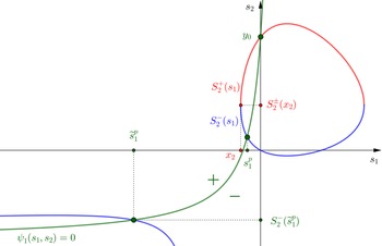
General shape of the curve
 $\{(s_1,s_2)\in{\mathbb{R}}^2\,:\, \psi(s_1,s_2)=0\}$
divided into two parts: the function
 $S_2^-$
(blue) and the function
 $S_2^+$
(red).

Zoom of Figure 4: the branch points
 $x_i$
and
 $y_i$
are in black, and the points
 $x_0$
and
 $y_0$
are in green.

For further use, we define the curve
 \begin{align*}{\mathcal{C}}_1\,:\!=\, S_1^\pm([y_3,y_4])=\left\lbrace\dfrac{-\widetilde{b}(y)\pm i\sqrt{-\widetilde{d}(y)}}{2\widetilde{a}(y)}\,:\, y\in [y_3,y_4]\right\rbrace.\end{align*}
This curve will be the boundary in the BVP established in Section 6.3.
Lemma 6.2 (The circle
 ${\mathcal{C}}_1$
). The curve
 ${\mathcal{C}}_1$
is a circle with centre at
 $-q_1$
and radius
 $\sqrt{\frac{\lambda_1q_1}{c_1}}$
.
Proof. By definition, if
 $s_1\in{\mathcal{C}}_1$
, then there exists
 $s_2\in [y_3,y_4]$
such that
 $\psi(s_1,s_2)=0$
, and we also have
 $\overline{s_1}\in{\mathcal{C}}_1$
and
 $\psi(\overline{s_1},s_2)=0$
. This implies that
 $\psi(s_1,s_2)=\psi(\overline{s_1},s_2)$
; that is,
 \begin{align*}c_1s_1+\dfrac{\lambda_1q_1}{s_1+q_1}=c_1\overline{s_1}+\dfrac{\lambda_1q_1} {\overline{s_1}+q_1}.\end{align*}
Then we find that
 \begin{align*}{\lvert}s_1+q_1{\rvert}^2=\dfrac{\lambda_1q_1}{c_1}.\end{align*}
We deduce that
 ${\mathcal{C}}_1$
is included in the circle with centre
 $-q_1$
and radius
 $\sqrt{\frac{\lambda_1q_1}{c_1}}$
. Furthermore, as
 $S_1^+(y_i)=S_1^-(y_i)$
, this implies that
 ${\mathcal{C}}_1$
is a closed curve, which concludes the proof.
In fact, we may choose the interval
 $[y_1,y_2]$
instead of
 $[y_3,y_4]$
, since
 ${\mathcal{C}}_1=S_1^\pm([y_1,y_2])$
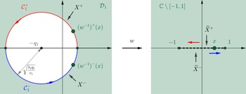
. Finally, we define the domain
 \begin{align*}{\mathcal{D}}_1\,:\!=\,\left\lbrace s_1\in{\mathbb{C}}\,:\, {\lvert}s_1+q_1{\rvert}^2>\dfrac{\lambda_1q_1}{c_1}\right\rbrace,\end{align*}
which is the complement of the disc defined by the circle
 ${\mathcal{C}}_1$
; see Figure 6. We deduce from Lemma 6.1 that
 $x_3,x_4$
are in
 ${\mathcal{D}}_1$
and that
 $x_1,x_2$
are not.
Complex plane of the
 $s_1$
variable: the branch points
 $x_i$
and the cuts on the complex plane are in blue, while the circle
 ${\mathcal{C}}_1$
and the domain
 ${\mathcal{D}}_1$
are in green.

6.2. Analytic continuation and asymptotics
The goal of this section is to analytically continue
 $F_1$
to the domain
 ${\mathcal{D}}_1$
and to study its singularities in order to compute the asymptotics of
 $p_1(u,0)$
and
 $p_1(0,v)$
; see Proposition 6.1.
Lemma 6.3 (Analytic continuation). The function
 $F_1(s_1)$
can be meromorphically extended to the set
 \begin{align*}\{s_1\in{\mathbb{C}}\,:\, \Re s_1>0 \text{ or } \Re S_2^+(s_1)>0\}\end{align*}
thanks to the formula
 \begin{equation}F_1(s_1)=F_1(q_2/r_2)+\dfrac{\psi_2\big(s_1,S_2^+(s_1)\big) \left[F_2(q_1/r_1)-F_2\big(S_2^+(s_1)\big)\right]-F_0}{\psi_1\big(s_1,S_2^+(s_1)\big)}.\end{equation}
The analogous result holds for
 $F_2$
.
Proof. We are going to use the principle of analytic continuation. The Laplace transforms
 $F_i(s)$
are analytic on
 $\{s\in{\mathbb{C}}\,:\, \Re s >0\}$
. According to the kernel equation (5.3), for
 $s_1$
and
 $s_2$
with positive real parts and such that
 $\psi(s_1,s_2)=0$
we have
 \begin{align*}0=\psi_1(s_1,s_2)(F_1(s_1)-F_1(q_2/r_2))+\psi_2(s_1,s_1)(F_2(s_2)-F_2(q_1/r_1))+F_0.\end{align*}
When
 $s_1 \to 0$
for
 $s_1>0$
we have
 $S_2^+(s_1)\to\frac{\lambda_2}{c_2}-q_2=y_0>0$
. Thus the open connected set
 \begin{align*}D\,:\,\big\{s_1\in{\mathbb{C}}\,:\, \Re S_2^+(s_1)>0\big\}\end{align*}
intersects the open set
 $\{s_1\in{\mathbb{C}}\,:\, \Re s_1>0\}$
. For
 $s_1$
in this intersection the equation (6.1) is satisfied. Then, defining
 $F(s_1)$
as in (6.1), we meromorphically extend
 $F_1$
to the whole of D thanks to the principle of analytic continuation. See Figure 7 for an illustration of the domain D.
Representation of the
 $s_1$
-complex plane: the domain
 $D\,:\!=\,\{s_1\in{\mathbb{C}}\,:\, \Re S_2^+(s_1)>0\}$
is in yellow; the red curve is the set
 $\{s_1\in{\mathbb{C}}\,:\, \Re S_2^+(s_1)=0\}$
. The red dotted curve is the set
 $\{s_1\in{\mathbb{C}}\,:\, \Re S_2^-(s_1)=0\}$
(note that we do not use this curve).

Lemma 6.4 (The domain
 ${\mathcal{D}}_1$
). The set
 ${\mathcal{D}}_1$
is included in
 $\{s_1\in{\mathbb{C}}\,:\, \Re s_1>0\text{ or } \Re S_2^+(s_1)>0\}$
, and
 $F_1$
is therefore meromorphic on
 ${\mathcal{D}}_1$
.
Proof. It is enough to show that
 ${\mathcal{D}}_1\cap \{s_1\in{\mathbb{C}}\,:\, \Re s_1<0\} $
is included in the domain D. See Figures 6 and 7 to visualize these sets. By definition, if
 $s_1\in{\mathcal{C}}_1$
, we have
 $S_2^+(s_1)\in [y_3,y_4]$
and then
 $\Re S_2^+(s_1)>0$
. We deduce that the circle
 ${\mathcal{C}}_1$
is included in D. Furthermore, remark that
 \begin{align*}S_2^+(s_1)\underset{{\lvert}s_1{\rvert}\to\infty}{\sim} -\dfrac{c_1}{c_2}s_1,\end{align*}
which implies that when
 $s_1$
is large and such that
 $\Re s_1<0$
we have
 $\Re S_2^+(s_1)>0$
. The maximum principle applied to the function
 $S_2^+(s_1)$
implies that
 $\Re S_2^+(s_1)$
is positive on the set
 ${\mathcal{D}}_1\cap \{s_1\in{\mathbb{C}}\,:\, \Re s_1<0\} $
. We conclude using Lemma 6.3.
Let us recall that
 $x_2$
and
 $y_2$
are the roots defined in Lemma 6.1.
Lemma 6.5 (Poles of
 $F_1$
and
 $F_2$
). The polynomial
 \begin{equation}P(s_1)\,:\!=\, (s_1-q_2/r_2)(s_1+q_1)(r_2c_2-c_1)+\lambda_2(s_1+q_1)+\lambda_1(s_1-q_2/r_2)\end{equation}
has two real roots
 $s_1^p\in ({-}q_1,0)$
and
 $\widetilde{s}_1^p$
when
 $r_2c_2-c_1\neq 0$
and one real root
 $s_1^p\in ({-}q_1,0)$
when
 $r_2c_2-c_1=0$
.
The meromorphic function
 $F_1(s_1)$
has at most two poles in
 $\{s_1\in{\mathbb{C}}\,:\, \Re s_1>0 \text{ or } \Re S_2^+(s_1)>0\}$
, which are 0 and
 $s_1^p$
:
-
0 is always a simple pole of
$F_1$
; -
$s_1^p$
is a (simple) pole of
$F_1$
if and only if
$\psi_1\big(x_2,S_2^\pm(x_2)\big)<0$
.


Furthermore,
 $F_1$
has no poles in
 ${\mathcal{D}}_1$
and is analytic on this set.
In the same way we define
 $s_2^p\in ({-}q_2,0)$
, which is a (the only) pole of
 $F_2$
if and only if
 $\psi_2\big(S_1^\pm(y_2),y_2\big)<0$
.
Proof. The function
 $F_1$
is initially defined as a Laplace transform which converges on
 $\{s_1\in{\mathbb{C}}\,:\, \Re s_1>0\}$
. Thus,
 $F_1$
has no poles on this set. The limits in Theorem 3.1 imply that
 $\hat{F}_1(0+)=1$
(and
 $\hat{F}_2(0+)=0$
), and we deduce that 0 is a simple pole of
 $F_1$
(and that 0 is not a pole of
 $F_2$
). The analytic continuation of
 $F_1$
is obtained thanks to the formula (6.1). Therefore, the only poles of
 $F_1$
come from the values of
 $s_1$
having negative real part such that
 \begin{align*}\psi_1\big(s_1,S_2^+(s_1)\big)=0.\end{align*}
First, we show that the following system has three solutions: 0,
 $s_1^p$
, and
 $\widetilde{s}_1^p$
. We have
 \begin{align*}\begin{cases}\psi(s_1,s_2)=0,\\[4pt]\psi_1(s_1,s_2)=0,\end{cases}\Leftrightarrow\begin{cases}s_1\bigg(c_1-\dfrac{\lambda_1}{q_1+s_1}\bigg)+s_2\bigg(c_2-\dfrac{\lambda_2}{q_2+s_2}\bigg)=0,\\[12pt]-\dfrac{\lambda_2}{(q_2+s_2)}=\dfrac{c_2(s_1r_2-q_2)}{q_2},\end{cases}\\[6pt]\Leftrightarrow\begin{cases}s_1\left(\bigg(c_1-\dfrac{\lambda_1}{q_1+s_1}\bigg)+s_2\dfrac{c_2 r_2}{q_2}\right)=0,\\[12pt]s_2=\dfrac{\lambda_2q_2}{c_2(q_2-s_1r_2)}-q_2,\end{cases}\Leftrightarrow\begin{cases}s_1P(s_1)=0,\\[4pt]s_2=\dfrac{\lambda_2q_2}{c_2(q_2-s_1r_2)}-q_2,\end{cases}\end{align*}
where
 $P(s_1)$
is a second-degree polynomial defined by (6.2). Notice that
 \begin{align*}P(0)=q_1q_2\left(c_1-\dfrac{\lambda_1}{q_1}- r_2\left(c_2-\dfrac{\lambda_2}{q_2}\right)\right)>0,\end{align*}
which is positive thanks to the assumption (A2) (where
 $\mu_i=c_i-\lambda_i/q_i$
), and that
 \begin{align*}P({-}q_1)=-\lambda_1(q_1+q_2/r_2)<0.\end{align*}
We deduce that the two roots of P are real and that one of them, which we denote by
 $s_1^p$
, satisfies
 $-q_1<s_1^p<0$
and then
 $s_1^p\notin{\mathcal{D}}_1$
. We have that
 $s_1^p$
is a (simple) pole of
 $F_1$
if and only if
 $\psi_1\big(s_1^p,S_2^+\big(s_1^p\big)\big)=0$
, i.e.
 $\psi_1\big(x_2,S_2^\pm(x_2)\big)<0$
; see Figure 8 for a geometric representation. We now show that the second root of P, denoted by
 $\widetilde{s}_1^p$
, is not a pole of
 $F_1$
. Firstly, this is clearly the case when
 $\widetilde{s}_1^p>0$
. Secondly,
 $\widetilde{s}_1^p<-q_1<0$
is not a pole of
 $F_1$
, because we have
 $\psi_1\big(\widetilde{s}_1^p,S_2^-\big(\widetilde{s}_1^p\big)\big)=0$
, but
 $\psi_1\big(\widetilde{s}_1^p,S_2^+\big(\widetilde{s}_1^p\big)\big)\neq 0$
; see Figure 8 for a geometric representation.
The curve
 $\psi_1(s_1,s_2)=0$
and its intersections with the curve
 $\psi(s_1,s_2)=0$
are shown in green. In this case,
 $\psi_1\big(x_2,S_2^\pm(x_2)\big)>0$
, and then
 $s_1^p$
is not a pole of
 $F_1$
.

Our next result establishes the rate of decay of
 $p_2(u,0)=1-p_1(u,0)$
. It is noted that the analogous result holds true for
 $p_1(0,v)$
as
 $v\to\infty$
.
Proposition 6.1 (Asymptotics of domination). The asymptotic behaviour of
 $p_1(u,0)$
as
 $u\to\infty$
is given by
 \begin{align*}1-p_1(u,0)\sim C\begin{cases}e^{us_1^p} & \text{ if } \psi_1\big(x_2,S_2^\pm(x_2)\big)<0,\\[3pt]u^{-\frac{3}{2}}e^{u x_2} & \text{ if } \psi_1\big(x_2,S_2^\pm(x_2)\big)>0,\\[3pt]u^{-\frac{1}{2}}e^{u x_2} & \text{ if } \psi_1\big(x_2,S_2^\pm(x_2)\big)=0,\end{cases}\end{align*}
for some constant C which depends on the case, where
 ${s}_1^p$
is defined in Lemma 6.5.
Proof. The asymptotics of a function derives from the largest singularity of its Laplace transform; see for example [Reference Doetsch9, Theorem 37.1]. Assume that f(u) is a function, L(s) is its Laplace transform, and a is the largest singularity of order k (i.e. in the neighbourhood of a the Laplace transform F behaves as
 $(s-a)^{-k}$
up to additive and multiplicative constants). Then apply the theorems stating that f(u) is equivalent to
 $u^{k-1}e^{au}$
up to a constant as
 $u\to\infty$
.
The Laplace transform of interest is
 $1/s_1-F_1(s_1)$
. By Lemma 6.5 the point 0 is not a singularity, whereas
 ${s}_1^p$
is a simple pole and the largest singularity of
 $F_1$
if
 $\psi_1\big(x_2,S_2^\pm(x_2)\big)<0$
. In that case the asymptotics is given by
 $Ce^{us_1^p}$
for some constant C. When
 $\psi_1\big(x_2,S_2^\pm(x_2)\big) \geqslant 0$
, the largest singularity is the branch point
 $x_2$
. Thanks to the definition of
 $S_2^+$
and the analytic continuation formula (6.1) we obtain for some constants
 $C_i$
that
 \begin{align*}F_1(s_1)\underset{s_1\to x_2}{=}\begin{cases}C_1+C_2\sqrt{s_1-x_2}+{\mathrm{O}}(s_1-x_2) & \text{ if } \psi_1\big(x_2,S_2^\pm(x_2)\big)>0,\\[9pt]\dfrac{C_3}{\sqrt{s_1-x_2}}+{\mathrm{O}}(1) & \text{ if } \psi_1\big(x_2,S_2^\pm(x_2)\big)=0.\end{cases}\end{align*}
The result now follows.
6.3. Boundary value problem and its solution
We are now ready to establish a BVP satisfied by
 $f_1$
defined in (5.8). It is a Carleman homogeneous BVP which relies on the domain
 ${\mathcal{D}}_1$
and the boundary
 ${\mathcal{C}}_1$
.
Proposition 6.2 (BVP). The function
 $f_1$
satisfies the following Carleman BVP:
-
(i)
$f_1(s_1)$
is analytic on
${\mathcal{D}}_1$
; -
(ii)
$\lim_{s_1\to\infty} f_1(s_1)=\dfrac{F_0}{\widetilde{F}_0}\dfrac{r_2}{q_2}-F_1(q_2/r_2)$
; -
(iii)
$f_1$
satisfies the boundary condition where
\begin{align*}f_1(\overline{s_1})=G(s_1)f_1(s_1),\quad \forall\; s_1\in{\mathcal{C}}_1,\end{align*}
(6.3)
\begin{equation}G(s_1)\,:\!=\,\dfrac{\psi_1}{\psi_2}\big(s_1,S_2^+(s_1)\big) \dfrac{\psi_2}{\psi_1}\big(\overline{s_1},S_2^+(s_1)\big).\end{equation}


Proof. Item (i) directly derives from Lemma 6.4 and Lemma 6.5. Item (ii) comes from the fact that the Laplace transform
 $F_1$
converges to 0 at infinity. Item (iii) comes from the kernel equation (5.7). For
 $s_1\in{\mathcal{C}}_1$
, we have
 $\overline{s_1}\in{\mathcal{C}}_1$
and
 $S_2^+(s_1)=S_2^+(\overline{s_1})$
. We evaluate (5.7) at
 $\big(s_1,S_2^+(s_1)\big)$
and
 $\big(\overline{s_1},S_2^+(s_1)\big)$
and obtain the two equations
 \begin{align*}\begin{cases}0=\psi_1\big(s_1,S_2^+(s_1)\big)f_1(s_1)+\psi_2\big(s_1,S_2^+(s_1)\big)f_2\big(S_2^+(s_1)\big),\\[4pt]0=\psi_1\big(\overline{s_1},S_2^+(s_1)\big)f_1(\overline{s_1})+ \psi_2\big(\overline{s_1},S_2^+(s_1)\big)f_2\big(S_2^+(s_1)\big).\end{cases}\end{align*}
Eliminating
 $f_2\big(S_2^+(s_1)\big)$
from these equations gives the boundary condition (iii).
To solve the BVP on
 ${\mathcal{D}}_1$
we need to introduce a conformal function which glues together the upper part and the lower part of the circle
 ${\mathcal{C}}_1$
. This gluing function is a simple rational function and derives from the kernel. See Figure 9 to visualize the gluing function.
The conformal gluing function w is one-to-one from
 ${\mathcal{D}}_1$
to
 ${\mathcal{C}}\setminus [{-}1,1]$
.

Lemma 6.6 (Conformal gluing function). The function
 \begin{equation}w(s_1)\,:\!=\,\dfrac{1}{2}\left(\dfrac{s_1+q_1}{\sqrt{\lambda_1q_1/c_1}}+ \dfrac{\sqrt{\lambda_1q_1/c_1}}{s_1+q_1}\right)\end{equation}
satisfies the following properties:
-
(i) w is holomorphic in
${\mathcal{D}}_1$
and continuous on
$\overline{{\mathcal{D}}_1}$
; -
(ii) w is one-to-one from
${\mathcal{D}}_1$
to
${\mathbb{C}}\setminus [{-}1,1]$
; -
(iii) w satisfies the boundary property
\begin{align*}w(s_1)=w(\overline{s_1}),\quad \forall\, s_1\in{\mathcal{C}}_1.\end{align*}


Proof. Recall that
 $s_1\in{\mathcal{C}}_1$
if and only if
 ${\lvert}s_1+q_1{\rvert}^2=\frac{\lambda_1q_1}{c_1}$
. The three items are derived by means of straightforward calculus.
We write
 ${\mathcal{C}}_1^-$
(resp.
 ${\mathcal{C}}_1^+$
) for the half-circle defined by the intersection of
 ${\mathcal{C}}_1$
and the half-plane of negative (resp. positive) imaginary part; see Figure 9. The circle
 ${\mathcal{C}}_1$
and the half-circles
 ${\mathcal{C}}_1^\pm$
are oriented counterclockwise.
To solve the BVP we need to compute the index, which is defined by
 \begin{align*}\chi\,:\!=\,\dfrac{1}{2\pi}[\arg G(s_1)]_{{\mathcal{C}}_1^-}=\dfrac{1}{2\pi} \left[\arg\dfrac{\psi_1}{\psi_2}\big(s_1,S_2^+(s_1)\big)\right]_{{\mathcal{C}}_1}.\end{align*}
The index represents the variation of the argument of
 $G(s_1)$
when
 $s_1$
lies on the half-circle
 ${\mathcal{C}}_1^-$
, that is, the difference between initial and the final value when the argument varies continuously along the half-circle. The second equality comes from the definition of G in (6.3). Thus, equivalently, it is also the variation of the argument of
 $\psi_1/\psi_2$
around the circle
 ${\mathcal{C}}_1$
.
Lemma 6.7 (Index). The index
 $\chi$
is given by
 \begin{equation}\chi=\begin{cases}0\text{ if } q_2/r_2 \leqslant -q_1+\sqrt{\lambda_1q_1/c_1}\Leftrightarrow\ f_1\text{ has no zeros in ${\mathcal{D}}_1$,}\\[5pt]1\text{ if } q_2/r_2>-q_1+\sqrt{\lambda_1q_1/c_1}\Leftrightarrow\ f_1 \text{ has one zero ($q_2/r_2$) in ${\mathcal{D}}_1$.}\end{cases}\end{equation}
Proof. Consider the curve
 $\frac{\psi_1}{\psi_2}\big(s_1,S_2^+(s_1)\big)$
when
 $s_1$
lies on
 ${\mathcal{C}}_1$
. This curve is numerically plotted in Figure 10 in both cases of interest. Let us denote by
 $A=\frac{\psi_1}{\psi_2}\big({-}q_1-\sqrt{\lambda_1q_1/c_1},y_4\big)$
and
 $B=\frac{\psi_1}{\psi_2}\big({-}q_1+\sqrt{\lambda_1q_1/c_1},y_3\big)$
the image under
 $\frac{\psi_1}{\psi_2}$
of the two real points of
 ${\mathcal{C}}_1$
. Analysis of the equation defining this curve shows also that there is another double real point, which we denote by C.
Plot of
 $\frac{\psi_1}{\psi_2}\big(s_1,S_2^+(s_1)\big)$
when
 $s_1$
lies on
 ${\mathcal{C}}_1$
. Left:
 $q_2/r_2\in{\mathcal{D}}_1$
and
 $\chi=1$
; right:
 $q_2/r_2\notin{\mathcal{D}}_1$
and
 $\chi=0$
.

We can show that A and C are always positive. On the other hand
 $B<0$
if and only if
 $q_2/r_2>-q_1+\sqrt{\lambda_1q_1/c_1}$
. The last property comes from the fact that the line
 $s_1=q_2/r_2$
is the asymptote of the hyperbola
 $\psi_1(s_1,s_2)=0$
, and the position of the point
 $\big({-}q_1+\sqrt{\lambda_1q_1/c_1},y_3\big)$
with respect to this asymptote determines the sign of B. Now we see that when
 $q_2/r_2>-q_1+\sqrt{\lambda_1q_1/c_1}$
, the curve of interest makes a positive turn around the origin, i.e.
 $\chi=1$
. In the other case,
 $B>0$
and the curve makes no turns around the origin, i.e.
 $\chi=0$
.
Alternatively, one may start by noticing that by the boundary condition of Proposition 6.2,
 \begin{align*}\chi=\dfrac{1}{2\pi}\left[\arg\dfrac{f_1(\overline{s_1})}{f_1(s_1)}\right]_{{\mathcal{C}}_1^-}=\dfrac{-1}{2\pi}\left[\arg{f_1(s_1)}\right]_{{\mathcal{C}}_1}=Z_{{\mathcal{D}}_1}(f_1)-P_{{\mathcal{D}}_1}(f_1),\end{align*}
where
 $Z_{{\mathcal{D}}_1}(f_1)$
is the number of zeros (counted with multiplicity) of the meromorphic function
 $f_1$
in
 ${\mathcal{D}}_1\cup \{\infty\}$
and
 $P_{{\mathcal{D}}_1}(f_1)$
is the number of poles (counted with multiplicity) of
 $f_1$
in
 ${\mathcal{D}}_1\cup \{\infty\}$
. By Lemma 6.5, the function
 $f_1$
has no poles in
 ${\mathcal{D}}_1\cup \{\infty\}$
, so that
 $\chi \geqslant 0$
; it then remains to analyse the zeros of
 $f_1$
, remembering that
 $f_1(q_2/r_2)=0$
.
We are now ready to present an explicit integral expression for
 $F_1$
. The analogous result holds for
 $F_2$
, and thus we obtain an explicit expression for F via the kernel equation. Recall that G is defined in (6.3), w in (6.4),
 $F_0$
in (5.5), and
 $\widetilde{F}_0$
in (5.8), and that
 $\chi$
is given in (6.5).
Theorem 6.1 (Explicit expression for
 $F_1$
). The Laplace transform
 $F_1$
is given by
 \begin{equation}F_1(s_1)=\dfrac{F_0}{\widetilde{F}_0}\dfrac{1}{s_1}+\left(\dfrac{F_0}{\widetilde{F}_0} \dfrac{r_2}{q_2}-F_1(q_2/r_2)\right)\left(X(s_1)-1\right),\quad \forall\, s_1\in{\mathcal{D}}_1,\end{equation}
where
 \begin{equation}X(s_1)\,:\!=\,\left(\dfrac{w(s_1)-w(q_2/r_2)}{w(s_1)-1}\right)^\chi \exp\left(\dfrac{1}{2i\pi}\int_{{\mathcal{C}}_1^-} \log(G(t))\dfrac{w^{\prime}(t)}{w(t)-w(s_1)}{\mathrm{d}} t\right)\end{equation}
and
 \begin{align*}F_1(q_2/r_2)=\dfrac{F_0}{\widetilde{F}_0}\dfrac{r_2}{q_2}+\dfrac{F_0}{X(x_0)} \left(\dfrac{1}{\widetilde{F}_0}\left(\dfrac{1}{x_0}-\dfrac{r_2}{q_2}\right)+ \dfrac{1}{\psi_1(x_0,0)}\right).\end{align*}
Let us provide some comments. Firstly, the given expression is valid for real
 $s_1$
larger than
 $\sqrt{\lambda_1q_1/c_1}-q_1>0$
. Secondly, we may replace the integral on the half-circle of
 $\log G$
by the integral on the whole circle of
 $\log\frac{\psi_1}{\psi_2}$
, since
 \begin{align*}\int_{{\mathcal{C}}_1^-} \log(G(t))\dfrac{w^{\prime}(t)}{w(t)-w(s_1)}{\mathrm{d}} t=\int_{{\mathcal{C}}_1} \log\left(\dfrac{\psi_1}{\psi_2}\big(t,S_2^+(t)\big)\right)\dfrac{w^{\prime}(t)}{w(t)-w(s_1)}{\mathrm{d}} t.\end{align*}
This theorem establishes the existence of the unique solution of the kernel equation under the limit conditions found in Theorem 3.1. The uniqueness derives from the solution of the BVP and the value of the index. The same remark can be made about Theorem 7.1.
Proof of Theorem 6.1. To solve the Carleman BVP of Proposition 6.2 we are going to transform it into a Riemann BVP using the conformal gluing function w. See, for example, [Reference Fayolle, Iasnogorodski and Malyshev11, Section 5.2] for a brief presentation of the main results of BVP theory. We consider the function
 \begin{align*}\widetilde{f}_1(x)\,:\!=\, (x-w(q_2/r_2))^{-\chi} f_1\circ w^{-1}(x).\end{align*}
According to Proposition 6.2, Lemma 6.6, and the fact that
 $f_1(q_2/r_2)=0$
, we have the following:
-
(i)
$\widetilde{f}_1$
is analytic on
${\mathbb{C}}\setminus [{-}1,1]$
; -
(ii)
$\widetilde{f}_1(x)\underset{\infty}{\sim} x^{-\chi}\left(\frac{F_0}{\widetilde{F}_0} \frac{r_2}{q_2}-F_1(q_2/r_2)\right)$
; -
(iii)
$\widetilde{f}_1$
has left limits
$\widetilde{f}_1^+$
and right limits
$\widetilde{f}_1^-$
on
$[{-}1,1]$
which satisfy the boundary condition with
\begin{align*}\widetilde{f}_1^+(x)=\widetilde{G}(x)\widetilde{f}_1^-(x)\end{align*}
$\widetilde{G}(x)\,:\!=\, G\big(\big(w^{-1}\big)^-(x)\big)$
, where we denote by
$\big(w^{-1}\big)^-$
the right limit on
$[{-}1,1]$
of
$w^{-1}$
; see Figure 9.


The function
 \begin{align*}\widetilde{X}(x)\,:\!=\,\left({x-1}\right)^{-\chi}\exp\left(\dfrac{1}{2i\pi}\int_{-1}^1 \dfrac{\log\widetilde{G}(u)}{u-x}{\mathrm{d}} u\right),\quad \forall\, x\notin{\mathbb{C}}\setminus [0,1],\end{align*}
satisfies the homogeneous problem
 \begin{align*}\widetilde{X}^+(x)=\widetilde{G}(x)\widetilde{X}^-(x),\quad \forall\, x\in [0,1],\end{align*}
where we write
 $\widetilde{X}^+$
(resp.
 $\widetilde{X}^-$
) for the right (resp. left) limit of
 $\widetilde{X}$
on
 $[{-}1,1]$
. This is a classical result of BVP theory stemming from the Sokhotsky–Plemelj formulas; see [Reference Fayolle, Iasnogorodski and Malyshev11, (5.2.24) and Theorem 5.2.3]. We deduce from (iii) that
 \begin{align*}\dfrac{\widetilde{f}_1^+}{\widetilde{X}^+}(x)= \dfrac{\widetilde{f}_1^-}{\widetilde{X}^-}(x),\quad \forall\, x\in [0,1].\end{align*}
From (i) it follows that
 $\frac{\widetilde{f}_1}{\widetilde{X}} $
is analytic on the whole of
 ${\mathbb{C}}$
. Thanks to (ii) and to the fact that
 $\widetilde{X}(x)\sim_\infty x^{-\chi}$
(by Lemma 6.7 and since the integral in the exponential goes to 0 when x goes to infinity), we find that the analytic function
 $\frac{\widetilde{f}_1}{\widetilde{X}}$
converges to
 $\frac{F_0}{\widetilde{F}_0} \frac{r_2}{q_2}-F_1(q_2/r_2)$
at infinity. Thus it coincides with this constant, and so
 \begin{gather*}f_1(s_1)=\left(\dfrac{F_0}{\widetilde{F}_0}\dfrac{r_2}{q_2}-F_1(q_2/r_2)\right) (w(s_1)-w(q_2/r_2))^\chi\widetilde{X}(w(s_1))=\\=\left(\dfrac{F_0}{\widetilde{F}_0}\dfrac{r_2}{q_2}-F_1(q_2/r_2)\right)X(s_1),\end{gather*}
where the last equality follows by the change of variable
 $u=w(t)$
. Now (6.6) follows from the definition of
 $f_1$
in (5.8).
We now compute the constant
 $F_1(q_2/r_2)$
. Equation (5.6) gives
 \begin{align*}F_1(x_0)-F_1(q_2/r_2)=-\dfrac{F_0}{\psi_1(x_0,0)},\end{align*}
whereas (6.6) implies that
 \begin{align*}F_1(x_0)-F_1(q_2/r_2)=\dfrac{F_0}{\widetilde{F}_0} \left(\dfrac{1}{x_0}-\dfrac{r_2}{q_2}\right)+ \left(\dfrac{F_0}{\widetilde{F}_0}\dfrac{r_2}{q_2}-F_1(q_2/r_2)\right)X(x_0),\end{align*}
which readily yields the stated expression for
 $F_1(q_2/r_2)$
.
We conclude by providing an expression for the probability of total domination when starting from the origin.
Corollary 6.1. The probability of total domination when starting from the origin is given by
 \begin{equation}p_1(0,0)=\dfrac{F_0}{\widetilde{F}_0}-\left(\dfrac{F_0}{\widetilde{F}_0}\dfrac{r_2}{q_2}- F_1(q_2/r_2)\right) \dfrac{\sqrt{\lambda_1q_1/c_1}}{i\pi}\int_{{\mathcal{C}}_1^-} \log(G(t))w^{\prime}(t){\mathrm{d}} t.\end{equation}
Proof. We deduce from Theorem 6.1 that
 \begin{align*}p_1(0,0)=\lim_{s_1\to\infty} s_1F_1(s_1)=\dfrac{F_0}{\widetilde{F}_0}+ \left(\dfrac{F_0}{\widetilde{F}_0}\dfrac{r_2}{q_2}-F_1(q_2/r_2)\right)\lim_{s_1\to\infty} s_1(X(s_1)-1).\end{align*}
Let us notice that when
 $s_1\to\infty$
, the integral in the exponential of (6.7) is equivalent to
 $C/s_1$
, where
 \begin{align*}C\,:\!=\, -\dfrac{\sqrt{\lambda_1q_1/c_1}}{i\pi}\int_{{\mathcal{C}}_1^-} \log(G(t))w^{\prime}(t){\mathrm{d}} t.\end{align*}
From the Taylor expansion of X we obtain
 $X(s_1)=1+C/s_1+{\mathrm{o}}(1/s_1)$
, and the result follows.
7. Explicit solution for the Brownian model
In this section we solve the kernel equation (5.11) for the correlated Brownian model. We obtain an explicit integral expression for
 $F_1$
and the probability
 $p_1(0,0)$
in Theorem 7.1. The asymptotics of
 $p_1(u,0)$
,
 $u\to\infty$
, is given in Proposition 7.1. We follow the same steps as in the Poissonian model studied in Section 6; consequently, some details will be omitted. Importantly, the kernel
 $\psi$
is similar to the one studied in [Reference Baccelli and Fayolle2, Reference Franceschi and Raschel14], and so its various properties can be taken from there.
Without stating it explicitly, we assume in the following that our parameters satisfy the conditions of Proposition 5.2. In particular, the correlation is non-negative:
 $\rho\in [0,1)$
. We stress, however, that the main parts of the following analysis can be carried out also for
 $\rho<0$
, and so the remaining hurdle is to show that the same kernel equation holds in this case as well.
7.1. Study of the kernel
Again consider the kernel in (5.11), and define the bi-valued functions
 $S_1$
and
 $S_2$
such that
 \begin{align*}\psi(S_1(s_2),s_2)=0\quad \text{and}\quad \psi(s_1,S_2(s_1))=0.\end{align*}
A direct calculation yields the branches
 \begin{align*}\begin{cases}S_1^\pm(s_2)=\dfrac{-\big(\rho\sigma_1\sigma_2s_2+\mu_1\big)\pm \sqrt{s_2^2\sigma_1^2\sigma_2^2\big(\rho^2-1\big)+ 2s_2\sigma_1(\mu_1\rho\sigma_2-\mu_2\sigma_1)+\mu_1^2}}{\sigma_1^2},\\[12pt]S_2^\pm(s_1)=\dfrac{-\big(\rho\sigma_1\sigma_2s_1+\mu_2\big)\pm \sqrt{s_1^2\sigma_1^2\sigma_2^2\big(\rho^2-1\big)+ 2s_1\sigma_2(\mu_2\rho\sigma_1-\mu_1\sigma_2)+\mu_2^2}}{\sigma_2^2}.\end{cases}\end{align*}
The respective branch points of
 $S_1$
and
 $S_2$
are
 \begin{align*}\begin{cases}y^\pm=\dfrac{\mu_1\rho\sigma_1\sigma_2-\mu_2\sigma_1^2\pm \sqrt{\big(\mu_1\rho\sigma_1\sigma_2-\mu_2\sigma_1^2\big)^2+\mu_1^2\sigma_1^2\sigma_2^2\big(1-\rho^2\big)}} {\sigma_1^2\sigma_2^2\big(1-\rho^2\big)},\\[12pt]x^\pm=\dfrac{\mu_2\rho\sigma_1\sigma_2-\mu_1\sigma_2^2\pm \sqrt{\big(\mu_2\rho\sigma_1\sigma_2-\mu_1\sigma_2^2\big)^2+\mu_2^2\sigma_1^2\sigma_2^2\big(1-\rho^2\big)}} {\sigma_1^2\sigma_2^2\big(1-\rho^2\big)} .\end{cases}\end{align*}
The functions
 $S_1^\pm$
(resp.
 $S_2^\pm$
) are analytic on the cut plane
 ${\mathbb{C}}\setminus (({-}\infty,y^-]\cup [y^+,\infty))$
(resp.
 ${\mathbb{C}}\setminus (({-}\infty,x^-]\cup [x^+,\infty))$
). See Figure 11 to visualize
 $S_2^\pm$
on
 $[x^-,x^+]$
.
The set
 $\{(s_1,s_2)\in{\mathbb{R}}^2\,:\, \psi(s_1,s_2)=0\}$
is an ellipse divided in two parts: the function
 $S_2^-$
(in blue) and the function
 $S_2^+$
(in red). The two lines are the sets defined by
 $\psi_1=0$
and
 $\psi_2=0$
. The branch points
 $x^\pm$
and
 $y^\pm$
are in black, the points
 $x_0$
and
 $y_0$
in green, and the pole
 $s_1^p$
in orange.

Recall the definition of
 $x_0,y_0$
in (5.13). Furthermore, we define
 $s_1^p$
as the first coordinate of the other intersection between the ellipse
 $\psi=0$
and the line
 $\psi_1=0$
. Symmetrically we define
 $s_2^p$
. We have
 \begin{equation}s_1^p\,:\!=\, -\dfrac{2(r_2{\lvert}\mu_2{\rvert}-{\lvert}\mu_1{\rvert})} {\sigma_1^2+\sigma_2^2r_2^2-2\rho\sigma_1\sigma_2r_2}<0\quad \text{and}\quad s_2^p\,:\!=\, -\dfrac{2(r_1{\lvert}\mu_1{\rvert}-{\lvert}\mu_2{\rvert})} {\sigma_2^2+\sigma_1^2r_1^2-2\rho\sigma_1\sigma_2r_1}<0.\end{equation}
See Figure 11 for a geometric interpretation of
 $x_0$
,
 $y_0$
, and
 $s_1^p$
.
We now define the curve
 \begin{align*}{\mathcal{H}}_1\,:\!=\, S_1^\pm([y^+,\infty))=\{s_1\in{\mathbb{C}}\,:\, \psi(s_1,s_2)=0 \text{ and } s_2\in [y^+,\infty)\}.\end{align*}
This curve is the boundary of the BVP established in Section 7.3.
Lemma 7.1 (The hyperbola
 ${\mathcal{H}}_1$
). The curve
 ${\mathcal{H}}_1$
is a branch of a hyperbola that is symmetrical with respect to the horizontal axis, whose equation is
 \begin{equation*}\sigma_1^2\sigma_2^2\big(\rho^2-1\big)x^2+\rho^2\sigma_1^2\sigma_2^2y^2- 2\big(\sigma_2^2\mu_1-\rho\sigma_1\sigma_2\mu_2\big)x= \mu_1\big(\sigma_2^2\mu_1-2\rho\sigma_1\sigma_2\mu_2\big)/\sigma_1^2.\end{equation*}
The curve
 ${\mathcal{H}}_1$
is the right branch of the hyperbola if
 $\rho<0$
, the left branch if
 $\rho>0$
, and a straight line when
 $\rho=0$
; see Figure 12.
Complex plane of the
 $s_1$
variable, with the hyperbola
 ${\mathcal{H}}_1$
and the domain
 ${\mathcal{G}}_1$
in green.

Proof. See [Reference Franceschi and Raschel14, Lemma 4] or [Reference Baccelli and Fayolle2, Lemma 9] which study a similar kernel and derive the equation of the hyperbola.
We denote by
 ${\mathcal{H}}_1^-$
the part of
 ${\mathcal{H}}_1$
with negative imaginary part. Finally we define the domain
 ${\mathcal{G}}_1$
which is bounded by
 ${\mathcal{H}}_1$
and contains
 $x^+$
(and not
 $x^-$
); see Figure 12.
7.2. Asymptotic results
Similarly to Section 6.2, we meromorphically continue
 $f_1$
and study its poles in order to compute the asymptotics of
 $p_1(u,0)$
and
 $p_1(0,v)$
when
 $u\to\infty$
and
 $v\to\infty$
.
Lemma 7.2 (Analytic continuation). The function
 $F_1(s_1)$
can be meromorphically extended to the set
 \begin{equation}\big\{s_1\in{\mathbb{C}}\,:\,\Re s_1>0 \text{ or } \Re S_2^+(s_1)>0\big\}\end{equation}
thanks to the formula
 \begin{equation}F_1(s_1)=\dfrac{-\psi_2\big(s_1,S_2^+(s_1)\big)F_2\big(S_2^+(s_1)\big)-cp_1(0,0)}{\psi_1\big(s_1,S_2^+(s_1)\big)}.\end{equation}
The domain
 ${\mathcal{G}}_1$
is included in the set defined in (7.2), and
 $F_1$
is therefore meromorphic on
 ${\mathcal{G}}_1$
.
Proof. The proof follows the same steps as the proof of Lemma 6.3 and Lemma 6.4. See also [Reference Franceschi and Raschel14, Lemma 5] to show the inclusion of
 ${\mathcal{G}}_1$
in the set defined in (7.2).
Lemma 7.3 (Poles of
 $F_1$
).
 $F_1$
has one or two poles in the set defined in (7.2):
-
0 is always a simple pole of
$F_1$
; -
$s_1^p$
is a simple pole of
$F_1$
if and only if
$\psi_1\big(x^-,S_2^\pm(x^-)\big)<0$
, where
$s_1^p$
is defined in (7.1).


 $F_2$
has a unique simple pole, which is
 $s_2^p$
, if
 $\psi_2\big(S_1^\pm(y^-),y^-\big)<0$
; it has no poles otherwise.
Proof. The proof follows the same steps as the proof of Lemma 6.5 (but is simpler). The poles come from the zeros of the denominator of the continuation formula (7.3), that is, the zeros of
 $\psi_1\big(s_1,S_2^+(s_1)\big)$
. It is the intersection between a line and an ellipse; see Figure 11.
Proposition 7.1 (Asymptotics of domination). The asymptotic behaviour of
 $1-p_1(u,0)$
as
 $u\to\infty$
is given by
 \begin{align*}1-p_1(u,0)\sim C\begin{cases}e^{us_1^p} & \text{ if } \psi_1\big(x^-,S_2^\pm(x^-)\big)<0,\\[4pt]u^{-\frac{3}{2}}e^{ux^-} & \text{ if } \psi_1\big(x^-,S_2^\pm(x^-)\big)>0,\\[4pt]u^{-\frac{1}{2}}e^{ux^-} & \text{ if } \psi_1\big(x^-,S_2^\pm(x^-)\big)=0,\end{cases}\end{align*}
for some constant C which depends on the case, where
 $s_1^p$
is defined in (7.1).

7.3. Boundary value problem and its solution
We state a homogeneous Carleman BVP satisfied by the function
 $f_1$
defined in (5.17).
Proposition 7.2 (BVP). The function
 $f_1$
satisfies the following Carleman BVP:
-
(i)
$f_1(s_1)$
is analytic on
${\mathcal{G}}_1$
; -
(ii)
$\lim_{s_1\to\infty} f_1(s_1)=0$
; -
(iii)
$f_1$
satisfies the boundary condition on the hyperbola where
\begin{align*}f_1(\overline{s_1})=G(s_1)f_1(s_1),\quad \forall\, s_1\in{\mathcal{H}}_1,\end{align*}
(7.4)
\begin{equation}G(s_1)\,:\!=\,\dfrac{\psi_1}{\psi_2}\big(s_1,S_2^+(s_1)\big) \dfrac{\psi_2}{\psi_1}\big(\overline{s_1},S_2^+(s_1)\big).\end{equation}


Proof. The proof follows the same steps as that of Proposition 6.2.
Following [Reference Franceschi and Raschel13, Reference Franceschi and Raschel14] we are going to define the conformal gluing function which glues together the upper part of the hyperbola and its lower part. To that end we define for
 $a \geqslant 0$
the generalized Chebyshev polynomial for
 $x\in{\mathbb{C}}\setminus ({-}\infty,-1]$
by
 \begin{align*}T_a(x)\,:\!=\,\cos(a\arccos(x))=\dfrac{1}{2}\left(\left(x+\sqrt{x^2-1}\right)^a+ \left(x-\sqrt{x^2-1}\right)^a\right).\end{align*}
Let us also define the angle of the model
 \begin{align*}\beta\,:\!=\,\arccos({-}\rho).\end{align*}
Lemma 7.4 (Conformal gluing function). The function
 \begin{equation}W(s_1)\,:\!=\, T_{\frac{\pi}{\beta}}\left(\dfrac{2s_1-(x^++x^-)}{x^+-x^-}\right)\end{equation}
satisfies the following properties:
-
(i) W is holomorphic in
${\mathcal{G}}_1$
and continuous on
$\overline{{\mathcal{G}}_1}$
; -
(ii) W is injective in
${\mathcal{G}}_1$
; -
(iii) W satisfies the boundary property
\begin{align*}W(s_1)=W(\overline{s_1}),\quad \forall\, s_1\in{\mathcal{H}}_1.\end{align*}


Proof. This function has already been studied in several papers. See, for example, [Reference Franceschi and Raschel13, Lemma 3.4] and also [Reference Foschini12, Figure 3] in the case of symmetric conditions.
To state the main theorem of this section we define
 \begin{equation*}\kappa_1\,:\!=\,\begin{cases}1 & \text{if } 0>S_1^\pm(y^+),\\[4pt]0 & \text{if } 0 \leqslant S_1^\pm(y^+),\end{cases}\quad \text{and}\quad \kappa_2\,:\!=\,\begin{cases}1 & \text{if } \psi_1\big(x^-,S_2^\pm(x^-)\big)<0 \text{ and } s_1^p>S_1^\pm(y^+),\\[4pt]0 & \text{otherwise.}\end{cases}\end{equation*}
Using Lemma 7.3 we note that
 $\kappa_1$
is defined so that
 $\kappa_1=1$
when the pole 0 of
 $F_1$
is in
 ${\mathcal{G}}_1$
, and
 $\kappa_1=0$
otherwise. In the same way
 $\kappa_2=1$
when
 $s_1^p$
is a pole and is in
 ${\mathcal{G}}_1$
, and
 $\kappa_2=0$
otherwise.
Let us recall that W is defined in (7.5), G in (7.4),
 ${\mathcal{H}}_1^-$
in Lemma 7.1, and c in (5.12).
Theorem 7.1 (Explicit expression for
 $F_1$
). The Laplace transform
 $F_1$
is given by
 \begin{equation}F_1(s_1)=p_1(0,0)\left(\dfrac{1}{s_1}+CX(s_1)\right),\quad s_1\in{\mathcal{G}}_1,\end{equation}
where
 \begin{align}X(s_1)\unicode{x2254} \left(\dfrac{1}{W(s_1)-W(0)}\right)^{\kappa_1} &\left(\dfrac{1}{W(s_1)-W\big(s_1^p\big)}\right)^{\kappa_2}\\ &\quad \quad \quad \quad \quad \quad \times\exp\left(\dfrac{1}{2i\pi} \int_{{\mathcal{H}}_1^-} \log(G(t))\dfrac{W^{\prime}(t)}{W(t)-W(s_1)}{\mathrm{d}} t\right),\end{align}
 \begin{equation}C\,:\!=\, -\dfrac{1}{X(x_0)}\left(\dfrac{1}{x_0}+\dfrac{c}{\psi_1(x_0,0)}\right).\end{equation}
Furthermore,
 $p_1(0,0)$
is given by Corollary 5.1 for
 $\rho=0$
, whereas for
 $\rho\in\big(0,\frac{1}{2}\frac{\sigma_2\mu_1}{\sigma_1\mu_2}\big)$
we have
 \begin{align}p_1(0,0)=\dfrac{\frac{1}{2}\sigma^2_2\big(r_2-\mu_1/\mu_2\big)\psi_2\big(S_1^+(y_0),y_0\big)} {c(\psi_2\big(S_1^+(y_0),y_0\big)-\psi_2(0,y_0))-\psi_2(0,y_0)\psi_1\big(S_1^+(y_0),y_0\big) \left(1/S_1^+(y_0)+CX\big(S_1^+(y_0)\big)\right)},\nonumber\\[5pt]\end{align}
and for
 $\rho\in\big[\frac{1}{2}\frac{\sigma_2\mu_1}{\sigma_1\mu_2},1\big)$
we have
 \begin{equation}p_1(0,0)=\dfrac{1}{1+C\lim_{s_1\to 0} s_1X(s_1)},\end{equation}
where
 \begin{align}\lim_{s_1\to 0} s_1X(s_1)=\dfrac{1}{W^{\prime}(0)}&\left(\dfrac{1}{W(0)-W\big(s_1^p\big)}\right)^{\kappa_2}\\ &\quad\quad\quad\quad\quad \times\exp\left(\dfrac{1}{2i\pi}\int_{{\mathcal{H}}_1^-} \log(G(t))\dfrac{W^{\prime}(t)}{W(t)-W(0)}{\mathrm{d}} t\right).\end{align}
Proof. The proof follows the same steps as that of Theorem 6.1 and also that of [Reference Franceschi and Raschel14, Theorem 1]. Solving the BVP of Proposition 7.2 in a standard way, we find that there exists a constant C’ such that
 \begin{align*}F_1(s_1)=\dfrac{p_1(0,0)}{s_1}+C^{\prime}X(s_1).\end{align*}
We now compute the value of C’. Taking the limit of the kernel equation in
 $(x_0,0)$
(as in the proof of Lemma 5.1), we obtain that
 \begin{align*}0=\psi_1(x_0,0)F_1(x_0)+cp_1(0,0).\end{align*}
Combining this equation with the fact that
 \begin{align*}F_1(x_0)=\frac{p_1(0,0)}{x_0}+C^{\prime}X(x_0),\end{align*}
we deduce that
 $C^{\prime}=Cp_1(0,0)$
, where C is defined in (7.8), and we obtain (7.6).
It remains to find
 $p_1(0,0)$
in the case
 $\rho\in (0,1)$
. First, it is important to note that
 $S_1^+(y_0)\in{\mathcal{G}}_1\cap [0,\infty)$
. The positivity is easy to see because
 \begin{align*}S_1^+(y_0)=\dfrac{2\mu_2\rho\sigma_1/\sigma_2-\mu_1+ \sqrt{(2\mu_2\rho\sigma_1/\sigma_2-\mu_1)^2}}{\sigma_1^2} \geqslant 0,\end{align*}
and
 $S_1^+(y_0)\in{\mathcal{G}}_1$
, because
 \begin{align*}S_1^+(y_0)-S_1^+(y_+)=\dfrac{\rho\sigma_1\sigma_2(y^+-y_0)+ \sqrt{(\mu_1-2\mu_2\rho\sigma_1/\sigma_2)^2}}{\sigma_1^2} \geqslant 0\end{align*}
as
 $y^+-y_0 \geqslant 0$
. We see that
 $S_1^+(y_0)=0$
if and only if
 $\rho \geqslant \frac{1}{2} \frac{\sigma_2\mu_1}{\sigma_1\mu_2}$
.
First assume that
 $S_1^+(y_0)=0$
. We obtain with (7.6)
 \begin{align*}1=\lim_{s_1\to 0} s_1F_1(s_1)=p_1(0,0)\left(1+C\lim_{s_1\to 0} s_1X(s_1)\right),\end{align*}
which gives (7.10). In this case
 $\kappa_1=1$
and we obtain (7.11).
Assume now that
 $S_1^+(y_0)>0$
. As in the proof of Corollary 5.1 we evaluate the kernel equation at
 $(0+,y_0)$
. We get the same (5.15), even though initially the term
 $\rho\sigma_1\sigma_2$
appears on both sides. The second equation is obtained by using the point
 $\big(S_1^+(y_0),y_0\big)$
:
 \begin{align*}0=\psi_1\big(S_1^+(y_0),y_0\big)F_1\big(S_1^+(y_0)\big)+\psi_2\big(S_1^+(y_0),y_0\big)F_2(y_0)+cp_1(0,0).\end{align*}
The third equation we need is (7.6) with
 $s_1=S_1^+(y_0)$
:
 \begin{align*}F_1\big(S_1^+(y_0)\big)=p_1(0,0)\left(\dfrac{1}{S_1^+(y_0)}+CX\big(S_1^+(y_0)\big)\right).\end{align*}
Solving these three linear equations with the three unknowns
 $p_1(0,0)$
,
 $F_2(y_0)$
, and
 $F_1\big(S_1^+(y_0)\big)$
, we obtain (7.9).
8. Numerical illustrations
This section provides numerical illustrations of some of our basic formulas. That is, we consider
 $p_1(0,0)$
, the probability of domination by the first component when starting at the origin, for both (i) the Poisson model (see (6.8)) and (ii) the Brownian model (see (7.9)). The computations were performed using Mathematica and the R programming language. It must be mentioned that numerical evaluation of the contour integrals involved is not a straightforward task, and a certain care should be taken with the branches of the complex logarithm and the square root.
Figure 13 presents plots of
 $p_1(0,0)$
(in green) as a function of the reflection parameter
 $r_2>0.5$
. For both models we take
 $r_1=2.5$
and
 $X_1(1)$
,
 $X_2(1)$
with unit variances and the means
 $\mu_1=-1$
,
 $\mu_2=-2$
. More precisely, in the Poisson model we take
 $c_1=c_2=1$
,
 $\lambda_1=8$
,
 $\lambda_2=18$
,
 $q_1=4$
,
 $q_2=6$
. In the Brownian model we take correlation
 $\rho=0.2$
. It must be mentioned that we use (7.9) and not (7.10), since
 $\rho<1/4$
. Furthermore, the rates in the Poisson model are rather high, which suggest that the respective uncorrelated Brownian approximation should be close; see Section 4.3. In fact, the corresponding curve drawn based on the explicit expression in (5.14) almost coincides with the green curve in Figure 13(a).


In order to check our numerical results, we also perform a Monte Carlo simulation (red dots). It should be stressed that our simulation involves various sources of errors. Firstly, a single run is terminated when
 $Y_1>100$
and
 $Y_2/Y_1<0.1$
(at the time of a jump) or the analogous condition is satisfied with the indices swapped. In the first/second case we assume that the first/second component dominates. The Poisson simulation is otherwise exact, whereas the Brownian model is discretized with time-step
 $0.01$
, so that we reflect a random walk with the corresponding normal increments. In this regard, it is noted that an approximation result similar to that in Section 4 can also be established for random walks. Finally, each value is obtained from 10,000 independent realizations, and thus the 95% asymptotic confidence interval corresponds to
 $\pm 0.02\sqrt{p_1(1-p_1)}$
.
Appendix A. Derivation of the kernel equation for the Poisson model with common jumps
Proof of Proposition 5.3. For the sake of brevity, here we consider only the case when
 $r_1\sigma_1>\sigma_2$
and
 $r_2\sigma_2>\sigma_1$
; the derivation of the kernel equations for other cases is similar (the cases with equalities should be considered separately or treated by approximation).
Let A denote the event that the first coordinate dominates the second one. Obviously, for any
 $u,v>0$
and
 $h>0$
we have
 \begin{equation*}\begin{gathered}\begin{aligned}p_1(u,v)={\mathbb{P}}_{(u,v)}(A)&={\mathbb{P}}_{(u,v)}(A\cap\{\text{X makes at most one jump on [0,h]}\})\\&+{\mathbb{P}}_{(u,v)}(A\cap\{\text{X makes at least two jumps on [0,h]}\}).\end{aligned}\end{gathered}\end{equation*}
It is easy to see that the second term is
 ${\mathrm{O}}(h^2)={\mathrm{o}}(h)$
as
 $h\to 0+$
, uniformly in (u,v).
Now fix arbitrary
 $u,v>0$
. Using the Markov property and considering all possible cases with at most one jump on the time interval [0,h], we obtain
 \begin{align*}p_1(u,v)&=(1-\lambda h)\big(1-\lambda_1h\big)\big(1-\lambda_2h\big)p_1(u+c_1h,v+c_2h)\\&+\lambda h\big(1-\lambda_1h\big)\big(1-\lambda_2h\big)\int\limits_0^{({\overline{q}}_1u)\wedge ({\overline{q}}_2v)} {\mathrm{d}} x\; p_1\big(u-x/{\overline{q}}_1,v-x/{\overline{q}}_2\big)\cdot e^{-x}\\&+\lambda h\big(1-\lambda_1h\big)\big(1-\lambda_2h\big)\int\limits_{{\overline{q}}_2v}^{{\overline{q}}_1u}{\mathrm{d}} x\; p_1\big(u-x/{\overline{q}}_1+r_2\big(x/{\overline{q}}_2-v\big),0\big)\cdot e^{-x}\cdot{1\negmedspace\mathrm{I}}\left\lbrace{\overline{q}}_1u> {\overline{q}}_2v\right\rbrace\\&+\lambda h\big(1-\lambda_1h\big)\big(1-\lambda_2h\big)\int\limits_{{\overline{q}}_1u}^{{\overline{q}}_2v}{\mathrm{d}} x\; p_1\big(0,v-x/{\overline{q}}_2+r_1\big(x/{\overline{q}}_1-u\big)\big)\cdot e^{-x}\cdot{1\negmedspace\mathrm{I}}\left\lbrace{\overline{q}}_2v> {\overline{q}}_1u\right\rbrace\\&+\lambda h\big(1-\lambda_1h\big)\big(1-\lambda_2h\big)\int\limits_{{\overline{q}}_1u}^\infty{\mathrm{d}} x\; p_1\big(u-x/{\overline{q}}_1+r_2\big(x/{\overline{q}}_2-v\big),0\big)\cdot e^{-x}\\&\times{1\negmedspace\mathrm{I}}\left\lbrace r_1u-v>\big(r_1/{\overline{q}}_1-1/{\overline{q}}_2\big)x,\; {\overline{q}}_1u>{\overline{q}}_2v\right\rbrace\\&+\lambda h\big(1-\lambda_1h\big)\big(1-\lambda_2h\big)\int\limits_{{\overline{q}}_2v}^\infty{\mathrm{d}} x\; p_1\big(0,v-x/{\overline{q}}_2+r_1\big(x/{\overline{q}}_1-u\big)\big)\cdot e^{-x}\\&\times{1\negmedspace\mathrm{I}}\left\lbrace r_2v-u>\big(r_2/{\overline{q}}_2-1/{\overline{q}}_1\big)x,\; {\overline{q}}_2v>{\overline{q}}_1u\right\rbrace\\&+\lambda h\big(1-\lambda_1h\big)\big(1-\lambda_2h\big)\int\limits_{{\overline{q}}_1u}^\infty{\mathrm{d}} x\; p_1(0,0)\cdot e^{-x}{\cdot}{1\negmedspace\mathrm{I}}\!\!\left\lbrace \big(r_1/{\overline{q}}_1-1/{\overline{q}}_2\big)x \geqslant r_1u-v,\; {\overline{q}}_1u>{\overline{q}}_2v\right\rbrace\\&+\lambda h\big(1-\lambda_1h\big)\big(1-\lambda_2h\big)\int\limits_{{\overline{q}}_2v}^\infty{\mathrm{d}} x\; p_1(0,0)\cdot e^{-x}{\cdot}{1\negmedspace\mathrm{I}}\!\!\left\lbrace \big(r_2/{\overline{q}}_2-1/{\overline{q}}_1\big)x \geqslant r_2v-u,\; {\overline{q}}_2v>{\overline{q}}_1u\right\rbrace\\&+\lambda_1h(1-\lambda h)\big(1-\lambda_2h\big)\int\limits_0^{q_1u}{\mathrm{d}} x\; p_1(u-x/q_1,v)\cdot e^{-x}\\&+\lambda_1h(1-\lambda h)\big(1-\lambda_2h\big)\int\limits_{q_1u}^\infty{\mathrm{d}} x\; p_1(0,v+r_1(x/q_1-u))\cdot e^{-x}\\&+\lambda_2h\big(1-\lambda_1h\big)(1-\lambda h)\int\limits_0^{q_2v}{\mathrm{d}} x\; p_1(u,v-y/q_2)\cdot e^{-x}\\&+\lambda_2h\big(1-\lambda_1h\big)(1-\lambda h)\int\limits_{q_2v}^\infty{\mathrm{d}} x\; p_1(u+r_2(x/q_2-v),0)\cdot e^{-x}\\&+{\mathrm{o}}(h),\quad h\to 0+.\end{align*}
Multiplying both sides by
 $e^{-s_1u-s_2v}$
and integrating the result over
 $[0,\infty)\times [0,\infty)$
with respect to the variables u and v, we obtain
 \begin{gather*}\int\limits_0^\infty \!\int\limits_0^\infty p_1(u,v)\cdot e^{-s_1u-s_2v}{\mathrm{d}} u{\mathrm{d}} v= (1-(\lambda+\lambda_1+\lambda_2)h)\int\limits_0^\infty \!\int\limits_0^\infty p_1(u+c_1h,v+c_2h)\cdot e^{-s_1u-s_2v}{\mathrm{d}} u{\mathrm{d}} v\\+\lambda h(I_1+I_2+I_3+I_4+I_5+I_6+I_7)+\lambda_1h(I_8+I_9)+ \lambda_2h(I_{10}+I_{11})+{\mathrm{o}}(h),\quad h\to 0+.\end{gather*}
Noting that
 \begin{gather*}\int\limits_0^\infty \!\int\limits_0^\infty p_1(u,v)\cdot e^{-s_1u-s_2v}{\mathrm{d}} u{\mathrm{d}} v-(1-(\lambda+\lambda_1+\lambda_2)h)\int\limits_0^\infty \!\int\limits_0^\infty p_1(u+c_1h,v+c_2h)\cdot e^{-s_1u-s_2v}{\mathrm{d}} u{\mathrm{d}} v\\=\int\limits_{c_1h}^\infty \int\limits_{c_2h}^\infty p_1(u,v)\cdot e^{-s_1u-s_2v}{\mathrm{d}} u{\mathrm{d}} v+ \int\limits_{c_1h}^\infty \int\limits_0^{c_2h} p_1(u,v)\cdot e^{-s_1u-s_2v}{\mathrm{d}} u{\mathrm{d}} v\\+\int\limits_0^{c_1h} \int\limits_{c_2h}^\infty p_1(u,v)\cdot e^{-s_1u-s_2v}{\mathrm{d}} u{\mathrm{d}} v+ \int\limits_0^{c_1h} \int\limits_0^{c_2h} p_1(u,v)\cdot e^{-s_1u-s_2v}{\mathrm{d}} u{\mathrm{d}} v\\-e^{s_1c_1h+s_2c_2h}\int\limits_{c_1h}^\infty \int\limits_{c_2h}^\infty p_1(u,v)\cdot e^{-s_1u-s_2v}{\mathrm{d}} u{\mathrm{d}} v\\+(\lambda+\lambda_1+\lambda_2)he^{s_1c_1h+s_2c_2h}\int\limits_{c_1h}^\infty \int\limits_{c_2h}^\infty p_1(u,v)\cdot e^{-s_1u-s_2v}{\mathrm{d}} u{\mathrm{d}} v\\=\left[(\lambda+\lambda_1+\lambda_2-s_1c_1-s_2c_2)F(s_1,s_2)+c_2F_1(s_1)+c_1F_2(s_2)\right]h+{\mathrm{o}}(h),\end{gather*}
we conclude that
 \begin{equation}\begin{split}(\lambda+\lambda_1+\lambda_2-s_1c_1-s_2c_2)F(s_1,s_2)+c_2F_1(s_1)+c_1F_2(s_2)\\=\lambda(I_1+I_2+I_3+I_4+I_5+I_6+I_7)+\lambda_1(I_8+I_9)+\lambda_2(I_{10}+I_{11}).\end{split}\end{equation}
To compute
 $I_i$
,
 $i=1,\ldots,11$
, we will repeatedly use Fubini’s theorem and suitable changes of variables without mention.
For
 $I_1$
we have
 \begin{align*}I_1& =\int\limits_0^\infty {\mathrm{d}} u \int\limits_0^\infty {\mathrm{d}} v \int\limits_0^{({\overline{q}}_1u)\wedge ({\overline{q}}_2v)} {\mathrm{d}} x\; p_1\big(u-x/{\overline{q}}_1,v-x/{\overline{q}}_2\big)\cdot e^{-x-s_1u-s_2v}\\& =\int\limits_0^\infty {\mathrm{d}} u \int\limits_0^{{\overline{q}}_1u/{\overline{q}}_2} {\mathrm{d}} v \int\limits_0^{{\overline{q}}_2v} {\mathrm{d}} x\; p_1\big(u-x/{\overline{q}}_1,v-x/{\overline{q}}_2\big)\cdot e^{-x-s_1u-s_2v}\\& \quad +\int\limits_0^\infty {\mathrm{d}} u \int\limits_{{\overline{q}}_1u/{\overline{q}}_2}^\infty {\mathrm{d}} v \int\limits_0^{{\overline{q}}_1u} {\mathrm{d}} x\; p_1\big(u-x/{\overline{q}}_1,v-x/{\overline{q}}_2\big)\cdot e^{-x-s_1u-s_2v}=: I^{\prime}_1+I^{\prime\prime}_1.\end{align*}
However,
 \begin{align*}I^{\prime}_1 & =\int\limits_0^\infty {\mathrm{d}} u \int\limits_0^{{\overline{q}}_1u/{\overline{q}}_2} {\mathrm{d}} v \int\limits_0^{{\overline{q}}_2v} {\mathrm{d}} x\; p_1\big(u-x/{\overline{q}}_1,v-x/{\overline{q}}_2\big)\cdot e^{-x-s_1u-s_2v}\\& ={\overline{q}}_2\int\limits_0^\infty {\mathrm{d}} u \int\limits_0^{{\overline{q}}_1u/{\overline{q}}_2} {\mathrm{d}} v \int\limits_0^v {\mathrm{d}} z\; p_1\big(u-{\overline{q}}_2(v-z)/{\overline{q}}_1,z\big)\cdot e^{-{\overline{q}}_2(v-z)-s_1u-s_2v}\\& ={\overline{q}}_2\int\limits_0^\infty {\mathrm{d}} v \int\limits_0^v {\mathrm{d}} z \int\limits_{{\overline{q}}_2v/{\overline{q}}_1}^\infty {\mathrm{d}} u\; p_1\big(u-{\overline{q}}_2(v-z)/{\overline{q}}_1,z\big)\cdot e^{-{\overline{q}}_2(v-z)-s_1u-s_2v}\\& ={\overline{q}}_2\int\limits_0^\infty {\mathrm{d}} v \int\limits_0^v {\mathrm{d}} z \int\limits_{{\overline{q}}_2z/{\overline{q}}_1}^\infty {\mathrm{d}} y\; p_1(y,z)\cdot e^{-{\overline{q}}_2(v-z)-s_1(y+{\overline{q}}_2(v-z)/{\overline{q}}_1)-s_2v}\\& ={\overline{q}}_2\int\limits_0^\infty {\mathrm{d}} z \int\limits_{{\overline{q}}_2z/{\overline{q}}_1}^\infty {\mathrm{d}} y \int\limits_z^\infty {\mathrm{d}} v\; p_1(y,z)\cdot e^{-\big(1+s_1/{\overline{q}}_1+s_2/{\overline{q}}_2\big){\overline{q}}_2v+\big(1+s_1/{\overline{q}}_1\big){\overline{q}}_2z-s_1y}\\& =\dfrac{1}{1+s_1/{\overline{q}}_1+s_2/{\overline{q}}_2}\int\limits_0^\infty {\mathrm{d}} z \int\limits_{{\overline{q}}_2z/{\overline{q}}_1}^\infty {\mathrm{d}} y\; p_1(y,z)\cdot e^{-s_1y-s_2z}.\end{align*}
Similarly, we have
 \begin{align*}I^{\prime\prime}_1=\dfrac{1}{1+s_1/{\overline{q}}_1+s_2/{\overline{q}}_2}\int\limits_0^\infty {\mathrm{d}} z \int\limits_0^{{\overline{q}}_2z/{\overline{q}}_1} {\mathrm{d}} y\; p_1(y,z)\cdot e^{-s_1y-s_2z},\end{align*}
and so
 \begin{align*}I_1=\dfrac{1}{1+s_1/{\overline{q}}_1+s_2/{\overline{q}}_2}\cdot F(s_1,s_2).\end{align*}
For
 $I_2$
we have
 \begin{align*}I_2 & =\int\limits_0^\infty {\mathrm{d}} u \int\limits_0^\infty {\mathrm{d}} v \int\limits_{{\overline{q}}_2v}^{{\overline{q}}_1u} {\mathrm{d}} x\; p_1\big(u-x/{\overline{q}}_1+r_2\big(x/{\overline{q}}_2-v\big),0\big)\cdot e^{-x-s_1u-s_2v}\\& =\int\limits_0^\infty {\mathrm{d}} v \int\limits_{{\overline{q}}_2v}^\infty {\mathrm{d}} x \int\limits_{r_2(x/{\overline{q}}_2-v)}^\infty {\mathrm{d}} y\; p_1(y,0)\cdot e^{-x-s_2v-s_1\big(y+x/{\overline{q}}_1-r_2\big(x/{\overline{q}}_2-v\big)\big)}\\& =\dfrac{{\overline{q}}_2}{r_2}\int\limits_0^\infty {\mathrm{d}} v\int\limits_0^\infty {\mathrm{d}} z\int\limits_z^\infty {\mathrm{d}} y\; p_1(y,0)\cdot e^{-(z+r_2v)/\big(r_2/{\overline{q}}_2\big)-s_2v-s_1\big(y+{\overline{q}}_2\big(z+r_2v\big)/\big(r_2{\overline{q}}_1\big)-z\big)}\\& =\dfrac{1}{r_2\big(1+s_1/{\overline{q}}_1+s_2/{\overline{q}}_2\big)}\int\limits_0^\infty {\mathrm{d}} y\; p_1(y,0)\cdot e^{-s_1y}\cdot \int\limits_0^y e^{-\big({\overline{q}}_2/r_2+s_1{\overline{q}}_2/\big(r_2{\overline{q}}_1\big)-s_1\big)z}{\mathrm{d}} z\\& =\dfrac{1/{\overline{q}}_2}{\big(1+s_1/{\overline{q}}_1+s_2/{\overline{q}}_2\big)\big(1+s_1/{\overline{q}}_1-s_1r_2/{\overline{q}}_2\big)} \left[F_1(s_1)-F_1\left(\dfrac{1+s_1/{\overline{q}}_1}{r_2/{\overline{q}}_2}\right)\right],\end{align*}
and similarly
 \begin{align*}I_3=\dfrac{1/{\overline{q}}_1}{\big(1+s_1/{\overline{q}}_1+s_2/{\overline{q}}_2\big)\big(1+s_2/{\overline{q}}_2-s_2r_1/{\overline{q}}_1\big)} \left[F_2(s_2)-F_2\left(\dfrac{1+s_2/{\overline{q}}_2}{r_1/{\overline{q}}_1}\right)\right].\end{align*}
Also, we have
 \begin{align*}I_4 & =\int\limits_0^\infty {\mathrm{d}} u \int\limits_0^{{\overline{q}}_1u/{\overline{q}}_2} {\mathrm{d}} v \int\limits_{u{\overline{q}}_1}^{(r_1u-v)/\big(r_1/{\overline{q}}_1-1/{\overline{q}}_2\big)} {\mathrm{d}} x\; p_1\big(u-x/{\overline{q}}_1+r_2\big(x/{\overline{q}}_2-v\big),0\big)\cdot e^{-x-s_1u-s_2v}\\& =\dfrac{1}{r_2/{\overline{q}}_2-1/{\overline{q}}_1}\int\limits_0^\infty {\mathrm{d}} u \int\limits_0^{{\overline{q}}_1u/{\overline{q}}_2} {\mathrm{d}} v \int\limits_{r_2({\overline{q}}_1u/{\overline{q}}_2-v)}^{(r_1r_2-1)({\overline{q}}_1u/{\overline{q}}_2-v)/({\overline{q}}_1\big(r_1/{\overline{q}}_1-1/{\overline{q}}_2\big))} {\mathrm{d}} y\; p_1(y,0)\\& \quad \times e^{-(y-u+r_2v)/\big(r_2/{\overline{q}}_2-1/{\overline{q}}_1\big)-s_1u-s_2v}\\& =\dfrac{1}{r_2/{\overline{q}}_2-1/{\overline{q}}_1}\int\limits_0^\infty {\mathrm{d}} u \int\limits_0^{{\overline{q}}_1u/{\overline{q}}_2} {\mathrm{d}} z \int\limits_{r_2z}^{(r_1r_2-1)z/({\overline{q}}_1\big(r_1/{\overline{q}}_1-1/{\overline{q}}_2\big))} {\mathrm{d}} y\; p_1(y,0)\\& \quad \times e^{-(y-u+r_2({\overline{q}}_1u/{\overline{q}}_2-z))/\big(r_2/{\overline{q}}_2-1/{\overline{q}}_1\big)-s_1u-s_2({\overline{q}}_1u/{\overline{q}}_2-z)}\\& =\dfrac{1/{\overline{q}}_1}{\big(r_2/{\overline{q}}_2-1/{\overline{q}}_1\big)\big(1+s_1/{\overline{q}}_1+s_2/{\overline{q}}_2\big)}\int\limits_0^\infty {\mathrm{d}} z\; e^{{\overline{q}}_2(1-r_2s_1/{\overline{q}}_2+s_1/{\overline{q}}_1)z/({\overline{q}}_1(r_2/{\overline{q}}_2-/{\overline{q}}_1))}\\& \quad \times\int\limits_{r_2z}^{(r_1r_2-1)z/({\overline{q}}_1\big(r_1/{\overline{q}}_1-1/{\overline{q}}_2\big))} {\mathrm{d}} y\; p_1(y,0)\cdot e^{-y/\big(r_2/{\overline{q}}_2-1/{\overline{q}}_1\big)}\\& =\dfrac{1/{\overline{q}}_1}{\big(r_2/{\overline{q}}_2-1/{\overline{q}}_1\big)\big(1+s_1/{\overline{q}}_1+s_2/{\overline{q}}_2\big)}\int\limits_0^\infty {\mathrm{d}} y\; p_1(y,0)\cdot e^{-y/\big(r_2/{\overline{q}}_2-1/{\overline{q}}_1\big)}\\& \quad \times\int\limits_{{\overline{q}}_1\big(r_1/{\overline{q}}_1-1/{\overline{q}}_2\big)y/(r_1r_2-1)}^{y/r_2} {\mathrm{d}} z\; e^{{\overline{q}}_2(1-r_2s_1/{\overline{q}}_2+s_1/{\overline{q}}_1)z/\big({\overline{q}}_1\big(r_2/{\overline{q}}_2-1/{\overline{q}}_1\big)\big)}\\& =\dfrac{1/{\overline{q}}_2}{(1-r_2s_1/{\overline{q}}_2+s_1/{\overline{q}}_1)\big(1+s_1/{\overline{q}}_1+s_2/{\overline{q}}_2\big)} \left[F_1\left(\dfrac{1+s_1/{\overline{q}}_1}{r_2/{\overline{q}}_2}\right)\right.\\[5pt]& \quad \left.-\, F_1\left(\dfrac{r_1+s_1\big(r_1/{\overline{q}}_1-1/{\overline{q}}_2\big)}{(r_1r_2-1)/{\overline{q}}_2}\right)\right],\end{align*}
and similarly
 \begin{align*}I_5 = & \dfrac{1/{\overline{q}}_1}{\big(1-r_1s_2/{\overline{q}}_1+s_2/{\overline{q}}_2\big)\big(1+s_1/{\overline{q}}_1+s_2/{\overline{q}}_2\big)} \left[F_2\left(\dfrac{1+s_2/{\overline{q}}_2}{r_1/{\overline{q}}_1}\right)\right.\\[5pt]& \left. - F_2\left(\dfrac{r_2+s_2\big(r_2/{\overline{q}}_2-1/{\overline{q}}_1\big)}{(r_1r_2-1)/{\overline{q}}_1}\right)\right].\end{align*}
Also, for
 $I_6$
we have
 \begin{gather*}I_6=\int\limits_0^\infty {\mathrm{d}} u \int\limits_0^{{\overline{q}}_1u/{\overline{q}}_2} {\mathrm{d}} v \int\limits_{(r_1u-v)/\big(r_1/{\overline{q}}_1-1/{\overline{q}}_2\big)}^\infty {\mathrm{d}} x\; e^{-x-s_1u-s_2v}\cdot p_1(0,0)\\=\dfrac{\big(r_1/{\overline{q}}_1-1/{\overline{q}}_2\big)/{\overline{q}}_2}{\big(1+s_1/{\overline{q}}_1+s_2/{\overline{q}}_2\big)\big(r_1+s_1\big(r_1/{\overline{q}}_1-1/{\overline{q}}_2\big)\big)}\cdot p_1(0,0),\end{gather*}
and similarly
 \begin{align*}I_7=\dfrac{\big(r_2/{\overline{q}}_2-1/{\overline{q}}_1\big)/{\overline{q}}_1}{\big(1+s_1/{\overline{q}}_1+s_2/{\overline{q}}_2\big)\big(r_2+s_1\big(r_2/{\overline{q}}_2-1/{\overline{q}}_1\big)\big)} \cdot p_1(0,0).\end{align*}
For
 $I_8$
we have
 \begin{align*}I_8 & =\int\limits_0^\infty {\mathrm{d}} u \int\limits_0^\infty {\mathrm{d}} v \int\limits_0^{q_1u} {\mathrm{d}} x\; p_1(u-x/q_1,v)\cdot e^{-s_1u-s_2v-x}\\& =\dfrac{1}{1+s_1/q_1}\int\limits_0^\infty {\mathrm{d}} y \int\limits_0^\infty {\mathrm{d}} v\; p_1(y,v)\cdot e^{-s_1y-s_2v}=\dfrac{1}{1+s_1/q_1}\cdot F(s_1,s_2).\end{align*}
For
 $I_9$
we have
 \begin{align*}I_9 & =\int\limits_0^\infty {\mathrm{d}} u \int\limits_0^\infty {\mathrm{d}} v \int\limits_{q_1u}^\infty {\mathrm{d}} x\; p_1(0,v+r_1(x/q_1-u))\cdot e^{-x-s_1u-s_2v}\\& =\dfrac{1}{1+s_1/q_1} \int\limits_0^\infty {\mathrm{d}} y \int\limits_0^\infty {\mathrm{d}} v\; p_1(0,v+r_1y)\cdot e^{-s_2v-q_1y}\\& =\dfrac{1}{r_1(1+s_1/q_1)} \int\limits_0^\infty {\mathrm{d}} v \int\limits_v^\infty {\mathrm{d}} z\; p_1(0,z)\cdot e^{-s_2v-q_1(z-v)/r_1}\\& =\dfrac{1/q_1}{(1+s_1/q_1)(r_1s_2/q_1-1)}\left[F_2(q_1/r_1)-F_2(s_2)\right].\end{align*}
Similarly, we have
 \begin{align*}I_{10}=\dfrac{1}{1+s_2/q_2}\cdot F(s_1,s_2)\end{align*}
and
 \begin{align*}I_{11}=\dfrac{1/q_2}{(1+s_2/q_2)(r_2s_1/q_2-1)}\left[F_1(q_2/r_2)-F_1(s_1)\right].\end{align*}
Substituting the obtained values of
 $I_i$
,
 $i=1,\ldots,11$
, into (A.1) and multiplying both sides by
 $-1$
finishes the proof.
Acknowledgements
The authors are grateful to the anonymous referees for a careful reading of the paper and valuable comments that helped to improve the exposition.
Funding information
This work was initiated during the visit of S. Franceschi to Aarhus. The authors gratefully acknowledge financial support from Sapere Aude Starting Grant 8049-00021B, ‘Distributional Robustness in Assessment of Extreme Risk’, from the Independent Research Fund Denmark.
Competing interests
There were no competing interests to declare which arose during the preparation or publication process for this article.