1 Introduction
Dispersion of a dense gas–solid mixture due to interaction with a shock wave has importance to a variety of engineering applications, such as such as heterogenous detonations (Zhang et al.
Reference Zhang, Frost, Thibault and Murray2001), pulsed detonation engines (Chang & Kailasanath Reference Chang and Kailasanath2003; Vessiere Reference Vessiere2006), mining safety (Merzkirch & Bracht Reference Merzkirch and Bracht1978) and rocket propulsion (Davis et al.
Reference Davis, Dittmann, Jacobs and Don2013). Gas–solid mixtures in this regime lie within a range of volume fractions (
 $\unicode[STIX]{x1D711}_{p}$
) between
 ${\sim}1$
and 50 %, where
 $\unicode[STIX]{x1D711}_{p}$
is defined as the volume of the solid particles in the mixture, divided by the total volume of the mixture (Zhang et al.
Reference Zhang, Frost, Thibault and Murray2001; Regele et al.
Reference Regele, Rabinovitch, Colonius and Blanquart2014; Goetsch & Regele Reference Goetsch and Regele2015; Sweeney & Valentine Reference Sweeney and Valentine2017). The aerodynamics of such mixtures are complicated as the individual particle flow fields interfere with each other and momentum is in constant transference between solid and fluid. Also, because of the wide range of volume fractions within this regime, shock wave interaction with these mixtures is difficult to predict, as the dense regime can vary widely between a nearly dilute mixture to an almost granular mixture. Furthermore, as time progresses following the interaction, dense mixtures move into the dilute regime. For this reason, a key motivation for studying such an interaction lies in defining a means of representing the deformation of a dense gas–solid mixture that would be applicable to a wide range of volume fractions.
Early studies include Boiko et al. (Reference Boiko, Kiselev, Kiselev, Papyrin, Poplavsky and Formin1997) and Rogue et al. (Reference Rogue, Rodriguez, Haas and Saurel1998), who noted the formation of a reflected shock wave that propagates back upstream of dense mixtures, which does not occur in the dilute regime. Lately, particle dispersal in high-speed flows has received more attention. For instance, recent studies include that of Kellenberger et al. (Reference Kellenberger, Johansen, Ciccarelli and Zhang2013), who studied the dispersion of a dense mixture using a particle wafer. Wagner et al. (Reference Wagner, Beresh, Kearney, Trott, Castaneda, Pruett and Baer2012, Reference Wagner, Kearney, Beresh, DeMauro and Pruett2015), Ling et al. (Reference Ling, Wagner, Beresh, Kearney and Balachandar2012), Theofanous, Mitkin & Chang (Reference Theofanous, Mitkin and Chang2016) and DeMauro et al. (Reference DeMauro, Wagner, Beresh and Farias2017) have performed a variety of investigations based on the desire to provide deeper understanding with regard to the particle dispersion and the associated unsteady drag. In each experiment a dense gas–solid mixture was created using a gravity-fed method to generate a particle curtain. Several simulations have since followed using the experiments to validate and develop new dense multiphase flow models (Ling et al.
Reference Ling, Wagner, Beresh, Kearney and Balachandar2012; Regele et al.
Reference Regele, Rabinovitch, Colonius and Blanquart2014; Houim & Oran Reference Houim and Oran2016; Akiki, Jackson & Balachandar Reference Akiki, Jackson and Balachandar2017; Sen et al.
Reference Sen, Gaul, Choi, Jacobs and Udaykumar2017, Reference Sen, Gaul, Choi, Jacobs and Udaykumar2018). Furthermore, work by McFarland et al. (Reference McFarland, Black, Dahal and Morgan2016) and Vorobieff et al. (Reference Vorobieff, Anderson, Conroy, White, Truman and Kumar2011) has highlighted the shock-drive multiphase instabilities that are caused by the presence of a gas–solid mixture coming into contact with an oncoming shock. Collectively, the aforementioned experiments contain interactions over a wide range of shock Mach numbers (
 $M_{s}=1.2{-}2.6$
), particle diameters (
 $100{-}1000~\unicode[STIX]{x03BC}\text{m}$
), curtain thicknesses (2–20 mm) and volume fractions (9–32 %).
With this range of parametric space available, an opportunity to obtain scaling parameters on the shock-induced dispersal of a dense particle cloud presents itself. Along these lines, Theofanous et al. (Reference Theofanous, Mitkin and Chang2016) looked at how to best scale the spreading rate of dense particle curtains in order to arrive at an empirical relationship between curtain thickness and time following interaction with a shock wave. Their novel approach was based on defining a time scale related to the initial shock wave, namely using a value of pressure associated with the shock wave reflecting off of a hypothetical solid boundary. This pressure-based time scale was able to successfully collapse the curtain spread over a wide variety of Mach numbers. Additionally, the time scale was also able to scale the previous work of Wagner et al. (Reference Wagner, Beresh, Kearney, Trott, Castaneda, Pruett and Baer2012) and Ling et al. (Reference Ling, Wagner, Beresh, Kearney and Balachandar2012) who used particles an order of magnitude smaller.
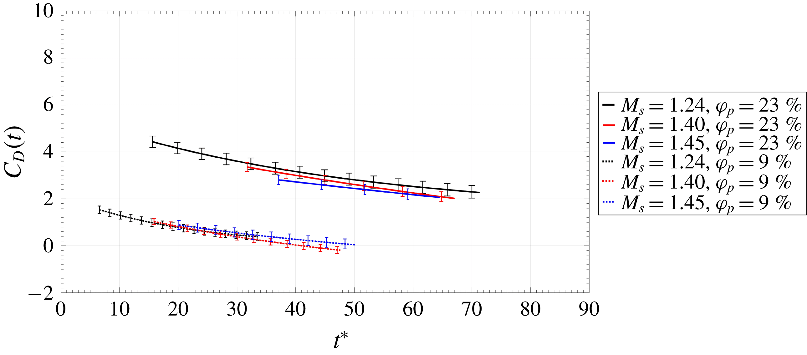
On the other hand, for a given particle curtain, Ling et al. (Reference Ling, Wagner, Beresh, Kearney and Balachandar2012) showed the spreading to collapse with a simpler non-dimensional time, namely a time scale representing the propagation time across the initial thickness of the curtain. More recently, work by DeMauro et al. (Reference DeMauro, Wagner, Beresh and Farias2017) used time-resolved particle image velocimetry to estimate the unsteady drag imposed on dense particle curtains. In these measurements, the pressure difference across the curtain was found to be the dominant contributor to drag, a sentiment echoed by the scaling arguments in Theofanous et al. (Reference Theofanous, Mitkin and Chang2016). Additionally, DeMauro et al. (Reference DeMauro, Wagner, Beresh and Farias2017) showed the drag to be a function of volume fraction, in agreement with the findings of Sen et al. (Reference Sen, Gaul, Choi, Jacobs and Udaykumar2017). These data are shown in figure 1, for two different volume fractions and three Mach numbers. Here,
 $C_{D}$
is defined as
 $$\begin{eqnarray}C_{D}(t)=\frac{2D(t)}{\unicode[STIX]{x1D70C}_{ind}U_{ind}^{2}A_{x}},\end{eqnarray}$$
where
 $A_{x}$
is the frontal area of the curtain,
 $D$
is the particle curtain drag, and
 $\unicode[STIX]{x1D70C}_{ind}$
and
 $U_{ind}$
are the induced density and velocity, respectively. In this sense, induced refers to the post-shock values these parameters take following the passage of the initial shock. In addition to this, time was non-dimensionalized in the same manner as Ling et al. (Reference Ling, Wagner, Beresh, Kearney and Balachandar2012) according to
 $$\begin{eqnarray}t^{\ast }=\frac{t}{\unicode[STIX]{x1D70F}}=\frac{U_{ind}}{\unicode[STIX]{x1D6FF}_{0}}t,\end{eqnarray}$$
where
 $\unicode[STIX]{x1D6FF}_{0}$
refers to the initial thickness of the particle curtain at mid-span.
Drag coefficient versus non-dimensional time, after DeMauro et al. (Reference DeMauro, Wagner, Beresh and Farias2017).

Following from this result and the work of DeMauro et al. (Reference DeMauro, Wagner, Beresh and Farias2017), the purpose of this paper is to perform a parametric study to experimentally investigate the influence of volume fraction, particle size, curtain thickness and shock strength on the spreading rate of the particle curtain. It was shown in that work that the pressure difference across the curtain was proportional to the volume fraction, motivating further exploration. Experimental data, obtained using high-speed schlieren imaging, is compared against published results from Wagner et al. (Reference Wagner, Beresh, Kearney, Trott, Castaneda, Pruett and Baer2012), Ling et al. (Reference Ling, Wagner, Beresh, Kearney and Balachandar2012), and Theofanous et al. (Reference Theofanous, Mitkin and Chang2016), allowing for comparison across a range of conditions. A new method of scaling time is proposed, which better collapses data of varying volume fraction. By performing this new scaling, the influence of the curtain volume fraction is emphasized, providing a more complete collapse. Other features that become apparent include the divergence observed in data sets associated with volume fractions either outside of the dense regime, or closer to the dilute regime.
2 Experimental setup
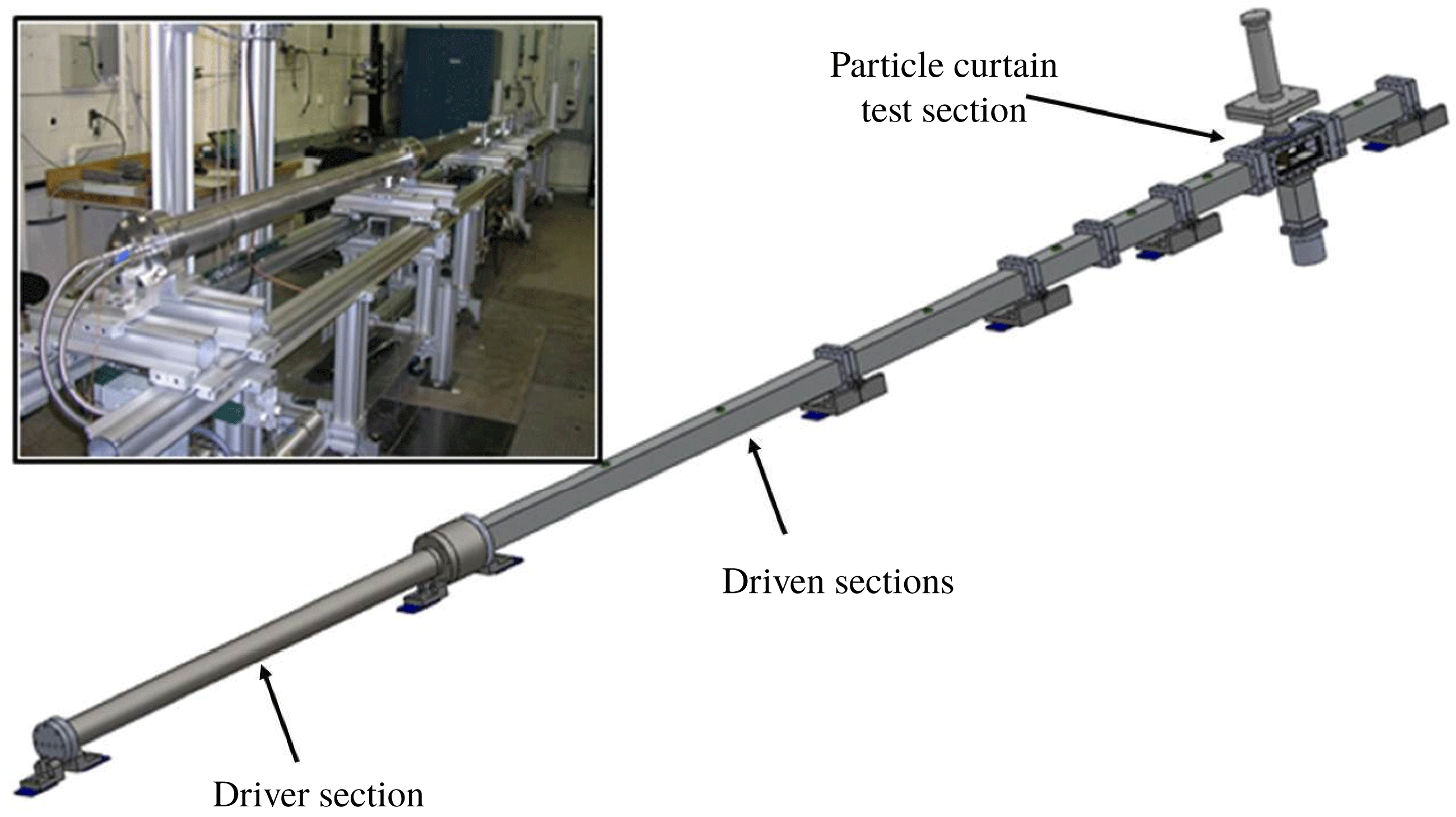
The multiphase shock tube (MST) is shown in figure 2. The driver section of the shock tube was constructed from a 2.1 m long stainless steel pipe with an inner diameter of 89 mm and a wall thickness of 12.7 mm, supplied with a high pressure nitrogen source. The driven section consists of square tubing, 5.2 m long, with an inner width of 76 mm and wall thickness of 12.7 mm. The driven gas was air at an initial temperature and absolute pressure of 297 K and 84.1 kPa, respectively. In lieu of burst discs, a Dynamics Systems Research (Model 183-1.5-2000) fast acting valve was used to fire the shock tube due to its repeatability and comparably rapid turnaround time. The valve has been shown to achieve a comparable flow quality to that obtained from a burst disc (Wagner et al. Reference Wagner, DeMauro, Casper, Beresh, Lynch and Pruett2018).
The MST with relevant sections identified.

Experiments were conducted at three shock Mach numbers:
 $M_{s}=1.24$
, 1.40, and 1.45, which corresponded to driver pressures of 690, 2070, and 2760 kPa. Prior to an experiment, soda lime particles rested on an initially closed gate valve. When the gate valve was opened, particles flowed through a bevelled slit in the test section ceiling under the influence of gravity, forming a particle curtain. The slit width was 3.2 mm and the curtain spanned the width of the test section unlike in Wagner et al. (Reference Wagner, Beresh, Kearney, Trott, Castaneda, Pruett and Baer2012, Reference Wagner, Kearney, Beresh, DeMauro and Pruett2015) and Ling et al. (Reference Ling, Wagner, Beresh, Kearney and Balachandar2012) where the curtain spanned 88 % of the test section width. Experiments with the slits, but without the particle curtain, have revealed the overall effect on the shock is minimal as the shock-induced pressure upstream and downstream of the slits is identical within measurement uncertainty. The particle curtain was allowed to flow through the test section for 1 s in order to ensure that steady state had been reached within the curtain (note that steady state was obtained after 50 ms) before the shock tube was fired. The particles exited the test section through a similar slit in the floor, where they entered a collection reservoir.
As described in DeMauro et al. (Reference DeMauro, Wagner, Beresh and Farias2017), an extensive set of tests were conducted to characterize and quantify the particle curtain, including measurements of the particle velocity, mass flow rate, and curtain thickness. As the particles free-fall from the open slit, their velocity increases under the influence of gravity; i.e.
 $u_{p}(y)\approx \sqrt{2g(y+H/2)}$
, where
 $g$
is the acceleration due to gravity and
 $H$
is the height of the shock tube. Assuming a constant cross-sectional area,
 $A_{c}$
, the density of the particle curtain, as a function of height, can be shown to be
 $$\begin{eqnarray}\unicode[STIX]{x1D70C}_{mix}(y)=\frac{{\dot{m}}_{mix}}{u_{p}(y)A_{c}},\end{eqnarray}$$
where
 $u_{p}$
is the velocity of the particles. The particles were observed to free-fall at a velocity of
 $0.89~\text{m}~\text{s}^{-1}$
at approximately mid-height; therefore they were essentially frozen in comparison to the shock velocities. Because the volume fraction varies across the height of the particle curtain, the volume fraction (
 $\unicode[STIX]{x1D711}_{p}$
) reported in this study corresponded to that measured at mid-height, determined from
 $$\begin{eqnarray}\unicode[STIX]{x1D711}_{p}=\frac{\forall _{p}}{\forall _{mix}}=\frac{\unicode[STIX]{x1D70C}_{mix}-\unicode[STIX]{x1D70C}_{air}}{\unicode[STIX]{x1D70C}_{p}-\unicode[STIX]{x1D70C}_{air}},\end{eqnarray}$$
where
 $\unicode[STIX]{x1D70C}_{mix}$
is the density of the total mixture,
 $\unicode[STIX]{x1D70C}_{air}$
is the density of air, and
 $\unicode[STIX]{x1D70C}_{p}$
is the density of the particles.
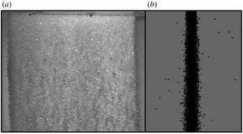
Instantaneous image of the particle curtain obtained at an oblique angle (a); instantaneous side-view of the particle curtain used to measure the curtain thickness (b). Note that a background subtraction has been performed in both images in order to highlight the relevant features.

Particle curtain data.

a From Wagner et al. (Reference Wagner, Beresh, Kearney, Trott, Castaneda, Pruett and Baer2012, Reference Wagner, Kearney, Beresh, DeMauro and Pruett2015) and Ling et al. (Reference Ling, Wagner, Beresh, Kearney and Balachandar2012).
b From Theofanous et al. (Reference Theofanous, Mitkin and Chang2016).
Figure 3 shows the particle curtain, acquired at an oblique angle, along with a back-lit image of the curtain used to measure the curtain thickness. Table 1 shows the volume fractions of the conducted tests, corresponding to the assumption of a uniform particle distribution. For experiments conducted at Sandia, the particles were thoroughly sieved but still retain a distribution of particle diameters, which are specified in table 1 for each of the experiments. In addition, sieved particles were visually inspected by microscope to ensure that the vast majority of them were spherical or nearly so. Note that in reality, the curtain has a streamwise Gaussian particle distribution (Regele et al. Reference Regele, Rabinovitch, Colonius and Blanquart2014; Goetsch & Regele Reference Goetsch and Regele2015; Wagner et al. Reference Wagner, Kearney, Beresh, DeMauro and Pruett2015); however, for purposes of simplicity, distribution is neglected here. In other words, a top-hat (constant volume fraction) is assumed. As is evident, the data summarized in table 1 represents a variety of particle sizes, volume fractions, curtain thicknesses, and a wide range of shock Mach numbers. These data have been collected from the published results of Ling et al. (Reference Ling, Wagner, Beresh, Kearney and Balachandar2012) and Theofanous et al. (Reference Theofanous, Mitkin and Chang2016), along with newer results obtained for this study. To the authors’ knowledge, the experiments listed in table 1 represent all of the particle curtain interaction data in the dense volume fraction regime.
Schlieren imaging was performed to visualize the direct interaction of the shock wave with the particle curtain, along with the resulting relevant flow features. The light source was a Visual Instrumentation Corporation continuous-wave high brightness light emitting diode (Model 900415). Two 101.6 mm plano-convex lenses both with a focal length of 463.5 mm were used; the first to collimate the light before entry into the test section and the secondary plano-convex lens to focus the light exiting the test section onto a vertical knife-edge. Images were acquired using a Photron SA-Z camera at a resolution of
 $680\times 340$
pixels, operating at a framing rate of 75 kHz.
For the data obtained at Sandia, quantification of the curtain spreading was performed using the instantaneous schlieren images. The edges of the curtain were defined according to the same method in Ling et al. (Reference Ling, Wagner, Beresh, Kearney and Balachandar2012), where the upstream/downstream edges were taken at 95 % of the curtain’s maximum pixel intensity. This is similar to the previous studies (Ling et al.
Reference Ling, Wagner, Beresh, Kearney and Balachandar2012; Wagner et al.
Reference Wagner, Beresh, Kearney, Trott, Castaneda, Pruett and Baer2012, Reference Wagner, Kearney, Beresh, DeMauro and Pruett2015), where the edge positions were found at the location corresponding to the vertical centre of the curtain. For the
 $\unicode[STIX]{x1D711}_{p}=$
9 % case, it should be noted that there are relatively fewer particles across the thickness of the curtain compared to other cases. Lv et al. (Reference Lv, Wang, Zhang and Li2018) mentions that the skeleton of the curtain, is the dominant metric compared to the actual thickness of the curtain. This is noted in their emphasis on the metric comprising the volume fraction, multiplied by the initial curtain thickness, as opposed to the total number of particles. Pinker & Herbert (Reference Pinker and Herbert1967) support this notion in their manner of defining screen drag porosity. Finally, it should be pointed out that this curtain still behaves in a similar way to the higher volume fractions, as will be shown subsequently.
3 Results/discussion
3.1 Physical description of curtain interaction
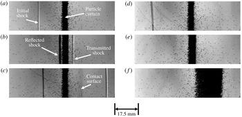
Prior to discussion of induced particle curtain spreading, it is important to first illustrate the essential physics of the interaction. Figure 4 shows a sample set of schlieren images associated with an
 $M_{s}=1.40$
shock wave interaction with a particle curtain composed of
 $d_{p}=300{-}355~\unicode[STIX]{x03BC}\text{m}$
, issuing from a 3.2 mm slit. The time steps are used to identify key features associated with this motion. Note that time has been defined such that
 $t=0~\text{s}$
corresponds to the instant the initial shock wave reaches the particle curtain.
The initial shock propagating towards the upstream edge of the particle curtain is shown in figure 4(a). Following interaction, a reflected shock wave is created, which moves back upstream, while a transmitted shock wave can be seen moving downstream of the curtain (figure 4 b). The relative strengths of these two shock waves correspond to the volume fraction of the curtain (DeMauro et al. Reference DeMauro, Wagner, Beresh and Farias2017). In this case, the transmitted shock wave is much faster than the reflected one, and a favourable pressure gradient is set up across the particle curtain. Figure 4(c) also highlights the presence of a contact surface between the particle curtain and the transmitted shock (Ling et al. Reference Ling, Wagner, Beresh, Kearney and Balachandar2012).
The transmitted shock wave has propagated outside of the field of view in figure 4(d), and by figure 4(e), the reflected shock wave has also left the field of view. The pressure gradient imposed on the curtain begins to cause the curtain to deform and spread as it moves downstream (figure 4 e,f). An interesting observation here is the apparent time lag associated with deformation of the particle curtain. The curtain was not seen to move until some time after interaction with the initial shock wave and the passage of the secondary shock waves, which has not been previously noted experimentally within the literature; however, a similar observation was made within the theoretical work of Kosinski (Reference Kosinski2008). Similarly, this can also be seen within figure 9(b) of Theofanous, Mitkin & Chang (Reference Theofanous, Mitkin and Chang2018), although it was unrecognized.
Schlieren imaging of the
 $M_{s}=1.40$
shock wave interaction with the
 $d_{p}=300{-}355~\unicode[STIX]{x03BC}\text{m}$
particle curtain:
 $t^{\ast }=$
(a)
 $-2.27$
; (b) 0.76; (c) 3.78; (d) 6.80; (e) 12.85; (f) 43.08.

The spreading rate was measured for each of the conditions shown in table 1, beginning at
 $t=0~\text{s}$
, by recording the position of the upstream and downstream edges of the curtain at mid-height. These data are shown in figure 5. The upstream edge is defined as being initially at
 $x=0~\text{mm}$
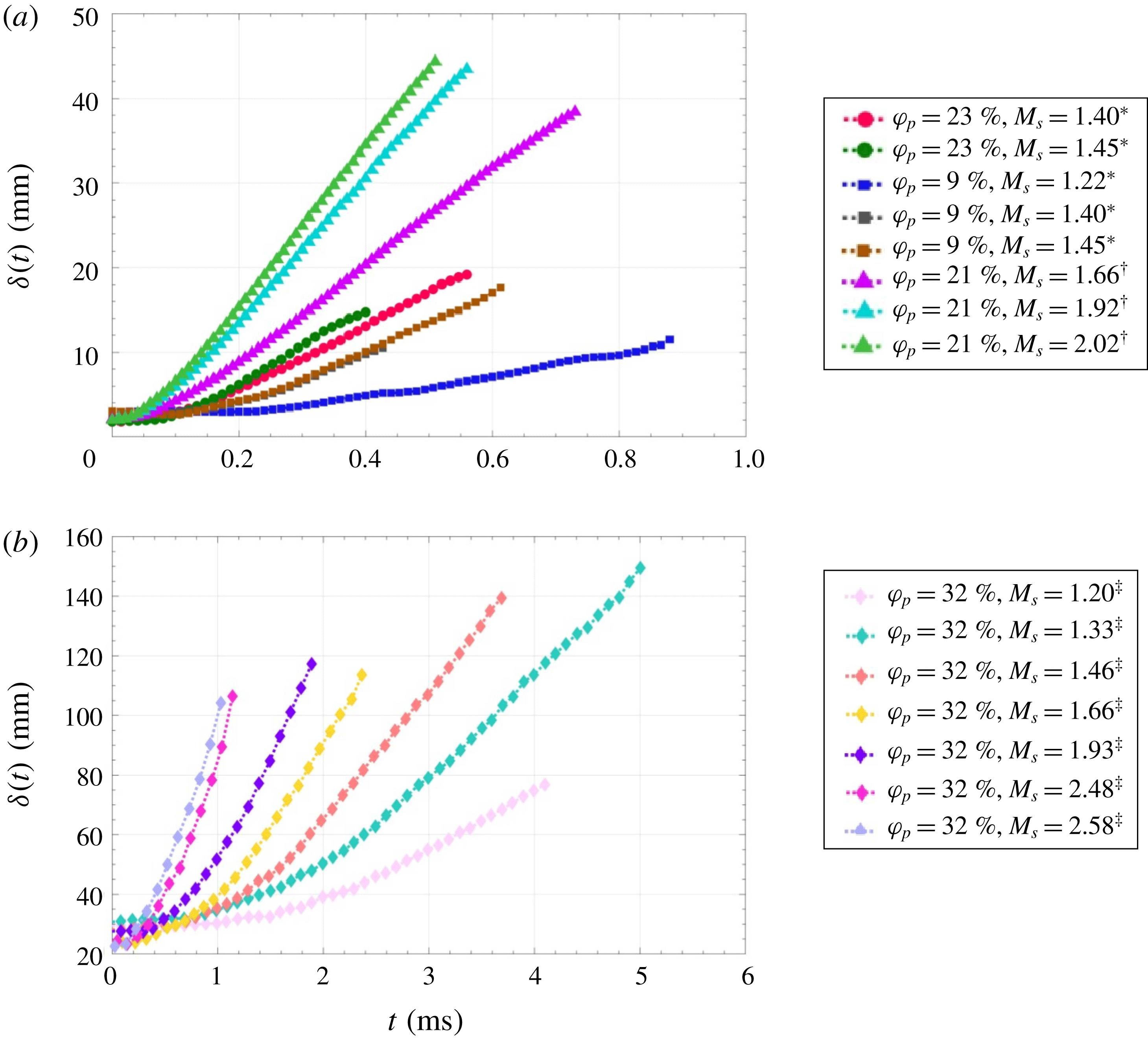
. As is evident from the trends shown in figure 5, the data behave similarly; i.e. a relatively constant region appears at early times following the interaction with the shock wave, followed by a curved region constant acceleration region and then a linear constant velocity region (Theofanous et al.
Reference Theofanous, Mitkin and Chang2016). However, the spreading of the curtain is observed to be a function of both the Mach number of the initial shock and the volume fraction of the curtain.
Spreading of the curtains described in table 1, as a function of time: (a) data from MST; (b) data from Theofanous et al. (Reference Theofanous, Mitkin and Chang2016).

3.2 Scaling of the particle curtain spreading
3.2.1 Scaling based on convective time scale
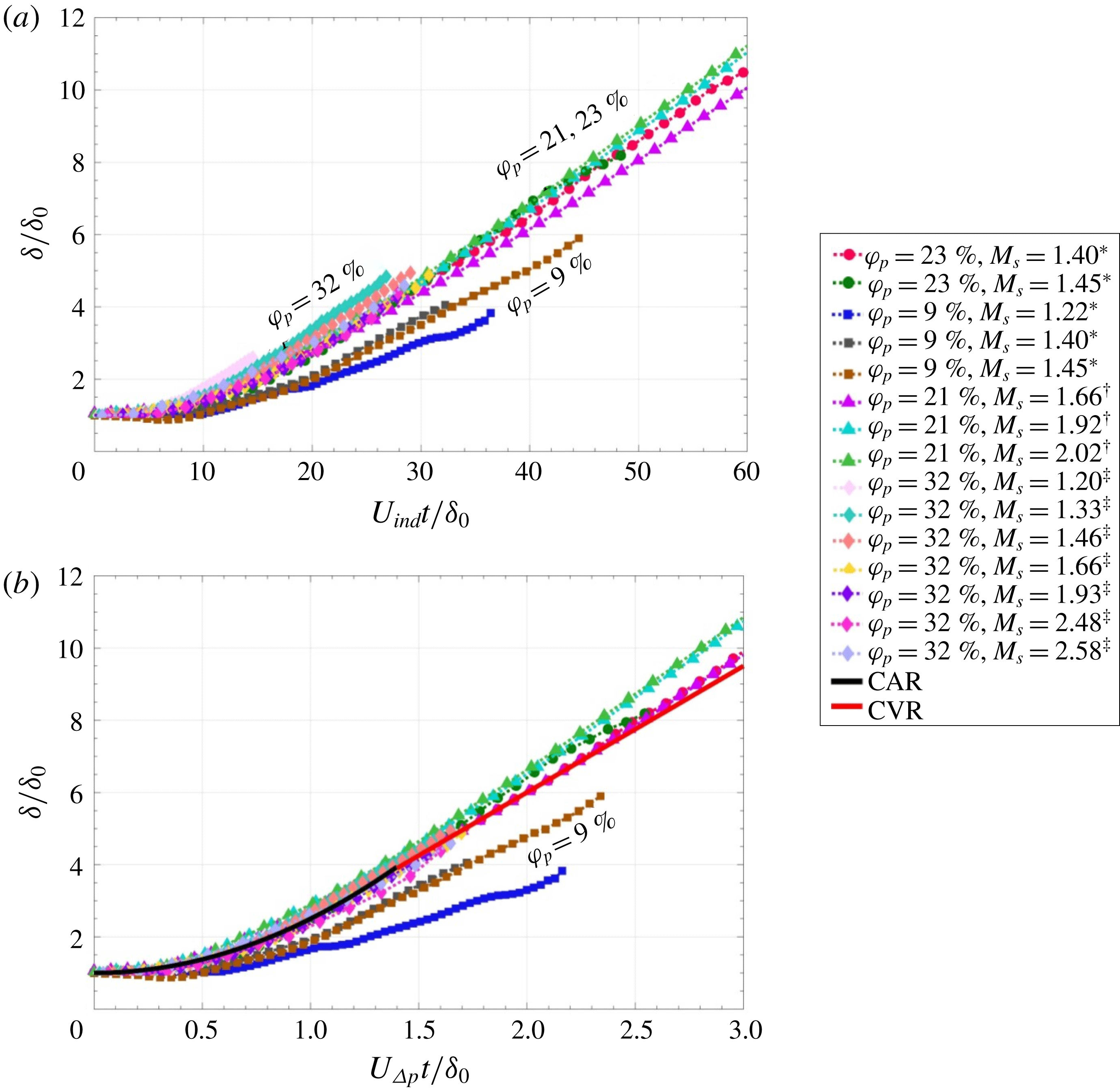
As was seen in figure 1, scaling of the estimated curtain drag by conditions following the passage of the initial shock wave resulted in a collapse of the drag data into two regions based on volume fraction. As the spreading of the curtain is a direct result of the imposed drag, such a separation should be clearly evident in the spreading rate also. The spreading rates of the curtains are shown in figure 6, where in figure 6(a) time is scaled according to the definition given in (1.2), whereas figure 6(b) shows the same data, with time scaled as suggested by Theofanous et al. (Reference Theofanous, Mitkin and Chang2016)
 $$\begin{eqnarray}t_{t}^{\ast }=\frac{t}{\unicode[STIX]{x1D70F}_{t}}=\frac{t}{\unicode[STIX]{x1D6FF}_{0}}\sqrt{\left(\frac{P_{1}}{\unicode[STIX]{x1D70C}_{p}}\right)\left(\frac{P_{wall}}{P_{1}}-1\right)}=\frac{U_{\unicode[STIX]{x0394}P}}{\unicode[STIX]{x1D6FF}_{0}}t,\end{eqnarray}$$
where
 $P_{wall}$
is the pressure following the passage of a shock wave reflected off a hypothetical wall at the location of the particle curtain. From this definition, it is apparent that (3.1) is a time scale based on a modified particle propagation time; the new velocity,
 $U_{\unicode[STIX]{x0394}P}$
is associated with the reflected shock pressure, the initial pressure inside the shock tube (
 $P_{1}$
) and the density of the curtain particles,
 $\unicode[STIX]{x1D70C}_{p}$
.
Comparison of the non-dimensionalization methods of (a) Ling et al. (Reference Ling, Wagner, Beresh, Kearney and Balachandar2012) and (b) Theofanous et al. (Reference Theofanous, Mitkin and Chang2016). The data associated with
 $\unicode[STIX]{x1D711}_{p}=32\,\%$
was taken from Theofanous et al. (Reference Theofanous, Mitkin and Chang2016).

Both scaling methods appear to provide varying degrees of success with regards to collapse of the data. In each case, curves associated with
 $\unicode[STIX]{x1D711}_{p}=9\,\%$
appear to diverge from the general trend of the other curves. As the particle curtain deforms, the 9 % volume fraction curves deviate from the general trend, which may be a consequence of volume fraction.
In figure 6(a), non-dimensionalization of time by (1.2) results in the data of Theofanous et al. (Reference Theofanous, Mitkin and Chang2016) slightly overshooting the general trend of the collapsed data. This is corrected, however, in figure 6(b), where all data (with the exception of that corresponding to
 $\unicode[STIX]{x1D711}_{p}=9\,\%$
) shows a much improved collapse. Included in figure 6(b) are the empirical lines corresponding to the Constant Acceleration Regime (CAR) and Constant Velocity Regime (CVR); these are given by
 $$\begin{eqnarray}\displaystyle & \displaystyle \unicode[STIX]{x1D6FF}\sim 1+1.5\left(\frac{U_{\unicode[STIX]{x0394}P}}{\unicode[STIX]{x1D6FF}_{0}}t\right)^{2} & \displaystyle\end{eqnarray}$$
 $$\begin{eqnarray}\displaystyle & \displaystyle \unicode[STIX]{x1D6FF}\sim 2.5+3.5\left(\frac{U_{\unicode[STIX]{x0394}P}}{\unicode[STIX]{x1D6FF}_{0}}t-1\right), & \displaystyle\end{eqnarray}$$
where (3.2) is defined for
 $t_{t}^{\ast }<1.4$
, and (3.3) for
 $t_{t}^{\ast }>1$
(Theofanous et al.
Reference Theofanous, Mitkin and Chang2016). In general, equations (3.2) and (3.3) do well at modelling the trends associated with
 $\unicode[STIX]{x1D711}_{p}=21$
, 23 and 32 % for
 $t_{t}^{\ast }<1.5$
, but fail to capture the trends for the lower volume fractions. Therefore, these laws appear to best describe trends associated with dense curtains of sufficiently high volume fractions only. In addition, both the CAR and CVR curves under-predict the long term trends in the higher
 $\unicode[STIX]{x1D711}_{p}$
data for
 $t_{t}^{\ast }>1.5$
.
At early time,
 $t_{t}^{\ast }<0.3$
, a nearly constant curtain thickness universally exists, implying that the curtain has a time lag between shock wave interaction and the beginning of deformation. Within the CAR, an acceleration is imposed on the particle curtain, associated with the formation of the reflected and transmitted shock waves, and the initial response of the curtain to these imposed forces. Much of this CAR behaviour may be restricted to the establishment of the flows upstream/downstream of the curtain. On the other hand, the drag data shown in figure 1 appears to correspond to the CVR; therefore, the CVR corresponds to the times where the flow conditions on either side of the curtain begin to equilibrate.
3.2.2 Incorporation of
 $\unicode[STIX]{x1D711}_{p}$

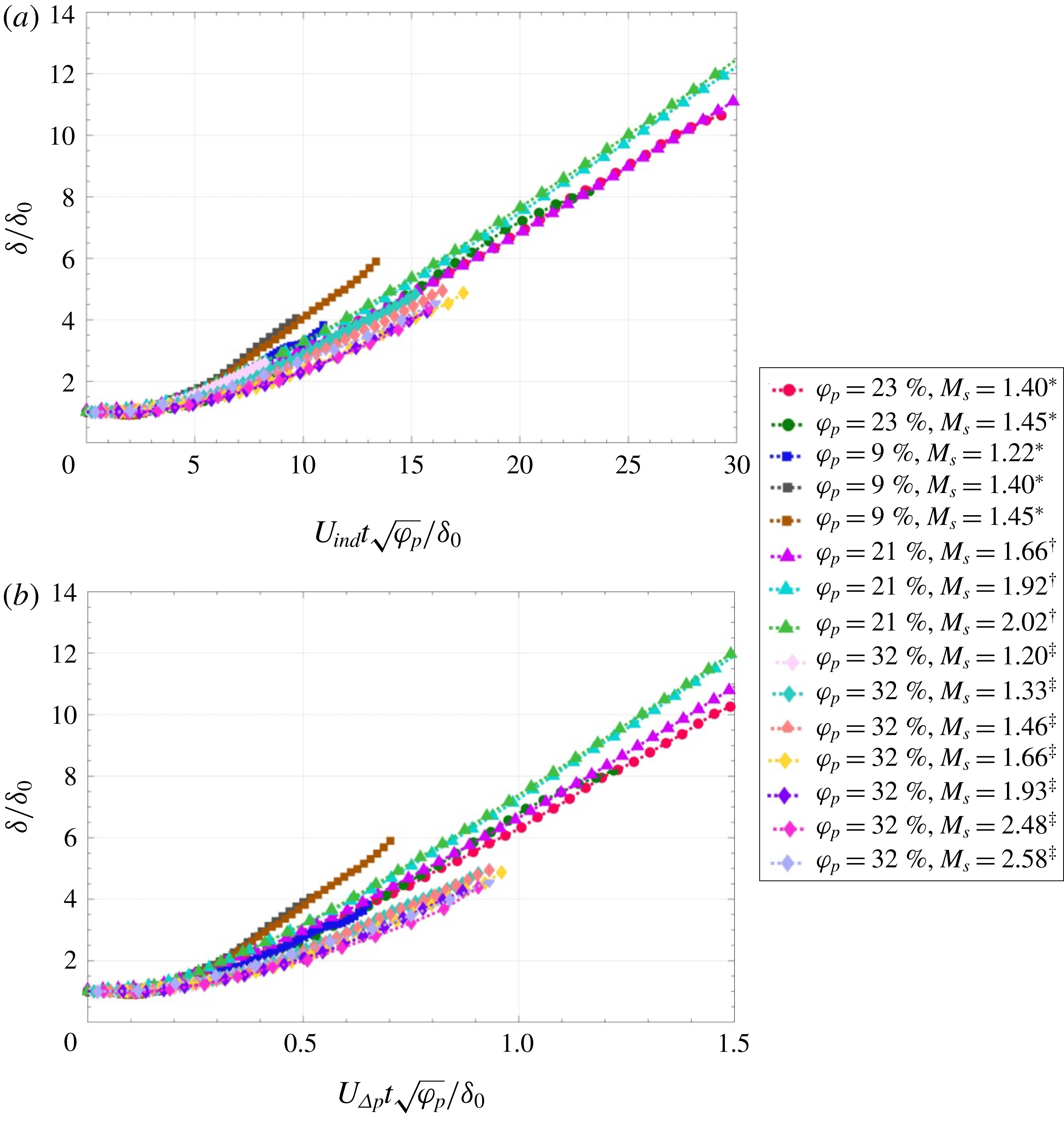
It is obvious from figure 6 that the time scale requires information regarding the volume fraction of the particle curtain in order to negotiate collapse of the disparate volume fractions. Figure 7 attempts to incorporate volume fraction into the determination of the time scale by multiplying each non-dimensional time by
 $\sqrt{\unicode[STIX]{x1D711}_{p}}$
. The motivation for such a multiplier was to take the time scale defined in (3.1) and scale the
 $P_{wall}$
term by the volume fraction of the particle curtain to approximate the effects of porosity.
Modification of the non-dimensionalization methods of (a) Ling et al. (Reference Ling, Wagner, Beresh, Kearney and Balachandar2012) and (b) Theofanous et al. (Reference Theofanous, Mitkin and Chang2016) by multiplying non-dimensional time by
 $\sqrt{\unicode[STIX]{x1D711}_{p}}$
.

Comparing figure 7(a) to 7(b), it is apparent that a more complete collapse of the data is obtained in figure 7(a), where the multiplying factor of
 $\sqrt{\unicode[STIX]{x1D711}_{p}}$
was applied to the time scale defined by (1.2). Specifically, the major difference between the two methods involves the use of a modified form of the scaling of Ling et al. (Reference Ling, Wagner, Beresh, Kearney and Balachandar2012) in figure 7(a) compared to a modification to the scaling of Theofanous et al. (Reference Theofanous, Mitkin and Chang2016) in figure 7(b). Here, the
 $\unicode[STIX]{x1D711}_{p}=9\,\%$
data appears to diverge at earlier times compared to the higher
 $\unicode[STIX]{x1D711}_{p}$
curves. In contrast, applying the multiplier to figure 7(b) resulted in an improved collapse of the data compared to figure 6(b), although not as well as figure 7(a). In both cases, similar regimes identified for figure 6(b) remain; namely a time lag associated with spreading of the particle curtain, a CAR and a CVR.
The choice in using
 $\sqrt{\unicode[STIX]{x1D711}_{p}}$
was based on the assumption that pressure-differential is directly proportional to the volume fraction. With this method, an apparent improvement in the collapse is indeed observed. As an alternative, a simplified force balance was used to relate the curtain spreading to incompressible drag through a grid. This force balance takes the form of
 $$\begin{eqnarray}\unicode[STIX]{x1D711}_{p}\unicode[STIX]{x1D70C}_{p}A_{x}\unicode[STIX]{x1D6FF}_{0}\frac{\text{d}^{2}x}{\text{d}t^{2}}=\frac{1}{2}C_{D}\unicode[STIX]{x1D70C}_{ind}\left(U_{ind}-\frac{\text{d}x}{\text{d}t}\right)^{2}A_{x}.\end{eqnarray}$$
Notice that the particle curtain is treated as an equivalent semi-permeable body with an associated drag. Moreover, the drag force term on the right-hand side is modelled in terms of the imposed relative velocity. While (3.4) is separable and readily integrated, the resulting expression does not exhibit the simple analytical form that is of use to identify scaling behaviour. As such, a modification of the formulation is introduced, whereby the behaviour of the relative velocity is ignored and the density is modelled using the pre-shock gas density instead,
 $\unicode[STIX]{x1D70C}_{1}$
. The effect of these two approximations will then cancel each other in the right-hand side of (3.4) while yielding a simple analytical solution. Note that Theofanous et al. (Reference Theofanous, Mitkin and Chang2016) also suggest the use of initial conditions in the driven gas in their scaling arguments. This results in the approximation of the form
 $$\begin{eqnarray}\unicode[STIX]{x1D711}_{p}\unicode[STIX]{x1D70C}_{p}\unicode[STIX]{x1D6FF}_{0}\frac{\text{d}^{2}x}{\text{d}t^{2}}=\frac{1}{2}C_{D}\unicode[STIX]{x1D70C}_{1}U_{ind}^{2}.\end{eqnarray}$$
Integration produces
 $$\begin{eqnarray}\frac{x}{\unicode[STIX]{x1D6FF}_{0}}=\frac{1}{4}\frac{C_{D}}{\unicode[STIX]{x1D711}_{p}}\left(\frac{\unicode[STIX]{x1D70C}_{1}}{\unicode[STIX]{x1D70C}_{p}}\right)\left(\frac{U_{ind}t}{\unicode[STIX]{x1D6FF}_{0}}\right)^{2}.\end{eqnarray}$$
To proceed with (3.6), a model for the drag is needed. For this analysis, the drag coefficient will be modelled by analogy with pressure drop over porous screens. It was previously shown by DeMauro et al. (Reference DeMauro, Wagner, Beresh and Farias2017) that such a pressure drop is dependent on the volume fraction. Though the rigidity of a grid is physically inaccurate, this is a useful mathematical simplification to reach a new scaling law formulation. Following Pinker & Herbert (Reference Pinker and Herbert1967), the expressions are of the form
 $$\begin{eqnarray}C_{D}\propto \frac{\unicode[STIX]{x1D711}_{p}^{\unicode[STIX]{x1D6FC}}}{(1-\unicode[STIX]{x1D711}_{p})^{2}},\end{eqnarray}$$
where
 $1<\unicode[STIX]{x1D6FC}<2$
are shown to be effective for a range of screen pressure drop problems. A simplification to approximately honour these two limits is to take a geometric average of the drag expressions as
 $$\begin{eqnarray}C_{D}\propto \sqrt{\left[\frac{\unicode[STIX]{x1D711}_{p}}{(1-\unicode[STIX]{x1D711}_{p})^{2}}\right]\left[\frac{\unicode[STIX]{x1D711}_{p}^{2}}{(1-\unicode[STIX]{x1D711}_{p})^{2}}\right]}=\frac{\unicode[STIX]{x1D711}_{p}^{3/2}}{(1-\unicode[STIX]{x1D711}_{p})^{2}}.\end{eqnarray}$$
 $$\begin{eqnarray}\frac{x}{\unicode[STIX]{x1D6FF}_{0}}=\frac{1}{4}\frac{C_{D}}{\unicode[STIX]{x1D711}_{p}}\frac{\unicode[STIX]{x1D711}_{p}^{3/2}}{(1-\unicode[STIX]{x1D711}_{p})^{2}}\left(\frac{\unicode[STIX]{x1D70C}_{1}}{\unicode[STIX]{x1D70C}_{p}}\right)\left(\frac{U_{ind}t}{\unicode[STIX]{x1D6FF}_{0}}\right)^{2}=\frac{1}{4}C_{D_{0}}\frac{\unicode[STIX]{x1D711}_{p}^{1/2}}{(1-\unicode[STIX]{x1D711}_{p})^{2}}\left(\frac{U_{ind}t}{\unicode[STIX]{x1D6FF}_{0}}\right)^{2}.\end{eqnarray}$$
where
 $C_{D_{0}}$
is a remaining constant of proportionality. An expansion of the volume fraction term can be performed, according to
 $$\begin{eqnarray}\frac{\unicode[STIX]{x1D711}_{p}^{1/2}}{(1-\unicode[STIX]{x1D711}_{p})^{2}}=\unicode[STIX]{x1D711}_{p}^{1/2}+\cdots \mathit{O}(\unicode[STIX]{x1D711}_{p}^{3/2}).\end{eqnarray}$$
Applying this expansion then results in
 $$\begin{eqnarray}\frac{x}{\unicode[STIX]{x1D6FF}_{0}}\propto \left(\unicode[STIX]{x1D711}_{p}^{1/4}\frac{U_{ind}t}{\unicode[STIX]{x1D6FF}_{0}}\right)^{2}.\end{eqnarray}$$
Equation (3.11) therefore suggests that the scaling argument should be proportional to
 $\unicode[STIX]{x1D711}_{p}^{1/4}$
for the particle trajectory. It should be noted that the application of this scaling method made use strictly of a screen-drag argument, which is based on area-blockage. In this sense, a thin curtain behaves similarly to a thin screen.
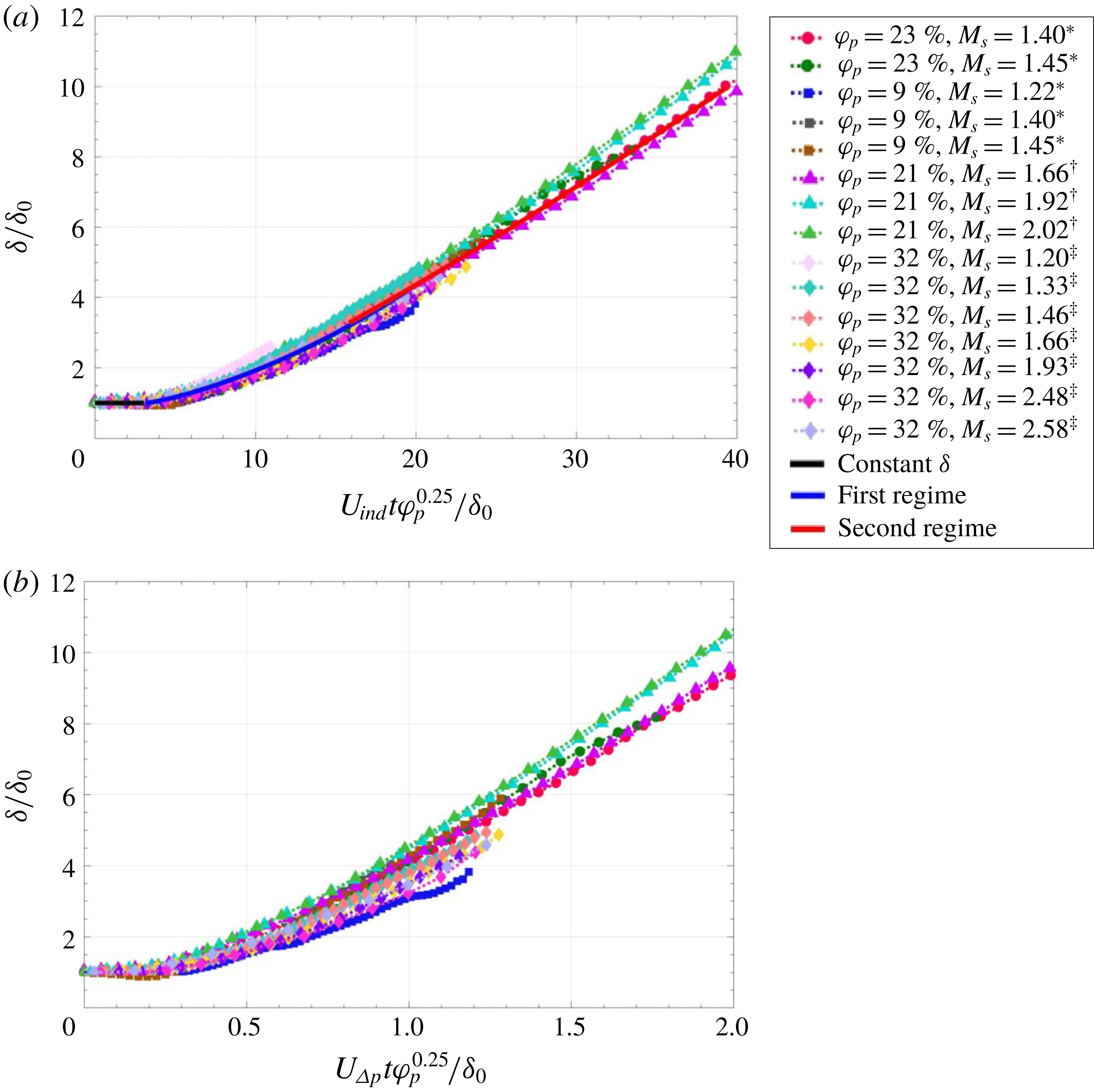
Application of (3.11) to the curtain spreading data is shown in figure 8. Indeed, an improved collapse is observed in figure 8 compared to figure 7, which brings even the
 $\unicode[STIX]{x1D711}_{p}=9\,\%$
data into agreement with the higher volume fraction data. Comparing between the time scale found using (3.1) and (1.2), a more complete collapse of the data is obtained by applying this multiplier to the latter, whereas figure 8(b) continues to show discrepancies associated with the lower volume fraction. These findings agree well with the previous argument that the multiplier in (3.11) should function best when applied to the non-dimensionalization of time using (1.2).
Comparison of the non-dimensionalization methods of (a) Ling et al. (Reference Ling, Wagner, Beresh, Kearney and Balachandar2012) and (b) Theofanous et al. (Reference Theofanous, Mitkin and Chang2016). The data associated with
 $\unicode[STIX]{x1D711}_{p}=32\,\%$
was taken from Theofanous et al. (Reference Theofanous, Mitkin and Chang2016). Modification performed by multiplying time scale by
 $\unicode[STIX]{x1D711}_{p}^{0.25}$
.

In general, the data shown here illustrate that a need for incorporation of a function of the volume fraction into the characteristic time scale is required for complete collapse of the spreading data. Such discrepancies were observed in figure 1; furthermore, while use of (3.1) and (1.2) saw improved collapse of the particle curtain spreading data, this was only seen to occur as long as the data to be collapsed were of a similar volume fraction. Smaller volume fractions transition more rapidly into the dilute mixture regime, where agreement begins to suffer. For completeness, the present results were compared to the granular (
 $\unicode[STIX]{x1D711}_{p}=64\,\%$
) experiments of Rogue et al. (Reference Rogue, Rodriguez, Haas and Saurel1998) and to the dilute data (
 $\unicode[STIX]{x1D711}_{p}=\sim 1\,\%$
) of Theofanous et al. (Reference Theofanous, Mitkin and Chang2018). The scaling proposed here was found to over-predict the spread of the dilute data of (Theofanous et al.
Reference Theofanous, Mitkin and Chang2018) and under-predict the granular results of Rogue et al. (Reference Rogue, Rodriguez, Haas and Saurel1998). This indicates that the proposed scaling is applicable at dense volume fractions, but not in the dilute or granular regimes.
In addition, figure 8(a) is superimposed with functions modelling portions of the spreading rate. These functions were determined from observing a log–log plot of the data and subdividing based on changes in curvature. To this end, the first regime is a constant curtain thickness regime, where no change was observed with time. Following this, two trends were noted. Within the range of
 $3.16\leqslant t^{\ast }\leqslant 19.95$
(
 $R^{2}=0.96$
)
 $$\begin{eqnarray}\log _{10}\left(\frac{\unicode[STIX]{x1D6FF}}{\unicode[STIX]{x1D6FF}_{0}}\right)=0.758(\log _{10}t^{\ast })^{2}-0.57\log _{10}t^{\ast }+0.09.\end{eqnarray}$$
Within the range of
 $10\leqslant t^{\ast }\leqslant 40$
(
 $R^{2}=0.99$
)
 $$\begin{eqnarray}\log _{10}\left(\frac{\unicode[STIX]{x1D6FF}}{\unicode[STIX]{x1D6FF}_{0}}\right)=1.22\log _{10}t^{\ast }-0.95.\end{eqnarray}$$
Equations (3.12) and (3.13) show that the data assumes a quadratic and linear distribution when observed in a log–log format. As can be seen from figure 8, these trends appear to hold well for all the data and may be useful for estimation of a curtain spreading rate. Note that, in effect, the motion is delayed in time to accommodate the constant-thickness time span mentioned previously.
4 Conclusions
Experiments were conducted in Sandia’s multiphase shock tube facility using high-speed schlieren imaging to quantify the deformation of a dense gas–solid mixture following interaction with a shock wave. The mixture was in the form of a particle curtain, which was a thin two-dimensional obstruction to the streamwise flow within the shock tube. Previous measurements of the unsteady drag imposed on the particle curtain showed that the resulting unsteady drag coefficient was dependent on volume fraction. Following from this finding, spreading rates for curtains across a variety of volume fractions were used to investigate new scaling methods incorporating volume fraction into non-dimensional time.
One new result is the identification of a constant-thickness regime within the data, illustrating a delay associated with the timing shock impingement on the particle curtain and the beginning of curtain spreading. Upon collapse of the data, this constant regime was noted to be a commonality across the entirety of the data set. Such a result has not been previously commented upon within the literature; however, the data presented here highlight that it exists across data sets collected by different researchers.
It was shown that non-dimensionalization of time based on the particle propagation time across the thickness of the curtain returned a partial collapse of the data, where discrepancies were associated with volume fractions. Following the method of Theofanous et al. (Reference Theofanous, Mitkin and Chang2016), these discrepancies remained.
Finally, a theoretical argument was put forward to approximate the spreading of the curtain as a function of time using a simplified force balance and by treating the particle curtain as a porous screen. This method produced a drag proportional to
 $\unicode[STIX]{x1D711}_{p}^{1/4}$
, providing a theoretical basis for its success in collapsing the spreading data.
Acknowledgements
This work is supported by Sandia National Laboratories and the United States Department of Energy. Sandia National Laboratories is a multi-mission laboratory managed and operated by National Technology and Engineering Solutions of Sandia, LLC, a wholly owned subsidiary of Honeywell International, Inc., for the US Department of Energy’s National Nuclear Security Administration under contract DE-NA0003525.