




No CrossRef data available.
Article contents
- Abstract
- 1. INTRODUCTION
- 2. ON AR(1) MODELS
- 3. PROFILE LIKELIHOOD ANALYSIS AND UNIT-ROOT ASYMPTOTICS FOR THE ARB(1) MODEL
- 4. ADJUSTED PROFILE LIKELIHOOD
- 5. ADJUSTED PROFILE LIKELIHOOD ANALYSIS AND UNIT-ROOT ASYMPTOTICS FOR THE ARB(1) MODEL
- 6. STATISTICS AND UNIT-ROOT ASYMPTOTICS FOR THE ARμ(1) MODEL
- 7. FRACTILES FOR THE UNIT-ROOT ARB(1) MODEL
- 8. FRACTILES FOR THE UNIT-ROOT ARμ(1) MODEL
- 9. COMPARING ESTIMATION ACCURACY
- 10. NEAR UNIT-ROOT ASYMPTOTICS UNDER THE ARB(1) MODEL
- 11. NEAR UNIT-ROOT ASYMPTOTICS UNDER THE ARμ(1) MODEL
- 12. UNIT-ROOT TESTS AND POWER COMPARISONS FOR THE ARB(1) MODEL
- 13. UNIT-ROOT TESTS AND POWER COMPARISONS FOR THE ARμ(1) MODEL
- 14. POWER COMPARISON BETWEEN THE TWO AR(1) MODELS
- 15. DISCUSSION
- APPENDIX A: NEAR UNIT-ROOT ASYMPTOTICS FOR THE ARB(1) MODEL
- APPENDIX B: NEAR UNIT-ROOT ASYMPTOTICS FOR THE ARμ(1) MODEL
- APPENDIX C: INVARIANCE AND SIMILARITY RESULTS FOR THE ARB(1) MODEL
- APPENDIX D: ON THE SIMULATIONS
- References
AR(1) MODELS, UNIT ROOTS, AND ADJUSTED PROFILE LIKELIHOOD
Published online by Cambridge University Press: 24 September 2003
Article contents
- Abstract
- 1. INTRODUCTION
- 2. ON AR(1) MODELS
- 3. PROFILE LIKELIHOOD ANALYSIS AND UNIT-ROOT ASYMPTOTICS FOR THE ARB(1) MODEL
- 4. ADJUSTED PROFILE LIKELIHOOD
- 5. ADJUSTED PROFILE LIKELIHOOD ANALYSIS AND UNIT-ROOT ASYMPTOTICS FOR THE ARB(1) MODEL
- 6. STATISTICS AND UNIT-ROOT ASYMPTOTICS FOR THE ARμ(1) MODEL
- 7. FRACTILES FOR THE UNIT-ROOT ARB(1) MODEL
- 8. FRACTILES FOR THE UNIT-ROOT ARμ(1) MODEL
- 9. COMPARING ESTIMATION ACCURACY
- 10. NEAR UNIT-ROOT ASYMPTOTICS UNDER THE ARB(1) MODEL
- 11. NEAR UNIT-ROOT ASYMPTOTICS UNDER THE ARμ(1) MODEL
- 12. UNIT-ROOT TESTS AND POWER COMPARISONS FOR THE ARB(1) MODEL
- 13. UNIT-ROOT TESTS AND POWER COMPARISONS FOR THE ARμ(1) MODEL
- 14. POWER COMPARISON BETWEEN THE TWO AR(1) MODELS
- 15. DISCUSSION
- APPENDIX A: NEAR UNIT-ROOT ASYMPTOTICS FOR THE ARB(1) MODEL
- APPENDIX B: NEAR UNIT-ROOT ASYMPTOTICS FOR THE ARμ(1) MODEL
- APPENDIX C: INVARIANCE AND SIMILARITY RESULTS FOR THE ARB(1) MODEL
- APPENDIX D: ON THE SIMULATIONS
- References
Abstract
An unobserved components and a conventional first-order autoregressive (AR) model with constant are analyzed with the adjusted profile likelihood of Cox and Reid (1987, Journal of the Royal Statistical Society, Series B 49, 1–39; 1993, Journal of the Royal Statistical Society, Series B 55, 467–71). Both the unobserved components model and the Cox–Reid adjustment can provide more accurate estimates of an AR coefficient of unity. The unobserved components model yields more powerful unit-root tests. In general the most powerful test utilizes the adjustment. Under the unobserved components model the adjusted statistics follow the asymptotic distributions better than the unadjusted.The basis of this research is my D. Phil. thesis (1997) for the University of Oxford. I am grateful to David Hendry for supervision and to Pentti Saikkonen for most helpful advice. I appreciate also the CBRT Young Economist Award with which I was honored after presenting a previous version at the 1998 erc/METU International Conference on Economics. I remain responsible for any errors. Financial support by the Yrjö Jahnsson Foundation and Academy of Finland is gratefully acknowledged.
Information
- Type
- Research Article
- Information
- Copyright
- © 2003 Cambridge University Press
1. INTRODUCTION
The adjusted profile (concentrated) likelihoods (APLs) of Cox and Reid (1987, 1993) aim to decrease distortions caused by estimation of nuisance parameters when interest focuses on a single parameter.1
Recently Hansen and Rahbek (2002) have dealt with multiple parameters of interest in a related fashion.
The emphasis is on applying the APL to an unobserved components, nonstationary AR(1) process with constant analyzed by Bhargava (1986). The model (or close relatives of it) has become popular recently (cf. Ahn, 1993; Andrews, 1993; Elliot, Rothenberg, and Stock, 1996; Lee and Schmidt, 1994; Pantula, Gonzalez-Farias, and Fuller, 1994; Robinson, 1994; Saikkonen and Luukkonen, 1997; Schmidt and Lee, 1991; Schmidt and Phillips, 1992; Zivot, 1994). An attractive property of the model is that the parameters are orthogonal in a sense to be defined in Section 4, which is beneficial when applying the Cox–Reid theory. The model is compared to a conventional AR(1) with or without a constant in terms of interpretation; accuracy of estimation; and, in the case of the former model, power of unit-root tests. The latter model is excluded from the power comparison because the associated tests are not invariant with respect to the initial value of the time series under this model and the null hypothesis of a unit root.
The AR(1) models are introduced in Section 2. Unit-root asymptotics for the maximum likelihood estimate (MLE), Wald, and likelihood ratio (LR) statistics, with some other likelihood results, mainly for the unobserved components model, are given in Section 3. The profile likelihood (PL) is convenient in these derivations. The APL is presented in Section 4. The adjusted statistics and their unit-root asymptotics are then derived for the unobserved components model in Section 5. Corresponding results, originally derived in Pere (1997, 2000), are presented in Section 6 for the conventional model. Small-sample distributions and the accuracy of the estimators are compared by simulation in Sections 7, 8, and 9. Sections 10 and 11 concern near unit-root asymptotics. These results could be used to characterize the power of the new tests in relation to the asymptotic power envelope developed in Elliot et al. (1996). Sections 12–14 pertain to the power of the new and established unit-root tests. The new tests include those based on the Cox–Reid adjusted statistics for the conventional model. Finally, estimation and testing are discussed in Section 15. Proofs and details of the simulations are in the Appendixes.
Symbols for models, tests, and (nonprofile) estimates of the AR coefficient are tagged by superscripts (B, μ, or 0) according to the model in question. A subscript (ml or a) indicates the type of statistic involved. Symbols of general meaning or unique to a model and intermediate statistics (concerning the unobserved components model) are not tagged. Whether a statistic is calculated for observations 0 to T or 1 to T is not indicated by a tag either, but the case is made clear in the text.
2. ON AR(1) MODELS
The model favored by Bhargava (1986) exploits an elegant manner of adding a constant to an AR(1) model:

Here εt ∼ NID(0,σ2) (normally independently distributed), σ2 > 0, and x0 = 0. The Cox–Reid (1993) notation is used, so the nuisance parameters or the constant and the innovation variance are denoted by φ = [γ σ2]′ and the parameter of interest or the autoregressive (AR) coefficient by ψ. The focus is on the unit-root value ψ = 1, but values |ψ| < 1 are considered, too. This unobserved components model is labeled ARB(1). An intriguing feature of the model is that the unconditional mean of the process is γ, so the interpretation of the constant does not depend on whether the popular null hypothesis of a unit root is valid or not. This is a major difference from the conventional model described next (cf. (3)).
Handling of the first observation differentiates the ARB(1) model from that of the more usual formulation:

where y0 is a fixed initial value. The complication here is that the constant (α) becomes a drift under ψ = 1, making the customary Dickey–Fuller (1979) unit-root tests, based on (2), invalid. To induce a nondrifted random walk under ψ = 1, the extra assumption of α = 0 under ψ = 1 should be made. Model (2) will carry the tag ARμ(1).
The first model corresponds to the process

instead of

which results from the latter model. The initial value x0 occurs in (1) and (3) to clarify the potential role of x0 and for the invariance and similarity results in Appendix C. The MLE for ψ should in general take x0 into account if it were allowed to be nonzero. Empirically x0 would be likely to be unobserved and difficult to estimate (Schmidt and Phillips, 1992). Hence x0 = 0 is assumed, except that the invariance and similarity results entail that the unit-root fractiles in Section 7 apply also when x0 ≠ 0.
The first process is assumed to start from the neighborhood of its long-run mean (γ, assuming that σ2 is not large relative to γ). The assumption is evident if the process is nonstationary (ψ = 1, in which case the process shrinks to a random walk that has started from γ). A similar assumption is often also made when a time series has been in operation for some time and the process is known to be stable (|ψ| < 1). The model gains credibility when the process truly originates at t = 1 as opposed to this being the moment to begin recording of the time series.
Models (1) and (2) yield the same process in two circumstances:
under a unit root and zero constant (α) for the ARμ(1) process, γ then being understood to account for y0 of the ARμ(1) process;
under stationarity when the processes share a common AR coefficient and long-run mean and the ARμ(1) process is initialized from it so that γ = α/(1 − ψ) = y0.
The ARB(1) process lies in a sense between the ARμ(1) and the stationary AR(1) process with constant where the first observation already follows the stationary distribution. A feature shared with the former is the nonconstancy of the variance of yt and the constancy of the mean with the latter. If γ = α/(1 − ψ) and |ψ| < 1, then the differences between the ARB(1) and ARμ(1) processes, if any, diminish for large T, and the processes unify with the stationary process. The ARB(1) process shares perhaps more characteristics with the ARμ(1) than with the stationary process: the latter cannot accommodate ψ = 1, but the ARμ(1) and ARB(1) processes can. The variance of yt (σ2(1 − ψ2t)/(1 − ψ2) or σ2t if ψ = 1) is the same under the ARμ(1) and ARB(1) processes. If x0 ≠ 0 were allowed for in (1), the mean of yt would exhibit start-up effects and the common feature of the ARB(1) and the stationary process would disappear. As a whole the ARB(1) process can be comprehended as an AR(1) process with constant γ(1 − ψ) and start-up effects altering the variance. Furthermore, if γ = 0 then the process shrinks to the AR(1) without a constant

or (2) with α = y0 = 0. This model, but allowing for y0 ≠ 0, will be denoted by AR0(1). However, under this model the MLE of ψ will be calculated conditional on y1 for reasons explained next.
Even though the conditions for the processes (1), (2), and (5) to agree are met, there are aspects to take account of in choosing the model to use. If the time series is due to the ARB(1) process (with a potentially nonzero constant) then the AR0(1) or ARμ(1) model could be applied, too. With them the analysis would have to be conducted conditional on the first observation, so one would have one observation less for estimation. If the data follow an AR0(1) or ARμ(1) process, the ARB(1) model would be valid (for y1,…,yT leaving y0 aside) with an equal number of observations available for estimation. However, if y0 is known to be the long-run mean, so that the processes can match in general, then one can simply deduct it from the time series and apply the parsimonious AR0(1) model. Therefore later, when the models are compared by simulation, the data are generated by the ARB(1) model and ψ is estimated conditional on y1 when the ARμ(1) or AR0(1) model is used.
The potential benefit from using the ARB(1) model is not confined to avoiding losing an observation for conditioning. The AR0(1) and ARB(1) models have much in common in terms of asymptotics as shown next.
3. PROFILE LIKELIHOOD ANALYSIS AND UNIT-ROOT ASYMPTOTICS FOR THE ARB(1) MODEL
Pantula et al. (1994) refer to unpublished proofs for the asymptotic unit-root distributions of this section. Proofs introducing formulas needed for the APL and demonstrating the convenience of the PL are given subsequently.
The first observation is treated separately in the log-likelihood under the ARB(1) model:

The PL has the standard appearance at the outset:

but

and

The formula for

reveals the particular handling of the first observation. In the unit-root case, it alone carries information on γ. Indeed,

equals y1 when evaluated at ψ = 1, so the MLE of

is a kind of dummy that is in general inconsistent for γ under ψ = 1 (consistency of the MLE of ψ—denoted

for this model—is shown subsequently). The model has some resemblance to the Neyman–Scott (1948) incidental parameters model, to which APL has been successfully applied (Cox and Reid, 1993): in both models a sole observation carries all of the information on a nuisance parameter, yielding an inconsistent MLE. By contrast, the analogous estimate for α equals (yT − y0)/T, or a drift is sought under model (2) and ψ = 1.
The likelihood equation for ψ,

is equivalent to a fifth-order polynomial in ψ, so analytical solutions do not necessarily exist. The formula for

is given in Appendix A. The equation could still be solved or the PL maximized numerically to find

. The equation has at least one real root because the order of the polynomial is odd.
The MLE for a known γ is

The PL is helpful in proving that

tends in probability to y1 or is Op(1) when ψ = 1 (Appendix A). The Op(1)ness of

and the well-known orders of magnitude and convergencies of expressions such as

suffice to prove that

under ψ = 1 and regardless of γ. Here ⇒ signifies weak convergence, B(r) is standard Wiener process with variance r, and ∫ denotes integral over (0,1).
Remarkably, the ARB(1) model and the assumption ψ = 1 alone—with no restrictions on the constant—yield a (standardized) MLE with the same asymptotic distribution as

or the MLE of ψ for the AR0(1) model (e.g., Dickey and Fuller, 1979). Heuristically, the MLE picks ψ = 1 and γ(1 − ψ) = 0 or the random-walk process as T increases. This is in sharp contrast with the ARμ(1) model where α remains a nuisance even asymptotically. The corresponding asymptotic distribution, under ψ = 1 and α = 0, is then (11) with the integrands replaced by B(r) − ∫B(s) ds (see (24)) (Phillips and Perron, 1988). This MLE is far more biased and scattered than the MLE(s) associated with the distribution in (11) (e.g., Pere, 2000). Moreover, if α is not zero then the asymptotics changes (Dickey, 1976, pp. 58–61; West, 1988). A conjecture is that the bias and variance of

remain smaller for a finite but reasonable T. Despite the common unit-root asymptotics of

, it does not follow that the two MLEs could not take very different values (Section 7).
Parallel results can be derived for the (signed square root of the) Wald statistic for the null hypothesis ψ = ψ0:

(Seber and Wild, 1989, pp. 39–42). An analytic expression of

cannot be given, the analytic form of the MLE being unknown. However, the numerical value, for a specific sample, can be exposed straightforwardly after substituting the numerical value of the MLE into the formulas defining

. The details are in Appendix A.
Under the null of a unit root,

tends to a Dickey–Fuller distribution:
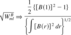
(Appendix A). This is the asymptotic distribution that arises also when the analogous Wald statistic is calculated from the AR0(1) model; again the ARμ(1) model would yield a different distribution or (24) (Dickey and Fuller, 1979).
A comparable LR statistic is

The asymptotic unit-root distribution of this statistic, after standardization, is

(Appendix A). It can be shown by standard unit-root asymptotic results that this is the distribution of the corresponding LR statistic, T(LRml0 − 1), under the AR0(1) model also (proof omitted). The T(LRml0 − 1) statistic essentially equals the usual F = t2 statistic, with obvious notation, for the null of a unit root. It gives intuition for the fact that the preceding asymptotic distribution of T(LRmlB − 1) is the square of that of

.
The agreement of the asymptotic unit-root distributions of the statistics extends to the case of a near unit root (Section 10). By simple arguments, the agreement holds also in the stable case (for the MLE and Wald statistics considered by the author).
4. ADJUSTED PROFILE LIKELIHOOD
In this section, ψ and φ are considered as a general parameter of interest and a vector of nuisance parameters, respectively. The APL of Cox and Reid (1993) is

Here

is the k × k observed information matrix for φ or −∂2l(ψ, φ)/∂φ∂φ′ (with (i,j)th element jφiφj) evaluated at

, the coefficient c is defined by

its MLE being

or c evaluated at the MLEs of ψ and φ, Iφφ is the Fisher information matrix with (i,j)th component iφiφj, and iφψ is the Fisher information vector with (i,1)th element iφiψ or iφψ = E [−∂2l(ψ, φ)/∂φ∂ψ] .
If ψ and φ are orthogonal or iφψ = 0 then the coefficient c, and its MLE

, collapse to zero and, helpfully, only the two first terms of the APL need to be calculated. This will turn out to be the case under the ARB(1) model. Oddly enough, the coefficient can equal zero even if the parameters are not orthogonal, as in the ARB(1) model with an unrestricted x0 in Appendix C. In the ARμ(1) model the parameters are nonorthogonal and the coefficient has to be calculated (Pere, 1997, 2000). Some intuition for the APL under orthogonality is given in the next section.
The value of ψ that maximizes (14) is the adjusted estimator (AE) of ψ or

. An adjusted Wald statistic for the null hypothesis ψ = 1 is defined as

(Pere, 1997, 2000). An analogous adjusted LR statistic is
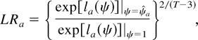
where the power is set for convenience only for the application to follow. The statistics and the corresponding asymptotic distributions, under the ARB(1) model with a unit root, are calculated in the next section.
5. ADJUSTED PROFILE LIKELIHOOD ANALYSIS AND UNIT-ROOT ASYMPTOTICS FOR THE ARB(1) MODEL
Under the ARB(1) model ψ is advantageously orthogonal with respect to γ and σ2 and the latter to each other:

The following equality was already touched on when (8) was contemplated:

The number 1 in (19) arises from the first observation, whereas the term (T − 1)(1 − ψ)2 ensues from the rest of the observations. Hence the first observation remains the most informative on γ as long as ψ ≠ 0. If ψ = 0 then all observations are equally informative.
The final information measure to note is an observed measure:

These calculations yield

and the APL:

The term −½ log[1 + (T − 1)(1 − ψ)2] pushes

to the right of

on the real axis if

, but it shrinks

downward if

. The term is nonpositive and penalizes large values of (1 − ψ)2 or small values of ψ when the parameter space is restricted to (−1,1]. Absorbingly, the term diminishes as ψ approaches 1 and vanishes at 1. A divergent maximum of the APL can be excluded because there is a bounded solution for the minimum of

by Section 3 and the potential divergence of the second term of (20) to minus infinity would be boosted if ψ diverged.
A way to interpret the Cox–Reid adjustment in general is that it penalizes values of ψ that provide relatively more information on the nuisance parameters. The phenomenon is quite explicit here: iγγ is minimized at ψ = 1, and other more informative values are penalized as a simple function of iγγ.
A kind of degrees-of-freedom correction emerges to the multiplier of

. By numerical experiments, this adjustment may increase or decrease the estimate compared to the case where T − 3 is replaced by the usual T (cf. (6)). An enlargement arises if

, whereas a subtraction results if

. Therefore the correction strengthens the adjustment due to the term −½ log[1 + (T − 1)(1 − ψ)2] .
It can be inferred from (20) that the MLE and AE share the same asymptotic distribution under a unit root: the terms

and [1 + (T − 1)(1 − ψ)2] are of the same magnitude for ψ ∈ (−1,1] (Op(T) or Op(1) when evaluated at ψ ∈ (−1,1) or ψ = 1, respectively). Logs are taken of both terms in (20), but the second term becomes negligible for large T because the first term is multiplied by −(T − 3)/2. Hence the first term determines both the MLE and AE for large T.
The adjusted likelihood equation

can be shown to be equivalent to a fifth-order polynomial in ψ, so numerical methods are needed to find

. The equation is guaranteed to possess a real root because the order of the polynomial is odd.
The second derivative of the APL is needed to construct the WaB statistic of (16):

The formula for

is supplied in Appendix A. Despite absence of an analytical formula, the numerical value of WaB is easily found by substituting

in (16) and (22).
The adjustment does not alter the asymptotic unit-root distribution of the (signed square root of the) Wald statistic:

The convergence to zero of the additive adjustment (T − 1)[1 − (T − 1) × (1 − ψ)2]/{T2[1 + (T − 1)(1 − ψ)2]2}, evaluated at

, is easily reasoned:

is Op(T−1) under ψ = 1, so the effect is Op(T) over T2. The other convergencies are explained in Appendix A.
The adjusted LR statistic is from (17)

The term

does not play a part in the asymptotic distribution of T(LRaB − 1) under a unit root:

converges in probability to zero, so

converges in probability to unity. It follows that T(LRaB − 1) shares the same asymptotic unit-root distribution with T(LRmlB − 1) or

6. STATISTICS AND UNIT-ROOT ASYMPTOTICS FOR THE ARμ(1) MODEL
Under the ARμ(1) model the MLE of ψ and the Wald statistic for the unit-root null hypothesis are

where

, and the formulation of the Wald statistic is akin to (12) (Pere, 2000). The estimator

is also the ordinary least-squares (OLS) estimator. The AE for ψ under the ARμ(1) model is essentially

where

is (1 − ψ)−1 − (1 − ψT)/[T(1 − ψ)2] evaluated at

. The formula for

applies for a large T, but in the simulations that follow the exact definition given in Pere (2000) is employed. The adjusted Wald statistic of (16) is

(Pere, 2000).
The conventional statistics tend to the following well-known unit-root distributions as T increases:

where

(e.g., Pere, 2000).
2There is a misprint in the B*(1) formula in Pere (2000, p. 339). The term B*(1) should be denoted by B*(r) and be as Bμ(r) in the current notation.

(Pere, 2000). The LR statistics are not inspected under the ARμ(1) model.3
Under the ARμ(1) model with (ψ,α) = (1,0), one might presume that an LR unit-root test for the joint hypothesis (ψ,α) = (1,0) renders a more powerful test than one focusing on ψ only. However, in the simulations of Dickey and Fuller (1981) the test did not yield a gain in power. An explanation is that

, with obvious notation, absorbs changes in the level of the time series due to an altered initial value, say, and is comparable to the in general inessential constant of an ordinary linear regression.
7. FRACTILES FOR THE UNIT-ROOT ARB(1) MODEL
The small-sample unit-root fractiles of the standardized coefficients (SCs),

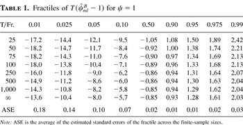
, are reported in Tables 1 and 4 (based on simulations reported in Appendix D). These fractiles (and those in Tables 6, 7, 8, and 9 for the Wald and LR statistics) apply irrespective of the nuisance parameters γ and σ2, or the initial value x0, now relaxed to take any finite value, by the invariance and similarity results in Appendix C.
Fractiles of for ψ = 1

The median of the distribution of

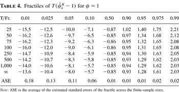
is negative and the left tail is the longer, which suggest a biased estimator for all sample sizes. For observations in excess of 50 the fractiles essentially monotonically tend toward zero, or the distribution becomes more compact.
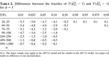
The fractiles are compared with the (unreported) corresponding distribution under the AR0(1) model in Table 2. Two sample sizes are printed on most lines of the table (say, 24–25). The larger is the last observed time period and the smaller is the number of observations available for estimation of the AR0(1) model (Section 2). (Parallel notation applies to Tables 3, 12, and 13.)
Differences between the fractiles of for ψ = 1

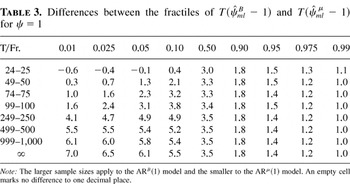
Engrossingly, when the sample size is small the left-tail fractiles under the ARB(1) model lie far to the left of the corresponding left-tail fractiles under the AR0(1) model. It increases the bias and spread of the MLE in comparison to the latter model. Moreover, the distribution under the former converges to the asymptotic fairly slowly. The ARB(1) model establishes invariance with respect to the initial value at the cost of inaccuracy in estimation in comparison with the AR0(1) model and does not yield small-sample distributions that are as dense as the asymptotic distribution suggests. The small-sample left-tail fractiles under the ARB(1) model fit better with (and lie in general to the right of) those for the ARμ(1) model (Table 3). In large samples these fractiles naturally differ.
Differences between the fractiles of for ψ = 1

The 0.05th fractiles of

are reported in Pantula et al. (1994) also. These fractiles are smaller than those in Table 1 for samples of 25 and 50 apparently because, by unreported simulations with the OPTMUM module of GAUSS 3.2.17 (1992), the simple algorithm employed in Pantula et al. (1994) yields left-tail fractiles that are too small.
Zivot (1994, p. 564), focusing on the unit-root case, reasons that

takes similar values to

or the MLE of ψ calculated from the AR0(1) model treating y1 as the initial value.
4Zivot's formula (37) for S2(ρ,x0) agrees with (7) here for

after substituting ψ for ρ. Zivot wrote that “S2(μ,x0) … is minimized near

, the OLS estimate of ρ in the simple AR(1) model without an intercept.” (Here S2(μ,x0) looks like a misprint for S2(ρ,x0) because the former was not defined in the paper nor does it have ρ as an argument.)

for ψ = 1. However, unreported simulation experiments reveal that the similarity holds only under a (near) unit root and a fairly large sample size (cf. Table 2). Otherwise the estimators can take very different values.
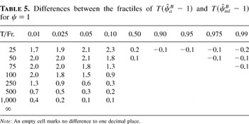
The adjustment cuts both tails of the distribution of the MLE but especially the left tail (Tables 4 and 5). Moreover, in essence all the fractiles of the AE—except the asymptotic fractiles copied from Table 1—lie closer both to zero and to the asymptotic fractiles than those of the MLE. The AE seems less biased and variable, or more accurate, and follows the common asymptotic distribution better than the MLE.
Fractiles of for ψ = 1

Differences between the fractiles of for ψ = 1

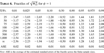
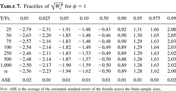
The fractiles of the Wald statistics

are in Tables 6 and 7. The location and shape of the distributions vary less with the sample size than those of the SCs. Yet the distribution of

is more concentrated in general and matches much better with the common asymptotic distribution in small samples. Both statistics take a real value for all draws. However, unreported simulation experiments uncover that

can take a complex value if T is extremely small, such as 5.
Fractiles of for ψ = 1

Fractiles of for ψ = 1

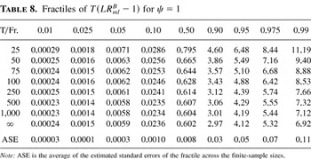
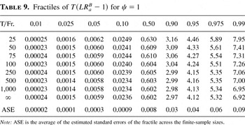
Tables 8 and 9 contain the fractiles for the LR statistics. The adjustment cuts the tails of the small-sample distributions so that LRaB follows the common asymptotic distribution far better than LRmlB.
Fractiles of T(LRmlB − 1) for ψ = 1

Fractiles of T(LRaB − 1) for ψ = 1

8. FRACTILES FOR THE UNIT-ROOT ARμ(1) MODEL
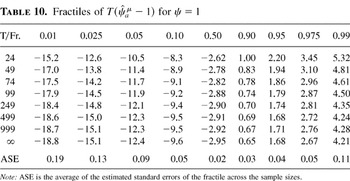
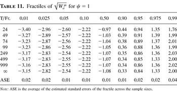
Fractiles of the finite-sample and the asymptotic unit-root distributions of

are reported in Tables 10 and 11. We found that

was real in all of the simulations. The fractiles are invariant with respect to the initial value (Pere, 2000). The constant α is fixed to zero, but the magnitude of σ2 is irrelevant for the fractiles (proof omitted). The distributions are discussed and the details of the simulations are in Pere (1997, 2000).
Fractiles of for ψ = 1

Fractiles of for ψ = 1

9. COMPARING ESTIMATION ACCURACY
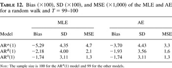
The bias, standard deviation (SD), and mean-square error (MSE) of the MLE and AE for a random walk under the different AR(1) models are shown in Table 12. The number of observations is 100 for estimation of the ARB(1) model and one less for the other models (Section 2). The AE and MLE are the same under the AR0(1) model (Pere, 1997).
Bias (×100), SD (×100), and MSE (×1,000) of the MLE and AE for a random walk and T = 99–100

The bias, SD, and MSE of the estimators decrease uniformly in absolute value from the top to the bottom row. The ARμ(1) model is by far the worst with respect to each of the quantities. The statistics for the ARB(1) model are clearly smaller yet are inferior to the statistics for the AR0(1) model. The adjustment improves estimation accuracy in terms of bias and MSE under the ARμ(1) and ARB(1) models and also in terms of SD under the latter. Under a unit root this holds even asymptotically under the former model (Pere, 2000). This is possible because the standard regularity conditions behind the usual optimality results for the MLE are not valid under nonstationarity.
Unreported simulation experiments indicate that if the sample size is exceptionally small, say, 10 or less, then the AE is an overwhelmingly better estimator than the MLE under the unit-root ARB(1) model. This is due to the dominance of the unit-root-favoring term of the APL, −½ log[1 + (T − 1)(1 − ψ)2] , when the sample is uninformative.
10. NEAR UNIT-ROOT ASYMPTOTICS UNDER THE ARB(1) MODEL
In the case of a near unit-root or ψ = exp(δ/T), δ < 0 (Phillips, 1987) corresponding asymptotic distributions apply:

In the preceding expressions i is an index for ml or a, and

is an Ornstein–Uhlenbeck process. The proofs for i = ml are in Appendix A. The adjusted statistics follow the same distributions as the unadjusted by similar logic as in the unit-root case (Section 5 and Appendix A). Phillips (1987) has discovered that the first two asymptotic distributions apply (and it can be shown that the third distribution also applies) for the corresponding statistics under the AR0(1) model with a near unit root. Thus the unit-root and near unit-root distributions of the respective statistics are identical under the ARB(1) and AR0(1) models. It follows that the respective unit-root tests are asymptotically equally powerful against near unit-root alternatives whether or not the adjustment is employed and regardless of which of the two models is used.
11. NEAR UNIT-ROOT ASYMPTOTICS UNDER THE ARμ(1) MODEL
The asymptotic distributions of

, under ψ = exp(δ/T) and α = 0, are known to be

where

(e.g., Stock, 1994, p. 2772). It is proved in Appendix B that the adjusted statistics follow different distributions under the same assumptions:

The power of the respective unit-root tests against near unit-root alternatives is likely to differ, even asymptotically, under the ARμ(1) model.
12. UNIT-ROOT TESTS AND POWER COMPARISONS FOR THE ARB(1) MODEL
The unit-root fractiles of

permit testing of ψ = 1 under the ARB(1) model for various sample sizes. Large values of the LR statistics and small values of the other statistics suggest rejection of the null.
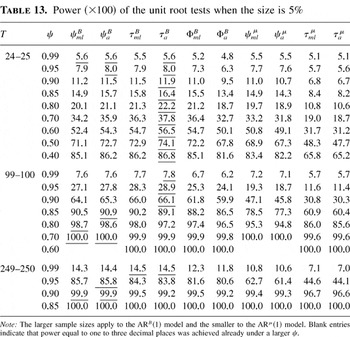
The tests based on the SCs will be denoted by ψmlB and ψaB with obvious notation. The corresponding Wald and LR tests will carry the labels τmlB, τaB, ΦmlB, and ΦaB. The simulated powers of the tests are in Table 13. The test size is 5%, and the ranges of ψ and T are 0.4–0.99 and 24–25 to 249–250. The larger sample sizes apply in this section.
Power (×100) of the unit root tests when the size is 5%

The ψaB test is as powerful as or slightly more powerful than the ψmlB test.5
The combination ψ = 0.8 and T = 99–100 is an exception.
The Wald tests are as powerful as or more powerful than the corresponding SC tests when there are 25 observations, contrary to the well-known ranking under the ARμ(1) model (next section).6
The ψmlB and τmlB tests are an exception at ψ = 0.99.
The LR tests are never the most powerful and compare unfavorably to the rest of the tests. The ΦmlB test can possess more power than a SC or Wald test under T = 25 only, and the weakest test is ΦaB. Some intuition is that the LR tests are two-sided, whereas the other tests are one-sided.
13. UNIT-ROOT TESTS AND POWER COMPARISONS FOR THE ARμ(1) MODEL
The tests associated with the

statistics will be referred to as ψmlμ, ψaμ, τmlμ, and τaμ. Their powers are in Table 13 also.
7The statistics

employ the MLE of σ instead of the degrees-of-freedom corrected estimator as in Dickey and Fuller (1979). The estimator of σ affects the scale of the null distributions, but power is unaffected. The simulation algorithm accepts the null of a unit root if it comes across a noncalculable

(for details, see Pere, 1997, 2000). Another alternative would be to exclude such instances, which would, if anything, increase the power estimates for the τaμ test.
The adjusted versions of the tests tend to be a bit weaker in contrast to the ARB(1) case. The differences in power are in general larger between the SC than between the Wald tests. As a by-product, Table 13 affirms the Monte Carlo results of Dickey, Bell, and Miller (1986, Table 2), Dickey and Fuller (1979, p. 430), and Schmidt and Phillips (1992): the ψmlμ test is often substantially more powerful than the τmlμ test.
14. POWER COMPARISON BETWEEN THE TWO AR(1) MODELS
Even though the ARB(1) and ARμ(1) models agree under the null, the time series, or the underlying processes against which the powers are evaluated, can differ despite a common AR coefficient. The time series match, up to the long-run mean, when x0 = y0 − α/(1 − ψ) = 0 (Section 2) or when both time series have started from the respective long-run mean. The power figures for the models can be compared under this assumption meaningfully.
Underlining indicates the most powerful test in Table 13. In case of a tie a number of tests are indicated except on the lines where all tests achieve power of unity.
The ψmlB test is in general more powerful than the ψmlμ test. The difference in power can be very large but is small for 24–25 observations. The latter outcome is intuitively due to the similarity of the small-sample distributions of the associated MLEs (Table 3). The ψaB test is the most powerful of the SC tests for all sample sizes (but see note 5). The τmlB and τaB tests tend to be far more powerful than the corresponding τmlμ and τaμ tests, so that at its best the τaB test can possess more than twice the power of the τmlμ or τaμ test. This is largely because the powers of the Wald tests do not fall short of the powers of the SC tests under the ARB(1) model as happens under the ARμ(1) model.
Tests gain power much faster under the ARB(1) than the ARμ(1) model as the number of observations increases. For example, the powers (×100) for the ψmlμ test under ψ = 0.95 at sample sizes of 24 and 249 are 7.7 and 62.7. The corresponding figures for the ψmlB test are 7.9 and 85.7. The relative gain is even larger for the Wald tests: the analogous figures for them are 5.7 and 44.6 vs. 7.9 and 84.3.
The ARB(1) model always yields more powerful tests. The benefit in power (×100) from using the ARB(1) model is 5.7% units at its best for 24–25 observations (τaB vs. ψmlμ at ψ = 0.6) and swells to 19% units for 99–100 observations (τaB vs. ψmlμ at ψ = 0.90) and to 23.1% units for 249–250 observations (ψaB vs. ψmlμ at ψ = 0.95).
The adjustment does not necessarily increase power. The adjustment decreases power under the ARμ(1) model and power of LR tests under the ARB(1) model. Nevertheless, in general the most powerful test employs the adjustment (but see note 5).
The τaB test is, among the inspected tests and values of ψ, the most powerful at sample size of 25 and the most powerful for ψ close to unity at sample size of 99–100. Among the same sets, no test is always the most powerful for sample sizes of 99–100 and 249–250.
15. DISCUSSION
The ARB(1) model is an innovative way to present nuisance parameters orthogonally to the AR coefficient. Estimation of the constant does not affect the asymptotic distribution of the standardized MLE even in the unit-root case. The model can yield more accurate estimates and powerful tests of a unit root than the conventional model. A disadvantage is that the time series is restrictively assumed to initialize from the long-run mean.
The Cox–Reid adjustment is lucid and intuitive. Under the unit-root ARB(1) model a simultaneous cutback in bias, variance, and MSE over the MLE can be achieved with the adjustment in small samples.
The adjusted statistics follow the asymptotic unit-root distributions better than their unadjusted counterparts when the model is ARB(1). The same outcome has been found previously when the model is ARμ(1) and the process is a random walk with drift or stable and 0 ≤ ψ < 1 (Pere, 2000) or when the process is a stationary AR(1) with the initial value obeying the stationary distribution (Cruddas, Reid, and Cox, 1989). Thus the Cox–Reid adjustment is able to bring the small-sample distribution closer to the asymptotic distribution whether the process is stable or nonstationary or whether the asymptotic distribution is standard (such as normal) or a unit-root distribution.
A point of statistical interest is that if the initial value of the unobserved AR(1) underlying the ARB(1) process is allowed to differ from zero then the parameters become nonorthogonal whereas the adjustment remains unmodified.
The derived tests are invariant with respect to the initial value and similar. The τaB test is the most powerful for the smallest inspected sample size, but for larger samples no single test dominates when the model is ARB(1). Under the same model, an LR test is never the most powerful, and the performance of the LR tests is deficient. For the ARμ(1) model the ψmlμ test is the most powerful.
Powers under the two models can be meaningfully compared under the assumptions that the time series follow an ARB(1) process, that the ARμ(1) model is estimated conditional on y1, and that the time series have started from their respective long-run means. The ARB(1) model yields more powerful tests so that the difference in power increases with the sample size (within the inspected range) and can become very large.
The adjustment does not inevitably increase power, as exemplified by the LR tests for the ARB(1) model and the tests for the ARμ(1) model. Nevertheless, the τaB test appears the most powerful for very small sample sizes, and in general the most powerful tests utilize the adjustment. The benefit from the adjustment is clearer for small sample sizes, because the adjustment fades asymptotically.
Many empiricists use the τmlμ test even though the ψmlμ test is more powerful. Now with very small samples, at least, there is reason to employ a Wald test but one derived from the ARB(1) model. The finding matches with the result of Pantula et al. (1994, p. 452) that in general, apart from the ψmlμ and τmlμ tests, Wald-type tests tend to be more powerful if the time series starts from the long-run mean. No single test possesses the highest power for all sample size and parameter combinations.
The results on power would not change essentially (by unreported simulations) if the power comparisons were based on an equal number of observations or had the AR0(1) or ARμ(1) model generated the data to which the ARB(1) model would have been fitted. The ARB(1) model would still furnish the more powerful tests, and the most powerful tests would still tend to employ the adjustment.
Robinson (1994) and Saikkonen and Luukkonen (1997) also utilize a model in which the interpretation of deterministic terms is not dependent on the stationarity status of the underlying time series. Robinson's unit-root tests enjoy asymptotic optimality properties against fractionally integrated alternatives, whereas the cointegration tests of the latter authors possess superior power performance over conventional tests. Because the asymptotic distribution theory in these papers is not affected by the deterministic terms, similarly to this paper, this contemporary way of introducing deterministicity seems beneficial in more general settings, too.
APPENDIX A: NEAR UNIT-ROOT ASYMPTOTICS FOR THE ARB(1) MODEL
Calculations in this Appendix are valid under

Straightforward calculations would show that the relevant sums entailing innovations and observations under the near unit-root ARB(1) process yield the standard asymptotic convergencies employed subsequently. The unit-root results follow by setting δ = 0.
Proving That

and Equals y1 Asymptotically under a Near Unit Root. The PL for γ is

where

and

is defined in (10). Some algebra, the relation yt = γ(1 − ψ) + ψyt−1 + εt for t ≥ 2, and well-known orders of magnitude of the sums imply that

By simple arguments it can be confirmed from the preceding expression that

—the solution to the minimization problem

—cannot diverge. The minimization problem is thus infγ[(y1 − γ)2 − γOp(T−1/2)], which yields

for large T.
Approximations for

under a Near Unit Root. Substitution of yt = γ + ψ(yt−1 − γ) + εt for t ≥ 2 to the second line of (11) and the approximations T(ψ − 1) = δ + O(T−1) = O(1) from (A.1) yield

One could find the asymptotic distribution directly from the preceding expression. Instead, an approximation is developed—to be used later—from which the distribution can be reasoned. From the preceding expression

where the last equality is a consequence of (A.1). It follows that

under ψ = exp(δ/T). The asymptotic near unit-root distribution of

is in (25). The distribution can be inferred from (A.4) or (A.5), because statistics of which

is composed share the same asymptotic distributions whether the generating model is ARB(1) or AR0(1).
By Op(1)ness of

, (A.1), and (A.5):

under ψ = exp(δ/T).
Consistency of

Evaluated at the MLE or AE under a Near Unit Root. Consistency of

, evaluated at

of ψ under a near unit root, is easily proved by substituting (A.6) into (7). Consistency of

can be proved similarly.
Asymptotic Distribution of the Wald Statistic under a Near Unit Root. An important ingredient of the Wald statistic is ∂2lp(ψ)/∂ψ2:

(cf. (9)), where


The Wald statistic

, the ingredients appropriately standardized, is

The derivatives of

—of which ∂2lp(ψ)/∂ψ2 is composed—become multiplied by powers of T. By definition,

, evaluated at

, equals zero. The asymptotic distribution of the standardized second derivative, evaluated at

, is nondegenerate:

where

. By these results and the consistency of

, the asymptotic distribution of

is

where

is substituted on the second line and convergencies (25) and (A.8) and consistency of

are employed.
Construction and Near Unit-Root Asymptotics of T(LRmlB − 1). From (7) and (13):

where

The asymptotic distribution of T(LRmlB − 1) under the null of a near unit root will be derived. For this purpose, a few intermediate results on orders of magnitude are needed. First,

is Op(T1/2) by superconsistency of

. The numerator of

is hence

An asymptotic expression for the denominator of

is likewise found to be

by (A.5). Thus,

is

These results and (A.5) yield the following expression for the denominator of LRmlB:

Finally, the asymptotic distribution can be derived:

(accuracy in the denominator can be relaxed)

The convergence follows from (25), consistency of

under the ARB(1) model by (A.5) and (A.6), and Phillips (1987, p. 539).
APPENDIX B: NEAR UNIT-ROOT ASYMPTOTICS FOR THE ARμ(1) MODEL
The asymptotic distributions for the adjusted statistics under the ARμ(1) model with ψ = exp(δ/T) and α = 0 are derived. It is assumed that the statistics are calculated conditional on y0.
Near Unit-Root Asymptotics for the MLE of ψ. The well-known asymptotic near unit-root distribution of

is

Recalling (A.1), it follows that

or that

The final standard result to point out is that the denominator of

.
Near Unit-Root Asymptotics for the AE of ψ. The AE of (23) equals

The preceding approximation derives from the first-order Taylor expansion around unity of

. Here x > −1 is assumed and the remainder term r1 = −1/8(1 + ax)−3/2x2 where a ∈ (0,1) by Taylor's theorem. The orders of magnitude of r1,T and rT are due to

being

being Op(T−1) under a near unit root, as is shown subsequently.
To find the asymptotic near unit-root distribution of

, one needs the corresponding distributions for

. The derivation in Pere (2000, p. 348) applies here by substituting DFδμ in place of DFμ there. This gives

The next task is to derive the asymptotic near unit-root distribution for

. The asymptotic distribution and probability limit of the terms in the multiplication have been derived already in (B.1) and (B.2), respectively. The last term can be written as

The asymptotics of the denominator is the same as that of

, so, after multiplication by T−2, it converges weakly to

. An approximation for the numerator, yT(yT − 2y−1) + Op(T1/2), can be found similarly to the case under a unit root (Pere, 2000, p. 356). The numerator multiplied by T−1 is

Thus

It follows from (B.1), (B.2), and the preceding result that

Combining (B.1), (B.3), (B.4), and (B.5) yields

Near Unit-Root Asymptotics for the Adjusted Wald Statistic. A formulation of

is

(Pere, 2000, (5), (18), and (23)). The form for the ratio derived on p. 358 of Pere (2000) extends straightforwardly by the previous results to the near unit-root case. Hence

Here rT* is Op(T−2). The convergence follows from (B.5) and (B.6).
APPENDIX C: INVARIANCE AND SIMILARITY RESULTS FOR THE ARB(1) MODEL
If the process is a random walk then a meaningful estimator and test statistic of ψ should not depend on the value from which the process was initialized (x0). Such an invariance property of the MLE and AE under a unit root is proved subsequently for the ARB(1) model. Invariance of the associated Wald and LR statistics, under a unit root, follows straightforwardly. Next, invariance of the statistics with respect to multiplication of the data is verified. Similarity of the associated unit-root tests is a direct consequence of these results. The PL is again a useful tool for proving the claims. The scrutinized statistics are based on x0 = 0 even though x0 ≠ 0 is allowed for. Related results for the ARμ(1) statistics have been proved in Pere (2000).
Addition of a constant a to the observations converts

(see (8)). The residual variance of (7),

remains unchanged. Thus

is tied to its original value regardless of an added constant. The adjustment term of (21) also remains unmodified, as does

.
If ψ = 1, then x0 ≠ 0 has an analogous effect on yt as adding a constant to yt after the generation of it. It follows that

is undisturbed by x0 ≠ 0 if ψ = 1, and one can allow for x0 ≠ 0 when testing for a unit root via

ψmlB.
Invariance of

with respect to x0 under ψ = 1 is not obvious because some of the influence measures, on which the adjustments rest, are disturbed by x0. The formula

permits a nonzero x0 and is the basis for the following calculations (cf. (7) for x0 = 0). A sole information measure of relevance needs revision:

The parameters are nonorthogonal unless x0 = 0, so the term

should be included in APL (14). However, the term is superfluous because c equals zero:

because neither of the information measures in the parentheses is a function of γ ((18) and (19)). The conclusion is that

is not affected by x0 under ψ = 1, so it can be used as a basis for a unit-root test allowing for x0 ≠ 0.
The proposed unit-root tests are invariant with respect to multiplication of the data by a constant: the tests are derivatives of

. Multiplication of the yt's by a constant h transfers the estimators to

by (7). The factor h2 does not affect maximization of the PL or APL, and hence the SC statistics, and cancels when the LR statistics are constructed. In the calculation of the Wald statistics log h2 differentiates out.
Similarity of the tests follows straightforwardly. A change in γ corresponds to addition of a constant to the observations and is irrelevant as explained before. Multiplying the innovations by h or altering σ2 to hσ2 has the same effect as multiplication of the yts by h if γ = x0 = 0 (cf. (3)), which is inconsequential as explained previously. The same alteration is inconsequential even if γ ≠ 0 or x0 ≠ 0 because any constant including γ or x0 can be deducted from the data first, without affecting the analysis as reasoned earlier, and the previous argument can be applied next. The tests are hence similar whether x0 = 0 or x0 ≠ 0.
APPENDIX D: ON THE SIMULATIONS
The GAUSS 3.2.17 (1992) simulation programs in essence (excluding the code for the LR tests) are given in Pere (1997). The advancement here is that the simulations entail 300,000 draws composed of 10 subsamples with different seeds and the power results for the ARB(1) model involve 100,000 draws. Such splitting is recommended by Abadir (1995) for strongly autocorrelated processes to lessen dependence of the results on a seed. The set of seeds is common for each value of ψ when simulating power. The GAUSS code for performing the simulations is available from the author upon request.
In the estimation of the asymptotic fractiles Brownian motions are approximated with random walks (zt) of length 10,000. For example, ∫[B(r)]2 dr is approximated by

.
The statistics for the ARB(1) model are found numerically with the default optimization algorithm in the OPTMUM 3.1.4 module of GAUSS using initial value of unity for ψ. Under a unit root, the magnitude of γ does not theoretically alter the MLE. With OPTMUM, however, a large γ may decelerate convergence apparently indefinitely (Pere, 1997), so it was fixed at zero for the present results. Relatedly, the program may not reproduce exactly the same results if two different values of σ2 are experimented with. The explanation is that if OPTMUM enters a random search in an iteration, different sequences of time series arise despite a common set of seeds for two Monte Carlo experiments.
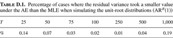
Appropriate convergence of the algorithm was confirmed by recording the proportion of cases in which the residual variance is not smaller at the MLE, according to the algorithm. The proportion was very small when simulating the fractiles (Table D.1). In the few inspected incidents, numerical inaccuracy was the explanation because the variances departed in the eighth decimal place, say.
Percentage of cases where the residual variance took a smaller value under the AE than the MLE when simulating the unit-root distributions (ARB(1))

Table 2 is constructed so that for each draw of a time series the MLEs under the ARB(1) and AR0(1) model are computed. For the latter model the MLE is conditional on y1, which is random instead of fixed as in (5), but it should not be consequential. The fractiles for the MLE under the ARμ(1) model, needed for Table 3, are calculated conditional on y1, too, but the randomness does not affect the fractiles (Appendix C). Table 12 is constructed analogously to Tables 2 and 3. The fractiles (for each sample size) and the results on power (for each value of ψ), respectively, are based on the same seeds but not necessarily the same time series as explained earlier.
References
REFERENCES
Abadir, K.M.
(1995)
A new test for nonstationarity against the stable alternative.
Econometric Theory
11,
81–104.Google Scholar
Ahn, S.K.
(1993)
Some tests for unit roots in autoregressive-integrated-moving
average models with deterministic trends.
Biometrika
80,
855–868.Google Scholar
Andrews, D.W.K.
(1993)
Exactly median-unbiased estimation of first order
autoregressive/unit root models.
Econometrica
61,
139–165.Google Scholar
Bhargava, A.
(1986)
On the theory of testing for unit roots in observed time series.
Review of Economic Studies
52,
369–384.Google Scholar
Cox, D.R. &
N. Reid
(1987)
Parameter orthogonality and approximate conditional inference.
Journal of the Royal Statistical Society, Series B
49,
1–39.Google Scholar
Cox, D.R. &
N. Reid
(1993)
A note on the calculation of adjusted profile likelihood.
Journal of the Royal Statistical Society, Series B
55,
467–471.Google Scholar
Cruddas, A.M.,
N. Reid, &
D.R. Cox
(1989)
A time series illustration of approximate conditional likelihood.
Biometrika
76,
231–237.Google Scholar
Dickey, D.A.
(1976)
Estimation and Hypothesis Testing in Nonstationary Time Series.
Ph.D. thesis.
Iowa State University.
Dickey, D.A.,
W.R. Bell, &
R.B. Miller
(1986)
Unit roots in time series models: Tests and implications.
American Statistician
40,
12–26.Google Scholar
Dickey, D.A. &
W.A. Fuller
(1979)
Distribution of the estimators for autoregressive time series with
a unit root.
Journal of the American Statistical Association
74,
427–431.Google Scholar
Dickey, D.A. &
W.A. Fuller
(1981)
The likelihood ratio statistics for autoregressive time series with
a unit root.
Econometrics
49,
1057–1072.Google Scholar
Elliot, G.,
T.J. Rothenberg, &
J.H. Stock
(1996)
Efficient tests for an autoregressive unit root.
Econometrica
4,
813–836.Google Scholar
The GAUSS System Version 3.0
(1992) Washington, D.C.: Aptech Systems.
Hansen, H. &
A. Rahbek
(2002)
Approximate conditional unit root inference.
Journal of Time Series Analysis
23,
1–28.Google Scholar
Lee, J. &
P. Schmidt
(1994)
Unit root tests based on instrumental variables estimation.
International Economic Review
35,
449–462.Google Scholar
Neyman, J. &
E.L. Scott
(1948)
Consistent estimates based on partially consistent observations.
Econometrica
16,
1–32.Google Scholar
Pantula, S.G.,
G. Gonzalez-Farias, &
W.A. Fuller
(1994)
A comparison of unit-root test criteria.
Journal of Business and Economic Statistics
12,
449–459.Google Scholar
Pere, P.
(1997)
Adjusted Profile Likelihood Applied to Estimation and Testing of
Unit Roots.
D.Phil. thesis,
University of Oxford.
Pere, P.
(2000)
Adjusted estimates and Wald statistics for the AR(1) model with
constant.
Journal of Econometrics
98,
335–363.Google Scholar
Phillips, P.C.B.
(1987)
Towards a unified asymptotic theory for autoregression.
Biometrika
74,
535–547.Google Scholar
Phillips, P.C.B. &
P. Perron
(1988)
Testing for a unit root in time series regression.
Biometrika
75,
335–346.Google Scholar
Robinson, P.M.
(1994)
Efficient tests of nonstationary hypotheses.
Journal of the American Statistical Association
89,
1420–1437.Google Scholar
Saikkonen, P. &
R. Luukkonen
(1997)
Testing cointegration in infinite order vector autoregressive
processes.
Journal of Econometrics
81,
93–126.Google Scholar
Schmidt, P. &
J. Lee
(1991)
A modification of the Schmidt–Phillips unit root test.
Economics Letters
36,
285–289.Google Scholar
Schmidt, P. &
P.C.B. Phillips
(1992)
LM tests for a unit root in the presence of deterministic time
trends.
Oxford Bulletin of Economics and Statistics
54,
257–287.Google Scholar
Seber, G.A.F. &
C.J. Wild
(1989)
Nonlinear Regression.
New York:
Wiley.
Stock, J.H.
(1994)
Unit Roots, Structural Breaks and Trends. In
R.F. Engle &
D.L. McFadden (eds.),
Handbook of Econometrics,
vol. 4.
Amsterdam:
North-Holland.
West, K.D.
(1988)
Asymptotic normality, when regressors have a unit root.
Econometrica
56,
1397–1417.Google Scholar
Zivot, E.
(1994)
A Bayesian analysis of the unit root hypothesis within an
unobserved components model.
Econometric Theory
10,
552–578.Google Scholar
Fractiles of for ψ = 1
Differences between the fractiles of for ψ = 1
Differences between the fractiles of for ψ = 1
Fractiles of for ψ = 1
Differences between the fractiles of for ψ = 1
Fractiles of for ψ = 1
Fractiles of for ψ = 1
Fractiles of T(LRmlB − 1) for ψ = 1
Fractiles of T(LRaB − 1) for ψ = 1
Fractiles of for ψ = 1
Fractiles of for ψ = 1
Bias (×100), SD (×100), and MSE (×1,000) of the MLE and AE for a random walk and T = 99–100
Power (×100) of the unit root tests when the size is 5%
Percentage of cases where the residual variance took a smaller value under the AE than the MLE when simulating the unit-root distributions (ARB(1))
 You have
Access
- 2
- Cited by