1. Introduction
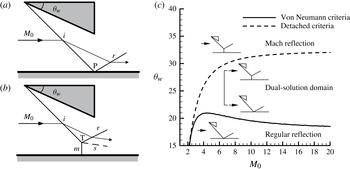
As described by Ben-Dor (Reference Ben-Dor1999), there are two possible shock reflection configurations in steady supersonic flow, one is named regular reflection (RR) and the other is named Mach reflection (MR). They are illustrated in figure 1(a,b), respectively. Aiming at the transition between RR and MR, von Neumann (Reference von Neumann1943) proposed two extreme criteria, which would later be renamed the detached criteria and the von Neumann criteria. Then, a new concept of shock reflection hysteresis was introduced by Hornung, Oertel & Sandeman (Reference Hornung, Oertel and Sandeman1979). They indicated that there exist a region where both RR and MR are possible between the detached criteria and the von Neumann criteria in steady supersonic flows. The region is characterized as the dual-solution domain, which is pointed out in figure 1(c). Thereafter, the hysteresis phenomena was confirmed experimentally by Chpoun et al. (Reference Chpoun, Passerel, Li and Ben-Dor1995) and numerically by Vuillon, Zeitoun & Ben-Dor (Reference Vuillon, Zeitoun and Ben-Dor1995). Also, some researchers conducted investigations to better understand the three-dimensional effects (see Skews Reference Skews2000), real gas effects (see Gimelshein, Markelov & Ivanov Reference Gimelshein, Markelov and Ivanov1998) and dynamic effects (see Naidoo & Skews Reference Naidoo and Skews2011) on the transition between RR and MR in steady flows.
It should be noted that in the above-mentioned studies of shock reflection hysteresis, the reflecting plane is always replaced by the surface of symmetry, in order to eliminate the viscous effects. While, Henderson (Reference Henderson1976) analytically investigated the shock reflection configurations at a rigid wall, which is helpful to know the complex wave system that is generated when an incident shock interacts with the boundary layer. However, this conclusion is based on the hypothesis that the interacting phenomenon is treated as the refraction of a shock by a boundary layer which is replaced by an inviscid shear layer. Afterward, little work has been conducted on the shock reflection considering the boundary layer along the reflecting plane. For these reasons, further studies are needed to make a better understanding of the shock reflection phenomenon, after the boundary layer effects are taken into account.
Schematic illustration of shock reflection configurations and the domains of possible shock reflection pattern in the
 $M_{0}{-}{\it\theta}_{w}$
plane. (a) Regular reflection (RR) and (b) Mach reflection (MR). Here
 $M_{0}$
is the free-stream Mach number,
 ${\it\theta}_{w}$
is the wedge angle,
 $i$
is the incident shock wave,
 $r$
is the reflected shock wave,
 $m$
is the Mach stem,
 $s$
is the slip line, P is the reflected point and T is the triple point.

Hence, it is important to take shock wave–boundary layer interaction into consideration when investigating the viscous effects of shock reflection hysteresis in this study. Combining the free-interaction theory with the shock reflection hysteresis theory, a detailed analysis that was conducted to clarify the viscous flow fields of shock reflection pattern is presented in § 2. Moreover, the experimental results of two shock reflection patterns, and the numerical results of a hysteresis process that is induced by changing the free-stream Mach number, are performed to verify the analytical results in § 3, respectively. Conclusions are summarized in § 4.
2. Theoretical model
It is generally known that a complex wave configuration may occur when a shock is reflected by the flat plate. Owing to viscous effects, the incident shock imposes a strong adverse pressure gradient on the boundary layer, which may drive it to thicken or to separate. In view of the above problems, Chapman, Kuhen & Larson (Reference Chapman, Kuhen and Larson1957) suggested the free-interaction theory to describe the shock wave–boundary layer interactions. They gave the following expression for the pressure rise during the interaction:
 $$\begin{eqnarray}\frac{p-p_{0}}{q_{0}}=\overline{\,f}(x)\frac{\sqrt{2C_{f0}}}{(M_{0}^{2}-1)^{1/4}}\end{eqnarray}$$
where
 $$\begin{eqnarray}q_{0}=\frac{{\it\gamma}}{2}p_{0}M_{0}^{2}.\end{eqnarray}$$
Here,
 ${\it\gamma},p_{0},q_{0}$
and
 $M_{0}$
denote the specific heat ratio, the free-stream static pressure, the free-stream dynamic pressure and the oncoming flow Mach number, respectively. It should be noted that the free-stream Mach number
 $M_{0}$
is set beyond the value of 2.202 for diatomic perfect gases, in order to study the viscous effects of the shock reflection hysteresis phenomenon, because the von Neumann criteria are invalid when
 $M_{0}<2.202$
(see Mölder Reference Mölder1979).
Also,
 $\overline{f}(x)$
is employed to denote a dimensionless correlation function along the streamwise coordinate. Babinsky & Harvey (Reference Babinsky and Harvey2011, p. 53) indicated that the value of
 $\overline{f}(x)$
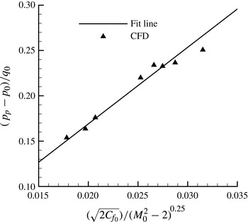
corresponding to the interactional region in laminar flow is 1.5, and that it is 6 in turbulent flow. However, the mentioned values do not apply to all situations. It may be affected by the Reynolds number. Figure 2 gives numerical results of the shock wave–boundary layer interaction when the Reynolds number per unit based on the free-stream conditions range from
 $7\times 10^{6}$
to
 $1.1\times 10^{7}$
. The straight line is a least-squares fit to the simulative points. Consequently, the dimensionless correlation function
 $\overline{f}(x)$
in turbulent flow can be achieved by measuring the slope of the fit line, and its value is equal to 8.5.
Numerical results of the shock wave–boundary layer interaction and the least-squares fitting line when the Reynolds number per unit based on the free-stream conditions range from
 $7\times 10^{6}$
to
 $1.1\times 10^{7}$
.

In addition,
 $C_{f0}$
is the skin-friction coefficient of the interaction origin
 $x_{0}$
. Further, the value of
 $C_{f0}$
can be obtained through the equation (see Sivells & Payne Reference Sivells and Payne1959):
 $$\begin{eqnarray}C_{f0}=0.088\frac{T_{0}}{T_{c}}\cdot \frac{lg(k\cdot \mathit{Re}_{x_{0}})-2.3686}{(lg(k\cdot \mathit{Re}_{x_{0}}-1.5)-1.5)^{3}}\end{eqnarray}$$
where
 $T_{0}$
is the free-stream temperature and
 $\mathit{Re}_{x0}$
is the local Reynolds numbers at the interaction origin
 $x_{0}$
. For the determination of the compressible skin-friction coefficient, a variable
 $T_{c}$
named reference temperature is induced,
 $$\begin{eqnarray}T_{c}=0.22(T_{aw}-T_{0})+0.5(T_{0}+T_{w}).\end{eqnarray}$$
In (2.4),
 $T_{w}$
is the wall temperature and
 $T_{aw}$
is the adiabatic wall temperature. The midterm function
 $k$
which is mentioned above is expressed in
 $$\begin{eqnarray}k=\frac{{\it\mu}_{0}T_{0}}{{\it\mu}_{c}T_{c}},\end{eqnarray}$$
and
 ${\it\mu}_{0}$
and
 ${\it\mu}_{c}$
are the viscosity coefficient at
 $T_{0}$
and
 $T_{c}$
, respectively. They could be obtained from the conventional relation for the temperature variation of
 ${\it\mu}$
based on Sutherland’s law,
 $$\begin{eqnarray}\frac{{\it\mu}}{{\it\mu}_{a}}=\left(\frac{T}{T_{a}}\right)^{3/2}\cdot \frac{T_{a}+T_{s}}{T+T_{s}}.\end{eqnarray}$$
For air at standard conditions, when
 $T_{a}=273.16\ \text{K}$
,
 ${\it\mu}_{a}=1.7161\times 10^{-5}\ \text{Pa}\ \text{s}$
and Sutherland constant
 $T_{s}=124\ \text{K}$
.
In addition, the equation for the local Reynolds numbers,
 $\mathit{Re}_{x0}$
is given by
 $$\begin{eqnarray}\mathit{Re}_{x_{0}}=\frac{P_{0}M_{0}x_{0}}{{\it\mu}_{0}}\cdot \sqrt{\frac{{\it\gamma}}{RT_{0}}},\end{eqnarray}$$
and the equations for the adiabatic wall temperature,
 $T_{aw}$
, are
 $$\begin{eqnarray}\displaystyle T_{aw}\approx T_{0}+\frac{{\it\gamma}-1}{2}\mathit{Pr}^{1/3}T_{0}M_{0}^{2},\quad (\text{turbulent boundary layers}). & & \displaystyle\end{eqnarray}$$
 $$\begin{eqnarray}\displaystyle T_{aw}\approx T_{0}+\frac{{\it\gamma}-1}{2}\mathit{Pr}^{1/2}T_{0}M_{0}^{2},\quad (\text{laminar boundary layers}). & & \displaystyle\end{eqnarray}$$
 $\mathit{Pr}$
), that is a property of the gas is introduced. For air at standard conditions,
 $\mathit{Pr}=0.71$
and the gas constant
 $R=287\ \text{J}\ \text{kg}^{-1}\ \text{mol}^{-1}$
.
Based on the hypothesis that
 $T_{w}$
and
 $x_{0}$
keep invariable during the interaction, the plateau pressure of the interactional region
 $p_{p}$
can be calculated from the follow expression, according to the (2.1)–(2.8):
 $$\begin{eqnarray}\frac{p_{p}}{p_{0}}=g(M_{0},P_{0},T_{0}).\end{eqnarray}$$
From (2.9), it is apparent to know that the value of
 $p_{p}$
is decided by the flow conditions. Then the question whether the separated region appears or not is discussed, combined with the shock reflection configurations. In figure 1(a), the static pressure
 $p_{inciscid1}$
behind the reflected shock can be obtained from the theory of oblique shock waves. On the one hand, if
 $p_{inviscid1}>p_{p}$
, the boundary layer is induced to thicken. Also, it is essential to make sure whether the flow field which consists of a MR configuration can exist without separation. In general, the pressure rise across a Mach stem is approximately equal to the pressure jump through a normal shock at the same free-stream Mach number. Thus, the pressure rise across the Mach stem can be obtained by
 $$\begin{eqnarray}\frac{p_{inviscid2}}{p_{0}}=\frac{2{\it\gamma}}{{\it\gamma}+1}M_{0}^{2}-\frac{{\it\gamma}-1}{{\it\gamma}+1}.\end{eqnarray}$$
Using (2.1) and (2.10), we obtain
 $$\begin{eqnarray}\displaystyle & \displaystyle y_{0}=\frac{p_{inviscid2}}{p_{0}}-\frac{p_{p}}{p_{0}}=\frac{2{\it\gamma}}{{\it\gamma}+1}M_{0}^{2}-\frac{\sqrt{2}{\it\gamma}\overline{f}(x)\cdot M_{0}^{2}}{2(M_{0}^{2}-1)^{1/4}}\cdot \sqrt{C_{f0}}-\frac{{\it\gamma}-1}{{\it\gamma}+1}-1, & \displaystyle\end{eqnarray}$$
 $$\begin{eqnarray}\displaystyle & \displaystyle y_{0}<g_{1}(M_{0})=\frac{2{\it\gamma}}{{\it\gamma}+1}M_{0}^{2}-\frac{\sqrt{2}{\it\gamma}\overline{f}(x)\cdot M_{0}^{2}}{2(M_{0}^{2}-1)^{1/4}}-\frac{{\it\gamma}-1}{{\it\gamma}+1}-1. & \displaystyle\end{eqnarray}$$
 $M_{0}>2.202$
,
 $y_{0}$
is always beyond zero. It also means that the MR configuration without separation is not physical. In another words, the shock reflection hysteresis does not exist when the boundary layer is induced to thicken.
On the other hand, if
 $p_{inviscid1}<p_{p}$
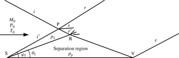
, the boundary layer separates. Figure 3 gives the schematic illustration of the shock reflection configuration with separation. A incident shock
 $i$
interacts with a separation shock
 $i^{\prime }$
which is generated by the separation region SRV, at reflection point P. The separation region is also known as the isobaric dead-air region, that means the static pressure in it is always equal to
 $p_{p}$
. Then, SR is the isobaric boundary, a relationship between the static pressure
 $p_{1}$
behind the separation shock
 $i^{\prime }$
and
 $p_{p}$
is given by
 $$\begin{eqnarray}p_{1}=p_{p}.\end{eqnarray}$$
Schematic illustration of shock wave–boundary layer interactions with separation: S, separation point; P, reflection point; V, reattachment point; R, peak of the separation region;
 $e$
, reattachment shock;
 $i$
, incident shock;
 $i^{\prime }$
, separation shock;
 $r$
and
 $r^{\prime }$
, reflected shock;
 $s$
, slipline.

Further, the angle of separation shock
 ${\it\varphi}_{1}$
and the compression angle of the separation region
 ${\it\theta}_{1}$
can be achieved through the following equations:
 $$\begin{eqnarray}\displaystyle & \displaystyle \frac{p_{1}}{p_{0}}=1+\frac{{\it\gamma}}{{\it\gamma}+1}(M_{0}^{2}\sin ^{2}{\it\varphi}_{1}-1) & \displaystyle\end{eqnarray}$$
 $$\begin{eqnarray}\displaystyle & \displaystyle \tan {\it\theta}_{1}=2\cot {\it\varphi}_{1}\frac{M_{0}^{2}\sin ^{2}{\it\varphi}_{1}-1}{M_{0}^{2}({\it\gamma}+\cos (2{\it\varphi}_{1}))+2}. & \displaystyle\end{eqnarray}$$
From the above equations, it is simple to find that the value of
 ${\it\theta}_{1}$
is independent of the incident shock strength. Also, the value of
 $C_{f0}$
changes slightly, even though
 $x_{0}$
changes substantially. Based on these conclusions, we assume that the separation region is replaced by a wedge, which has an angle of
 ${\it\theta}_{1}$
. Moreover, the viscous effects of the wall have little influence on the reflection point P, so we can use pressure-deflection shock polars to analyse the shock reflection configuration. If
 $M_{0},P_{0}$
and
 $T_{0}$
are set as 4, 5527.9 Pa and 216.69 K, respectively (turbulent boundary layers),
 ${\it\theta}_{1}$
can be obtained from the above equations, and the value is
 $15.45^{\circ }$
. Then, the hypothetical wedge angle is fixed, while the wedge angle
 ${\it\theta}_{2}$
varies from small to large. According to the theory of asymmetric shock reflection (see Li, Chpoun & Ben-Dor Reference Li, Chpoun and Ben-Dor1999; Ivanov et al.
Reference Ivanov, Ben-Dor, Elperin, Kudryavtsev and Khptyanovsky2002), the type of shock reflection during this process is discussed theoretically.
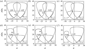
Figure 4 gives six shock polars to illustrate the possible solutions of reflection configuration. When
 ${\it\theta}_{2}=15.45^{\circ }$
, we can obtain the shock polar combination shown in figure 4(a) which indicates that an overall RR wave configuration and an overall MR wave configuration are theoretically possible. However, the overall MR that consists of two inverse MRs (InMRs) is not physical. When
 ${\it\theta}_{2}$
is increased to
 $23^{\circ }$
, an overall RR and an overall MR that consist of a direct MR (DiMR) and an
 $I_{n}MR$
are predicted from the shock polar shown in figure 4(b). It is noteworthy that this type of MR with a diverging slipstream tube which is formed by two slips lines is non-existent actually, because it conflicts with the subsonic flow behind the Mach stem.
Shock polars when the wedge angle
 ${\it\theta}_{2}$
increases at
 $M_{0}=4$
.

In figure 4(c), when
 ${\it\theta}_{2}$
is equal to
 ${\it\theta}^{N}$
, three polars meet at point S. If
 ${\it\theta}_{2}>{\it\theta}^{N}$
, the diverging slipstream tube is replaced by a converging slipstream tube, although the possible overall MR still consists of an
 $I_{n}MR$
and a
 $D_{i}MR$
. The solution of shock polar combination shown in figure 4(d) means that there exists two flow structures under the uniform flow condition theoretically, one is overall RR, the other is overall MR with a converging slipstream tube, when the value of
 ${\it\theta}_{2}$
rises to
 $32^{\circ }$
.
In figure 4(e),
 ${\it\theta}^{D}$
indicates the angle of maximum deflection, while
 ${\it\theta}^{E}$
means where the polars are tangent. Li et al. (Reference Li, Chpoun and Ben-Dor1999) suggests that an overall RR which consists of a strong RR and a weak RR appears when
 ${\it\theta}^{D}<{\it\theta}_{2}<{\it\theta}^{E}$
. Thus,
 ${\it\theta}^{D}$
and
 ${\it\theta}^{N}$
are two extreme situations between which both an overall RR and an overall MR are possible in theory. Upon further increase in
 ${\it\theta}_{2}$
to
 $35^{\circ }$
, the shock polar combination shown in figure 4(e) illuminates the overall MR with a converging slipstream tube is the unique solution.
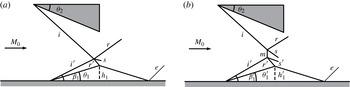
Based on the foregoing discussion, figure 5 gives a schematic illustration of two possible shock reflection configurations considering the boundary-layer effects. Similarly to the inviscid structure shown in figure 1(a), the wave pattern in figure 5(a) which is named overall RR does not have a Mach stem. It consists of an incident shock (
 $i$
), a separation shock (
 $i^{\prime }$
), two reflected shock (
 $r$
and
 $r^{\prime }$
), a separated region, a slip line (
 $s$
) and a reattachment shock (
 $e$
). In the overall MR wave configuration (figure 5
b), in addition to the above structures, a Mach stem (
 $m$
) appears, accompanied by a converging slipstream tube.
Shock reflection configuration considering the boundary-layer effects: (a) an overall RR and (b) an overall MR.

In short,
 ${\it\theta}^{N}$
is similar to the von Nenmann angle in the reflection of symmetric shock waves, and
 ${\it\theta}^{D}$
is similar to the detached angle. Thus, a dual-solution domain of shock reflection configuration can be obtained. It means that for the uniform flow conditions, we may obtain two flow fields when the wedge angle is fixed. If
 ${\it\theta}^{N}<{\it\theta}_{2}<{\it\theta}^{D}$
, the reflection types mentioned in figure 5 are both theoretically possible. In another words, a shock reflection hysteresis induced by changing the wedge angle
 ${\it\theta}_{2}$
or altering the free-stream Mach number can be expected, in spite of viscous effects.
3. Validation and discussion
3.1. Experimental study
The experiments are carried out in a continuous supersonic wind tunnel which is well described by He et al. (Reference He, Yi, Tian and Chen2011). Owing to the limit of experimental facility, the flow parameters are reset. Here,
 $M_{0},P_{0}$
and
 $T_{0}$
are 3, 2750 Pa and 107 K, respectively. Then, the Reynolds number per unit based on the free-stream conditions can be calculated, and its value is
 $7.4\times 10^{6}$
. Thus, the dimensionless function
 $\overline{f}(x)=8.5$
. At the same time, the interaction origin
 $x_{0}$
should be adjusted downwards, because of the geometric parameters of the model. The value is reduced to 10 % of unit length. Consequently, the separation region is replaced by a hypothetical wedge, and the angle
 ${\it\theta}_{1}=16.62^{\circ }$
.
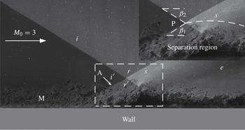
A high-spatiotemporal resolution image of shock reflection configurations considering the viscous effects use the NPLS technique corresponding to an overall RR in figure 5(a).

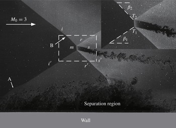
A high-spatiotemporal resolution image of shock reflection configurations considering the viscous effects use the NPLS technique corresponding to an overall MR in figure 5(b).

In these experiments, two shock reflection configurations which are mentioned above can be obtained, when the shock-generating wedge angle changes. However, the analytical hysteresis phenomenon has not been observed in the experiments. It may be caused by the upstream boundary-layer acoustic perturbations. Previous studies have indicated that the level of upstream disturbances is critically important for reproducing the shock reflection hysteresis (see Ivanov et al. Reference Ivanov, Kudryavtsev, Nikiforov, Pavlov and Shiplyuk2003b ). Further, except for one experiment conducted in the low-noise wind tunnel, experiments on the transition between RR and MR generally showed well that the transition angles is inside the dual solution domain, rather than at the theoretical limit (see Ivanov et al. Reference Ivanov, Kudryavtsev, Nikiforov, Khotyanovsky and Pavlov2003a ).
Figures 6 and 7 give two high-spatiotemporal resolution images of shock reflection configurations considering the viscous effects using the nanotracer planar laser scattering (NPLS) technique which is based on Rayleigh scattering and use the nanoparticles as tracer particles (see Zhao, Tian & Yi Reference Zhao, Tian and Yi2009). The photographs which are obtained by the above method can reflect fine structures of the complex interaction, rather than the flow field that is through temporal and spatial integration. In these pictures, vortex structures in the separation region which constitute a trigonal configuration can be identified clearly.
Figure 6 shows the reflection pattern of a shock wave at a flat wall in the presence of a turbulent boundary layer corresponding to an overall RR in figure 5(a) when the shock-generating wedge angle is 14.8°. Similarly, another reflection pattern shown in figure 5(b) is displayed in figure 7. In figure 6, the structures such as incident shock (
 $i$
), separation shock (
 $i^{\prime }$
), reflected shocks (
 $r$
and
 $r^{\prime }$
), and slip line (
 $s$
) are well presented. Moreover, symbol M is employed to denote the turbulent boundary layer. Due to the boundary-layer effects, the separation shock (
 $i^{\prime }$
) in region A converges to a smooth curve. Also, the flow field in figure 7 has the same phenomenon. Hence, the angle between the straight line near the reflection point P (or the triple point
 $T_{1}$
) and a horizontal line is acted as the separation shock angle. In figure 7, as a result of the interaction of the expansion waves that emanate from the trailing edge of the wedge, and three-dimensional effects, the incident shock (
 $i$
) in region B is curved. Similarly to the separation shock, the incident shock angle should be adjusted to the angle between the straight line near the triple point
 $T_{2}$
and a horizontal line, rather than the wedge angle.
After measurement, the separation shock angles (
 ${\it\beta}_{1}$
) in figures 6 and 7 are 33.41 and 33.34°, respectively. From them,
 ${\it\theta}_{1}$
corresponding to
 ${\it\beta}_{1}$
can be calculated by the (2.15), and the values are 16.11 and 16.05°, respectively. Further analysis indicates that the experimental value are approximately 3 % smaller than the analytical results, which is mainly caused by the disparity in interaction origin. Also,
 ${\it\beta}_{2}$
and
 ${\it\theta}_{2}$
can be achieved in the same way. Here,
 ${\it\beta}_{2}=32.03^{\circ }$
,
 ${\it\theta}_{2}=14.8^{\circ }$
in the overall RR configuration, while
 ${\it\beta}_{2}=46.45^{\circ }$
,
 ${\it\theta}_{2}=26.61^{\circ }$
in the overall MR configuration.
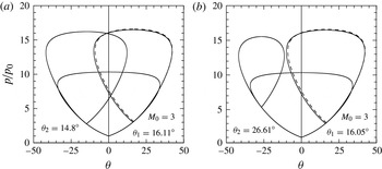
Two shock polar combinations at
 $M_{0}=3$
: (a)
 ${\it\theta}_{1}=16.11^{\circ }$
,
 ${\it\theta}_{2}=14.8^{\circ }$
corresponding to the shock reflection configuration in figure 6; (b)
 ${\it\theta}_{1}=16.05^{\circ }$
,
 ${\it\theta}_{2}=26.61^{\circ }$
corresponding to the shock reflection configuration in figure 7. The dashed polar is corresponding to the analytical angle, and the value is
 $16.62^{\circ }$
.

Figure 8 presents two shock polar combinations corresponding to the experimental conditions at
 $M_{0}=3$
. And the dashed pressure-deflection shock polar corresponds to the theoretical angle. Despite the slight discrepancy in
 ${\it\theta}_{1}$
between the experimental and the analytical value, the shock polar solution shown in figure 8(a) represents a typical overall RR configuration shown in figure 5(a). Also, an overall MR configuration can be expected with the aid of the shock polar shown in figure 8(b).
Hence, the experimental results indicate that the analysis can be well applied to predicting the viscous interaction configurations, although the hysteresis phenomenon is not confirmed by experiments. At the same time, the two theoretical shock reflection configurations which are mentioned in figure 5 are confirmed.
3.2. Numerical study
Similarly to the hysteresis phenomenon in the steady reflection of asymmetric shock waves, a shock reflection hysteresis considering viscous effects can be excepted. Based on the solution in figure 4(d) which is inside the dual-solution domain, the wedge angle
 ${\it\theta}_{2}$
and the oncoming Mach number are set as 32° and 4, respectively, for verifying the hysteresis phenomenon.
3.2.1. Numerical methods
In this paper, the two-dimensional compressible Navier–Stokes equations are expressed in the cell-centred finite volume formulation, and are solved by using Roes second-order scheme. Then, ideal gas model with the specific heat ratio
 ${\it\gamma}=1.4$
is employed. Also, the sketch of the computational domain was given in figure 9. Further, to avoid the grids affect the accuracy of flow field, the computational grid should have high orthogonality and smoothness. The value of
 $y^{+}$
is set smaller than 1 for all of the flow fields, and
 $y^{+}$
of the wall is approximately equal to 0.1. The minimum value of
 $y$
corresponding to
 $y^{+}$
is marked by
 $y_{min}$
, and
 $y_{min}/H_{1}=6.25\times 10^{-6}$
. The coarse grid for the hysteresis calculations is
 $350\times 100$
. To ensure the resolution of results, the mesh is refined based on a pressure gradient criterion as well as along the surface of the wall, and the total number of cells is 200 000.
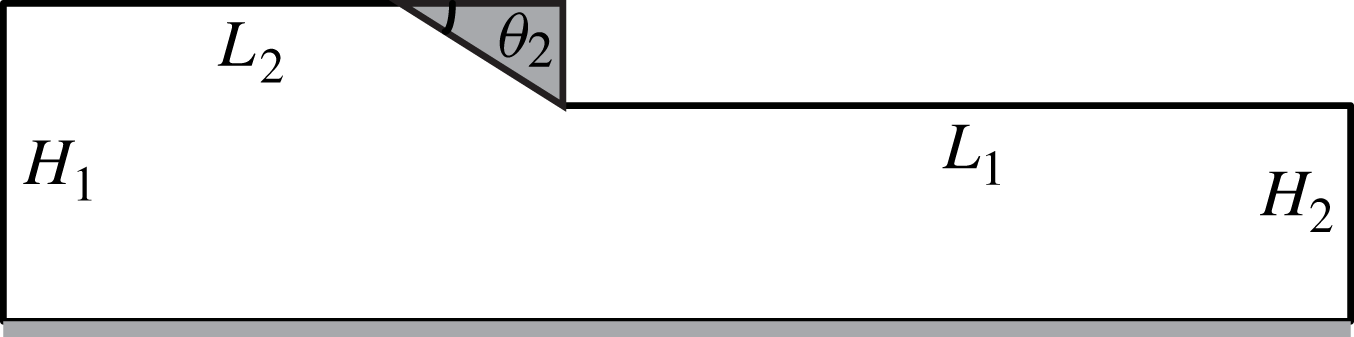
A sketch of the computational domain.
 $H_{1}=0.4\ \text{m}$
,
 $H_{2}=0.275\ \text{m}$
,
 ${\it\theta}_{2}=32^{\circ }$
,
 $L_{1}=1\ \text{m}$
and
 $L_{2}=0.5\ \text{m}$
.

As we all know, numerical simulation of flow separation in steady supersonic flow is a challenging task, so it is critical to select a turbulence model for a better result. Also, no one can deny the fact that the standard
 ${\it\kappa}{-}{\it\varepsilon}$
model is inefficient in predicting an accurate separation region. While the viscous-affected region of the boundary layer can be properly resolved, by using the Spalart–Allmaras (SA) model, in accordance with the previous statement and in agreement with previous work (see Spalart & Allmaras Reference Spalart and Allmaras1992).
3.2.2. Hysteresis phenomenon
Based on the analytical result in figure 4(d), we keep the wedge angle
 ${\it\theta}_{2}$
constant and change the free-stream Mach number
 $M_{0}$
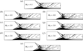
to investigate the hysteresis phenomenon. The Mach number contours of the flow-Mach-number-variation-induced hysteresis process in the transition between overall RR and overall MR as achieved numerically is shown in figure 10. When the computational region is installed in a uniform supersonic flow with initial Mach number
 $M_{0}=4.1$
, the flow field in figure 10(a) consists of an overall RR is the unique solution. When the flow Mach number is reduced from 4.1 to 3.8, the overall RR wave configuration is retained. As
 $M_{0}$
is reduced continually, an overall MR wave pattern appears at
 $M_{0}=3.7$
in figure 10(e). From figure 10(d,e), it is easy to find that the transition from overall RR to overall MR takes place when the free-stream Mach number changes from 3.8 to 3.7. In another words, we can conclude that the overall RR
 $\longrightarrow$
overall MR transition happens at
 $M_{0}=3.75\pm 0.05$
.
The shock reflection hysteresis process during variation of the flow Mach number at
 ${\it\theta}_{2}=32^{\circ }$
.

Figure 10(e) gives the unique flow structure which consists of an overall MR at
 $M_{0}=3.7$
. Then, the flow Mach number is increased back to 4.1. From figure 10(e–h), the overall MR wave configuration remains during the variety of Mach numbers, despite the height of the Mach stem shortens gradually. However, when the oncoming Mach number is increased to 4.1, the Mach stem disappears, and the overall MR wave pattern is replaced by the overall RR wave configuration. Furthermore, the overall RR
 $\longleftarrow$
overall MR transition occurs at
 $M_{0}=4.05\pm 0.05$
. Thus, a shock reflection hysteresis process which is composed by the transition between the overall RR and the overall MR considering the viscous effects is obtained.
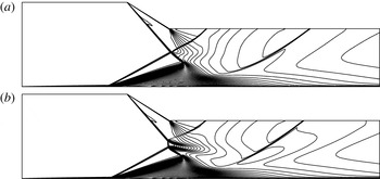
The detailed flow fields of the shock reflection at
 $M_{0}=4$
are given in figure 11. From the pictures, numerical results illuminate that there exist two different shock reflection patterns for the same physical model under the uniform flow conditions, thereby verifying the analytical conclusions. In order to gain a better understanding of the hysteresis phenomenon, it is essential to quantitate the geometrical parameters of the above flow fields. In this paper, the shock angles are measured through the oblique shock wave equations, and the angle of the separation region is calculated by (2.15). In addition, as the skin friction coefficient at the separation point is equal to zero,
 $x_{\mathit{separation\;point}}$
can be estimated. However, it is not sufficient to calculate the height of Mach stem (
 $h_{Mach\,stem}$
) in an overall MR configuration, unless the horizontal coordinate of the Mach stem (
 $x_{Mach\,stem}$
) is known.
The Mach number counters of the shock reflection pattern when
 $M_{0}=4$
: (a) an overall RR; (b) an overall MR.

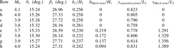
Table 1 gives the values during the shock reflection hysteresis process at
 ${\it\theta}_{2}=32^{\circ }$
. From it, we can find that the angle of separation region ranges from 15.24 to 15.33°, due to the fluctuation of
 $M_{0}$
and
 $x_{0}$
. Also, this table illuminates that the height of separation region in an overall RR wave configuration is much larger than that in an overall MR wave pattern, when the flow Mach number is uniform. Then, comparing the results in row b with those in row h, we can make a conclusion that the separation point in the overall MR is in the latter horizontal position, i.e.
 $x_{\mathit{separation\;point}_{oMR}}>x_{\mathit{separation\;point}_{oRR}}$
. The same conclusion can be obtained from row c and row g, row d and row f.
Values during the shock reflection hysteresis process at
 ${\it\theta}_{2}=32^{\circ }$
.

During the transition from an overall RR to an overall MR, the value of
 $x_{\mathit{separation\;point}}$
is reduced gradually, with the oncoming Mach number decreases. After the overall MR wave configuration appears, the Mach stem occurs. At the same time, the height of separation region decreases suddenly, and
 $x_{\mathit{separation\;point}}$
increases sharply.
Considering the transition from overall MR to overall RR, the Mach stem moves downstream, when the free-stream Mach number increases step by step. Also, the height of Mach stem is reduced gradually, during the transition. From the varieties of
 $h_{1}/H_{1}$
and
 $x_{\mathit{separation\;point}}/L_{2}$
, the conclusion that the separation region grows up and moves downstream during the process can be achieved. When the flow Mach number increases to 4.1, the Mach stem disappears. Also, the position of the separation point, the height of the separation region changes obviously. Thus, an overall RR wave configuration occurs again.
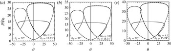
Afterwards, the reasons for the hysteresis process are discussed, combined with the shock polars shown in figure 12. In figures, the dashed polars are corresponding to the analytical angles, and the values are 15.72, 15.45 and 15.45°, respectively. Although the discrepancy between the numerical values and the analytical values still exist, which is influenced by the interaction origin
 $x_{0}$
. It has little effect on predicting the shock reflection configuration. When
 $M_{0}=3.7$
, it can be deduced from figure 12(a) that the overall MR is the unique flow field. It also is confirmed by the calculation results. Based on foregoing conclusions, the flow field at
 $M_{0}=3.8$
has two solutions, one is an overall MR the other is an overall RR.
Three shock polar combinations at different free-stream Mach numbers: (a)
 $M_{0}=3.7$
, (b)
 $M_{0}=3.8$
and (c)
 $M_{0}=4.1$
. The dashed polars are corresponding to the analytical angles.

However, the overall RR is the unique flow field when
 $M_{0}=4.1$
, despite the flow conditions being in the dual-solution domain. Two possible reasons can be listed as follows. First, the resolution of grids is beyond the height of Mach stem. Second the unsteady character of the separation region makes the overall MR configuration unstable when the height of the Mach stem is small. For the moment, few studies have been conducted for estimating the height of the Mach stem in asymmetric shock reflection. Hence, further studies are needed to clarify the hysteresis process.
In a word, similarly to the hysteresis phenomenon of symmetric shock waves in steady flow, a shock reflection hysteresis induced by altering the free-stream Mach number is confirmed numerically. Despite there being some differences between the analytical results and the numerical results, it is meaningful to simplify the problem for studying the shock reflection hysteresis when the viscous effects are taken into consideration.
4. Conclusions
The shock reflection hysteresis in steady supersonic flow has been investigated analytically, experimentally and numerically. In addition, it should be noted that the boundary layer that developed over the reflecting surface is taken into consideration in this paper.
Also, a simple wave interaction model has been introduced to represent the complex viscous wave configurations. Afterwards, the above method of evaluate the physical process is confirmed by the experimental and numerical results.
Based on the free-interaction theory and the shock reflection hysteresis theory, the analytical investigation is carried out to clarify the viscous flow field of shock reflection pattern. In order to describe the shock reflection configurations in detail, a hypothesis that the interaction origin
 $x_{0}$
remains invariable during the interaction is given. In addition, the separation region can be replaced by a hypothetical wedge. Then, by using shock polars, the existence of the hysteresis phenomenon that there are two possible flow structures under the same flow conditions is exemplified theoretically. Afterwards, the shock reflection structures in the dual-solution domain (
 ${\it\theta}^{N}<{\it\theta}_{2}<{\it\theta}^{D}$
) are discussed.
Then, a series of experiments are conducted for investigating the viscous effects of shock reflection hysteresis. Owing to the acoustic perturbations, the hysteresis phenomenon is not observed successfully. However, the experimental images indicate that the analysis can be well applied to predicting the viscous interaction configurations. At the same time, the two possible shock reflection configurations which are mentioned in figure 5 are confirmed.
Finally, based on the analytical results, proper parameters have been chosen for confirming the shock reflection hysteresis. When the flow Mach number is reduced to 3.7, the transition from overall RR to overall MR occurs. However, the overall MR does not disappear until the oncoming Mach number increases to 4.1. Thus, a shock reflection hysteresis induced by keeping the wedge angle constant and altering the free-stream Mach number is confirmed numerically. Also, we pay attention to the values of the shock reflection configuration during the shock reflection hysteresis process, to gain a better understanding of the viscous effects. Further, the reasons for the shock reflection hysteresis are discussed, using the shock polar combinations.
Acknowledgements
We would like to gratefully acknowledge the help of Dr H. Lin who provided much of the experimental data. This work was supported by the National Natural Science Foundation of China NSFC grant 11372347. This support is gratefully acknowledged.