

1 Introduction
Employees of the United States federal government have access to a defined contribution pension plan known as the Thrift Savings Plan (TSP). As of November 2005, this plan held $171 billion in assets on behalf of 3,545,000 participants. Participants can allocate and transfer funds among several investment options. Participants can also take loans from their balances. The loan amount is withdrawn from the investment experience of the funds, and the amount is replaced with interest paid by the participant.
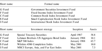
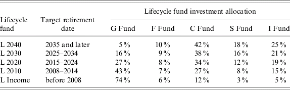
The TSP currently has five underlying investment options provided for in Title 5 of the US Code (5 USC §8438 (a)). Participants can allocate funds directly to one or more of these funds. These funds are shown in Table 1. Investors who want an age-appropriate asset allocation chosen for them can direct their investments to a ‘lifecycle’ fund. The lifecycle funds, introduced in August 2005, allocate investments among the five investment options given in Table 1. A description of these five lifecycle funds is given in Table 2.
Thrift Savings Plan investment funds

Note: Assets are as of December 2004 and in billions of dollars.
Source: Thrift Savings Plan Fund Information Sheets (2005).
Thrift Savings Plan lifecycle funds
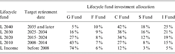
Notes: The lifecycle funds were introduced in August 2005 and allocate their assets to the five underlying funds. Each fund is designed for a different retirement cohort. Shown are target retirement dates and initial asset allocation for each lifecycle fund.
Source: Thrift Savings Plan Highlights, July 2005.
Of the five underlying funds, four are privately managed (currently by Barclays Global Investors). This includes the three equity index funds and the bond index funds. These four funds are very similar to funds available throughout the private sector.
The fifth fund, however, is not representative of investment opportunities available on the open market. This fund is called the Government Securities Investment Fund, or ‘G Fund’. The G Fund earns interest without any risk to principal and can be redeemed at par on short notice. In this sense, it resembles money market instruments such as Treasury bills. However, legislation sets the interest rate equal to the weighted average market yield (on the last day of the previous month) on Treasury securities with at least four years to maturity or call. In other words, the G Fund is a short-duration security with the yield of a long-duration security. Since the yield curve is generally upward sloping, this means the G Fund represents a riskless asset with an above-market rate of return.
The language setting the G Fund interest rateFootnote 1 substantially duplicates the language setting the rate on similar securities issued to the Social Security trust funds.Footnote 2 Each provision allows the maturity to be chosen in the interest of the respective fund. The TSP has consistently chosen very short maturities for the G Fund, and advertises this fact in the information sheet (2005) made available to participants.
In this paper, we examine the effect the G Fund has on participants' portfolios. We find that the G Fund has effects on participants' portfolios that do not simply represent portfolio reshuffling. This assessment allows us to make some qualitative welfare analysis of the Fund's impact.
The Thrift Savings Plan has been proposed both by the President's Commission on Social Security (2001) and by the Bush Administration itself (White House, 2005b) as a means to implement Social Security reform. Policymakers may be deciding whether to include the G Fund in such a system. We therefore briefly explore the role of the fund in Social Security reform.
2 The G Fund: a special stable value fund
Private sector stable value funds invest in intermediate term fixed income securities. The exact nature of these funds varies, but each promise their investors liquidity at par value plus accrued interest. Investors can undertake transactions at book value even when this differs from market value. This leads to a potential for arbitrage against the fund. For example, after an increase in interest rates, investors would have an incentive to move funds out of the stable value fund and into other fixed income funds. Any arbitrage trading will hurt the performance of the fund by redeeming assets at above their market value or selling new shares below their net asset value.
One method for alleviating this arbitrage pressure is to mitigate the fluctuations in market value of the assets held by the fund. For this reason, the duration of such funds is often kept low. For example, funds might use the net cash flow each month to purchase assets with a five year maturity. This would likely keep average maturity below three years.
Another method to alleviate arbitrage pressure is implicit or explicit restrictions on trading. These stable value funds are generally found in defined contribution pension plans, where such restrictions are possible to enforce. An example of an implicit restriction on trading would be the absence of other fixed income funds in the plan. Since stable value funds are protected from interest rate risk, arbitrage possibilities are especially strong using money market funds and inflation-indexed bond funds (which are protected from inflation risk but not real interest rate risk). An example of an explicit restriction would be an ‘equity wash’ rule that requires any transfers out of the stable value fund to stay in an equity fund for several months.
To the extent that these restrictions keep arbitrage trading low, the stable value fund can still provide superior returns to a money market fund if the yield curve is upward sloping. A ‘wrap’ insurance contract is purchased to guarantee that redemptions at par will be possible despite arbitrage losses. Investors are exposed to the credit risk of the company providing the wrap.
Unlike private sector stable value funds, the G Fund does not need to concern itself with such arbitrage losses. Since the G Fund effectively combines a money market fund with a stable value fund, there is no potential for arbitrage between these two asset classes. No restrictions are placed on G Fund transfers. The government has implicitly provided a default-free unlimited wrap contract at no cost. The yield on the G Fund, as mentioned above, is simply the average market yield on all marketable Treasuries with more than four years to maturity or call. As of December 2005, there was $1.375 trillion principal amount of such debt outstanding, with a weighted average time to maturity of 11.08 years. As a result, the G Fund return is based on assets further out the yield curve than a private sector stable value fund could safely hold. Further, investors do not suffer from any loss of the wrap fee or yield from arbitrage trading.
3 The popularity of the G Fund
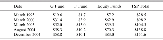
Treasury bills provide a measure of the return to a riskless security. Thrift Savings Plan data (2005) show that from 1988 through 2004, the G Fund returned 1.9% annually more than marketable three-month Treasury bills. The availability of the G Fund therefore represents a unique opportunity available to federal employees. Table 3 shows that federal employees take advantage of this opportunity by holding substantial G Fund balances. TSP participants seeking interest income have a choice between the G Fund and a standard bond index fund (the Fixed Income Index Investment Fund, or ‘F Fund’), which currently tracks the Lehman Brothers Aggregate bond index. The G Fund consistently attracts more than 80% of the assets allocated to the two fixed income accounts.
Thrift Savings Plan allocations
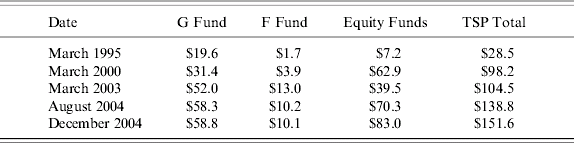
Note: Balances as of month end, in billions of dollars, and are taken from various issues of Thrift Savings Plan Highlights.
The large G Fund allocation reflects a relatively large allocation to riskless assets. Table 3 shows that TSP participants allocated $59 billion of their total TSP assets of $152 billion to the G Fund as of year-end 2004. Using the average yield advantage of 1.9%, this represents a subsidy of just over $1 billion to G Fund investors. To collect this $1 billion, TSP participants have constructed portfolios with a high share of the riskless asset.
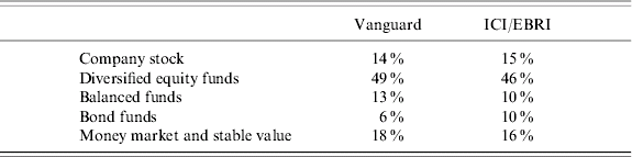
In contrast, private sector employees have constructed riskier portfolios. Table 4 shows data about the portfolio allocation of retirement funds. Portfolio weights are shown as of 2004 for Vanguard's defined contribution plans as well as of 401(k) plans conducted by the Investment Company Institute (ICI) and the Employee Benefit Research Institute (EBRI).
Pension fund allocations
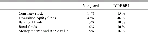
Notes: The middle column shows asset allocation in Vanguard defined contribution pension funds as of year-end 2004.
Source: Vanguard (2005: 21). The right column shows year-end 2004 asset allocation in the ICI/EBRI study of Holden and VanDerhei (Reference Holden and VanDerhei2005). In this study, assets in ‘minor investment options’ are not shown, resulting in the numbers adding to less than 100%.
In order to compare the private sector data in Table 4 with the TSP data, the private sector balanced fund holdings must be decomposed into equity, fixed income, and money market/stable value investments. These balanced fund portfolio weights have been estimated using a weighted average of Vanguard's balanced funds.Footnote 3 This has resulted in estimated balanced fund weights of 60% equity, 34% fixed income, and 6% money market. The 60% figure is also the weight Vanguard (2005) uses to estimate the equity exposure in balanced funds, although they do not decompose the 40% into fixed income and money markets. The Vanguard weights were also used to allocate the ICI/EBRI balanced funds. In addition, the ICI/EBRI allocations were scaled up to compensate for the reported 3% allocation to ‘minor investment options’.
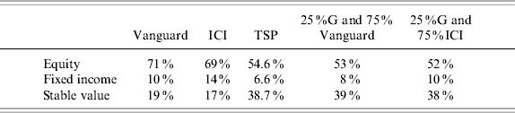
The resulting comparison for the TSP, Vanguard, and ICI/EBRI data is shown in Table 5. To estimate the change in behavior caused by the rate advantage of the G Fund, we can estimate the change in behavior required to make each private sector survey similar to the TSP allocation. An allocation of 24% to stable value funds plus 76% allocated to the observed Vanguard pattern would replicate the 39% stable value holdings of the TSP. Similarly, an allocation of 26% to stable value investments plus 74% to the observed ICI/EBRI allocation would replicate the 39% TSP value. The magnitude of the G Fund effect can therefore be estimated as having caused the allocation of about one-quarter of funds to the G Fund that would otherwise be allocated in the same way that other pension investors choose. The asset allocations resulting from allocating 25% to the G Fund and 75% to the portfolio weights in each of the alternative benchmarks are shown in Table 5.
TSP and private sector allocations
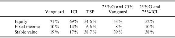
Notes: The Vanguard and ICI columns show the allocations in Table 4 reduced to the three major asset classes, while the TSP shows the same calculations for the TSP data in Table 3. The final two columns show the effect of allocating one-quarter of assets to the G Fund and three-quarters to the allocations shown by Vanguard and ICI/EBRI, respectively.
4 Portfolio distortion or portfolio reshuffling?
Thrift Savings Plan participants take advantage of the legislated G Fund yield subsidy by increasing their G Fund allocations above what benchmark data lead us to expect. In the previous section, it was shown that Thrift Savings Plan allocations resemble a two-step process. First, approximately one-quarter of the funds are allocated to the G Fund, and, second, the remaining three-quarters are allocated similarly to private sector benchmarks.
If investors are counteracting large G Fund holdings by holding a more risky portfolio outside of the TSP, then the overall effect of the G Fund subsidy is simply a change in asset location – that is, in which assets are held inside and outside the retirement account. The overall portfolio would be unchanged from what it would be without a G Fund. In this case, the presence of the 1.9% subsidy on the $57 billion in G Fund balances results simply in a transfer of approximately $1 billion from the federal government to its employees. This change in asset locationFootnote 4 could be described as portfolio reshuffling. Portfolio reshuffling is summarized in Table 6. Note that unless transaction costs are convex in the amount transacted, portfolio reshuffling is likely to lead to large transfers as the subsidy changes from positive to negative, or from negative to positive.
Portfolio reshuffling strategies

Note: In a pure portfolio reshuffling strategy, the G Fund subsidy does not affect overall portfolio risk, but simply the account in which risky and safe assets are held.
Portfolio reshuffling is impossible without a sufficient quantity of assets external to the TSP. There is evidence that many investors do not have these external assets. Bergstresser and Poterba (Reference Bergstresser and Poterba2004) findFootnote 5 that 45% of those with a tax-deferred account do not have any investments in taxable investments. Further, those with both taxable and tax-deferred accounts may have low balances in their taxable accounts. For example, Bergstresser and Poterba (Reference Bergstresser and Poterba2004: Table 4) find that of those with both taxable investments and tax-deferred investments, 25% have over six times the balance in their tax-deferred accounts as they do in taxable investments. Bergstresser and Poterba's results are based on the 2001 Survey of Consumer Finances, and do not distinguish between different types of tax-deferred accounts. It is possible that some TSP participants reshuffle between the TSP and other tax-deferred accounts,Footnote 6 such as individual retirement accounts or defined contribution accounts from previous employers. However, for a substantial fraction of TSP participants, full portfolio reshuffling is likely to be impossible.
If the shift of assets is not counteracted outside the TSP, then the G Fund is actually changing the asset allocation of the investor's portfolio. This effect can be called portfolio distortion. This portfolio distortion can be a rational response to the subsidy of the G Fund. To see this, consider an investor with assets only inside the TSP who has a mean-variance expected utility function

where μP and σP2 are the expected return and variance from the overall portfolio. For simplicity, consider the allocation between the G Fund and one risky asset. The G Fund has no risk but returns the risk free rate μ0 plus a subsidy S, while the risky asset has expected return μR and variance σR2. The expected return of this portfolio is

where w G the portfolio weight assigned to the G Fund. The variance of the portfolio is

Inserting these into equation (1) gives

The first order condition is then

which gives the optimal portfolio allocation to the G Fund as
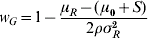
Note that a higher level of the subsidy S increases the portfolio weight w G assigned to the G Fund. This portfolio distortion results in a deadweight loss similar to that arising from any distortionary subsidy. This deadweight loss occurs because TSP participants forego the benefits of investing in equities. In order to collect the subsidy, they must change their portfolio away from what they would otherwise prefer. Therefore, the gain in their utility from the existence of the G Fund is less than the $1 billion cost to the government.
This deadweight loss (also known as a Harberger triangle) can be approximated as one half of the product of the subsidy and the change in quantity induced by the subsidy. In this case, the change in quantity appears to be about one-quarter of TSP balances. Using the November 2005 figure of $171 billion for total TSP assets, the subsidy leads to the reallocation of $43 billion in assets. Multiplying this by one half of the 1.9% subsidy gives an approximate deadweight loss of $400 million per year. In other words, the government would be paying $1 billion per year for a benefit its employees value at $600 million per year. While this does not reflect any investor irrationality, it does suggest that the G Fund subsidy is an inefficient way to compensate federal employees.Footnote 7
The portfolio reshuffling and portfolio distortion effects are not mutually exclusive. An investor who responds to the G Fund subsidy by reallocating from the C Fund to the G Fund and then compensates by moving a fraction of this balance from external money market accounts to external equity index funds has experienced both effects.
Without complete portfolio information for the federal employees, the extent of portfolio reshuffling must be inferred from other data. The above analysis points to a strategy to distinguish between the two strategies. Table 6 demonstrates that portfolio reshufflers would likely respond a great deal to a shift in the G Fund subsidy from 0.5% to −0.5%. This would create an incentive to reduce G Fund balances and counteract this with a shift toward greater money market balances in a taxable account. Similarly, an increase in the G Fund subsidy from −0.5% to 0.5% creates an incentive to increase G Fund balances while reducing taxable money market balances. However, changes in the subsidy between 2% and 3% do not present such incentives – the optimal position at either subsidy level is to keep G Fund balances instead of money market balances. If portfolio reshuffling is important, the sensitivity of G Fund balances to the subsidy level should be greater when the subsidy is low than when it is high.
To the extent that portfolio distortion is the accurate model, rational investors respond in a more continuous way to changes in the G Fund subsidy. As equation (6) shows, a higher G Fund rate makes the riskless asset more attractive compared to risky assets and increases the holdings of the G Fund. There is no break point at which the reweighting starts or stops. If portfolio distortion is the dominant story, then, the sensitivity of G Fund balances to the subsidy level should not be greater when the subsidy is low than when it is high.
5 Empirical results
In the early days of the Thrift Savings Plan, not as many investment options were available and transfers were restricted. It is therefore difficult to make inferences about portfolio strategies in this early period. Beginning in January 1991, however, TSP participants gained the ability to transfer assets among the G Fund, the bond-index F Fund and the stock-index C Fund. The data series used here therefore starts with January 1991 and runs to December 2005. The major change to the TSP during our sample period occurs in May 2001, when the small-capitalization S Fund and international-equity I Fund were added. These have had relatively minor importance to TSP participants. As of year-end 2004, the three equity funds had $83.0 billion, of which $65.7 billion (79%) was allocated to the C Fund. The L Funds are growing in popularity, but were introduced very late in our sample period. As of November 2005, the lifecycle funds represented $7 billion in balances. (2005).
The yield on the G Fund is the market yield of a basket of Treasury securities with an average time to maturity of 11 years. The market yield on the constant maturity ten-year Treasury note (as maintained by the Federal Reserve) has therefore been chosen as an estimate for the G Fund yield. The similar three-month Treasury bill yield is used as a proxy for money market yields. The difference between these two (the steepness of the yield curve) represents the subsidy to G Fund investors. Over our sample, this subsidy (as an annual rate) has ranged from −0.77% to 3.82%, with a median of 1.77% and an interquartile range of 0.81% to 2.82%.
The G Fund represents a unique class of government debt, and its balances can therefore be obtained from the government's Monthly Statement of the Public Debt. This amount will automatically include that portion of lifecycle funds which are allocated to the G Fund. A difficulty arises, however, during debt ceiling crises. When the government approaches its legal debt limit, the Secretary of the Treasury is required by 5 USC §8438 to ‘suspend investment’ in the G Fund. This accounting entry means that until the debt ceiling is lifted, the G Fund nominally no longer holds assets. The ‘eliminated’ debt therefore creates room under the debt limit for open market borrowing to meet the government's cash needs. As the law requires the G Fund to be made whole after the debt limit is increased, there is no economic substance to the transactions. Unfortunately, in the interim the G Fund assets are no longer carried at their true value on the Monthly Statements of the Public Debt. This results in three periods (one covering the debt reports of November 1995 through February 1996, one representing May 2002, and the other representing October 2004) being omitted from the data series.
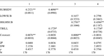
As the G Fund is growing over the course of the sample, first differences were taken of the log of G Fund assets to alleviate concerns about a spurious time trend. Some serial correlation remains in OLS regressions, and this has been addressed by the Cochrane–Orcutt technique. Table 7 presents Cochrane–Orcutt analysis measuring the response of TSP participants to the G Fund subsidy. The dependent variable in each case is the first difference of the log of G Fund assets. SUBSIDY is the yield curve steepness that represents the premium of G Fund interest over money market fund interest. The effect is quite significant, as can be seen in specification 1 – an increase in the subsidy results in an increase in G Fund assets. In specification 2, a control for the money market rate is included, and the coefficient on SUBSIDY remains significantly positive. Comparing the two point estimates, it appears that the subsidy return of the G Fund is a more important attraction to participants than the money market return.
G Fund subsidy and G Fund allocations

Notes: Cochrane–Orcutt procedure to address first-order autocorrelation. Dependent variable is the first difference of the log of G Fund assets. Standard errors in parentheses. Single asterisk denotes 5% significance, double asterisk denotes 1% significance. TBILL (the 3-month Treasury bill rate) and SUBSIDY (the difference between the 10-year Treasury note rate and TBILL) are in decimal. LOWSUB is the minimum of SUBSIDY and its first quartile boundary. HIGHSUB is the difference between SUBSIDY and LOWSUB. The diagnostic statistics include the adjusted R 2, the Durbin–Watson statistic of the transformed equation, the autocorrelation parameter ρ resulting from the Cochrane–Orcutt iterative procedure, and the sample size N.
As discussed in the previous section, portfolio reshuffling might cause this sensitivity to be even greater when the subsidy level is lower. To examine this, SUBSIDY is decomposed as follows:

where LOWSUB is the minimum of SUBSIDY and its first quartile boundary. In other words, LOWSUB captures fluctuations in SUBSIDY between subsidy levels of −0.77% and 0.81% while HIGHSUB captures fluctuations in SUBSIDY above 0.81%. The low-quartile monthly realizations of SUBSIDY are spread across seven of the calendar years of the sample.
These results are presented in the next two columns of Table 7. Contrary to the portfolio reshuffling hypothesis, the G Fund allocation appears more sensitive to fluctuations in the subsidy when the subsidy is high. The difference between the coefficients is not significant, and the results are somewhat sensitive to the threshold between LOWSUB and HIGHSUB, so this difference should not be taken as robust. However, the difference between the two should be significant in the opposite direction for the portfolio reshuffling hypothesis. By failing to support the portfolio reshuffling prediction, these columns present evidence that the G Fund reallocations indeed affect the overall portfolio of the participant.
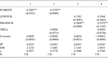
Even in the absence of any new investment by a participant, the G Fund balance will continue to grow due to interest accrual. To control for this, the analysis of Table 7 has been repeated. In Table 8, the dependent variable excludes the estimated effect of accrued interest. That is, the G Fund growth has been reduced by one-twelfth of the annual Treasury note rate. The results validate the overall results shown previously. The point estimates are slightly different, but the statistical significance of the subsidy is very similar to Table 7.
Yield curve and G Fund active allocations

Notes: See notes to Table 7. Dependent variable is the first difference of the log of G Fund assets, net of estimated interest income.
6 The G Fund and Social Security
The TSP has been proposed as a platform for implementing private accounts in a reformed Social Security system. The results presented here have implications for the role of the G Fund in this system. The current system can be used as a benchmark for analyzing investment strategies in a system with private accounts.
The current Social Security system in the United States is a defined benefit plan. Workers' wages are used both as a basis for computing taxes due during work and benefits due upon retirement. Some reform plans, including those endorsed by the President's Commission (2001) and the Administration itself (2005b) involve changing the formula mapping workers wages to benefits. In addition, these plans offer taxpayers the chance to allocate some of their taxes to an individually directed investment account.
If a system without private accounts is used as a benchmark, participating in an individually directed investment account is analogous to investing on margin. At retirement, the taxpayer will have to ‘repay’ the taxes diverted to her account with interest. The interest reflects the opportunity cost to the government of providing the use of the tax revenues. Proposals differ in terms of the opportunity cost used. As an example, the Commission's Plan 2 uses a 2% real interest rate. After the gross value of the redirected taxes is subtracted, the net investment proceedsFootnote 8 are used to purchase additional monthly benefits.
The opportunity cost is calculated using an estimate of the long-term cost of capital to the government, but at retirement no adjustment is made to principal for fluctuations in interest rate. This long-term interest rate without principal fluctuations is of course characteristic of the G Fund. From the taxpayer's point of view, the private account can be thought of as taking a short position in the G Fund and using the proceeds from this short sale to invest in other assets. Seen in this light, allowing the G Fund as an investment option for participating taxpayers effectively represents an opportunity to partially opt-out of the private account by guaranteeing investment income equal to the assessed opportunity cost of capital. The assessed opportunity cost may not exactly equal the G Fund rate, in which case participating also involves an incentive or disincentive to the taxpayer representing the interest differential.
To the extent that G Fund balances are not greater than the tax ‘loan’, then G Fund balances are an opt-out of the system and do not represent a deadweight loss relative to the current system. G Fund balances in excess of the tax loan might represent a deadweight loss. However, since the net investment proceeds must be used to purchase an annuity at retirement, those wishing to avoid risk to their monthly benefit will seek to match the duration of their net portfolio to the the duration of the annuity. For this reason, the F Fund with its positive duration is more attractive than the G Fund with its zero duration.
The fact that the F Fund is less risky in this environment than the G Fund is particularly important, since, for many investors, social security is likely to be their largest financial asset. The Social Security Administration reports (2004) that for one-third of beneficiaries, Social Security represents at least 90% of their income, and for another third, Social Security represents at least half of their income.
In short, Social Security participants are unlikely to take a long position in the G Fund which substantially exceeds their implicit short position in the G Fund. It is beyond the scope of this paper to take a position on the introduction of private investment accounts within Social Security. Including the G Fund in such a plan, however, is unlikely to create the same distortions and deadweight losses experienced within the Thrift Savings Plan. The primary effect of making the G Fund available in a Social Security system is that it effectively allows a partial opt-out of the private investment system. Policymakers may want to decide whether to include the G Fund based on whether they wish to offer this opt-out.
7 Conclusions
This paper has explored the unique nature of the Government Securities Investment Fund (the ‘G Fund’) in the Thrift Savings Plan. The fund provides above-market yields at government expense to the holders of this riskless asset. The offering results in a subsidy of approximately $1 billion annually to federal employees, for whom the G Fund dominates other money market assets.
The availability of this subsidy represents an incentive for federal employees to hold more risk-free assets. These employees have responded by reallocating approximately one-quarter of their balances to the G Fund, while the other three-quarters are allocated similarly to other defined contribution plans. These reallocations are not fully neutralized by external portfolio shifts. The result is that the $1 billion in annual subsidy results in a deadweight loss of up to $400 million per year.
The G Fund would play an important role if it were included in a Social Security private account system. In this case, investing in the G Fund provides a means for investors to partially ‘opt-out’ of the new system.
The G Fund has similarities to stable-value funds offered in private sector defined contribution plans. Further research could examine the welfare implications of these stable value plans. Offering the G Fund amounts to a natural experiment whereby some agents are given access to a higher risk-free rate. This opens up another venue for further research. By observing the elasticity of demand for the risk-free asset, we can learn about the structure of investors' risk aversion. This may cast further light on questions such as the equity premium puzzle.