2. Formulation and solution method

Unless otherwise indicated, in this paper dimensionless units are used with length normalized to Debye length $\lambda _D=\sqrt {\epsilon _0T_0/n_0q_e^{2}}$, velocity to electron thermal speeds $v_{te}=\sqrt {T_0/m_e}$, electric potential to thermal energy $T_0/|q_e|$ and frequency to electron plasma frequency $\omega _{pe}=v_{te}/\lambda _D$ (time normalized to $\omega _{pe}^{-1}$). This normalization reduces the one-dimensional electron Vlasov equation to the form

(2.1)\begin{equation} \frac{\partial f}{\partial t}+v\frac{\partial f}{\partial z}- q_e\frac{\partial \phi}{\partial z}\frac{\partial f}{\partial v} =0. \end{equation}

The ion Vlasov equation is reduced to exactly the same form by using units in which time is measured instead in terms of $\omega _{pi}=\sqrt {m_e/m_i}\;\omega _{pe}$, except that instead of $q_e=-1$ the particle charge for ions is simply reversed $q_i=1$ (so $q\phi$ is the potential energy). Ions in this paper all have mass $m_i=1836m_e$; they are protons.

The formulation and analysis of the electron response follows closely the treatment of previous papers (Hutchinson Reference Hutchinson2018, Reference Hutchinson2019b, Reference Hutchinsona), which should be consulted for the mathematical derivation, including a magnetic field in the $z$ direction. Only an outline description of the method is given here (thus glossing over a large amount of algebraic and numerical work). Vlasov's equation can be integrated along the equilibrium (zeroth order) orbits to obtain the first-order perturbation to the distribution function $f_1$ caused by a first-order electric potential perturbation (relative to the non-uniform hole equilibrium)

(2.2)\begin{equation} \phi_1({{\boldsymbol x}},t)=\hat\phi(z)\exp {\rm i}(ky-\omega t), \end{equation}

(including a perturbation transverse wavevector in the $y$ direction, which for the first three sections of the paper will simply be $k=0$, i.e. one-dimensional variation along the applied uniform magnetic field direction $z$). The integration along unperturbed helical orbits leads to an expansion in (integer $m$) harmonics $\omega _m=m\varOmega +\omega$ of the cyclotron frequency ($\varOmega =eB/m_e$, which represents the magnetic field strength), in which the potential orbit-integrated over earlier time is

(2.3)\begin{equation} \varPhi_m(z,t)\equiv \int_{-\infty}^{t} \hat\phi(z(\tau))\exp({-{\rm i}\omega_m(\tau-t)})\,{\rm d}\tau, \end{equation}

where $z(\tau )=z(t)+\int _t^{\tau } v_z(t')\,{\rm d}t'$ is the orbit position at earlier time $\tau$. For positive imaginary part of $\omega$ the integrals converge and the perturbation in the parallel distribution function (integrated over Maxwellian transverse velocities) then can be found as (see Hutchinson (Reference Hutchinson2018); eq:5.9)

(2.4)\begin{equation} f_{e\parallel 1}(z,y,t) = q_e\phi_1(t)\left.\frac{\partial f_{e\parallel 0}}{\partial W_{e\parallel}}\right|_t \!+\! \sum_{m={-}\infty}^{\infty} {\rm i}\left[\omega_m \frac{\partial f_{e\parallel 0}}{\partial W_{e\parallel}} +(\omega_m-\omega) \frac{f_{e\parallel 0}} {T_\perp}\right] q_e\varPhi_m {\rm e}^{-\zeta_t^{2}}{\rm I}_m(\zeta_t^{2}) {\rm e}^{{\rm i}(ky-\omega t)}, \end{equation}

where $q_e$ is electron charge ($=-1$ in non-dimensionalized units), $W_{e\parallel }$ is the parallel energy $\frac {1}{2}v_z^{2}+q_e\phi$ ($m_e$ being unity), $f_{e\parallel 0}$ is the unperturbed parallel distribution function, a function only of energy and $T_\perp$ is the perpendicular temperature. The parameter $\zeta _t$ is the transverse wavenumber $k$ times the thermal Larmor radius, so that $\zeta _t^{2}=k^{2}T_\perp /\varOmega ^{2}$, and ${\rm I}_m$ is the modified Bessel function. When $\zeta _t$ is small, e.g. because $k$ is small (zero even) or $\varOmega$ is large, then the small-argument Bessel function behaviour (${\rm I}_m(\xi )\to (\xi /2)^{m}/\varGamma (m+1$)) implies that only the $m=0$ cyclotron harmonic is non-negligible. It corresponds to a one-dimensional motion treatment.

The first term of (2.4) is the ‘adiabatic’ perturbation that would arise from a steady potential difference. It does not contribute to the needed response. The remaining harmonic sum is the non-adiabatic contribution denoted $\tilde {f}_{e\parallel }$.

A key formal difficulty is to find the shape of the linearized eigenfunction $\hat \phi (z)$ which self-consistently satisfies the Vlasov and Poisson equations; this is an integro–differential eigenproblem. For slow time dependence relative to particle transit time, it can be argued on general grounds that the eigenmode consists of a spatial shift (by small distance $\xi$ independent of position) of the equilibrium potential profile ($\phi _0$) (see Hutchinson (Reference Hutchinson2018); § 3.1) giving

(2.5)\begin{equation} \hat\phi ={-} \xi \frac{\partial \phi_0}{\partial z}, \end{equation}

which is the perturbation we analyse. Although this is only an approximation to the exact eigenmode, the corresponding eigenvalue of our system can be found to next-order accuracy by using a ‘Rayleigh quotient’ variational approximation (see e.g. Parlett Reference Parlett1974). This mathematical procedure is equivalent to requiring the total force exerted on the particles by the electrostatic field under the influence of the assumed shift eigenmode to equal zero (or to balance the transverse momentum transfer by Maxwell stress if $k\not =0$ – see Hutchinson (Reference Hutchinson2018); § 3). It is the kinematic momentum balance of the electron hole regarded as a rigid composite object. Suppressing the linear $\xi$ factor, the force on the electrons is equal to the force of $\phi _0$ on the non-adiabatic perturbed electron density

(2.6)\begin{equation} \tilde F_e={-}\int\frac{{\rm d}\phi_0}{{\rm d}z}q_e\left( \int \tilde{f}_{e\parallel} \,{\rm d}v_z\right) \,{\rm d}z. \end{equation}

The transverse Maxwell stress force when $k\not =0$ is

(2.7)\begin{equation} F_E \equiv{-}k^{2} \int \frac{{\rm d}\phi_0}{{\rm d}z}\hat\phi\, {\rm d}z , \end{equation}

into which we substitute the shift mode, (2.5 and 2.2).

The essential departure from the previous analysis, required here for slow electron holes, is that the force on the ions cannot be ignored. By the same analysis as the electrons, but substituting ion parameters, that force is

(2.8)\begin{equation} \tilde F_i={-}\int\frac{{\rm d}\phi_0}{{\rm d}z}q_i\left( \int \tilde{f}_{i\parallel}\,{\rm d}v_z\right) \,{\rm d}z, \end{equation}

where

(2.9)\begin{equation} \tilde{f}_{i\parallel} = \sum_{m={-}\infty}^{\infty} {\rm i}\left[\omega_{im} \frac{\partial f_{i\parallel 0}}{\partial W_{i\parallel}} +(\omega_{im}-\omega) \frac{f_{i\parallel 0}}{T_{i\perp}}\right] q_i\varPhi_m {\rm e}^{-\zeta_{it}^{2}}{\rm I}_m(\zeta_{it}^{2}), \end{equation}

with $\varOmega _i=(m_e/m_i)\varOmega$, $\omega _{im}=\omega +m\varOmega _i$ and $\zeta _{it}^{2}=k^{2}T_{i\perp }/\varOmega _i^{2}$. In practice, it is most convenient to calculate the ion force by the same code as the electron force, except reversing the potential sign (as proxy for charge sign), and using a frequency ($\omega$) scaled to be larger by $\sqrt {m_i/m_e}$. Effectively that amounts to solving the ion perturbation in ion scaled units, in which the length scale is the same (using the same reference temperature) and so for the same density we get the same scaled force units.

The specific hole equilibrium potential shape analysed is chosen to be

(2.10)\begin{equation} \phi_0 = \psi \,{\rm sech}^{4}(z/4). \end{equation}

The background (untrapped) electron parallel velocity distribution is taken as an unshifted Maxwellian of temperature $T_0$, and $T_\perp =T_0$. For uniform equilibrium density of ions, the self-consistent equilibrium trapped electron distribution is (Hutchinson Reference Hutchinson2019a) (for negative $W_{e\parallel }$)

(2.11)\begin{equation} f_{t\parallel 0}= f_{e0}\left[\frac{2}{\sqrt{\rm \pi}}\sqrt{-W_{e\parallel}} +\frac{15}{16}\frac{\sqrt{\rm \pi}}{\psi}W_{e\parallel} +\exp({-}W_{e\parallel}){\rm erfc}\left(\sqrt{-W_{e\parallel}}\right)\right], \end{equation}

where $f_{e0}$ is the untrapped electron distribution value at zero energy. It will be shown later that ion equilibrium density non-uniformity gives an adjustment to the trapped electrons, but it is fairly small at relevant $\psi$ for threshold ion distribution shapes.

The background ion parallel velocity distribution is taken as the sum of two Maxwellian components of temperature $T_i$ shifted by $\pm v_s$ and $v_s$ will be stated in units of $\sqrt {T_i/m_i}$. Since ions are repelled by the hole, at some energies one must account for reflection of ions; and the contribution to force will then be different on the two sides of the hole if the ion distribution is asymmetric. Moreover, an equilibrium will exist at only one hole velocity relative to the ion distribution (Hutchinson Reference Hutchinson2021b, Reference Hutchinsona). To avoid having to find the equilibrium, here only symmetric ion distributions $f_i(v)$ will be considered, for which the equilibrium hole velocity is $v_h=0$ and the contributions from the two sides (two incoming ion velocities) to the perturbed $\tilde {f}_i$ are equal.

The numerical calculation proceeds as follows. For a particular $\omega$, the required maximum number of cyclotron harmonics is found, based on $\zeta _t$; then for each cyclotron harmonic $m$ the integrals over $z$ and equivalently $\tau$ of (2.3), and then (2.6) or (2.8) are carried out numerically for fixed $W_\parallel$ (and ${\rm d}W_\parallel =v_z\,{\rm d}v_z$ so that the phase-space element ${\rm d}v_z\,{\rm d}z\to {\rm d}W_\parallel \,{\rm d}\tau$). It proves more accurate to integrate (2.3) as it stands, rather than first analytically integrating by parts as was previously done (Hutchinson Reference Hutchinson2018). This improvement is especially important for the ion calculation, in which the frequency of interest is high relative to the bounce and transit frequencies. After multiplying $v_z\,{\rm d}v_z\int \varPhi _m \,{\rm d}z$ by the terms $\omega _{m}({\partial f_\parallel }/{\partial W_\parallel })$ and $(\omega _m-\omega )f_\parallel$, the resulting ${\rm d}F$, when divided by ${\rm d}v_z$ gives the differential contribution to force per unit $v_z$ which is denoted ${{\rm d}F}/{{\rm d}v}$.

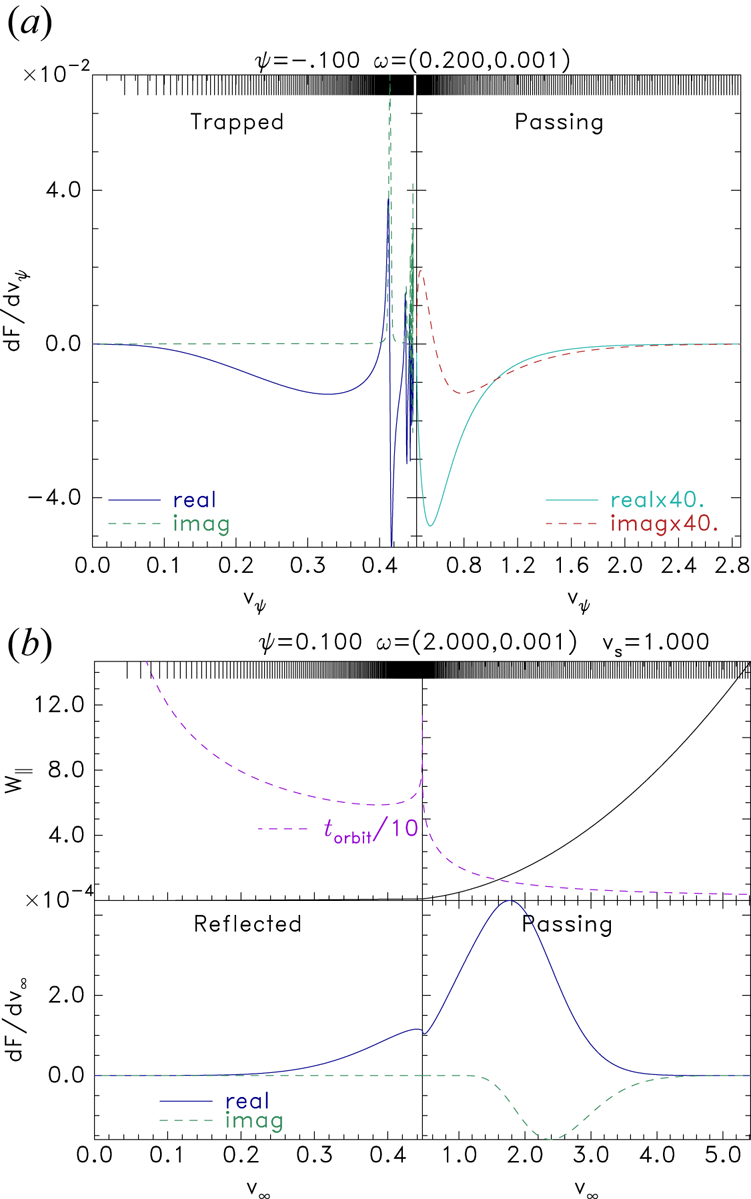
In figure 1 are shown illustrative cases of ${{\rm d}F}/{{\rm d}v}$ as a function of $v_z$, for $k=0$ ($m=0$). We observe that the attracted species force (figure 1a) is dominated by the trapped particles, the (single Maxwellian) passing contribution being practically negligible. Near the trapped–passing boundary ($W_\parallel =0$ where $v_\psi =\sqrt {2\psi }$) oscillations require fine mesh spacing to resolve, but their contribution is not strong because of the limited extent in $v_\psi$ and significant cancellation. By contrast, the repelled species (figure 1b), normally ions, (whose plotted parameters are normalized to the ion thermal speed and plasma frequency) for which higher frequencies are dominant, has no such oscillations. However, its resolution challenges lie in the oscillations during integration of $\varPhi _m$ on the spatial mesh, which are not visible in this plot. For this repelled species the time duration $t_{{\rm orbit}}$ of the orbit (to travel from and back to the chosen integration boundary) has a cusp at marginal reflection, and becomes very long for reflected orbits at lower energy, which dwell near reflection. The resulting averaging over fast $\phi _1$ time oscillations rapidly suppresses the perturbed force; and so passing orbit contributions dominate.

Figure 1.

Illustration of the contributions to force ${\rm d}F/{\rm d}v$ as a function of parallel velocity. (a) For the attracted species, as a function of $v_\psi$, the velocity at the hole centre $\phi =\psi$. Orbits are trapped for $v_\psi <\sqrt {2|\psi |}$. Note that passing force has been multiplied by 30 for visibility; so it is small, and its velocity axis scale is also different. (b) For the repelled species as a function of the distant velocity $v_\infty$, in which the upper subpanels show the energy and the orbit duration $t_{{\rm orbit}}$. The non-uniform velocity integration mesh used is indicated at the top of each plot.

To get the total force for the entire velocity distribution, ${{\rm d}F}/{{\rm d}v}$ is multiplied by the ${\rm I}_m(\zeta _t)$, and summed over relevant harmonics $m$. This process is mathematically equivalent to integrating over perpendicular distribution for low magnetic field, but for $\zeta _t\to 0$ requires only $m=0$, the perpendicular Maxwellian integration having been transferred to the Bessel function. In this section and the next we show results only for this limit (effectively $k=0$). We arrive at the total particle force $\tilde F$ exerted by the potential, at this chosen $\omega$. 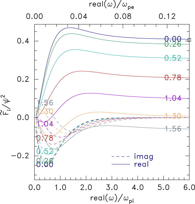The complex ion force $\tilde F_i$ as a function of real frequency (strictly for small positive imaginary part of $\omega$) is plotted in figure 2, normalized to $\psi ^{2}$ the hole potential amplitude squared, which is the dominant scaling. The tendency to a real constant value at high frequency is because the ion charge density remains stationary when the potential shifts faster than the ions can respond ($\omega \gg \omega _{pi}$). The reversal of the value with ion distribution shape ($v_s$) is because $f_{i\parallel }(v_z)$ develops a local minimum at $v=0$ when the velocity shift of the components is more than ${\sim }1.1$. This is approximately the shape at which exponential instability ceases. A way to understand the force reversal intuitively is that the ion density in equilibrium becomes larger in the positive potential hole than outside it, rather than being smaller for a low shift (e.g. Maxwellian, $v_s=0$). A positive equilibrium ion density deviation is repelled by the shifted potential, and the result tends to oppose the shift of the hole (recognizing that the hole has effectively negative inertia Hutchinson (Reference Hutchinson2019a)). The algebra quantifies this intuition.

Figure 2.

The real and imaginary parts of the ion force as a function of real $\omega$ for several different values of $v_s$ labelling the curves. At high frequency, the force for an effectively immobile Maxwellian distribution $v_s=0$ is shown by the square point, and agrees with the corresponding numerical integration line. The plot is independent of the value of hole amplitude $\psi$ when it is small (0.001 here).

In figure 2, a square at the right-hand side of the plot represents the analytic value $F_i=(128/315)\psi ^{2}$ of the ion force for a small amplitude $\,{\rm sech}^{4}$ shape hole and Maxwellian ions immobile on the time scale of the shift perturbation. Its agreement with the numerical calculation at $v_s=0$ is one of the verification tests of the code. Another is that independent numerical calculation shows (reference Hutchinson (Reference Hutchinson2021b); figure 2) that the immobile-ion force is zero for small $\psi$ at $v_s=1.3$, which is also in agreement with figure 2. Verification of the passing and trapped force code for the attracted species consists of a detailed quantitative comparison of the new code's force results with equivalent calculations from the independent prior code, whose results have been compared with analytic estimates (Hutchinson Reference Hutchinson2019a) and PIC calculations (Hutchinson Reference Hutchinson2019b), as well as agreement with the analytic electron force at very high frequency where even electrons are immobile;

(2.12)\begin{equation} \left(\tilde F_e\to -\left(\frac{128}{35}-\frac{512}{63}+\frac{3200}{693}\right) \psi^{2}={-}0.14776\psi^{2}\right). \end{equation}

There is an important adjustment in the electron force that arises, particularly for peaked ion distributions ($v_s\lesssim 0.5$). It is that the ion depletion contribution to the equilibrium charge changes the required equilibrium trapped electron depletion and thus changes $\partial f_{e\parallel 0}/{\partial W_{e\parallel }}$ for fixed $\phi (z)$. The effect is conveniently accounted for by scaling the electron depletion, i.e. the difference between the trapped distribution and a flat distribution $f_{e\parallel 0}-f_{e0}$ (2.11), by a single factor we shall write as $1+c_i$, where $c_i$ is proportional to the ion equilibrium density non-uniformity, and is independent of $W_\parallel$. A fit to the ion response previously found (Hutchinson Reference Hutchinson2021b) provides the value of $c_i$.Footnote ¹ The factor $1+c_i$ approximately doubles $f_{e\parallel 0}-f_{e0}$ at zero $v_s$, passes through unity near $v_s=1.2$, and remains near 0.8 for higher $v_s$. This approximation of the ion equilibrium effects introduces uncertainties that are no greater than those implied by the adoption of the $\,{\rm sech}^{4}$ potential form in the first place, and by the assumption that the eigenmode is the shift mode.

The force-balance dispersion relation,

(2.13)\begin{equation} (\tilde F\equiv)\tilde F_e+\tilde F_i=F_E, \end{equation}

which is a complex equation requiring both real and imaginary parts to be zero, is not satisfied by an arbitrary complex $\omega$. The $\omega$ that does satisfy it (if any), can be found either by contouring in the complex $\omega$ plane the real and imaginary parts of $\tilde F-F_E$ and finding where their zero contours cross, or by two-dimensional Newton iteration to find the complex root of $\tilde F-F_E$ (constrained by requiring ${{\rm Re}}(\omega )\ge 0$ and ${{\rm Im}}(\omega )\ge 0$).

3. One-dimensional stability: mechanism and results

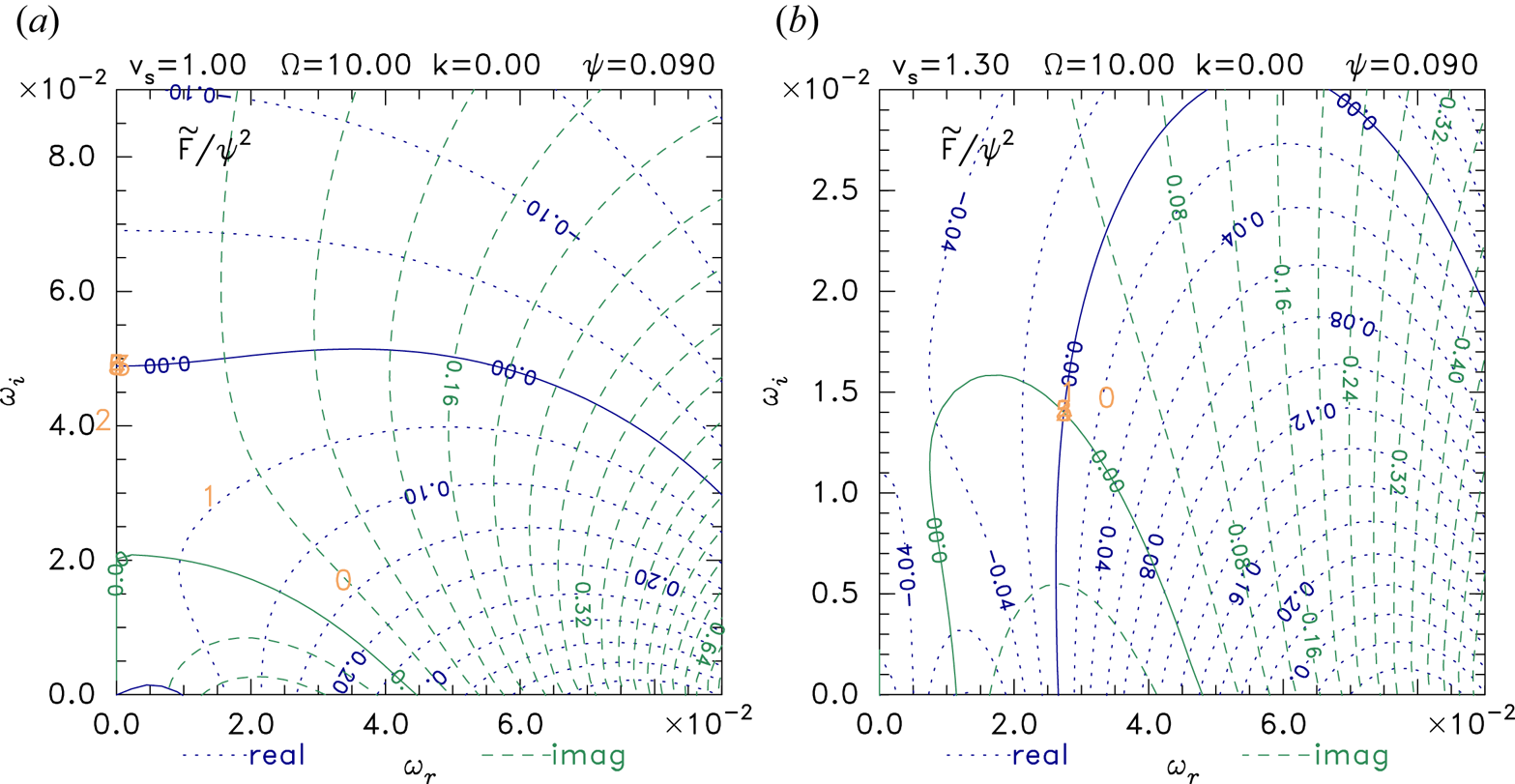
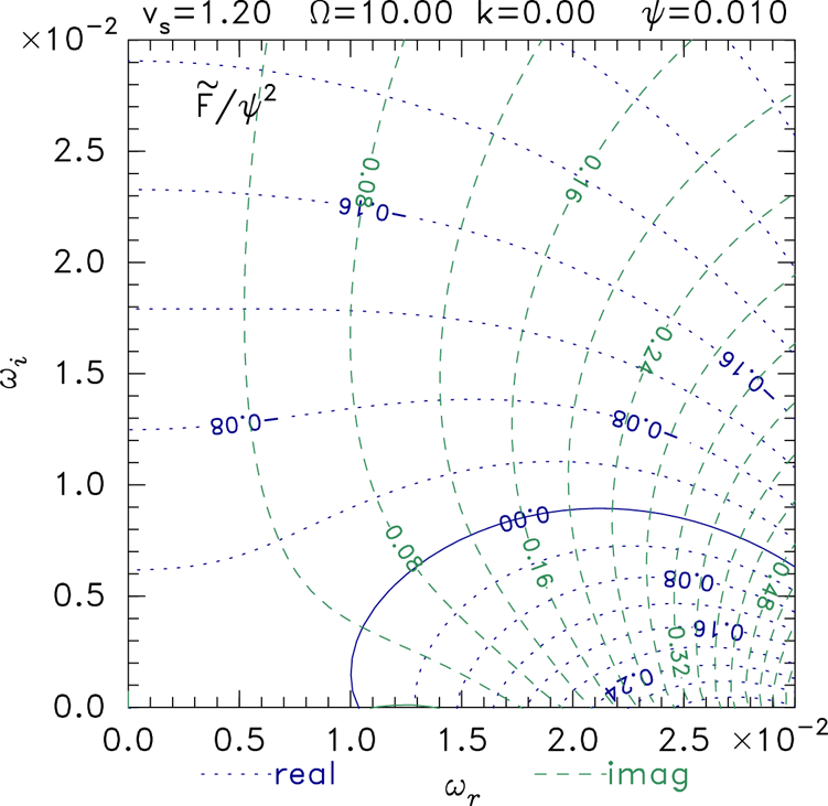
In this section we presume $k=0$, which means $F_E=0$ and motion is effectively one-dimensional. Figure 3 shows example contour plots of the total complex force in the complex $\omega$ plane. The complex root of the dispersion relation is where $\tilde F=0$, at the intersection of the zero contours of its real and imaginary parts. At $v_s=1$ (figure 3a), where there is no local minimum in the ion velocity distribution, a purely exponentially growing instability occurs at $\omega \simeq 0.05{\rm i}$. At $v_s=1.3$ (figure 3b), where a local minimum is present, the root is a slower-growing oscillation $\omega \simeq 0.028+0.014{\rm i}$. This second type of solution was unaddressed in the prior slow hole stability analysis.

Figure 3.

Contours of real and imaginary parts of total force $\tilde F$ over the relevant complex $\omega$ region. Solid contours have value zero. The sequence of (orange) numbers on the plane show where Newton iterations (starting at 0) take the iterative solution. It converges at the intersection of the zero contours, where $\tilde F=0$. In (a) $v_s=1$, the solution lies on the ${{\rm Re}}(\omega )=0$ boundary, where ${{\rm Im}}(\tilde F)=0$. In (b) with larger ion component separation $v_s=1.3$, there is no solution with ${{\rm Re}}(\omega )=0$, but a slower growing oscillation occurs at finite ${{\rm Re}}(\omega )$.

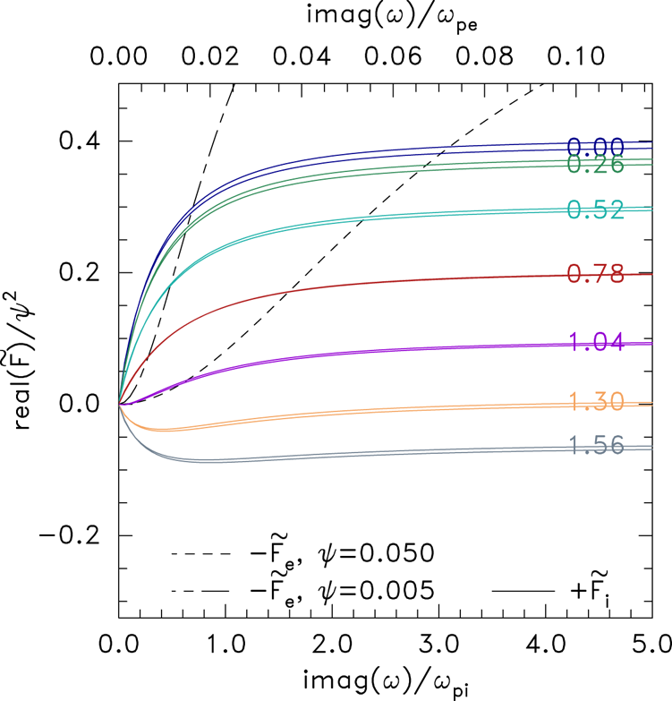
The disappearance of the purely growing mode can be understood by plotting the ion and electron forces along the ${{\rm Re}}(\omega )=0$ boundary. As shown in figure 4, although the ion force normalized to $\psi ^{2}$ is very insensitive to the $\psi$ value, that is not true of the electron force. The reason is that $F_e$ mostly comes from trapped particles whose bounce frequency is $\omega _b\propto \sqrt {\psi }$, and $\omega _b/\omega$ determines the force variation. By contrast, the ion force is predominantly passing (no ion trapping), and has much weaker scaled dependence on $\psi$. When $v_s\gtrsim 1$ no intersection ($\tilde F_i=-\tilde F_e$) occurs for small enough $\psi$, and there is no instability having ${{\rm Re}}(\omega )=0$. All this is consistent with the previously published slow hole stability analysis concentrating on the high and negligible real frequency regions of the $\omega$ plane, which concluded that a local minimum in $f_i(v)$ was necessary for stability.

Figure 4.

Scaled force $\tilde F/\psi ^{2}$ as a function of purely imaginary $\omega$. The ion force $\tilde F_i$ is almost independent of $\psi$ but depends on $v_s$ shown by labels on the solid lines. The dashed curves give minus the electron force for the different $\psi$ values. A growing mode requires $\tilde F_i=-\tilde F_e$: an intersection. When $v_s$ is large enough, there are no intersections.

However, the oscillatory solution of figure 3(b) can remain even when there is a local $f_i$ minimum if the ${{\rm Im}}(\tilde F)=0$ contour lies above the real $\omega$-axis. The solution disappears if the hole amplitude is small enough, because the ${{\rm Im}}(\tilde F)=0$ contour disappears below the real axis, as figure 5 illustrates. The root itself, where ${{\rm Re}}(\tilde F)=0$ is zero as well as ${{\rm Im}}(\tilde F)$, likewise disappears. The case shown has just sufficiently low $\psi$ for total stability. Newton iterations bump up against the ${{\rm Im}}(\omega )\ge 0$ constraint without finding a zero. Decreasing $\psi$ or increasing $v_s$ moves the (barely visible) imaginary contour even farther down out of the unstable domain.

Figure 5.

Force contours for a stable case at small $\psi$ with sufficient ion component shift to give a local minimum. The negative imaginary contour is disappearing below the real axis removing the root of $\tilde F$ from the unstable domain.

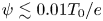
Thus, there are really two requirements for the slow electron hole to be fully stable, to oscillatory as well as purely growing modes: (A) that there be a local minimum in the ion distribution $f_i(v)$ ($v_s\gtrsim 1.1 v_{ti}$); and (B) that the hole's potential amplitude $\psi$ should be small enough ($\psi \lesssim 0.01 T_e/e$).

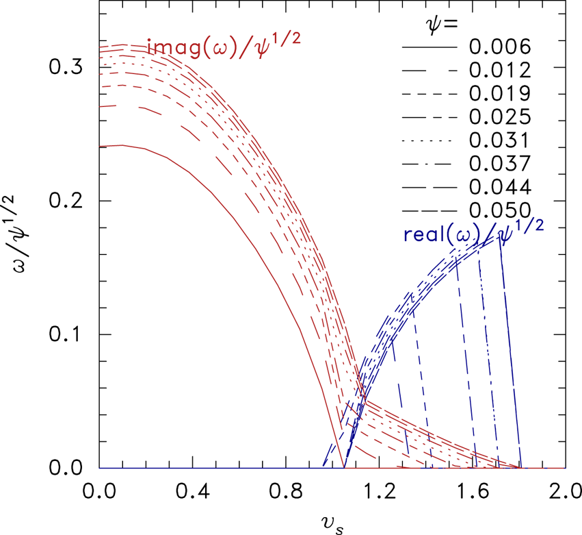
More quantitatively, a range of results is summarized in figure 6. At low $v_s$, the shift mode is purely growing, with a scaled rate ${{\rm Im}}(\omega )\simeq 0.3\psi ^{1/2}$ for a Maxwellian ($v_s=0$) ion distribution. The transition to oscillation occurs close to $v_s=1$, and the growth rate ${{\rm Im}}(\omega )$ decreases quickly (as the local minimum of $f_i(v)$ develops) by a total factor of approximately 10. As that minimum deepens ($v_s$ increasing further), the growth rate drops more slowly and the oscillation frequency ${{\rm Re}}(\omega )$ increases until at a depth dependent on $\psi$ the growth becomes zero and the instability disappears. If the amplitude is small enough $\psi \lesssim 0.01$, there is no oscillatory instability, and developing a local bare minimum in $f_i$ is sufficient for stability.

Figure 6.

The real and imaginary parts of unstable mode frequency versus ion distribution shape ($v_s$), for a range of peak potential amplitudes ($\psi$).

4. Variation with other parameters

4.1. Ion temperature

When ion temperature $T_i$ is different from electron temperature ($=T_0$), the ion force is changed. Referring to (2.8) and (2.9), the quantities that are directly affected are ${\partial f_{i\parallel 0}}/{{\rm d}W_{i\parallel }}$, ${f_{i\parallel 0}}/{T_{i\perp }}$ and $\zeta _{it}$. In this subsection we will not address $\zeta _{it}$ changes with $T_i$. They give negligible effect in the strong ($\zeta _t\to 0$) and weak ($\zeta _t>20$) magnetic field limits. For simplicity supposing the two parallel-shifted Maxwellian ion components remain isotropic, the effect of $T_i$ changes on ${\partial f_{i\parallel 0}}/{{\rm d}W_{i\parallel }}$ and ${f_{i\parallel 0}}/{T_{i\perp }}$ is to divide the ion force by $T_{i}/T_0$; because the changes arising from $f_{i\parallel 0}$ itself (reducing its height $\propto 1/\sqrt {T_i}$, and increasing its velocity width $\propto \sqrt {T_i}$), cancel each other out. Thus, the ion density perturbations, both in equilibrium and resulting from $\phi _1$, are multiplied by $T_0/T_i$. And since we are citing $v_s$ in ion thermal units, the ion velocity distribution relative shape is independent of $T_i$. Therefore, ion temperature can be accounted for by multiplying the ion force $\tilde F_i$ and the equilibrium ion density non-uniformity by $1/T_i$.

Because the equilibrium ion density is changed by $T_i$, the electron force is also changed indirectly by adjustment of the required electron trapped distribution for equilibrium. The trapped electron equilibrium deficit is proportional to $(1+c_i/T_i)$ and the electron force is scaled by the same factor, which varies more slowly than the ion force factor $1/T_i$.

Higher ion temperature therefore decreases the force on the ions relative to that on the electrons. Referring back to figure 4, the different scaling of these curves has the effect of moving the intersection $\tilde F_i=-\tilde F_e$ to lower imaginary values of frequency, that is of reducing the growth rate, as $T_i$ increases.

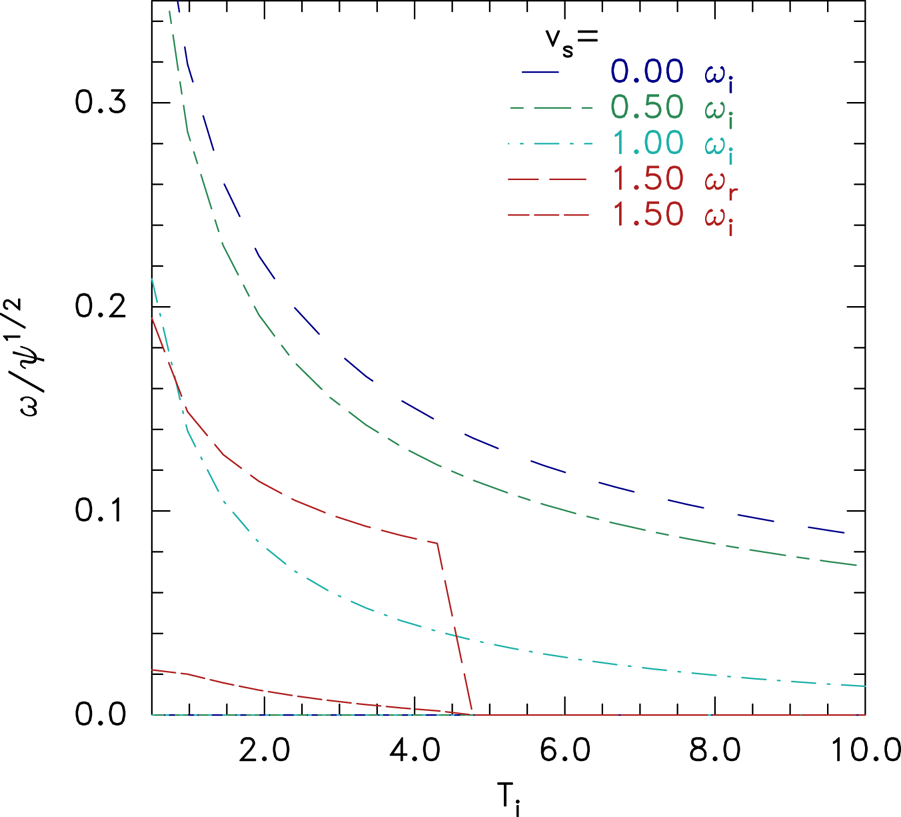
Figure 7 illustrates the resulting variation of the instability frequency found by full numerical integration for $k=0$. Increasing $T_i$ always decreases the growth rate. For $v_s\lesssim 1.1$ the real frequency is zero, and is not plotted. For the oscillatory instability regime, $v_s\gtrsim 1.1$, increasing $T_i$ can lead to a full stabilization: when $\psi =0.05$ and $v_s=1.5$ at $T_i\simeq 5$.

Figure 7.

Variation of unstable frequencies ($\omega _i$ imaginary, $\omega _r$ real if non-zero) with ion temperature, for different $v_s$. Here $\psi =0.05$.

4.2. Transverse variation: multidimensional instability

Multidimensional instability here means situations in which although the equilibrium is independent of transverse position, the perturbation varies transversely: $k\not =0$. And in this section we shall suppose that the magnetic field is strong enough that still only the $m=0$ cyclotron harmonic matters because $\zeta _t$ remains small. In that case the only new effect is that the transverse Maxwell stress force $F_E$ (2.7) is non-zero and must be included in the dispersion equation (2.13). Again suppressing the linear $\xi$ factor, for the shift mode, it becomes

(4.1)\begin{equation} F_E= k^{2}\int\left(\frac{{\rm d}\phi_0}{{\rm d}z}\right)^{2}\,{\rm d}z= k^{2} \frac{128\psi^{2}}{315}, \end{equation}

where the final equality applies for the specific $\,{\rm sech}^{4}$ potential shape. Therefore, if we consider the transverse wavenumber $k$ to be an arbitrary (real) choice, then we must examine the effect of including an $F_E$ that is real and positive, but of arbitrary magnitude. Thus, we must allow the real part of $\tilde F$ to be positive.

The contour plots of figure 3 (for example) allow us immediately to deduce what happens to the unstable root as $F_E$ increases from zero: it becomes the intersection of the unchanged solid ${{\rm Im}}(\tilde F)=0$ contour with a different real contour ${{\rm Re}}(\tilde F)=F_E$, instead of zero. For example, in the case of figure 3(a) if a value $F_E=0.1\psi ^{2}$ is included, the relevant real contour is the one labelled 0.1. The root is then instead at $\omega \simeq (2.4+1.5{\rm i})\times 10^{-2}$, giving a slower growing oscillatory instability rather than the purely growing one for $k=0$. By (4.1) $F_E/\psi ^{2}=0.1$ corresponds to $k=\sqrt {0.1\times 315/128}=0.496$, which is at the limit of high $k$, short wavelength; smaller $k$ values will have even less effect.

Similarly in figure 3(b) as $k$ is increased, the relevant real contour moves to the right, and the root to higher real and lower imaginary frequency. For the case of figure 5, the motion of the real contour to the right can give the root a slightly positive imaginary frequency, and so induce a very slow instability where there was none before. But further increase of $k$ brings the intersection past the region ($1.1<\omega _r<1.3$) where the imaginary contour is positive, thus restabilising it.

To summarize, finite $F_E$ arising from non-zero $k$ always acts in such a direction as to make purely growing instabilities more stable, and usually does so even for oscillatory modes. We therefore do not expend further effort here to quantify in separate detail $F_E$-effects because almost always the $F_E=0$ situation already treated is the most unstable. Nevertheless $F_E$ is fully included in the results of the following section.

4.3. Magnetic field strength

When $k\not =0$ and $\varOmega$ is not very large, the Bessel function argument may not be small, and the sum over harmonics $m$ may include many relevant terms. In this regime, the stability can depend on the magnetic field strength. Since the ion thermal Larmor radius $r_L$ is greater than the electron by a factor $\sqrt {m_i/m_e}$ (for comparable temperature), the ions will generally experience $\zeta _t(=kr_{L})\gtrsim 1$ first. The number of harmonics making significant contribution, when substantially greater than one, may be estimated by noting that $\zeta _t{\rm e}^{-\zeta _t^{2}}{\rm I}_m(\zeta _t^{2})$, regarded as a function of integer $m$, is approximately a Gaussian ${\rm e}^{-v_m^{2}/2}/\sqrt {2{\rm \pi} }$, where $v_m=m/\zeta _t$. We therefore require contributions up to $v_m\sim 3$, i.e. $m\sim 3\zeta _t$. However, with this velocity identification, $\omega _m=\omega +m\varOmega =\omega +kv_m$, so writing ${\rm d}v_m=1/\zeta _t=\varOmega /k$, (2.9) becomes

(4.2)\begin{align} &\sum_{m={-}\infty}^{\infty} {\rm i}\left[\omega_{m} \frac{\partial f_{{\parallel} 0}}{\partial W_{{\parallel}}} +(\omega_{m}-\omega) \frac{f_{{\parallel} 0}}{T_{{\perp}}}\right] q\varPhi_m {\rm e}^{-\zeta_{t}^{2}}{\rm I}_m(\zeta_{t}^{2})\nonumber\\ &\quad \simeq \sum_{m={-}\infty}^{\infty} {\rm i}\left[(\omega+kv_m) \frac{\partial f_{{\parallel} 0}}{\partial W_{{\parallel}}} +kv_m \frac{f_{{\parallel} 0}}{T_{{\perp}}}\right] q\varPhi_0(\omega+kv_m){\rm e}^{{-}v_m^{2}/2}\,{\rm d}v_m. \end{align}

The second form is a finite difference approximation of the unmagnetized integral expression: $\sum _{m=-\infty }^{\infty } \,{\rm d}v_m\simeq \int _{-\infty }^{\infty } \,{\rm d}v$. Thus, as physical considerations dictate, the limit of small $\varOmega /kv_t$ gives simply an unmagnetized integral over the $k$-component of the perpendicular velocity distribution. This is often the case for the ions.

Although the numerical routineFootnote ² evaluating the higher-order Bessel functions (by backward recurrence) works well only up to approximately ${\rm I}_{60}$, a maximum value of $|m|=60$ is sufficient for the harmonic sum to represent the integral limit very well. It is then effectively already in the zero field limit. Therefore, the present evaluation of $\tilde {f}$ does not bother to switch to a higher-resolution finite-difference integral representation, and instead artificially limits how small an $\varOmega$ is permitted, and uses (4.2) with an effective value of $\varOmega$ no smaller than that which requires a maximum $|m|\le 60$, i.e. $\zeta _t\lesssim 20$. (The required effective $\varOmega$ lower limit is different for electrons and ions.)

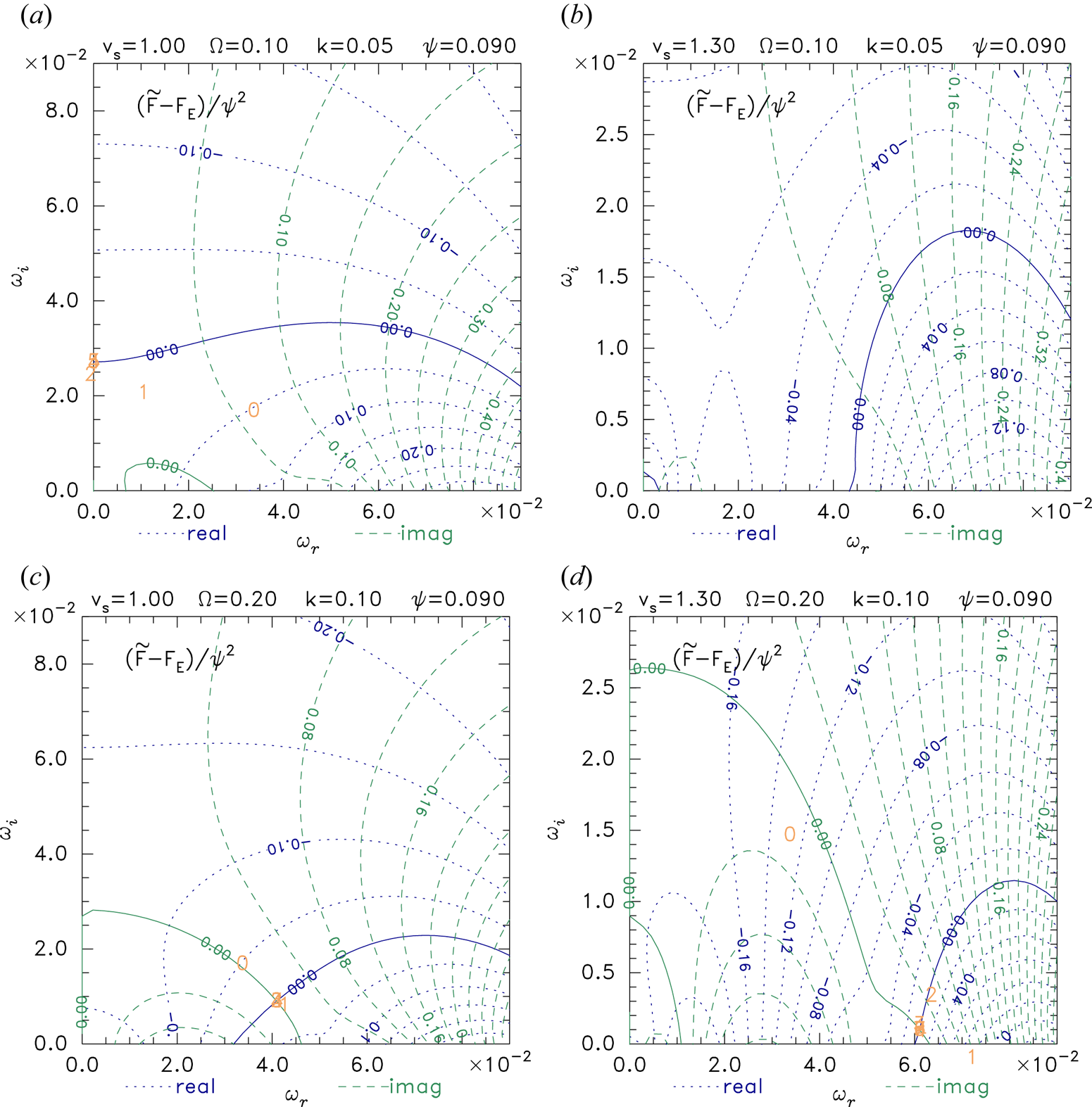
Figure 8 shows the effect of non-zero $k$ and $\varOmega =2k$ on the cases of figure 3, with which it should be compared. Figure 8(a,b) have $k=0.05$ and show mostly a movement of the contours downward towards a more negative imaginary part ($\omega _i$) of $\omega$. Figure 8(a) has a relatively small growth rate reduction; but figure 8(b), which has a local $f_i$ minimum, shows complete stabilization of the prior unstable oscillatory mode. Figure 8(c,d) have the same ratio $\varOmega /k$ as figure 8(a,b) but twice as large values: $k=0.1$. In figure 8(c) the mode oscillates with real frequency $\omega _r\simeq 0.04$. In figure 8(d) there is again tendency to higher real frequency, compared with figure 3, but a very slow growing oscillatory instability remains, unlike figure 8(b) which was fully stabilized. The differences between figure 8(a) and figure 8(c) and between figure 8(b) and figure 8(d) are practically all differences in the electron force $\tilde F_e$, with a modest contribution from $F_E$ differences. There is essentially negligible change in $\tilde F_i$, because $\zeta _t$ is so large that we are in regime of quasi-continuous perpendicular integration, and the value of $kv_{ti}$, much smaller than typical $\omega$, gives little effect.

Figure 8.

Force contours with non-zero $k$ and low enough $\varOmega$ to affect stablity.

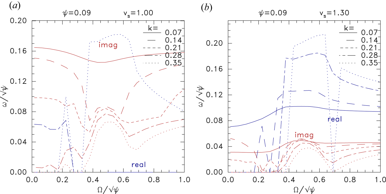
Figure 9 shows the real and imaginary parts of the dispersion solution $\omega$ as a function of magnetic field strength $\varOmega$. The different $k$ values control the strength of the effect of transverse variation. The lowest $k=0.07$ value (solid lines) shows rather weak variation from the $k=0$ case (not shown) which gives a solution independent of $\varOmega$ and equal to the high-$\varOmega$ limit of the solid lines. In figure 9(a) the single-humped ion velocity distribution gives a purely growing mode (${{\rm Re}}(\omega )=0$) at low $k$ (0.07 and below) with growth rate approximately 0.16. All higher $k$ values have growth rates smaller than this. Some of them make transitions to oscillatory (${{\rm Re}}(\omega )\not =0$) modes in the middle of the $\varOmega$ range, with growth rates typically half as great. In figure 9(b) for a double-humped ion distribution, similar trends are evident, but the growth rate is considerably smaller $\lesssim 0.05$, and the real frequency never reverts to zero at high $\varOmega$, consistent with the previous observation that for such distributions one-dimensional modes are all oscillatory, and are unstable at this $\psi$ value.

Figure 9.

Dependence of the real and imaginary parts of the instability frequency on magnetic field strength, $\varOmega$, for a range of transverse wavenumbers $k$. (a) Single humped $f_i(v)$ $v_s=1$ ; (b) double-humped $v_s=1.3$, for a moderately deep hole $\psi =0.09$.

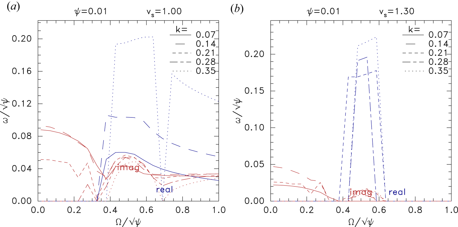
At smaller potential amplitude, figure 10, the double humped $v_s=1.3$ case (figure 10b) looks very different. It is stable for $\varOmega /\sqrt {\psi }\gtrsim 0.65$ for all $k$ values, consistent with figure 6. An oscillatory instability of low growth rate exists in the range $0.4\lesssim \varOmega /\sqrt {\psi }\lesssim 0.65$ except at very low $k$, and a purely growing mode below 0.4 for several $k$ values. In fact this plot looks extremely similar to figure 3 of Hutchinson (Reference Hutchinson2019b), concerning transverse instability of fast electron holes with zero ion force. That is a sign that this instability is driven by the electrons with little contribution from the ions. It is effectively a slightly modified fast hole transverse instability. Figure 10(a) with single humped ion distribution, by contrast, has unstable oscillatory solutions all the way out to large $\varOmega$. These are driven by the combined electron and ion response, and are limited to slow holes. The low $\varOmega$ part of this plot has a character more like figure 10(b) than figure 9(a), and might be thought of as the transverse instability modified by the slow hole ion response.

Figure 10.

As in figure 9, except for smaller potential amplitude $\psi =0.01$.

5. Summary

Slow electron holes are subject to instability of their velocity because of interaction with bulk ions. The purely growing one-dimensional ($k=0$) instability disappears when a local minimum exists in the ion velocity distribution ($v_s\gtrsim 1.1v_{ti}$ for symmetric Maxwellian ion beams), in accordance with earlier studies. However, an oscillatory instability (overstability) remains up to relatively deep local minima, depending on the potential amplitude $\psi$ of the equilibrium, as shown in figure 6. Its growth rate is much smaller than the purely growing mode. If the peak hole potential $\psi$ is less than approximately $0.01T_e/e$ (for $T_i=T_e$ but larger for larger $T_i$ – see figure 7), the overstability disappears, this favours stability of low amplitude slow electron holes, which seems consistent with several observational studies (Kamaletdinov et al. Reference Kamaletdinov, Hutchinson, Vasko, Artemyev, Lotekar and Mozer2021).

When, $k\not =0$, instabilities of slow holes have generally lower growth rate than when $k=0$, except that when $(\varOmega /\omega _{pe})/\sqrt {e\psi /T_e}\lesssim 0.6$ even low amplitude holes experience transverse instability driven predominantly by the electron response and not much affected by ion coupling. Its real frequency becomes zero if $(\varOmega /\omega _{pe})/\sqrt {e\psi /T_e}\lesssim 0.4$.

An overall caveat to the present work is that it has analysed only the pure shift mode. Under some circumstances a distorted shift can become more unstable (Hutchinson Reference Hutchinson2019b). This might modify the exact values of the instability thresholds.

The observational implications of the current results are broadly these. Slow electron holes in single humped background ion distributions will speed up without oscillations with growth time of order $0.3/(\psi ^{1/2}\omega _{pe})$. They are predicted to remain slow for only a few growth times. By contrast, when $f_i$ has a local minimum in which the hole speed lies, the oscillatory instability growth time is longer by a factor of order 10; so they remain slow at least that much longer. The oscillation real angular frequency is of order $0.1\psi ^{1/2}\omega _{pe}$. When the hole potential is smaller or the $f_i$ local minimum deeper, the growth rate of one-dimensional modes eventually becomes zero, unless the magnetic field is low enough that the electron transverse instability is excited. Therefore, the oscillatory instability discovered here can be avoided entirely in plausible parameter regimes. Furthermore, slow holes might be observed soon after formation even in regimes that have slowly growing instabilities.

It would be of considerable interest to verify by simulation the results of the present study. The required simulations for detailed quantitative comparison are rather difficult because they need a fully self-consistent steady slow hole initial equilibrium. My preliminary efforts, using hole potentials $\psi$ considerably larger (0.2–0.4) than those for which this analysis predicts stability, do show oscillatory instabilities which are broadly consistent with present theory – in that they are shift modes in approximately the right frequency range: ${{\rm Re}}(\omega )/\psi ^{1/2}\sim 0.1/\omega _{pe}$. However, the computational cost of simulations with sufficient signal-to-noise or velocity resolution increases rapidly with decreasing $\psi$, and have not yet been carried out in the lower-$\psi$ stabilized regime.