1 Introduction
Smooth-wall turbulent flows exhibit a structural paradigm wherein the flow is occupied by an inner and outer cycle, the former being associated with the viscous-affected near-wall region while the latter is associated with large-scale, meandering zones of momentum excesses and deficits known as large-scale motions (LSM) (Hutchins & Marusic Reference Hutchins and Marusic2007a
,Reference Hutchins and Marusic
b
). LSMs are attributed to packets of hairpin vortices that occur in streamwise succession, have similar propagation speeds and increase in size in the streamwise direction (Adrian Reference Adrian2007). In this document, the first, second, and third component of any vector,
 $\boldsymbol{x}=\{x_{1},x_{2},x_{3}\}$
, corresponds to its magnitude in the streamwise (
 $x_{1}$
), spanwise (
 $x_{2}$
) and wall-normal direction (
 $x_{3}$
), respectively; superscript prime denotes fluctuation about the Reynolds average (unless noted otherwise),
 $\boldsymbol{x}^{\prime }=\boldsymbol{x}-\langle \boldsymbol{x}\rangle _{T}$
; and tensors are denoted via bold sans relief, i.e.
 $\unicode[STIX]{x1D653}=\boldsymbol{x}\otimes \boldsymbol{x}$
, while tensor constituents are denoted by sans relief followed by numerical indices corresponding to those used for a vector, i.e.
 $\unicode[STIX]{x1D61F}_{12}$
for the streamwise–spanwise component. At yet larger scales, LSMs undergo a streamwise coalescence to form very-large-scale motions (VLSM) (Kim & Adrian Reference Kim and Adrian1999; Balakumar & Adrian Reference Balakumar and Adrian2007; Hutchins & Marusic Reference Hutchins and Marusic2007a
; Dennis & Nickels Reference Dennis and Nickels2011a
,Reference Dennis and Nickels
b
). The nature, and, indeed, the existence of structures in the inner and outer layer is predicated upon inertial conditions, where friction Reynolds number,
 $Re_{\unicode[STIX]{x1D70F}}=u_{\unicode[STIX]{x1D70F}}\unicode[STIX]{x1D6FF}\unicode[STIX]{x1D708}^{-1}$
, is a commonly used measure of flow state (
 $u_{\unicode[STIX]{x1D70F}}$
and
 $\unicode[STIX]{x1D708}$
represent shear velocity and kinematic viscosity, respectively).
 $Re_{\unicode[STIX]{x1D70F}}\gtrsim 2000$
is a commonly cited threshold condition for the formation and sustenance of outer-layer LSMs (Hutchins & Marusic Reference Hutchins and Marusic2007a
) and fully rough conditions (Antonia Reference Antonia1981; Krogstad, Antonia & Browne Reference Krogstad, Antonia and Browne1992; Jimenez Reference Jimenez2004; Schultz Reference Schultz2007; Schultz & Flack Reference Schultz and Flack2009; Flack & Schultz Reference Flack and Schultz2010). Moreover,
 $Re_{\unicode[STIX]{x1D70F}}$
is also helpful for designating the regimes over which different flow analysis schemes may be used.
Roughness ablates the inner layer – leaving in its place the so-called roughness sublayer – and induces a momentum deficit of the outer flow known as the roughness function,
 $\unicode[STIX]{x0394}U^{+}$
. Turbulence within the roughness sublayer is characterized by coherent structures with geometric macroscale of the order of individual roughness element height,
 $h$
(Castro Reference Castro2007). The roughness sublayer depth,
 $x_{3,RSL}$
, scales linearly with
 $h$
, and a consensus range is generally
 $2\lesssim x_{3,RSL}/h\lesssim 5$
(Grass Reference Grass1971; Raupach, Antonia & Rajagopalan Reference Raupach, Antonia and Rajagopalan1991; Flack, Schultz & Connelly Reference Flack, Schultz and Connelly2007; Mejia-Alvarez & Christensen Reference Mejia-Alvarez and Christensen2010). In the inertial sublayer above this, however, provided
 $\unicode[STIX]{x1D6FF}/h\gtrsim 40$
, Townsend’s hypothesis states that a scale separation exists in which the outer-layer flow exhibits a universality independent of the roughness sublayer (with the exception of its response to
 $u_{\unicode[STIX]{x1D70F}}$
and
 $\unicode[STIX]{x1D6FF}$
; Townsend Reference Townsend1976 and Jimenez Reference Jimenez2004). This has been largely confirmed by experiments (Wu & Christensen Reference Wu and Christensen2007, Reference Wu and Christensen2010), which demonstrate outer-layer similarity in the dynamical (hairpin vortex packets encapsulating low-momentum regions; Ganapathisubramani, Longmire & Marusic Reference Ganapathisubramani, Longmire and Marusic2003; Hutchins & Marusic Reference Hutchins and Marusic2007a
; Volino, Schultz & Flack Reference Volino, Schultz and Flack2007; Hong et al.
Reference Hong, Katz, Meneveau and Schultz2012) and structural (two-point correlations; Wu & Christensen Reference Wu and Christensen2007, Reference Wu and Christensen2010) properties of smooth- and rough-wall turbulence. However, one notes more recent experimental evidence from Hong et al. (Reference Hong, Katz, Meneveau and Schultz2012), who showed that outer-layer streamwise velocity fluctuations displayed roughness influences in flow over a topography composed of square-based pyramids distributed such that the bases of neighbouring pyramids were in contact.
For certain surface geometric conditions, outer-layer similarity is violated. Foremost among these conditions is for ‘large’ elements (i.e. for
 $\unicode[STIX]{x1D6FF}/h\lesssim 20$
; Flack et al.
Reference Flack, Schultz and Connelly2007). Moreover, the presence of large-scale surface heterogeneities – that is, adjacent zones of relatively high and low surface roughness – can sustain Reynolds-averaged flow features that attenuate outer-layer correlation and thus preclude the existence of outer-layer similarity. The case of streamwise surface heterogeneity has been the topic of a sustained research effort. Here, an abrupt rise in aero-/hydro-dynamic roughness length,
 $l$
, in the streamwise direction, induces elevated production of turbulence across the transition and the subsequent formation of an internal layer of depth,
 $\unicode[STIX]{x1D6FF}_{i}(x_{1})$
, which thickens in the streamwise direction (Antonia & Luxton Reference Antonia and Luxton1971; Wood Reference Wood1981; Garratt Reference Garratt1990; Bou-Zeid, Meneveau & Parlange Reference Bou-Zeid, Meneveau and Parlange2004). The new layer is known as an internal boundary layer, and scaling has shown that
 $\unicode[STIX]{x1D6FF}_{i}(x_{1})\sim x_{1}^{n}$
(Garratt Reference Garratt1990), while the elevation at which the flow is homogenized, or blended, and how this relates to the streamwise extent of high-roughness ‘patches’, was systematically explored by Bou-Zeid et al. (Reference Bou-Zeid, Meneveau and Parlange2004), Bou-Zeid, Meneveau & Parlange (Reference Bou-Zeid, Meneveau and Parlange2005). In contrast, when the streamwise flow direction is aligned parallel to a heterogeneity in surface texture, streamwise-aligned secondary rolls emerge within the flow.
1.1 Roughness-driven turbulent secondary flows
Recently there has been a growing interest in understanding how spanwise surface heterogeneity affects wall turbulence (channels, pipes and boundary layers). In large-eddy simulations (LES) and direct numerical simulations (DNS) of turbulent channel flows, observations of persistent spatial heterogeneity in the spanwise–wall-normal plane have been reported for some time (Fishpool, Lardeau & Leschziner Reference Fishpool, Lardeau and Leschziner2009; de Silva et al. Reference de Silva, Baidya, Hutchins and Marusic2018). And experimental measurements of flow over topographies with relatively mild spanwise heterogeneity also report persistent streamwise-elongated roll cells in the domain (Reynolds et al. Reference Reynolds, Hayden, Castro and Robins2007); the term ‘relatively’ is used since the topographies considered in latter studies exhibited far more dramatic spanwise heterogeneity.
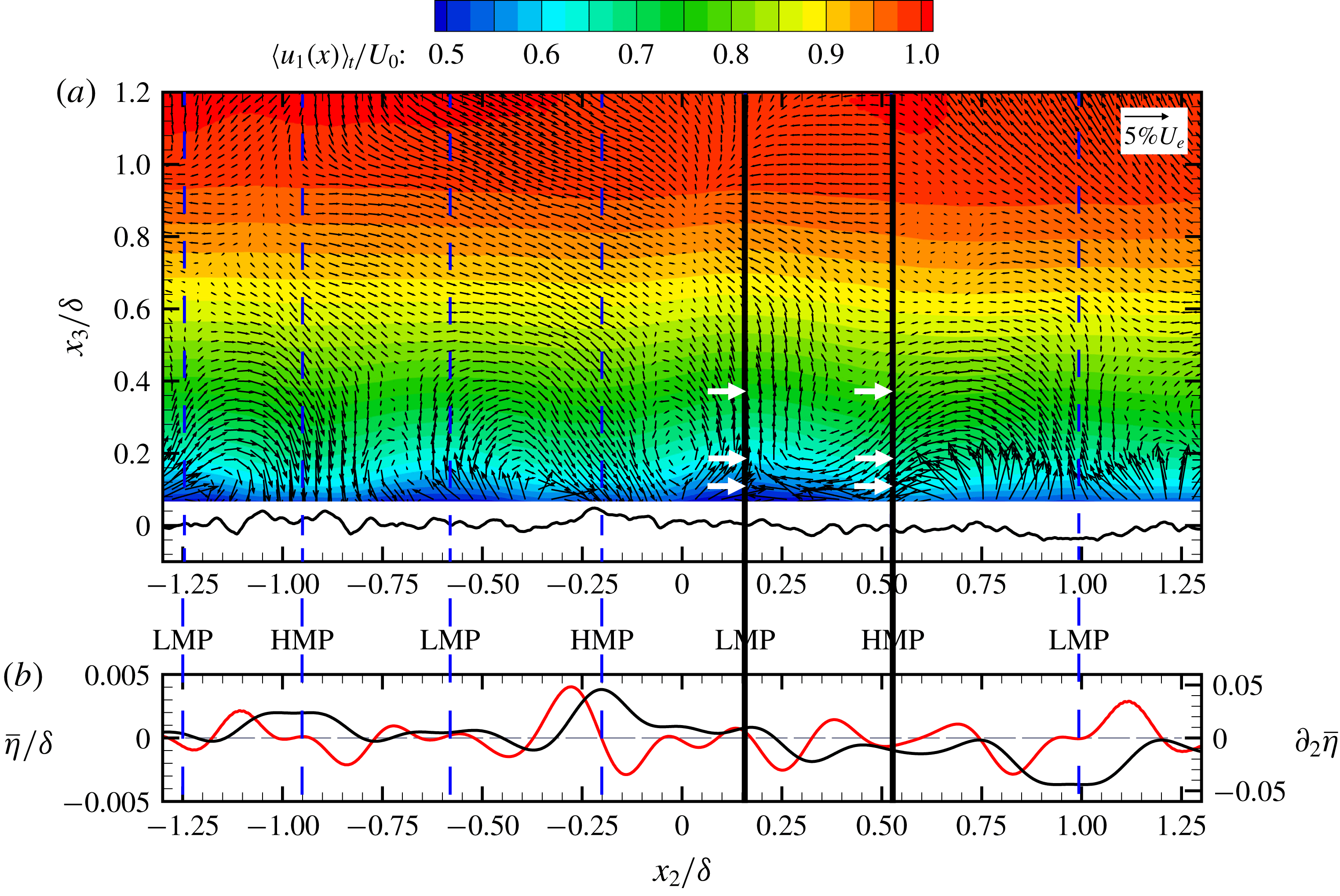
Mejia-Alvarez, Barros & Christensen (Reference Mejia-Alvarez, Barros, Christensen, Venditti, Best, Church and Hardy2013), Mejia-Alvarez & Christensen (Reference Mejia-Alvarez and Christensen2013) and Barros & Christensen (Reference Barros and Christensen2014) have shown how a complex roughness with predominant spanwise heterogeneity can alter the outer-layer dynamics (also shown in figure 8). They have shown how, in the spanwise–wall-normal plane, mean streamwise velocity exhibits spatial undulations over the depth of the flow,
 $\unicode[STIX]{x1D6FF}$
, and that mean streamwise momentum deficits are flanked by counter-rotating vortices with rotational sign such that there is positive wall-normal velocity (likewise, momentum excesses are flanked by counter-rotating vortices aligned such that there is negative vertical velocity). Mejia-Alvarez & Christensen (Reference Mejia-Alvarez and Christensen2010) refer to these deficits and excesses in mean streamwise momentum as low- and high-momentum pathways (LMP, HMP), respectively, a nomenclature that draws distinction against low- and high-momentum regions (LMR, HMR), coherent structures with an inherent transience (Ganapathisubramani et al.
Reference Ganapathisubramani, Longmire and Marusic2003; Hutchins & Marusic Reference Hutchins and Marusic2007a
).
In related work, Nugroho, Hutchins & Monty (Reference Nugroho, Hutchins and Monty2013) have studied turbulent boundary layer flows over spanwise-heterogeneous roughness constructed from herringbone roughness, and reported phenomena similar to Mejia-Alvarez et al. (Reference Mejia-Alvarez, Barros, Christensen, Venditti, Best, Church and Hardy2013), Mejia-Alvarez & Christensen (Reference Mejia-Alvarez and Christensen2013), Barros & Christensen (Reference Barros and Christensen2014). Nugroho et al. (Reference Nugroho, Hutchins and Monty2013) also reported spanwise thickening and thinning of the boundary layer depth (i.e.
 $\unicode[STIX]{x1D6FF}(x_{1})\rightarrow \unicode[STIX]{x1D6FF}(x_{1},x_{2})$
), and they showed that locations of maxima and minima in
 $\unicode[STIX]{x1D6FF}(x_{1},x_{2})$
correspond to spanwise roughness transitions. In subsequent work from this group, the locations of downwelling and upwelling were clearly associated with the spanwise locations of surface characteristic change (Kevin et al.
Reference Monty, Bai, Pathikonda, Nugroho, Barros, Christensen and Hutchins2017; Kevin, Monty & Hutchins Reference Monty and Hutchins2019). In open-channel flows relevant to river hydraulics, wherein the lower surface was composed of spanwise-adjacent ‘panels’ of high and low roughness, there have been sustained efforts to characterize observations of mean flow heterogeneity as a turbulent secondary flow phenomenon (Bradshaw Reference Bradshaw1987; Nezu & Nakagawa Reference Nezu and Nakagawa1993; Wang & Cheng Reference Wang and Cheng2005; Vermaas, Uijttewall & Hoitink Reference Vermaas, Uijttewall and Hoitink2011).
Willingham et al. (Reference Willingham, Anderson, Christensen and Barros2013) used LES to model turbulent channel flow over spanwise-adjacent ‘stripes’ of high and low roughness, and compared these against the earlier measurements from Mejia-Alvarez et al. (Reference Mejia-Alvarez, Barros, Christensen, Venditti, Best, Church and Hardy2013). The resulting mean flows exhibited strong qualitative agreement: positive and negative vertical velocity – upwelling and downwelling, respectively – occurs above relatively low and high roughness, respectively. In a later study, Anderson et al. (Reference Anderson, Barros, Christensen and Awasthi2015) used the transport equations for Reynolds-averaged turbulent kinetic energy and mean streamwise vorticity to comprehensively demonstrate that the turbulent secondary flows were Prandtl’s secondary flow of the second kind (Prandtl Reference Prandtl1952; Brundrett & Baines Reference Brundrett and Baines1964; Perkins Reference Perkins1970; Gessner Reference Gessner1973; Bradshaw Reference Bradshaw1987). That is, spatial heterogeneity of components of the Reynolds stress tensor in the spanwise–wall-normal plane is responsible for sustenance of the mean secondary flows. We also note contributions from Jelly, Jung & Zaki (Reference Jelly, Jung and Zaki2014) and Lee, Jelly & Zaki (Reference Lee, Jelly and Zaki2015), who considered spanwise heterogeneous surface texturing attained by variation of hydrophobicity. They also observed turbulent secondary flows and comprehensively demonstrated that these flows were Prandtl’s secondary flow of the second kind. In another recent article, Chung, Monty & Hutchins (Reference Chung, Monty and Hutchins2018) used DNS to study the resultant flow patterns due to spanwise changes in roughness, and found conceptually similar results to those reported in similar LES studies (Willingham et al. Reference Willingham, Anderson, Christensen and Barros2013).
Given the preponderance of evidence demonstrating that spanwise spacing,
 $s_{2}/\unicode[STIX]{x1D6FF}$
, is, indeed, a relevant roughness parameter, Yang & Anderson (Reference Yang and Anderson2017) performed a parametric study to precisely quantify how the flow – spatial attributes and intensity of secondary circulations – changes with spacing. Using canonical spanwise-heterogeneous cases resembling those shown in figure 1 – i.e. those composed of just one or a few characteristic scales – they demonstrated that the flow state falls within one of three regimes, depending on spacing:
(a) roughness regime:
 $s_{2}/\unicode[STIX]{x1D6FF}\lesssim 1$
, within which secondary circulations occupy regions in the immediate vicinity of the elements and continue to grow in spatial extent with increasing spacing;
(b) transitional regime:
$1\lesssim s_{2}/\unicode[STIX]{x1D6FF}\lesssim 3$
; and(c) topography regime:
$s_{2}/\unicode[STIX]{x1D6FF}\gtrsim 3$
, within which secondary circulations remain in the immediate vicinity of the elements, but their spatial extent is limited by the depth of the flow.


The studies cited herein for wall turbulence have consistently found that the cells are organized such that downwelling of high-momentum fluid is directed towards the ‘more rough’ regions of the surface. However, results from others have found a precise opposite. Ganapathisubramani and company have used numerical simulations and experiments to study turbulent boundary flow over a surface with spanwise heterogeneity derived from LEGO elements (Vanderwel & Ganapathisubramani Reference Vanderwel and Ganapathisubramani2015; Medjnoun, Vanderwel & Ganapathisubramani Reference Medjnoun, Vanderwel and Ganapathisubramani2018; Vanderwel et al. Reference Vanderwel, Stroh, Kriegseis, Frohnapfel and Ganapathisubramani2019). Their results are consistent with earlier results from complementary studies (Goldstein & Tuan Reference Goldstein and Tuan1998). Isolation of the processes responsible for setting the direction sign is not the target of this article. Moreover, we contend that the focus of this article transcends contemporary challenges associated with predicting directional sign.
In related experimental measurements of flow over the figure 8 roughness, Pathikonda & Christensen (Reference Pathikonda and Christensen2017) used hot-wires to record very long time-series measurements within high- and low-momentum pathways to assess how such Reynolds-averaged flow features affect inner–outer interactions (IOI). They also used particle image velocimetry (PIV) measurements to illustrate the spatial nature of IOI. With these datasets, they could quantify the nature of amplitude and frequency modulation (AM, FM) within HMPs and LMPs (Mathis, Hutchins & Marusic Reference Mathis, Hutchins and Marusic2009; Marusic, Mathis & Hutchins Reference Marusic, Mathis and Hutchins2010; Mathis, Hutchins & Marusic Reference Mathis, Hutchins and Marusic2011; Mathis et al.
Reference Mathis, Marusic, Chernyshenko and Hutchins2013; Baars et al.
Reference Baars, Talluru, Hutchins and Marusic2015). Awasthi & Anderson (Reference Awasthi and Anderson2018) used LES to study flow over a surface composed of large-scale geometric elements (
 $\unicode[STIX]{x1D6FF}/h\approx 8$
) with spanwise spacing of
 $\unicode[STIX]{x03C0}\unicode[STIX]{x1D6FF}$
between the peaks of elements; in this approach, HMPs and LMPs were guaranteed to form above the relative peak and trough of the roughness elements, respectively. By setting the location of HMPs and LMPs a priori, Awasthi & Anderson (Reference Awasthi and Anderson2018) were able to quantify AM and FM in a canonical arrangement. The work showed that with HMPs and LMPs, the spectral ‘outer peak’ is attenuated and preserved, respectively.
1.2 This article
In this article, results from LES and experimental measurement have been used to study unsteadiness in the turbulent secondary flows. All preceding studies have confirmed that spanwise-heterogeneous surface conditions induce Reynolds-averaged secondary flows – some have found downwelling of high-momentum fluid above the relatively ‘more rough’ regions, others have found the opposite – but time variation of the secondary cell intensity (and sign) has not been considered. We will show results from a suite of LES cases in which spacing and the height of elements is varied, in such a way that the three spacing regimes are targeted (roughness, transitional and topography). Using instantaneous, conditionally and Reynolds-averaged flow visualization, we will show that downwelling or upwelling can occur above the crest. The conditional sampling thresholds are selected based on probability density functions (p.d.f.) of velocity time series, which confirm non-trivial probability of system reversals occurrence. In addition, and in order to diversify the study, we also show results from experimental measurement of turbulent boundary layer flow over the figure 8 complex roughness profile. We show time series and p.d.f.s, where the former shows clear reversals from the established downwelling or upwelling patterns while the latter confirms the probability of large-scale reversals. There is precedent for these results based on Kevin et al. (Reference Monty, Bai, Pathikonda, Nugroho, Barros, Christensen and Hutchins2017), who decomposed the Reynolds-averaged secondary flow structure recovered from turbulent boundary layer flow over a herringbone roughness pattern. They, indeed, observed that the Reynolds-averaged pattern is rarely evident in the decomposed flow, and instead more complex patterns are observed.
Having established via LES and experiments that large-scale system reversals are possible, we have sought to study the system in more depth. Via projection of the base flow for streamwise velocity and streamwise vorticity upon a severely truncated Galerkin projection, and predicated upon a vortex forcing model for the dynamical influence of surface-driven rotation, we have studied underlying dynamics of the system (Waleffe Reference Waleffe1998). The vortex forcing is derived from long-term efforts to model Langmuir turbulence in the ocean mixed layer (Stokes Reference Stokes1847; Leibovich Reference Leibovich1977, Reference Leibovich1980, Reference Leibovich1983; Craik Reference Craik1985; McWilliams, Sullivan & Moeng Reference McWilliams, Sullivan and Moeng1997; Yang et al. Reference Yang, Chen, Chamecki and Meneveau2015), and efficacy of this approach within LES was recently demonstrated by Anderson et al. (Reference Anderson, Yang, Shrestha and Awasthi2018).
We emphasize that the results presented herein are general, and not specific to flow over spanwise heterogeneities due to arrays of obstacles or changing surface roughness. Indeed, the present LES results consider an array of element spacing and height (
 $5\leqslant \unicode[STIX]{x1D6FF}/h\leqslant 20$
), where the smallest element height and spacing are approaching rough-wall conditions expected to exhibit outer-layer similarity (Flack et al.
Reference Flack, Schultz and Connelly2007). The experimental measurements are from turbulent boundary layer flow known to exhibit outer-layer similarity (Wu & Christensen Reference Wu and Christensen2010). Nevertheless, for this wide range of dynamical conditions (and different approaches), we will still show evidence of large-scale reversals.
The base flow projection is substituted within the governing transport equations for streamwise velocity and streamwise vorticity; following a series of modest algebraic developments, a system closely resembling the Lorenz system is attained (Saltzman Reference Saltzman1962; Lorenz Reference Lorenz1963). The Lorenz system predicts the dynamical evolution of large-scale roll modes where the driving parameters are the Richardson and Reynolds numbers; in our system, the vortex forcing magnitude plays a role analogous to the Richardson number. With this, it is shown that under certain conditions, chaotic (non-periodic) phase-space orbits are possible, which represent the system reversals observed in the accompanying LES and experimental cases. The reversals occur as the system orbit approaches a saddle point, which is detailed in the following results. A series of developments are made to further study the system, which concludes with Poincaré projection to determine the attractor fractal dimension via correlation fractal dimension. The base flow projections and resultant system are predicated upon a series of assumptions and conditions, which are clearly emphasized throughout the development. Its simplicity notwithstanding, the propensity for chaotic, non-periodic trajectories in the base flow model suggests similar dynamics is responsible for the large-scale reversals observed in the LES and experimental datasets.
The results from complementary LES and experimental measurement are shown in § 2. In §§ 3 and 4, the governing equations, system derivation and numerical integration procedure are presented. Having derived the full system, results of scaling analysis of the Reynolds-averaged system are shown in § 5, while implications of the base flow projection for the spatial distribution of turbulent kinetic energy are presented in § 6. Finally, § 7 presents the aforementioned Poincaré projection and computation of system fractal dimension via correlation dimension. Concluding remarks are presented in § 8. For brevity within the text, three additional appendices are included to summarize the LES code (appendix A), the experimental measurement procedure and facility (appendix B) and the first- to fourth-order partial derivatives of the truncated Galerkin projection base flow models (appendix C).
It must be noted that the present article adds to an existing body of literature on the chaotic nature of shear flows. Foremost among preceding activity is the seminal work of Lorenz (Reference Lorenz1963), who revealed the chaotic nature of a base flow representing unsteady roll cells in an unstably stratified, buoyancy-driven wall flow. Others, however, have also explored the underlying dynamics of shear flows at a range of scales. For example, the nature of two-dimensional vortices resembling those observed in geophysical flows has been studied at length by Bouchet and company (Bouchet & Barré Reference Bouchet and Barré2005; Bouchet & Simonnet Reference Bouchet and Simonnet2009; Bouchet & Venaille Reference Bouchet and Venaille2012; Laurie & Bouchet Reference Laurie and Bouchet2015). These articles have demonstrated the tendency for sudden, large-scale reversals. More recently, Brunton, Proctor & Kutz (Reference Brunton, Proctor and Kutz2016) demonstrated that projection of the leading mode from proper orthogonal decomposition of canonical shear flows can be cast as a dynamical system, which enables assessment of the periodic or non-periodic orbit of the peak energy-containing modes (Holmes, Lumley & Berkooz Reference Holmes, Lumley and Berkooz1996).
There are some conceptual similarities between the present work and the contributions from McKeon and company, who presented models for the elongated structures present in turbulent Couette flow (see, for example, Gayme et al. Reference Gayme, McKeon, Papachristodoulou, Bamieh and Doyle2010). However, the present work is distinctly different as the results are directed towards streamwise-homogeneous secondary rolls, and not the topology of structures emergent from the frameworks developed by McKeon and company. For completeness, we also point out that for transitional boundary layers, Townsend (Reference Townsend1976) developed a prognostic tool for the onset of persistent rolls originating from lateral stress variations (de Silva et al. Reference de Silva, Baidya, Hutchins and Marusic2018). This prognostic tool was derived from the Reynolds-averaged vorticity transport equation – the equation underpinning this work – but was used for an entirely different purpose (here, spanwise surface-stress variation is imposed via a proxy model for topographic heterogeneity, and we are concerned with inertial-dominated flows).
2 Results from simulations and experiments
In order to provide a context for results of the dynamical systems assessment noted in § 1.2, results from a wide-ranging LES study (§ 2.1) and experimental measurement campaign (§ 2.2) are presented here. The LES study is designed to reveal systematic variation in the flow state with changing surface attributes – element height and spacing between adjacent rows,
 $s_{2}/\unicode[STIX]{x1D6FF}$
– and these canonical arrangements provide a means to clearly quantify changing flow state and intensity. In contrast, the experimental data are from turbulent boundary layer flow over a complex roughness (Bons et al.
Reference Bons, Taylor, McClain and Rivir2001), which exhibits significant streamwise elongation relative to the spanwise properties (see, for example, Mejia-Alvarez & Christensen Reference Mejia-Alvarez and Christensen2010, for evidence of this). Using conditional sampling based on probability density functions of vertical velocity within a HMP, we are able to demonstrate that both upwelling and downwelling is possible above the crest of roughness elements.
2.1 Large-eddy simulation
The LES code has been used for many years to model high-
 $Re_{\unicode[STIX]{x1D70F}}$
turbulent channel flow (resembling conditions within planetary atmospheric boundary layers, although for the present application we consider high Rossby number and neutral thermal stratification, i.e. turbulence is sustained exclusively by mechanical shear). Appendix A contains a comprehensive description of the LES code, and specific details of the computational mesh for the simulations performed for this study. Thus, we refer the interested reader to appendix A for further clarification on the LES code. Note that quantities resolved during LES are denoted by tilde, i.e.
 $\tilde{\boldsymbol{u}}=G_{\unicode[STIX]{x1D6E5}}\star \boldsymbol{u}$
, where
 $G_{\unicode[STIX]{x1D6E5}}$
is a filtering kernel at grid-filter scale,
 $\unicode[STIX]{x1D6E5}$
, and
 $\star$
denotes the convolution operator. As per (A 3) and accompanying text, the total (Reynolds) stress tensor,
 $\unicode[STIX]{x1D64F}$
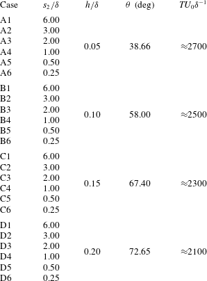
, is attained via the addition of its constituent resolved and subgrid-scale components. The LES code is used for 24 simulations, which enables parametric testing on the role of element height,
 $h$
, and spanwise spacing,
 $s_{2}/\unicode[STIX]{x1D6FF}$
, where the attributes of different cases are summarized in table 1 and figure 1.
Summary of LES case attributes.

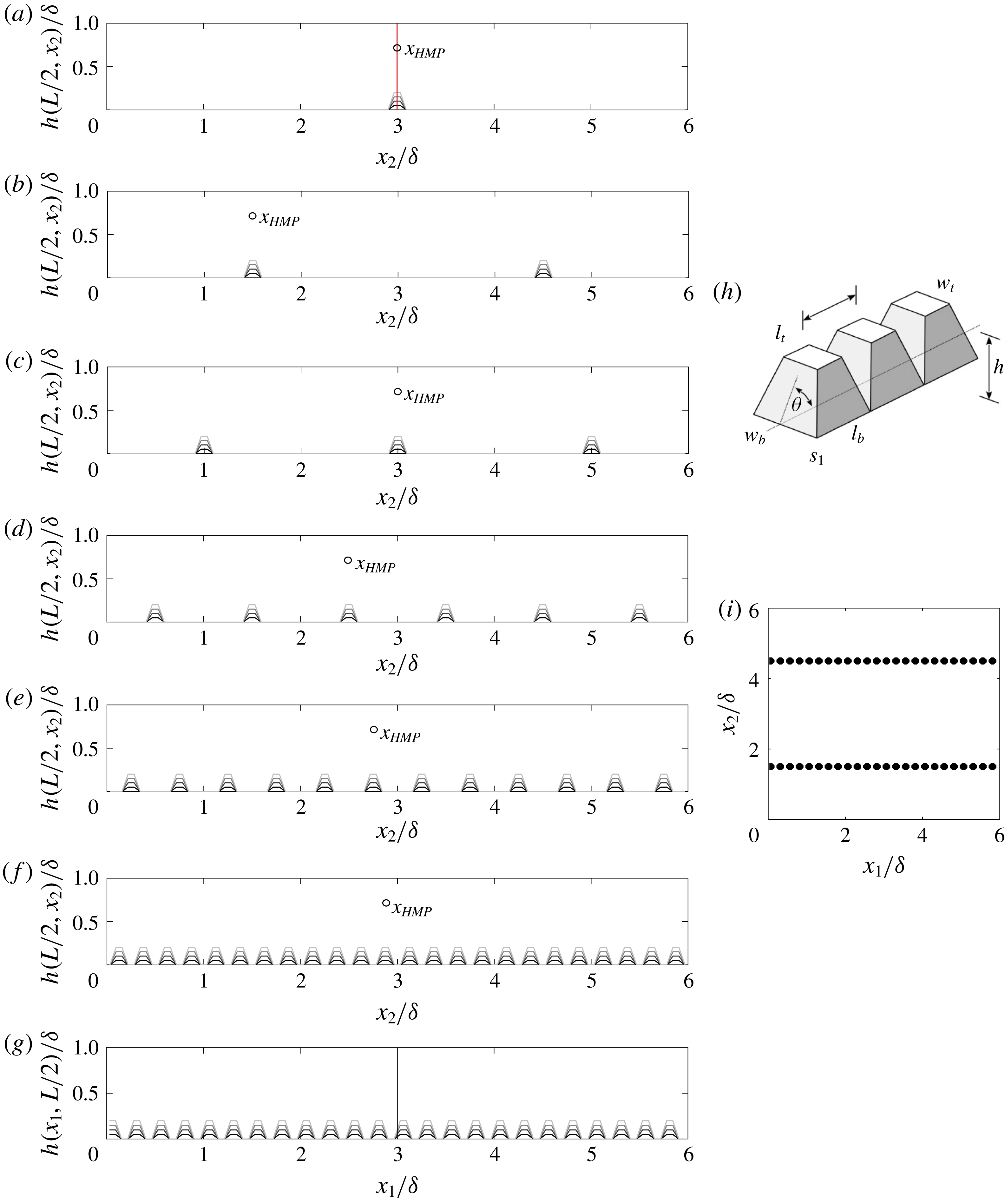
Figure 1 shows the geometric arrangements considered here, where the surfaces are composed of streamwise-aligned, vertically truncated, square-based pyramids, as highlighted in figure 1(h). The element heights,
 $h/\unicode[STIX]{x1D6FF}$
, are summarized in table 1, where the values vary in the range
 $5\leqslant \unicode[STIX]{x1D6FF}/h\leqslant 20$
; these values indicate outer-layer similarity may only be exhibited by Cases A5 and A6 (i.e. those most closely resembling a roughness; see table 1 for details) (Flack et al.
Reference Flack, Schultz and Connelly2007). Beyond the element ‘steepness’, denoted by
 $\unicode[STIX]{x1D703}$
in table 1 and figure 1(h), all other element attributes are summarized in § A.1 (i.e.
 $w_{b}$
,
 $l_{b}$
,
 $l_{t}$
,
 $w_{t}$
and
 $s_{1}$
). As per appendix A, results of computational mesh resolution sensitivity have not been included in this study. This topic has been thoroughly addressed in recent studies, for example Yang & Anderson (Reference Yang and Anderson2017) or, more recently, Awasthi & Anderson (Reference Awasthi and Anderson2018).
In fact, Yang & Anderson (Reference Yang and Anderson2017) used LES to model flow over geometric arrangements similar to those studied for this work, and the flow statistics (including the spatial attributes and coherence of turbulence above the element crests and troughs) exhibited no discernible response to changing computational mesh resolution. Moreover, the intensity and spatial nature of topography-induced, Reynolds-averaged turbulent secondary flows were shown to be insensitive to resolution (at least, over the range of resolutions considered in Yang & Anderson Reference Yang and Anderson2017, which encompass the mesh resolution considered for the present article). Note, also, that Awasthi & Anderson (Reference Awasthi and Anderson2018) present results of LES of flow over surfaces that exhibit geometric resemblance to those considered here – at least, in the sense that they considered large-scale elements with large spanwise spacing – and they presented statistics including spectrograms and correlation profiles between small- and large-scale content via modulation of small-scale frequency and amplitude. Resolution sensitivity was of foremost importance in Awasthi & Anderson (Reference Awasthi and Anderson2018), yet their results exhibited virtually no response to changing resolution. For these reasons, and in the interest of brevity, we consider the role of resolution to have been sufficiently addressed in preceding studies, and we have thus not included such results as part of this article.
Visualization of LES cases. (a–f) Show visualization in the spanwise–wall-normal plane, while (g) shows visualization in the streamwise–wall-normal plane. (h) Shows perspective visualization of the roughness elements with annotations for geometric attributes, while (i) shows a planform visualization of Case A2, for perspective. In (a–g), line colours correspond to cases A
 $i$
(black), B
 $i$
(dark grey), C
 $i$
(grey) and D
 $i$
(light grey), where
 $i=1$
, 2, 3, 4, 5 and 6 (see table 1 for summary of case attributes). (a–f) Show cases with spacing,
 $s_{2}/\unicode[STIX]{x1D6FF}=6$
, 3, 2, 1, 0.5 and 0.25, respectively. Vertical red line in (a) denotes the location at which the (g) streamwise–wall-normal transect is shown; vertical blue line in (g) denotes the location at which the (a) spanwise–wall-normal transect is shown. In (a–f), the discrete location,
 $\boldsymbol{x}_{HMP}$
, denotes the location at which time-series data were recorded.
 $\boldsymbol{x}_{HMP}$
was selected to be precisely above the crest of the row of elements.

Figure 1(a–f) presents visualization of topographic transects in the spanwise–wall-normal plane, where the cases are denoted by different colours, as per the figure caption. As is apparent from the figures, this selection of surfaces provides a means to measure the influence of changing surface element height,
 $h/\unicode[STIX]{x1D6FF}$
, and spanwise spacing,
 $s_{2}/\unicode[STIX]{x1D6FF}$
, where both values are summarized in table 1. Figure 1(a–f) provides visual context for the surfaces. As outlined in appendix A, the LES code uses spectral discretization in the horizontal direction, thus rendering the horizontal boundary conditions periodic. The perception of a lateral domain termination is incorrect, and instead one can envision infinite repetition of the domain in the spanwise and streamwise direction. For this reason, the spanwise spacing for Cases A1, B1, C1 and D1, for example, is
 $s_{2}/\unicode[STIX]{x1D6FF}=6$
, since periodic boundary conditions impose that the nearest adjacent rows are located at
 $x_{2}/\unicode[STIX]{x1D6FF}=-3$
and
 $x_{2}/\unicode[STIX]{x1D6FF}=9$
.
Note that Cases A1, B1, C1 and D1 are designed to capture a limiting spacing,
 $s_{2}/\unicode[STIX]{x1D6FF}=6$
, at which turbulent secondary flows are able to occupy the depth of the flow without any interference from adjacent cells (Anderson et al.
Reference Anderson, Barros, Christensen and Awasthi2015; Yang & Anderson Reference Yang and Anderson2017). Surfaces in this regime have previously been described as a topography, owing to the global response they impart in the above flow. In contrast, cases with the smallest spacing (A5, A6, B5, B6, C5, C6, D5 and D6; see also figure 1
e,f and table 1) are designed to behave as a roughness, in the sense that any element-induced Reynolds-averaged turbulent secondary flows will be located in the immediate vicinity of the elements, but with spatial extent constrained by the lateral spacing between adjacent rows. Turbulence statistics in the inertial layer, or outer layer, for these cases should exhibit no Reynolds-averaged heterogeneity (beyond those associated with the wall-normal mechanical shear production). For these cases, then, the Reynolds-averaged secondary cells are best understood as those typical of the roughness sublayer – the region of the flow occupied by element-scale vortices (Goldstein & Tuan Reference Goldstein and Tuan1998; Vanderwel & Ganapathisubramani Reference Vanderwel and Ganapathisubramani2015; Medjnoun et al.
Reference Medjnoun, Vanderwel and Ganapathisubramani2018).
It has been systematically shown that secondary cells within the roughness regime remain attached to the elements such that upwelling of low-momentum fluid occurs above the individual rows of elements (Vanderwel & Ganapathisubramani Reference Vanderwel and Ganapathisubramani2015; Yang & Anderson Reference Yang and Anderson2017; Medjnoun et al.
Reference Medjnoun, Vanderwel and Ganapathisubramani2018; Vanderwel et al.
Reference Vanderwel, Stroh, Kriegseis, Frohnapfel and Ganapathisubramani2019). In contrast, secondary cells within the topography regime are located in the outer layer such that downwelling of high-momentum fluid occurs above the rows of elements. When downwelling is directed towards relatively more rough regions of the surface, it is consistent with prior interpretation of high- and low-momentum pathways (Willingham et al.
Reference Willingham, Anderson, Christensen and Barros2013; Barros & Christensen Reference Barros and Christensen2014; Anderson et al.
Reference Anderson, Barros, Christensen and Awasthi2015), although we acknowledge that others have found opposite direction sign in complementary research. For this reason, we have added the discrete spatial marker,
 $\boldsymbol{x}_{HMP}$
, to figure 1(a–f), fully cognizant of the fact that in the roughness regime, the marker may not correspond to a HMP. Nevertheless, for Cases A1, B1, C1 and D1,
 $\boldsymbol{x}_{HMP}$
indeed corresponds to the location of a HMP, while for the transitional regime cases, we will demonstrate the probability for both to occur.
The selection of asymptotic roughness and topography regime cases ensures that the ensuing parameter variation is guaranteed to encompass the transitional regime, where both element-scale cells and HMP/LMP-type cells are possible (in §§ 3 and 4, we will demonstrate that a truncated Galerkin projection of transitional regime cells yields a system of ordinary differential equations, with orbits that undergo chaotic reversals about a phase-space saddle node). Results from LES of flow over the transitional cases selected for this study – Cases A2–A4, B2–B4, C2–C4 and D2–D4 – provide strong support for chaos as an underlying justification for the ostensible reversal in rotational sign from roughness to topography. The experimental results further this argument (§ 2.2). But, in both cases, the natural complexity of the problem and the presence of broadband mixing confounds efforts to isolate such chaotic mechanisms with clarity.
In figure 1(a), the vertical red line denotes the spanwise location at which the streamwise–wall-normal transect is shown in figure 1(g); likewise, the vertical blue line on figure 1(g) denotes the streamwise location at which the figure 1(a) transect is shown. Figure 1(h) provides further graphical context and perspective on the nature of the roughness elements; figure 1(i) shows a planform visualization of Case A2, for visual perspective.
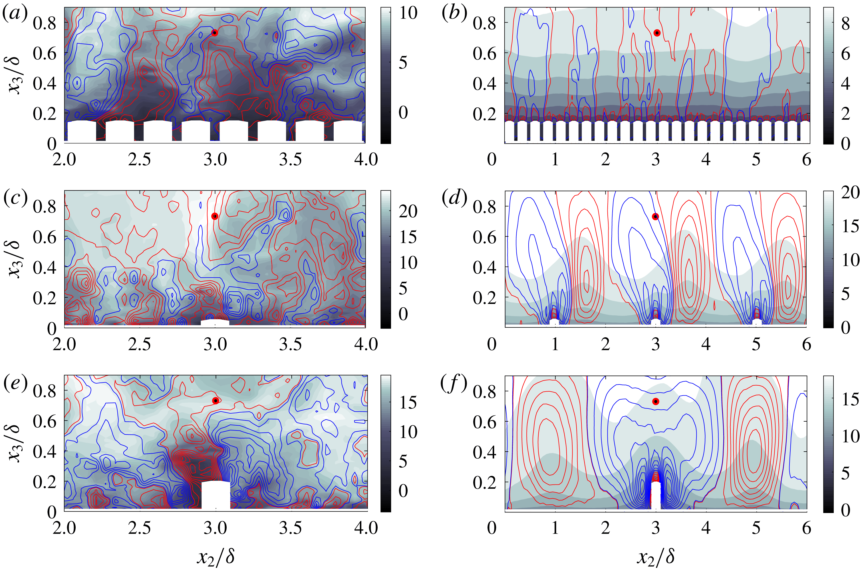
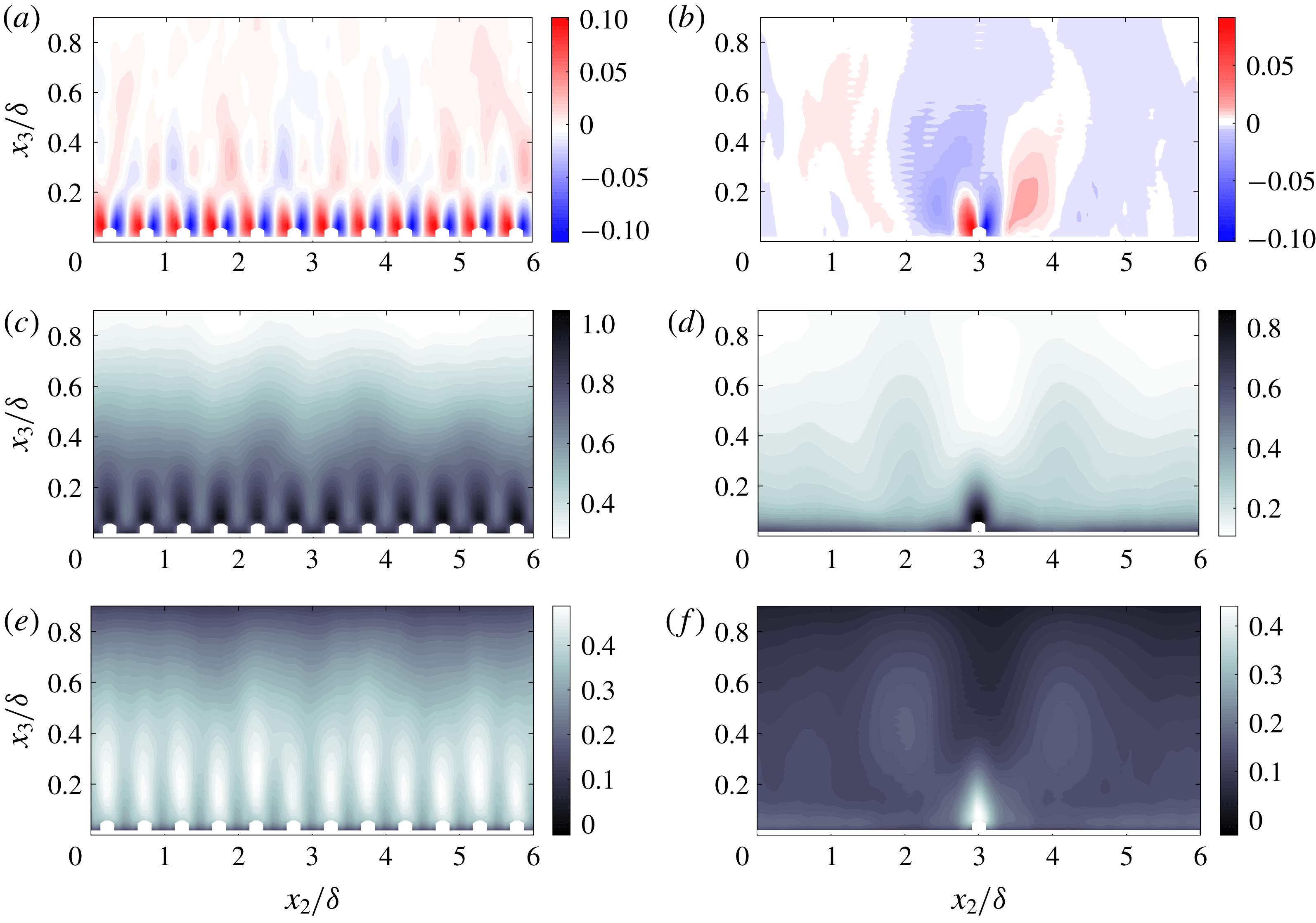
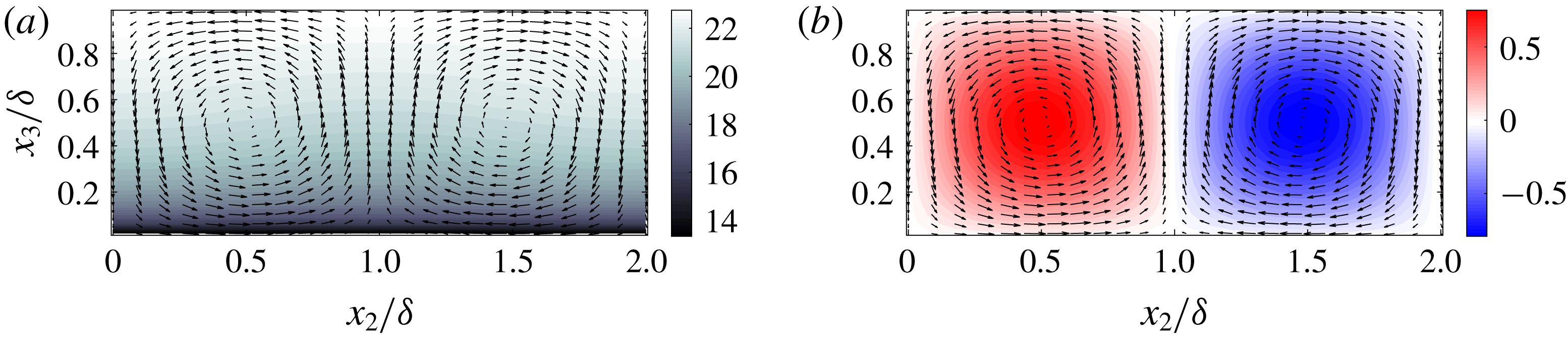
Instantaneous (a,c,e) and Reynolds-averaged (b,d,f) flow structure in the spanwise–wall-normal plane. Colour flood contour corresponds to streamwise velocity,
 $\tilde{u} _{1}/u_{\unicode[STIX]{x1D70F}}$
, while line contours represent positive (red) and negative (blue) components of vertical velocity,
 $\tilde{u} _{3}/u_{\unicode[STIX]{x1D70F}}$
. (a,b) Case C6; (c,d) Case A3; (e,f) Case D1. In all panels, location of discrete sampling point used for conditional averaging denoted by red circle with black fill. In a subsequent result, probability density functions of velocity at
 $\boldsymbol{x}_{HMP}$
will be used to demonstrate that
 $-2\lesssim \tilde{u} _{3}^{\prime }(\boldsymbol{x}_{HMP},t)\lesssim 4$
(see figure 6 and accompanying text), while figure 3 shows a wall-normal profile for Reynolds-averaged wall-normal velocity for Case D1 (f of the present figure). Note that (a,c,e) are shown over region,
 $2\leqslant x_{2}/\unicode[STIX]{x1D6FF}\leqslant 4$
, for clarity.

Figure 2 shows instantaneous (panels a,c,e) and Reynolds-averaged (panels b,d,f) contours of streamwise and wall-normal velocity in the spanwise–wall-normal plane. The specific cases are noted in the figure caption. The vertical velocity topographic contours were prepared such that regions of upwelling (positive wall-normal velocity; red) and downwelling (negative wall-normal velocity; blue) are emphasized. This approach aids interpretation of the streamwise velocity contours, since downwelling and upwelling are associated with streamwise momentum excesses and deficits, respectively. As per the caption, figure 3(b) shows wall-normal profiles of Reynolds-averaged vertical velocity for Case D1 (figure 2
f), while figure 6 shows p.d.f.s at
 $\boldsymbol{x}_{HMP}$
for a range of cases, which provide additional information on the mean and variability of
 $\tilde{u} _{3}^{\prime }(\boldsymbol{x},t)$
. For now, we note that the limiting negative and positive values of vertical velocity are
 $\tilde{u} _{3}^{\prime }(\boldsymbol{x},t)\approx -4$
and
 $\tilde{u} _{3}^{\prime }(\boldsymbol{x},t)\approx 4$
, respectively.
Beginning with the topography cases (figure 2
e,f), the instantaneous visualization shows a large plume of relatively low-momentum fluid immediately above the element, while the Reynolds-averaged contour clearly reveals a large (
 $\unicode[STIX]{x1D6FF}$
-scale) zone of streamwise momentum excess above the element (figure 2
f,
 $2\lesssim x_{2}/\unicode[STIX]{x1D6FF}\lesssim 4$
), which is concurrent with a large area of downwelling. This flow pattern is a clear manifestation of a HMP – as has been documented in previous studies (Willingham et al.
Reference Willingham, Anderson, Christensen and Barros2013; Barros & Christensen Reference Barros and Christensen2014; Anderson et al.
Reference Anderson, Barros, Christensen and Awasthi2015); note, however, a small zone of upwelling at the top of the element, owing to the presence of element-scale vortices (i.e. those that prevail exclusively for roughness regime surfaces). The large downwelling region (and momentum excess) is flanked by two large-scale zones of upwelling, which are concurrent with streamwise momentum excesses; this result is entirely consistent with HMP/LMP formation observed in prior studies.
Figure 2(a,b) shows instantaneous and Reynolds-averaged flow quantities for a roughness regime case. The instantaneous panel exhibits flow processes resembling those observed in flow over a homogeneous roughness, while the Reynolds-averaged panels show minimal inertial layer disturbances, with the exception of an undulation at
 $x_{2}/\unicode[STIX]{x1D6FF}\approx 4.8$
and
 $x_{3}/\unicode[STIX]{x1D6FF}\approx 0.8$
. This is a consequence of some modest transience within the flow that does not vanish with Reynolds averaging; for this study, every effort was made to attain truly Reynolds-averaged quantities. The number of large-eddy turnover times used to compute Reynolds averages is summarized in table 1 in the column with heading,
 $TU_{0}\unicode[STIX]{x1D6FF}^{-1}$
. We emphasize, also, that for all cases the averaging period was preceded by far longer development time. Nevertheless, such modest undulations are inherent to these simulations, as has been widely reported in prior studies (Reynolds et al.
Reference Reynolds, Hayden, Castro and Robins2007; Fishpool et al.
Reference Fishpool, Lardeau and Leschziner2009).
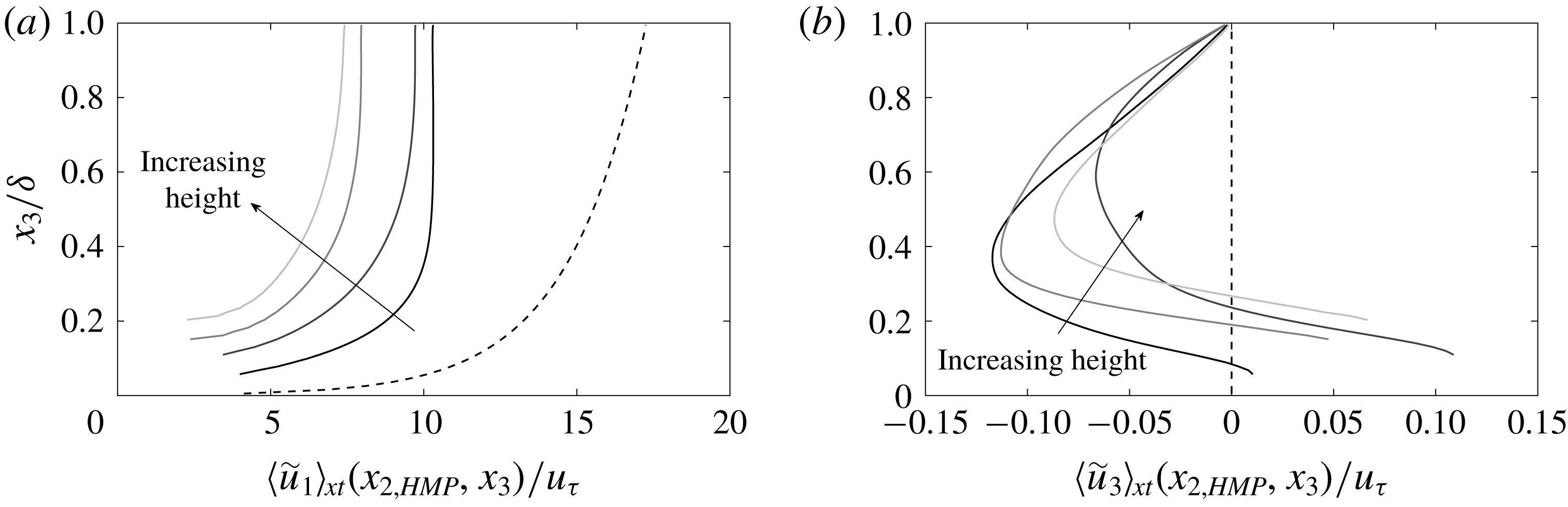
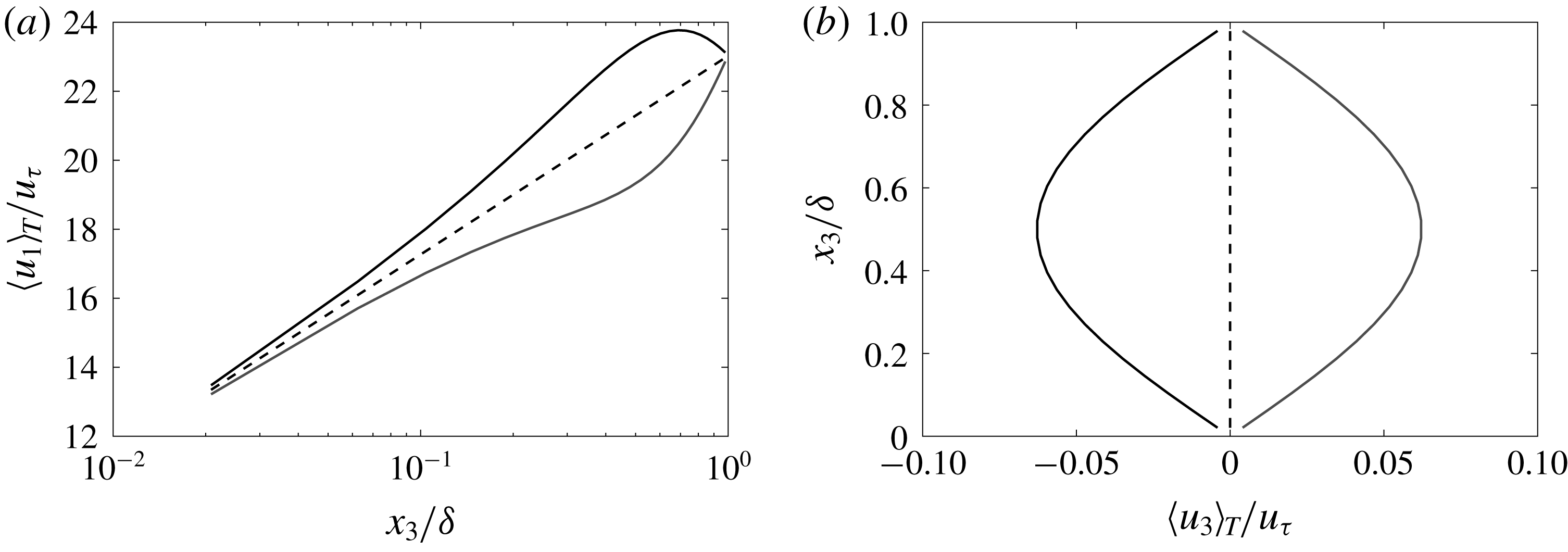
Vertical profiles of Reynolds-averaged streamwise (a) and vertical (b) velocity within a HMP (i.e. vertical transect coincident with
 $\boldsymbol{x}_{HMP}$
in figure 1
a). Profiles correspond to Case A1 (black), B1 (dark grey), C1 (grey) and D1 (light grey), where vertical shift to beginning of profiles is due to region occupied by solid topographic elements. For context, the canonical channel flow logarithmic streamwise velocity profile,
 $U_{1}(x_{3})/u_{\unicode[STIX]{x1D70F}}=\unicode[STIX]{x1D705}^{-1}\log (x_{3}/l)$
, and vertical velocity profile,
 $U_{3}(x_{3})/u_{\unicode[STIX]{x1D70F}}=0$
, are shown with a dashed black line on panels (a) and (b), respectively. Direction of increasing element height added for perspective.

Finally, figure 2(c,d) shows instantaneous and Reynolds-averaged flow patterns for a transitional case. The instantaneous visualization, again, shows large-scale mixing over the depth of the flow, while the Reynolds-averaged streamwise velocity colour flood shows large-scale heterogeneities that are driven by the spanwise surface heterogeneity. Although the structures exhibit a lateral inclination, the vertical velocity contours demonstrate that HMPs are collocated with the rows of elements – that is, regions of downwelling occupy the zone above the element, and this overlaps precisely with streamwise momentum excesses in the outer layer, which is evidence of a HMP. Likewise, regions of net upwelling are present and overlap regions of streamwise velocity deficit, which indicates manifestation of an LMP. This lateral inclination is commonly observed, and is thought to be associated with insufficient time averaging (although, long time-averaging periods were used, as per table 1), or with numerical attributes of the LES code (Willingham et al. Reference Willingham, Anderson, Christensen and Barros2013). The pattern does not exhibit the same level of organization as attained for the topography case (i.e. see figure 2 f), but the Reynolds-averaged visualization is consistent with prior results on the position of HMPs and LMPs. Conditional sampling will show, however, that large-scale reversals occur with high probability.
In order to highlight flow structure within a HMP, figure 3(a,b) shows Reynolds-averaged streamwise and wall-normal velocity profiles at a spanwise location intersecting the HMP sampling point in figure 1(a). The profiles are for Cases A1, B1, C1 and D1 – i.e. those for which a distinct HMP resides above the elements – and for context we have included profiles for a canonical channel flow (logarithmic profile in figure 3
a and zero wall-normal velocity in figure 3
b). The origin at which each profile begins is vertically displaced by virtue of the presence of the elements. The immersed boundary method used for the simulations sets the velocity at internal, ‘immersed’ grid points to zero (all details of the LES code and immersed boundary method are provided in appendix A). It is clear, firstly, that the streamwise profiles are not logarithmic – instead, they exhibit a wall-normal gradient ostensibly greater than that for a logarithmic profile,
 $u_{\unicode[STIX]{x1D70F}}(\unicode[STIX]{x1D705}x_{3})^{-1}$
.
Moreover, the profiles attain a zero-stress state far lower in the domain, for example at
 $x_{3}/\unicode[STIX]{x1D6FF}\approx 0.5$
for Case A1. This larger wall-normal gradient is entirely consistent with prior work by Anderson et al. (Reference Anderson, Barros, Christensen and Awasthi2015), who demonstrate that a production–dissipation imbalance in turbulent kinetic energy,
 $tke$
, above the relatively more rough regions (i.e. at spanwise locations corresponding to HMPs) was the underlying mechanism responsible for sustenance of the secondary flows (Hinze Reference Hinze1967; Bradshaw Reference Bradshaw1987). As would be expected, increasing the element height imposes a greater momentum penalty upon the flow, thereby reducing the centreline velocity: the figure demonstrates a monotonic reduction in outer velocity.
For all cases, figure 3(b) clearly demonstrates a region of downwelling over the depth of the flow (for Case D1, this is also apparent from inspection of figure 2f). However, when the profiles are presented in this format, an apparent reduction in the magnitude of
 $\langle \tilde{u} _{3}\rangle _{xt}(x_{2,HMP},x_{3})<0$
is apparent, while the magnitude of
 $\langle \tilde{u} _{3}\rangle _{xt}(x_{2,HMP},x_{3})>0$
in the near-wall region increases. This is a product of local, element-scale roughness sublayer mixing, and is also visible in figure 2(e,f). When these element-scale vortices are produced in close proximity to the surface, ambient background shear associated with the wall serves to homogenize their influence (i.e. Case A1 profiles in figure 3). However, when produced due to the presence of larger elements, the element-scale vortices are naturally larger, thereby inducing higher wall-normal velocities above the crest and weakening the subsequent downwelling.
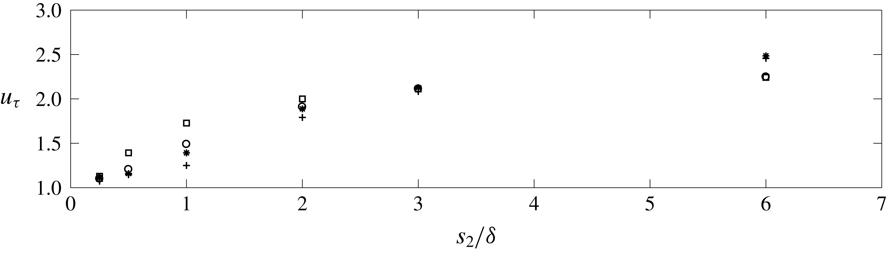
Data points for post-normalization shear velocity,
 $u_{\unicode[STIX]{x1D70F}}=(\text{max}|\unicode[STIX]{x1D61B}_{13}|)^{1/2}$
. Grey panel added to denote transitional regime. Symbols denote group of cases: ‘plus’ sign (Cases A1–A6), asterisk (Cases B1–B6), circle (Cases C1–C6) and square (Cases D1–D6).

For completeness, figure 4 shows the shear velocity attained via
 $u_{\unicode[STIX]{x1D70F}}=(\text{max}|\unicode[STIX]{x1D61B}_{13}|)^{1/2}$
. For flow over a homogeneous sandpaper distribution, the LES shear velocity is, by definition,
 $u_{\unicode[STIX]{x1D70F}}=1$
, and these values actually occur in the roughness regime (in an approximate sense). However, with increased spacing,
 $u_{\unicode[STIX]{x1D70F}}$
increases as large-scale flow heterogeneities emerge in the flow, and local peaks in
 $\unicode[STIX]{x1D61B}_{13}$
are concentrated above the elements (Awasthi & Anderson Reference Awasthi and Anderson2018). By post-normalizing the statistics with this
 $u_{\unicode[STIX]{x1D70F}}$
, the results can be properly compared. In a subsequent result, probability density functions from
 $\boldsymbol{x}_{HMP}$
are presented, but before doing so some additional results on the underlying driving mechanism are presented.
Anderson et al. (Reference Anderson, Barros, Christensen and Awasthi2015) showed that the turbulent secondary flows associated with HMPs and LMPs – i.e. for which a streamwise momentum excess and downwelling occurs above the relative peaks in surface roughness – are a manifestation of Prandtl’s secondary flow of the second kind (Bradshaw Reference Bradshaw1987). In doing so, Anderson et al. (Reference Anderson, Barros, Christensen and Awasthi2015) used the Reynolds-averaged transport equation for streamwise vorticity and
 $tke$
. In a later section of this article, the
 $tke$
transport equation is reviewed again; for this stage, however, the Reynolds-averaged streamwise vorticity transport equation is apropos:
 $$\begin{eqnarray}\langle \tilde{u} _{2}\rangle _{T}\unicode[STIX]{x2202}_{2}\langle \tilde{\unicode[STIX]{x1D714}}_{1}\rangle _{T}+\langle \tilde{u} _{3}\rangle _{T}\unicode[STIX]{x2202}_{3}\langle \tilde{\unicode[STIX]{x1D714}}_{1}\rangle _{T}=(\unicode[STIX]{x2202}_{3}^{2}-\unicode[STIX]{x2202}_{2}^{2})\langle \unicode[STIX]{x1D61B}_{23}\rangle _{T}+\unicode[STIX]{x2202}_{23}(\langle \unicode[STIX]{x1D61B}_{22}\rangle _{T}-\langle \unicode[STIX]{x1D61B}_{33}\rangle _{T}),\end{eqnarray}$$
where the tensor components,
 $\langle \unicode[STIX]{x1D61B}_{23}\rangle _{T}$
,
 $\langle \unicode[STIX]{x1D61B}_{22}\rangle _{T}$
and
 $\langle \unicode[STIX]{x1D61B}_{33}\rangle _{T}$
, are retrieved a posteriori from
 $\langle \unicode[STIX]{x1D64F}\rangle _{T}$
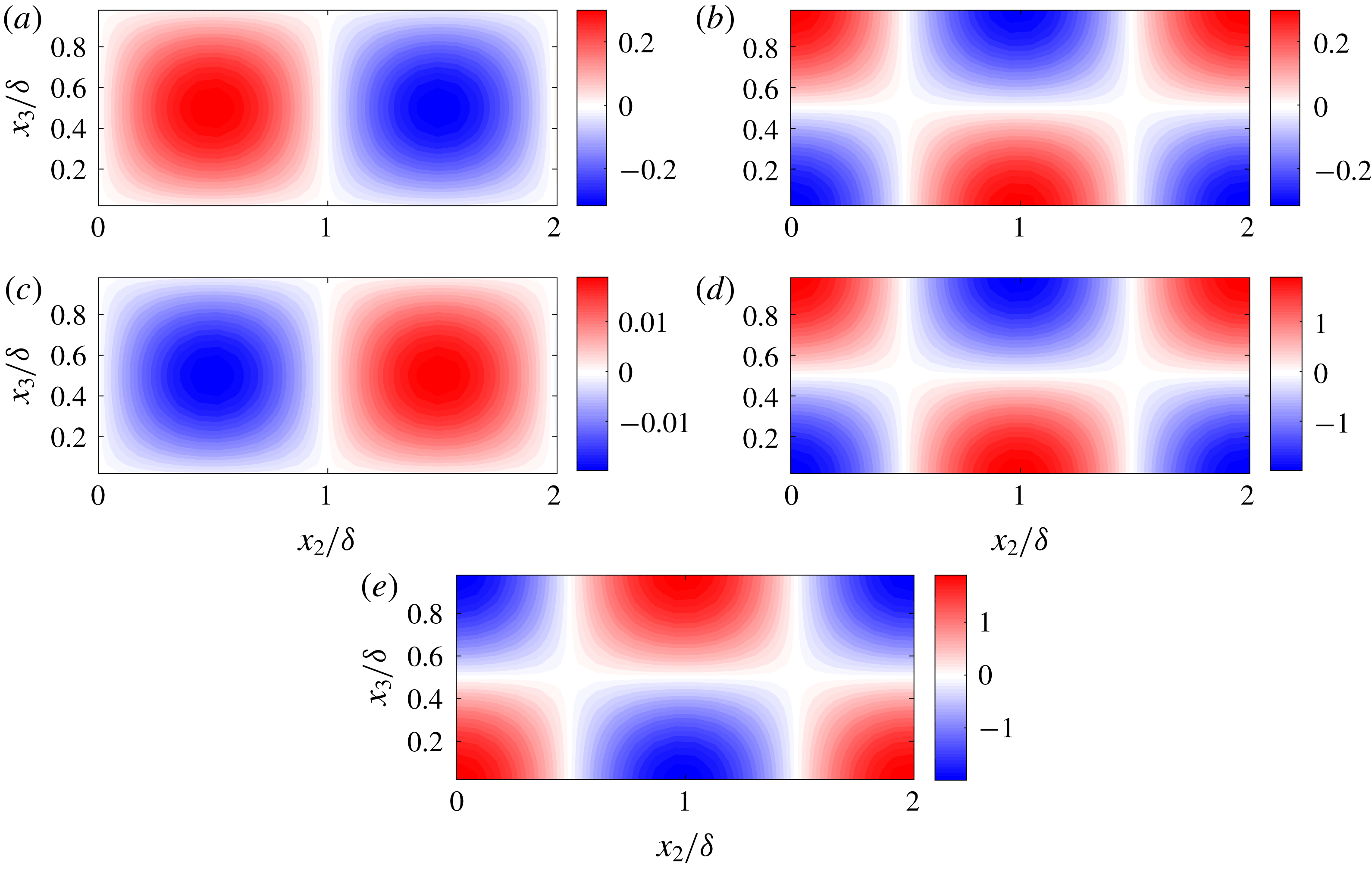
via the sum of contributions from the resolved and subgrid-scale components (see also (A 3) and accompanying text). Upon inspection of (2.1), it is immediately apparent that in the absence of Reynolds stress spatial heterogeneity, no secondary flow is possible. Figure 5 shows colour flood contours of Reynolds stress terms appearing in (2.1), where underlying spatial heterogeneity is responsible for the non-zero left-hand side terms.
Reynolds (turbulent) stresses responsible for Prandtl’s secondary flow of the second kind (see also (2.1) and accompanying text). (a,c,e) and (b,d,f) show results for Cases A5 (roughness regime) and A1 (topography regime), respectively. Colour flood contours correspond to
 $\unicode[STIX]{x1D61B}_{23}/u_{\unicode[STIX]{x1D70F}}^{2}$
(a,b),
 $\unicode[STIX]{x1D61B}_{22}/u_{\unicode[STIX]{x1D70F}}^{2}$
(c,d), and
 $\unicode[STIX]{x1D61B}_{33}/u_{\unicode[STIX]{x1D70F}}^{2}$
(e,f).

Contours are shown for cases in the roughness (figure 5
a,c,e) and topography (figure 5
b,d,f) regime, where case details are summarized in the figure caption. Since
 $\langle \tilde{\unicode[STIX]{x1D714}}_{1}\rangle _{T}\rightarrow 0$
in the absence of spatial heterogeneity of
 $\langle \unicode[STIX]{x1D61B}_{23}\rangle _{T}$
,
 $\langle \unicode[STIX]{x1D61B}_{22}\rangle _{T}$
, and
 $\langle \unicode[STIX]{x1D61B}_{33}\rangle _{T}$
, the emergence of a channel-like inertial layer in the roughness regime is understood from inspection of figure 5(a,c,e), where all components approach zero for
 $x_{3}/\unicode[STIX]{x1D6FF}\gtrsim 0.5$
. For the topography regime, regions of high-intensity turbulent stresses are still present in the immediate vicinity of the elements (note that figures 5
a,c,e and 5
b,d,f correspond to the same element height). In addition, however, are the zones of elevated stresses over the depth of the flow, which are the drivers of HMPs and downwelling onto the elements.
For example, for the topography case, the
 $\unicode[STIX]{x1D61B}_{23}$
contour (figure 5
b) has zones of high magnitude positive and negative
 $\unicode[STIX]{x1D61B}_{23}$
in the area,
 $2.8\lesssim x_{2}/\unicode[STIX]{x1D6FF}\leqslant 3$
and
 $3\leqslant x_{2}/\unicode[STIX]{x1D6FF}\lesssim 3.2$
, respectively, which is virtually indistinguishable from the roughness case (figure 5
a). However, these two zones are, themselves, encapsulated within two
 $\unicode[STIX]{x1D6FF}$
-scale zones of opposite sign in the region immediately above. Similarly, the contours for
 $\unicode[STIX]{x1D61B}_{22}$
and
 $\unicode[STIX]{x1D61B}_{33}$
exhibit near-element distributions identical to those present in the roughness regimes – but, the near-element regions of element stresses are laterally flanked by
 $\unicode[STIX]{x1D6FF}$
-scale undulations. Again, when viewed in the context of (2.1), the significance of this outer-layer heterogeneity is readily apparent (note that computation of right-hand side terms in (2.1) was the topic of Anderson et al.
Reference Anderson, Barros, Christensen and Awasthi2015, and was thus not repeated for this study). For brevity, Reynolds stress tensor components are not shown for intermediate cases corresponding to transitional spacing; in preliminary testing performed, it has been found that the secondary zone of Reynolds stresses emerges monotonically with increased spacing. These results suggest that the element-scale vortices are responsible for setting the rotational sign of the outer-layer circulations; however, since the outer-layer circulations exhibit relatively weaker vortical intensity, they are susceptible to perturbations from, for example, meandering LSMs. We will show, and argue, that these disruptions are non-periodic, and a subsequent theoretical exercise will demonstrate that the sign reversal is dynamically chaotic.
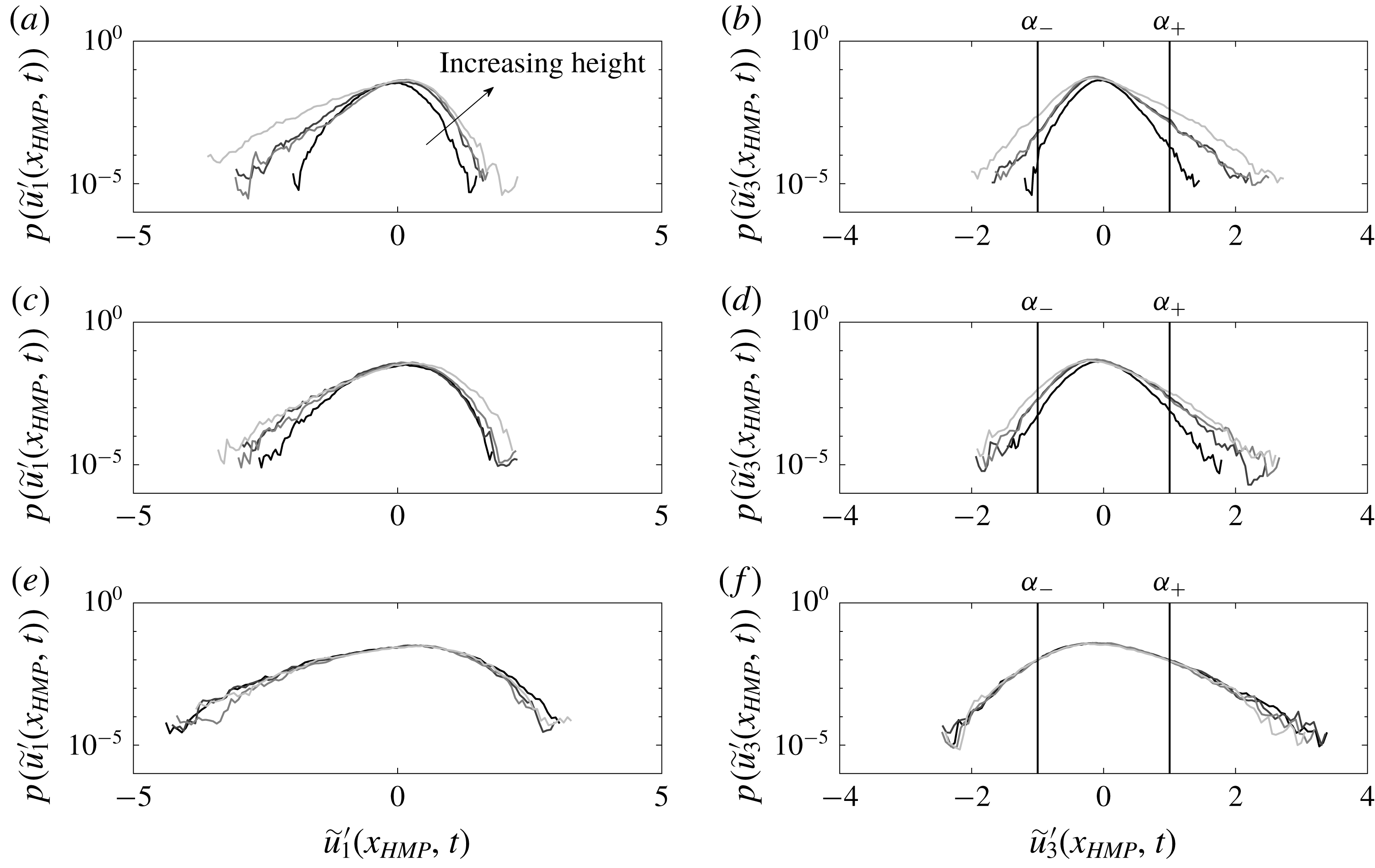
Probability density functions of fluctuating streamwise (a,c,e) and vertical (b,d,f) velocities at discrete location,
 $\boldsymbol{x}_{HMP}$
, shown in figure 1(a–f) and 2. (a,b) Show results for Cases A1, B1, C1 and D1; (c,d) show results for Cases A3, B3, C3 and D3; and (e,g) show results for Cases A6, B6, C6 and D6. In all panels, line colouring corresponds to A
 $i$
(black), B
 $i$
(dark grey), C
 $i$
(grey) and D
 $i$
(light grey), where
 $i=1$
(a,b), 3 (c,d) and 6 (e,f). Vertical lines in (b,d,f) denote thresholds,
 $\unicode[STIX]{x1D6FC}_{-}$
and
 $\unicode[STIX]{x1D6FC}_{+}$
, used during conditional sampling of flow. Annotation for direction of increasing element height,
 $h$
, added to (a), for perspective.

Figure 6 shows probability density functions (p.d.f.) of fluctuating streamwise (a,c,e) and wall-normal (b,d,f) velocity from the discrete sampling point,
 $\boldsymbol{x}_{HMP}$
, shown in figures 1(a–f) and 2. The p.d.f.s are shown for cases in the topography (a,b), transitional (c,d) and roughness (e,f) regimes, with the direction of increasing element height annotated in (a). For the canonical arrangement of turbulent channel flow over a homogeneous roughness, streamwise and wall-normal velocity skewness at the outer-layer sampling point,
 $\boldsymbol{x}_{HMP}$
, should be negative and positive, respectively (Raupach et al.
Reference Raupach, Antonia and Rajagopalan1991). This pattern is, indeed, observed for the roughness regime p.d.f.s, where the differences between cases are modest. Differences emerge at the relatively low-probability extremes of the p.d.f.s (i.e. the ‘tails’), which should be expected due to perturbations associated with the large elements. Although the p.d.f. tails are, by definition, associated with relatively lower-probability fluctuations, we direct the interested reader to table 1; the right-hand column summarizes the simulation duration via number of ‘large-eddy turnovers’,
 $TU_{0}\unicode[STIX]{x1D6FF}^{-1}\sim O(10^{3})$
. This integration time is sufficient for well resolved p.d.f.s, and stationary conditional averages, even when considering the relatively smaller subset of instants used to capture conditional averages.
In the transition and topography regime, the p.d.f.s are strikingly different: while the streamwise and wall-normal velocity fluctuations remain negatively and positive skewed, respectively, the elements now impart a dramatic influence on the velocity fluctuations.
The figure 6 p.d.f.s demonstrate the potential for system reversals – that is, events with opposite directional sign, which in this case implies the interchange between upwelling of low-momentum fluid or downwelling of high-momentum fluid. With this, and since downwelling and upwelling is a defining marker on the presence of a HMP or LMP, respectively (see figure 2
b,d,f and accompanying text), we have used the figure 6 p.d.f.s of vertical velocity to introduce thresholds for use during conditional sampling of the flow. The
 $\boldsymbol{x}_{HMP}$
marker noted on figures 1 and 2 was selected since, at this location, secondary flows associated with the roughness sublayer will have attenuated; instead, the only secondary flows present will be those related to outer-layer secondary flows. This article is concerned, specifically, with non-periodic reversals of the outer-layer secondary flows, which are driven by spatial heterogeneity of the Reynolds stresses (equation (2.1), figure 5, and accompanying text), but prone to sudden reversals. This approach will, thus, provide an aggregate view of the flow structure present during times of pronounced upwelling (
 $\tilde{u} _{3}^{\prime }(\boldsymbol{x}_{HMP},t)>\unicode[STIX]{x1D6FC}_{-}$
) or downwelling (
 $\tilde{u} _{3}^{\prime }(\boldsymbol{x}_{HMP},t)<\unicode[STIX]{x1D6FC}_{-}$
).
Conditional averaging is a popular technique for characterizing the spatial attributes of turbulence (Antonia Reference Antonia1981; Kim, Moin & Moser Reference Kim, Moin and Moser1987; Adrian Reference Adrian1988; Finnigan, Shaw & Patton Reference Finnigan, Shaw and Patton2009; Sheng, Malkiel & Katz Reference Sheng, Malkiel and Katz2009; Hutchins et al.
Reference Hutchins, Monty, Ganapathisubramani, Ng and Marusic2011; Richter & Sullivan Reference Richter and Sullivan2014; Jacob & Anderson Reference Jacob and Anderson2016). Unlike a Reynolds average, wherein the resultant quantity is based on an average over every state, a conditionally averaged quantity is based on a sub-set of all states and is predicated upon some pre-defined condition. The conditionally averaged velocity fields,
 $\widehat{\tilde{\boldsymbol{u}}}(\boldsymbol{x})/u_{\unicode[STIX]{x1D70F}}$
, are attained with the operations:
 $$\begin{eqnarray}{\displaystyle \frac{\widehat{\tilde{\boldsymbol{u}}}_{\unicode[STIX]{x1D6FC}_{-}}(\boldsymbol{x})}{u_{\unicode[STIX]{x1D70F}}}}=\left\langle \left.{\displaystyle \frac{\tilde{\boldsymbol{u}}(\boldsymbol{x},t)}{u_{\unicode[STIX]{x1D70F}}}}\right|\tilde{u} _{3}^{\prime }(\boldsymbol{x}_{HMP},t)<\unicode[STIX]{x1D6FC}_{-}\right\rangle _{N_{\unicode[STIX]{x1D6FC}_{-}}},\end{eqnarray}$$
and
 $$\begin{eqnarray}{\displaystyle \frac{\widehat{\tilde{\boldsymbol{u}}}_{\unicode[STIX]{x1D6FC}_{+}}(\boldsymbol{x})}{u_{\unicode[STIX]{x1D70F}}}}=\left\langle \left.{\displaystyle \frac{\tilde{\boldsymbol{u}}(\boldsymbol{x},t)}{u_{\unicode[STIX]{x1D70F}}}}\right|\tilde{u} _{3}^{\prime }(\boldsymbol{x}_{HMP},t)>\unicode[STIX]{x1D6FC}_{+}\right\rangle _{N_{\unicode[STIX]{x1D6FC}_{+}}},\end{eqnarray}$$
where
 $\tilde{u} _{3}^{\prime }(\boldsymbol{x}_{HMP},t)$
is the sampling quantity,
 $\unicode[STIX]{x1D6FC}_{-}$
and
 $\unicode[STIX]{x1D6FC}_{+}$
are pre-defined thresholds and
 $N_{\unicode[STIX]{x1D6FC}_{-}}$
and
 $N_{\unicode[STIX]{x1D6FC}_{+}}$
are integer number of instances at which the threshold is exceeded. Sample p.d.f.s of
 $\tilde{u} _{3}^{\prime }(\boldsymbol{x}_{HMP},t)$
for table 1 cases, and sampling thresholds, are shown in figure 6(b,d,e). For turbulence characterization, conditional sampling is appealing since turbulence structure associated with high-magnitude, low-probability events can be revealed with relative clarity (Jacob & Anderson Reference Jacob and Anderson2016).
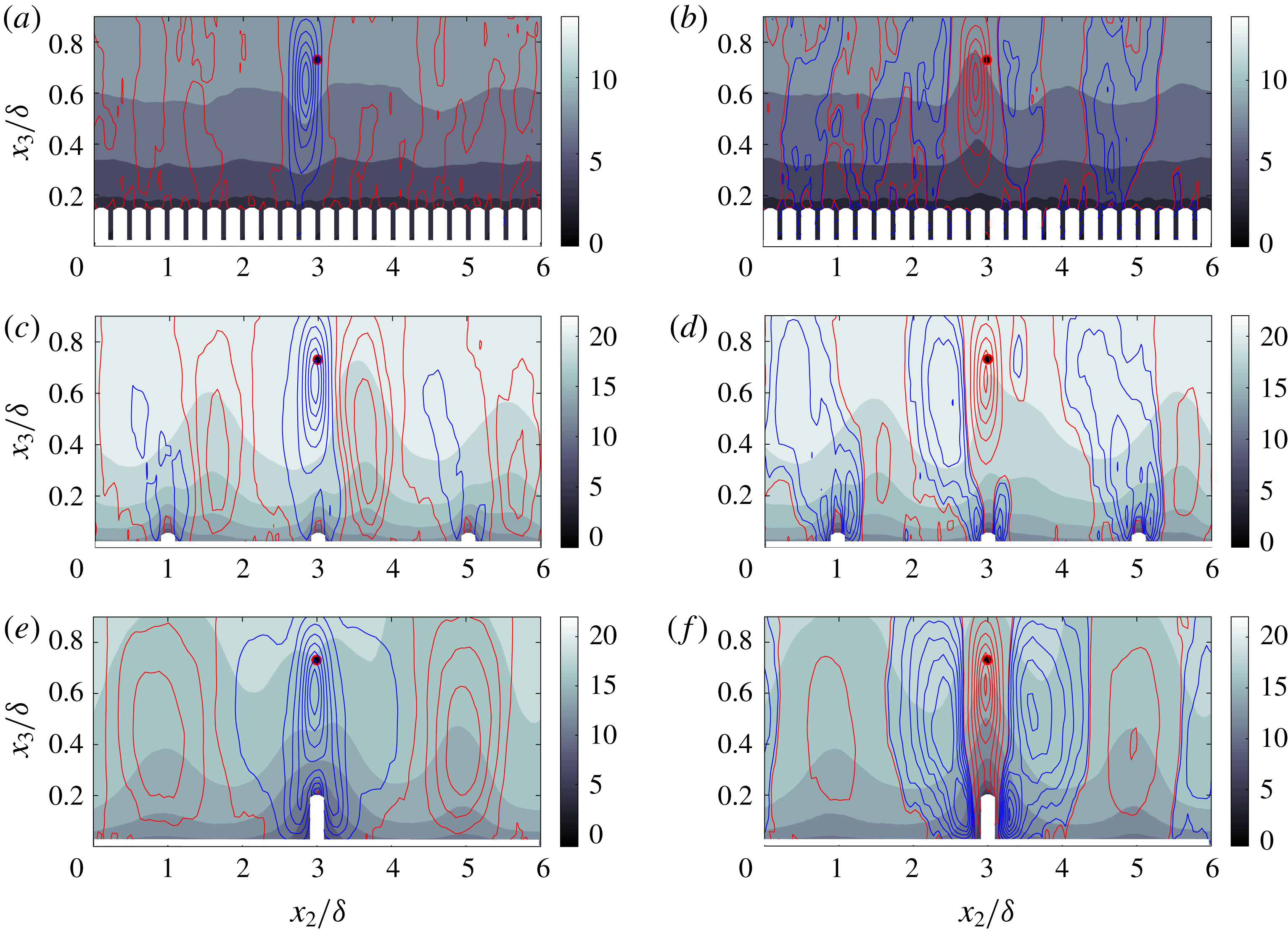
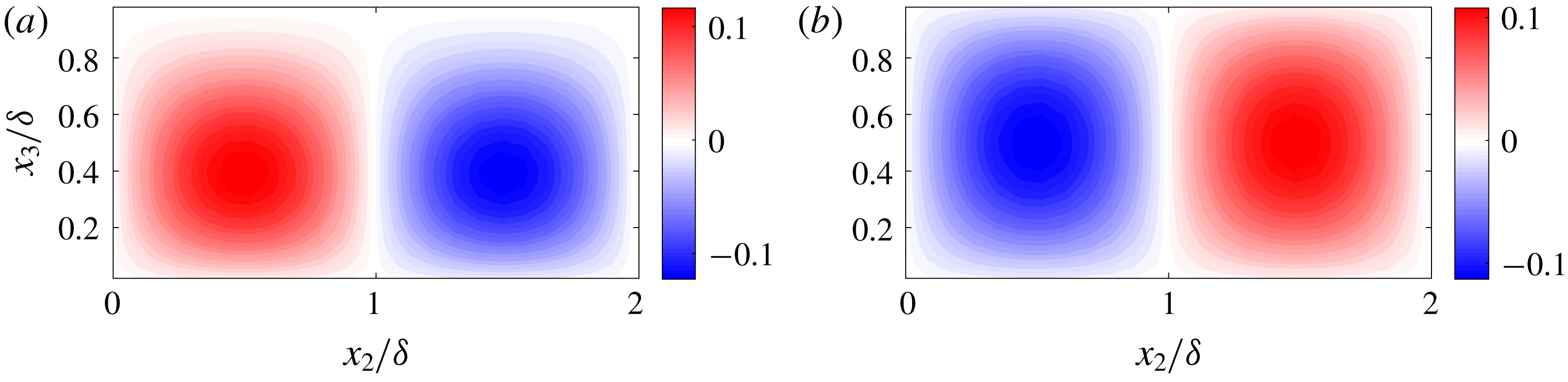
Conditionally averaged flow structure in the spanwise–wall-normal plane, based on figure 6 p.d.f.s. Colour flood contour corresponds to streamwise velocity,
 $\hat{\tilde{u} }_{1}/u_{\unicode[STIX]{x1D70F}}$
, while line contours represent positive (red) and negative (blue) components of vertical velocity,
 $\hat{\tilde{u} }_{3}/u_{\unicode[STIX]{x1D70F}}$
. (a,c,e) Correspond to flow sampling based upon
 $\tilde{u} _{3}(\boldsymbol{x}_{HMP},t)/u_{\unicode[STIX]{x1D70F}}\leqslant \unicode[STIX]{x1D6FC}_{-}$
(2.2), while (b,d,e) correspond to flow sampling based upon
 $\tilde{u} _{3}(\boldsymbol{x}_{HMP},t)/u_{\unicode[STIX]{x1D70F}}\geqslant \unicode[STIX]{x1D6FC}_{+}$
(2.3), where both thresholds are shown in figure 6(b,d,f). (a,b) Case C6; (c,d) Case A3; (d,e) Case D1.

Figure 7 shows conditionally averaged contours of streamwise velocity (colour flood), with line contours for wall-normal velocity superimposed; the wall-normal velocity contours are divided into positive (red) and negative (blue). The figure format is identical to that used for figure 2. The figures are arranged such that (a,b), (c,d) and (e,f) correspond to roughness, transitional and topography regime surfaces, respectively, while (a,c,e) and (b,d,f) show statistics for
 $\widehat{\tilde{\boldsymbol{u}}}_{\unicode[STIX]{x1D6FC}_{-}}(\boldsymbol{x})/u_{\unicode[STIX]{x1D70F}}$
and
 $\widehat{\tilde{\boldsymbol{u}}}_{\unicode[STIX]{x1D6FC}_{+}}(\boldsymbol{x})/u_{\unicode[STIX]{x1D70F}}$
, respectively.
In the roughness regime, figure 7(a,b) shows local zones of downwelling and upwelling, respectively, surrounding the sampling point, beyond which the distribution rapidly approaches a channel-like distribution above a homogeneous rough surface (i.e. sandpaper). In this sense, the upwelling and downwelling are not indications of an LMP or HMP, but rather due to the passage of coherent motions within the flow: since the flow is responding to a uniform distribution of roughness elements, roughness-driven secondary flows in the outer layer cannot form, which differs intrinsically to large-spacing cases that exhibit domain-scale Reynolds-averaged secondary cells in the outer layer (see also figure 2). As such, any domain-scale patterns of coherence for these roughness cases can only be attributed to the passage of coherent motions (Yang & Anderson Reference Yang and Anderson2017). For the large element roughness cases with
 $\unicode[STIX]{x1D6FF}/h=5$
, 6.7 or 10 (see table 1), one hesitates to attribute these to large-scale motions, since such outer-layer coherence attenuates in the presence of large elements. However, for the small element roughness cases (i.e. A5 and A6), outer layer similarity is possible and the structures could be due to the passage of large-scale motions encapsulated by hairpins. As spacing increases, however, the picture changes entirely.
Figure 7(e,f) shows
 $\widehat{\tilde{\boldsymbol{u}}}_{\unicode[STIX]{x1D6FC}_{-}}(\boldsymbol{x})/u_{\unicode[STIX]{x1D70F}}$
and
 $\widehat{\tilde{\boldsymbol{u}}}_{\unicode[STIX]{x1D6FC}_{+}}(\boldsymbol{x})/u_{\unicode[STIX]{x1D70F}}$
, respectively, which confirm that large-scale system reversals are possible. Figure 7(e), in fact, resembles the Reynolds-averaged distribution (figure 2
f), with a zone of downwelling above the element overlapping a region of streamwise momentum excess (HMP), and flanked by adjacent zones of upwelling of low-momentum fluid (i.e. an LMP). However, when (2.3) is used to compute
 $\widehat{\tilde{\boldsymbol{u}}}_{\unicode[STIX]{x1D6FC}_{+}}(\boldsymbol{x})/u_{\unicode[STIX]{x1D70F}}$
, a distinctly different pattern is found, with upwelling overlapping a
 $\unicode[STIX]{x1D6FF}$
-scale streamwise momentum deficit, adjacent to two regions of downwelling. Note, however, that even for
 $\widehat{\tilde{\boldsymbol{u}}}_{\unicode[STIX]{x1D6FC}_{+}}(\boldsymbol{x})/u_{\unicode[STIX]{x1D70F}}$
, the two adjacent zones of upwelling (i.e.
 $0.2\lesssim x_{2}/\unicode[STIX]{x1D6FF}\lesssim 1.8$
and
 $4.2\lesssim x_{2}/\unicode[STIX]{x1D6FF}\lesssim 5.8$
) remain – with structure very similar to that observed in the
 $\widehat{\tilde{\boldsymbol{u}}}_{\unicode[STIX]{x1D6FC}_{-}}(\boldsymbol{x})/u_{\unicode[STIX]{x1D70F}}$
contours. Figure 7(e,f) demonstrates that during vertical velocity excursions of relevant probability, the system can exhibit large-scale reversals from the ‘standard’ LMP/HMP distributions (Willingham et al.
Reference Willingham, Anderson, Christensen and Barros2013; Barros & Christensen Reference Barros and Christensen2014; Anderson et al.
Reference Anderson, Barros, Christensen and Awasthi2015) to element-driven upwelling (Goldstein & Tuan Reference Goldstein and Tuan1998; Vanderwel & Ganapathisubramani Reference Vanderwel and Ganapathisubramani2015; Medjnoun et al.
Reference Medjnoun, Vanderwel and Ganapathisubramani2018). The propensity for this to occur is especially relevant in the transitional regime, where the presence of both mechanisms – element-driven upwelling, and outer-layer-driven downwelling – occurs in close proximity (figure 7
c,d).
In this section, we have demonstrated that although a Reynolds-averaged direction sign emerges within the flow, large-scale reversals are possible in the roughness-driven secondary flow. This has been demonstrated in the p.d.f.s (figure 6) and conditionally averaged turbulence statistics (figure 7). We argue that these system reversals occur in a non-periodic manner; that is, when the system is projected in its underlying phase space, it does not evolve to a fixed point or limit cycle, but instead evolves chaotically; in complementary prior work, others have seen preliminary evidence suggesting this also (Vanderwel et al. Reference Vanderwel, Stroh, Kriegseis, Frohnapfel and Ganapathisubramani2019). When the secondary cells are projected upon a spatially harmonic base flow and substituted into the governing equations, we recover a system resembling the Lorenz system (Lorenz Reference Lorenz1963). In order to provide further support for this argument, however, complementary results from experimental measurement of turbulent boundary layer flow over a complex roughness with a predominant streamwise elongation are shown. Although the experimental results are derived from flow over an intrinsically different rough surfaces, we report conceptual agreement with the LES results.
2.2 Wind-tunnel experiments
In this section, we show results of experimental measurement of turbulent boundary layer flow over a complex, multiscale roughness, and a canonical smooth wall. The roughness is derived from a severely damaged gas turbine blade digital elevation model (Bons et al.
Reference Bons, Taylor, McClain and Rivir2001). The roughness has been considered in a series of articles, from efforts to establish the limits of outer-layer similarity (Wu & Christensen Reference Wu and Christensen2007, Reference Wu and Christensen2010) to, more recently, the nature of inner–outer interactions in rough-wall boundary layers (Pathikonda & Christensen Reference Pathikonda and Christensen2017). Table 2 contains salient details of the flow conditions at the measurement location, at which the boundary layer had attained self-similar conditions. In table 2, the ‘Rough-HMP’ and ‘Rough-LMP’ labels correspond to the spanwise locations denoted in figure 8(a,b) by thick black lines with the ‘HMP’ and ‘LMP’ annotation, respectively. In addition to the brief discussion of the measurement protocol described here, note that appendix B contains a comprehensive description of the flow facility. As per table 2, the high
 $Re_{\unicode[STIX]{x1D70F}}$
values for the smooth- and rough-wall boundary layers enable direct comparison with the LES datasets under dynamically similar conditions (Jimenez Reference Jimenez2004).
Results from experimental measurement of turbulent boundary layer flow over complex roughness (Bons et al.
Reference Bons, Taylor, McClain and Rivir2001) with predominant streamwise elongation (Mejia-Alvarez & Christensen Reference Mejia-Alvarez and Christensen2010). (a) Shows a colour flood contour of Reynolds-averaged streamwise velocity, with Reynolds-averaged spanwise–wall-normal velocity vectors superimposed; data retrieved from a streamwise location at which the boundary layer has attained self-similarity, and the profile beneath the contour denotes the roughness element height at the same location. (b) Shows statistics of low-pass filtered (at scale,
 $2\unicode[STIX]{x1D6FF}$
, and denoted by
 $\overline{(\ldots )}$
) streamwise average of topography,
 $\overline{\unicode[STIX]{x1D702}}/\unicode[STIX]{x1D6FF}$
(solid black line), and spanwise gradient of topographic profile,
 $\unicode[STIX]{x2202}_{2}\overline{\unicode[STIX]{x1D702}}$
(red line). In all panels, locations of high- and low-momentum pathways are denoted, while spanwise locations corresponding to measurement locations are denoted by a thick black line. Locations at which time-series measurements retrieved within HMP and LMP denoted with white arrows. Results also presented in Barros & Christensen (Reference Barros and Christensen2014).

Summary of wind-tunnel experiment attributes.

The complex roughness is multiscale, but exhibits underlying features that enable comparison against the canonical LES cases (§ 2.1). Mejia-Alvarez & Christensen (Reference Mejia-Alvarez and Christensen2010) present p.d.f.s of the spatial gradient of the figure 8(a) surface,
 $p(\unicode[STIX]{x2202}_{1}\unicode[STIX]{x1D702}(x_{1},x_{2}))$
and
 $p(\unicode[STIX]{x2202}_{2}\unicode[STIX]{x1D702}(x_{1},x_{2}))$
, where
 $\unicode[STIX]{x1D702}(x_{2},x_{3})$
is the surface height distribution; the kurtosis of
 $p(\unicode[STIX]{x2202}_{2}\unicode[STIX]{x1D702}(x_{1},x_{2}))$
far exceeded
 $p(\unicode[STIX]{x2202}_{1}\unicode[STIX]{x1D702}(x_{1},x_{2}))$
, an indication of the relative concentration of streamwise gradients about the mean (Mejia-Alvarez & Christensen Reference Mejia-Alvarez and Christensen2010, their figure 2c,d). In fact, this can be further understood when interpreted in the context of spectral density of height (Parseval’s identity). Recall that the variance of the gradient (surface slope) is derived from integration of its spectral density,
 $(\unicode[STIX]{x1D70E}^{\unicode[STIX]{x1D6FB}\unicode[STIX]{x1D702}})^{2}=\int _{2\unicode[STIX]{x03C0}/L}^{2\unicode[STIX]{x03C0}/\unicode[STIX]{x1D702}_{h}}E_{s}(k)\,\text{d}k$
, where
 $\unicode[STIX]{x1D702}_{h}$
and
 $L$
denote the cutoff wavelength and largest energy-containing wavelength of
 $\unicode[STIX]{x1D702}(x_{1},x_{2})$
, respectively,
 $k=\boldsymbol{k}\boldsymbol{\cdot }\boldsymbol{k}$
and
 $E_{s}(k)$
is spectral density of
 $\unicode[STIX]{x1D735}\unicode[STIX]{x1D702}(x_{1},x_{2})$
. Since
 $E_{s}(k)\sim k^{2}E_{h}(k)$
, where
 $E_{h}(k)$
is the spectral density of height, it follows that
 $\unicode[STIX]{x1D70E}^{\unicode[STIX]{x1D6FB}\unicode[STIX]{x1D702}}\sim (k^{2}E_{h}(k))^{1/2}$
. If
 $\unicode[STIX]{x1D702}$
is a self-similar distribution, for which the spectral density of height follows a power law,
 $E_{h}(k)\sim k^{\unicode[STIX]{x1D6FD}}$
, where
 $\unicode[STIX]{x1D6FD}$
is the spectral exponent,
 $\unicode[STIX]{x1D70E}^{\unicode[STIX]{x1D6FB}\unicode[STIX]{x1D702}}\sim k^{(1/2)(2+\unicode[STIX]{x1D6FD}_{s})}$
. Thus, that the p.d.f.s of the streamwise and spanwise gradients of the complex roughness are narrower and wider, respectively, demonstrates a relatively steeper and flatter spectral distribution, respectively.
The figure 8 complex roughness has been compared against conceptually similar results from LES on a number of previous occasions, where in all cases favourable agreement has been found (Willingham et al.
Reference Willingham, Anderson, Christensen and Barros2013; Anderson et al.
Reference Anderson, Barros, Christensen and Awasthi2015). Figure 8(a), bottom, shows a spanwise transect of the roughness height recorded at the flow measurement location. Figure 8(a), top, shows a contour of Reynolds-averaged streamwise velocity at a streamwise location at which the boundary layer has attained self-similarity. In order to provide additional detail, vectors for spanwise and wall-normal velocity have been superimposed upon the colour flood (figure originally presented in Barros & Christensen Reference Barros and Christensen2014, and included here with the permission of the authors). In the absence of spanwise surface gradients, the spanwise undulations in Reynolds-averaged velocity vanish, leaving only the wall-normal gradient (and, of course, the relatively smaller streamwise gradient). The Reynolds-averaged flow is clearly modulated by the surface characteristics, although establishing causality is not readily possible from figure 8(a) (or the height transect shown below the panel). In order to clearly demonstrate how the flow responds to salient characteristics of the surface, Barros & Christensen (Reference Barros and Christensen2014) developed the figure 8(b) surface statistics of
 $\unicode[STIX]{x1D702}$
following low-pass filtering at filter scale,
 $2\unicode[STIX]{x1D6FF}$
, which is denoted by
 $\overline{(\ldots )}$
.
The figure 8(b) profiles offer immediate insight into how the surface modulates the Reynolds-averaged flow. Considering firstly
 $\overline{\unicode[STIX]{x1D702}}/\unicode[STIX]{x1D6FF}$
, where positive and negative values represent relatively ‘more rough’ and ‘less rough’ regions of the surface, respectively, it is clear that large-scale downwelling (and streamwise momentum excesses) occurs above
 $\overline{\unicode[STIX]{x1D702}}/\unicode[STIX]{x1D6FF}>0$
. In contrast, large-scale upwelling (and streamwise momentum deficits) is positioned above regions of
 $\overline{\unicode[STIX]{x1D702}}/\unicode[STIX]{x1D6FF}<0$
– the ‘low drag’ regions. Locations of upwelling and downwelling are categorically LMPs and HMPs, respectively, and the self-organization of HMPs above the ‘high drag’ regions has been established now in a series of preceding articles (Willingham et al.
Reference Willingham, Anderson, Christensen and Barros2013; Barros & Christensen Reference Barros and Christensen2014; Anderson et al.
Reference Anderson, Barros, Christensen and Awasthi2015; see also figure 2
f and accompanying discussion). Moreover, in-depth analysis of the turbulent stress distribution for the complex roughness case demonstrated conceptual agreement with the canonical LES cases (Anderson et al.
Reference Anderson, Barros, Christensen and Awasthi2015). Nevertheless, in this section we will show evidence that within the HMP and LMP – in this case, those denoted by heavy black line in figure 8(a) – large-scale system reversals from the established Reynolds-averaged flow patterns are possible.
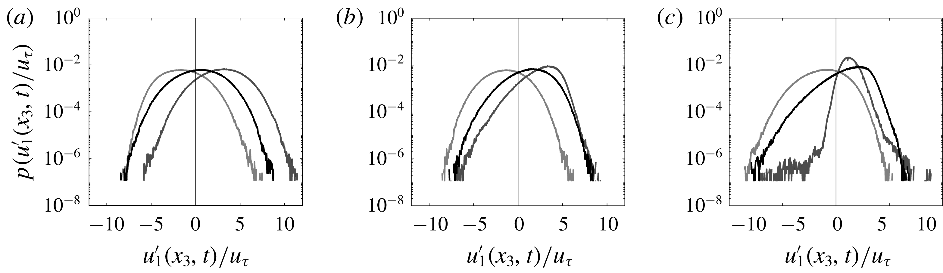
Figure 9 shows p.d.f.s of streamwise velocity fluctuations about the Reynolds-averaged velocity within the LMP and HMP:
 $$\begin{eqnarray}u_{1}^{\prime }(\boldsymbol{x},t)=u_{1}(\boldsymbol{x},t)-{\textstyle \frac{1}{2}}(\langle u_{1}\rangle _{T}(x_{1},x_{2,LMP},x_{3})+\langle u_{1}\rangle _{T}(x_{1},x_{2,HMP},x_{3})).\end{eqnarray}$$
The spanwise locations at which the time-series measurements were performed (shown in figure 8) were selected for two reasons: (i) they capture a distinct HMP and LMP; and (ii) they were sufficiently far from the tunnel side walls. The long time-series datasets were limited to a single streamwise location, two fixed spanwise locations and a series of discrete wall-normal locations (denoted by white arrows in figure 8
a,b). For this reason, subtraction of the right-hand side average in (2.4) is appealing since within a HMP and LMP,
 $\langle u_{1}^{\prime }\rangle _{T}(x_{1},x_{2,HMP},x_{3})>0$
and
 $\langle u_{1}^{\prime }\rangle _{T}(x_{1},x_{2,LMP},x_{3},t)<0$
, respectively, and thus large-scale excursions from the Reynolds-averaged flow patterns can be more readily discerned.
Probability density functions of fluctuating streamwise velocity at elevation
 $x_{3}/\unicode[STIX]{x1D6FF}=0.1$
(a), 0.2 (b) and 0.355 (c), where fluctuations are measured relative to the average velocity within the HMP and LMP (2.4) for the rough-wall cases, while fluctuations are based upon deviations about the Reynolds average for the smooth-wall case. Measurement location graphically denoted in figure 8(a). In the panels, black, grey and light grey lines correspond to measurement within turbulent boundary layer flow over a smooth wall, within a HMP and within an LMP, respectively (see table 2 for experiment details; see figure 8
a,b for visualization of measurement location).

To provide more clarity for this argument, and to cast the rough-wall results within a broader context, figure 9 shows p.d.f.s of fluctuating streamwise velocity (via (2.4)) at three outer-scaled wall-normal positions (values shown in the figure caption; profile colour coding is explained in the caption also). Salient details of the smooth-wall experiment are summarized in table 2 and appendix B. Since (2.4) is used to compute fluctuations for the rough-wall cases, the averages are shifted laterally from the true average, as expected.
The p.d.f.s further emphasize that within the location of a HMP, there is a non-negligible probability of streamwise velocity values resembling those within an LMP, and vice versa. This is true at the three sampling locations considered, all of which reside within a clearly defined HMP and LMP (see figure 8 b). In fact, the HMP and LMP p.d.f.s are negatively and positively skewed, respectively, indicative of the potential for occurrence of these reversal values. The passage of LSMs through a HMP or LMP may be capable of inducing a system reversal – such that locations of upwelling and downwelling reverse – although, in truth, to establish such causality is beyond the scope of this study. For the present section, we only wish to demonstrate that for flow over the complex roughness seen in figure 8, the Reynolds-average HMP and LMP arrangement is not stable for all time. By virtue of (2.4), the time-series measurements are able to highlight times when the streamwise velocity within a HMP (in a Reynolds-averaged sense) is comparable to the value within an LMP (again, in a Reynolds-averaged sense). This, by itself, provides support for the existence of large-scale (non-periodic) reversals to the Reynolds-averaged flow pattern.
Inclusion of the smooth-wall p.d.f. helps to indicate how an LMP and HMP alters turbulence properties (at least, at the discrete locations shown in figure 8 b). In the near-wall region (figure 9 a), the p.d.f.s are relatively similar (again note that the lateral shifting of the rough-wall p.d.f.s is a product of (2.4)), though not equivalent. The sampling point is ‘close’ to the surface, such that roughness sublayer processes could modulate the tails of the p.d.f. However, at progressively higher wall-normal locations (figure 9 b,c), the rough-wall p.d.f.s change materially. The HMP p.d.f. exhibits strong negative skewness (figure 9 b), and then is almost Gaussian (figure 9 c), while the LMP p.d.f. is less sensitive to wall-normal elevation. In a previous article, Awasthi & Anderson (Reference Awasthi and Anderson2018) found that turbulence structure within a HMP was profoundly modified, while turbulence structure within an LMP is relatively unaffected. The p.d.f.s here, shown relative to a baseline outer-scaled smooth-wall turbulent boundary layer, offer further support for this.
Since the time-series measurements within the LMP and HMP were not simultaneously recorded, the variability in
 $u_{1}^{\prime }(x_{1},x_{2,HMP},x_{3},t)$
and
 $u_{1}^{\prime }(x_{1},x_{2,LMP},x_{3},t)$
cannot be correlated. Thus, the existence of ‘cross-overs’ – transitions in the system such that downwelling and upwelling locations reverse – cannot be directly demonstrated. We once again note the results from Kevin and company, who showed the instantaneous propensity for depth-scale reversals from the Reynolds-averaged secondary flow patterns (Kevin et al.
Reference Monty, Bai, Pathikonda, Nugroho, Barros, Christensen and Hutchins2017, Reference Monty and Hutchins2019). They considered a herringbone surface for which the spanwise variability in surface drag is less obvious – at least relative to the cases considered herein – but nevertheless their results provide further support for the arguments derived from the present study. However, interpretation of these results within the broader context of the LES results certainly indicates that such reversals are possible. The experimental time series and p.d.f.s have shown how the streamwise velocity within a HMP and LMP vary in time; conditional sampling of the LES results – based on thresholds identified from p.d.f.s – shows the presence of reversals.
2.3 Chaos in roughness-driven secondary flows
The LES and experimental results provided in §§ 2.1 and 2.2, respectively, have demonstrated that the spatial patterns associated with HMPs and LMPs within the Reynolds-averaged flow can be disrupted and potentially reversed. The LES results were based on flow over a series of surfaces encompassing changes in spanwise spacing between adjacent rows of elements, and element height. The Reynolds-averaged results confirm downwelling (i.e. a HMP) above the elements, but conditional sampling of the flow showed that upwelling (and a streamwise momentum deficit) can occur too. Experimental results also showed conceptually similar processes, although owing to the inherent challenges of flow access, etc., a direct repetition of the LES post-processing analysis was not possible. Nevertheless, p.d.f.s show wide variability within the LMP and HMP, and flow states different to those exhibited within the logarithmic region of a smooth-wall turbulent boundary layer. Recent work by Kevin and company has shown that LSMs meandering through the domain can disrupt any outer-layer circulations due to spanwise surface heterogeneity (Kevin et al. Reference Monty, Bai, Pathikonda, Nugroho, Barros, Christensen and Hutchins2017, Reference Monty and Hutchins2019). In contrast, others have explored how LSMs are disrupted by secondary flows due to spanwise-surface heterogeneity (Pathikonda & Christensen Reference Pathikonda and Christensen2017; Awasthi & Anderson Reference Awasthi and Anderson2018). An interaction is undeniable.
In preceding articles by the author and company, it has been shown that the HMP and LMP are positioned such that there is a predominant downwelling onto the ‘more rough’ regions of the flow (Mejia-Alvarez & Christensen Reference Mejia-Alvarez and Christensen2010; Willingham et al. Reference Willingham, Anderson, Christensen and Barros2013; Barros & Christensen Reference Barros and Christensen2014; Anderson et al. Reference Anderson, Barros, Christensen and Awasthi2015; Yang & Anderson Reference Yang and Anderson2017). Others, however, have reported the precise opposite, where we note specifically results from Ganapathisubramani and company, who have found upwelling onto relative roughness peaks (Vanderwel & Ganapathisubramani Reference Vanderwel and Ganapathisubramani2015; Medjnoun et al. Reference Medjnoun, Vanderwel and Ganapathisubramani2018; Meyers, Ganapathisubramani & Cal Reference Meyers, Ganapathisubramani and Cal2019; Vanderwel et al. Reference Vanderwel, Stroh, Kriegseis, Frohnapfel and Ganapathisubramani2019). Results presented herein are not used to reconcile these ostensibly conflicting results; instead, we have leveraged the widely accepted result that the Reynolds-averaged flow patterns are not stable for all time. Numerical and experimental results from groups studying this problem have, indeed, all shown a propensity for system reversals. In the following section, a projection for the secondary flow – which is, itself, superimposed upon a background flow – is evaluated within the context of the governing transport equations. A series of algebraic developments yields a system of ordinary differential equations governing the evolution of time-dependent parameters used to define the secondary flow. The system resembles the Lorenz system (Saltzman Reference Saltzman1962; Lorenz Reference Lorenz1963), and time integration reveals chaotic, non-periodic orbits in phase space. This result, then, provides evidence that the reversals observed in simulations and experiments occur in a chaotic, non-periodic manner.
3 Governing equations and vortex forcing
In this section, the equations governing transport of momentum and vorticity will be revisited, following introduction of a vortex force to capture the influence of spanwise-heterogeneous surface conditions. The vortex force is inspired by a pre-existing and well established body of literature in the area of Langmuir turbulence modelling (Stokes Reference Stokes1847; Leibovich Reference Leibovich1977, Reference Leibovich1980, Reference Leibovich1983; Craik Reference Craik1985; McWilliams et al. Reference McWilliams, Sullivan and Moeng1997; Yang et al. Reference Yang, Chen, Chamecki and Meneveau2015). For the present purposes, however, the vortex force is not the product of a drift velocity and imposed wind stress, but rather an ‘inverted’ vortex velocity profile. In other work, Waleffe (Reference Waleffe1998) used a vortex force assigned to explore the underlying formation mechanisms responsible for coherent streaks in canonical wall flows. As will be comprehensively shown in the following developments, this approach imposes body forces that maintain a vortex forcing and sustain the secondary cells. Efficacy of this approach was rigorously demonstrated in Anderson et al. (Reference Anderson, Yang, Shrestha and Awasthi2018), and as such this exercise is not repeated here. Consider, firstly, the low-pass filtered momentum transport equation:
 $$\begin{eqnarray}{\displaystyle \frac{\text{D}\langle \boldsymbol{u}\rangle _{t}}{\text{D}t}}=-{\displaystyle \frac{1}{\unicode[STIX]{x1D70C}}}\unicode[STIX]{x1D735}p-\unicode[STIX]{x1D735}\boldsymbol{\cdot }\langle \unicode[STIX]{x1D64F}\rangle _{t}+\unicode[STIX]{x1D708}\unicode[STIX]{x1D6FB}^{2}\boldsymbol{u}-\boldsymbol{e}_{1}\unicode[STIX]{x1D6F1}+\langle \,\boldsymbol{f}^{\unicode[STIX]{x1D714}}\rangle _{t},\end{eqnarray}$$
where
 $\langle \ldots \rangle _{t}$
denotes filtering at the depth of the flow,
 $\unicode[STIX]{x1D6FF}$
, via convolution with the filtering kernel,
 $\langle \unicode[STIX]{x1D719}(\boldsymbol{x})\rangle _{t}=\int _{\text{d}^{3}\boldsymbol{x}}\unicode[STIX]{x1D719}(\boldsymbol{x})\star G_{\unicode[STIX]{x1D6FF}}\,\text{d}^{3}\boldsymbol{x}$
,
 $\langle \unicode[STIX]{x1D64F}\rangle _{t}=\langle \boldsymbol{u}^{\prime }\otimes \boldsymbol{u}^{\prime }\rangle _{t}$
is a turbulent stress tensor associated with sub-
 $\unicode[STIX]{x1D6FF}$
-scale eddies, which are low-pass filtered from the original quantities,
 $\boldsymbol{u}^{\prime }=\boldsymbol{u}-\langle \boldsymbol{u}\rangle _{t}$
, and
 $\unicode[STIX]{x1D6F1}=-u_{\unicode[STIX]{x1D70F}}^{2}\unicode[STIX]{x1D6FF}^{-1}\boldsymbol{e}_{1}$
is an imposed pressure gradient, where
 $u_{\unicode[STIX]{x1D70F}}$
is an imposed shear velocity (defined a priori),
 $\unicode[STIX]{x1D70C}$
is fluid density and
 $\unicode[STIX]{x1D708}$
is kinematic viscosity;
 $\boldsymbol{e}_{1}$
is the streamwise standard basis. Thus, the low-pass filter adopted here is selected to divide the constituent range of motions between attached eddies (Townsend Reference Townsend1976) and those exceeding
 $\unicode[STIX]{x1D6FF}$
, where the dynamics of the latter will be studied as it relates to modulation of the former. For these present article, these supra-
 $\unicode[STIX]{x1D6FF}$
scales are, of course, the turbulent secondary flows, which will be presumed to exhibit streamwise homogeneity. The final term on the right-hand side of (3.1) is a body force, computed here via introduction of an
 $x_{2}$
–
 $x_{3}$
dependent forcing velocity, viz.:
 $$\begin{eqnarray}\langle \,\boldsymbol{f}^{\unicode[STIX]{x1D714}}\rangle _{t}=\boldsymbol{u}^{\unicode[STIX]{x1D714}}\times \langle \unicode[STIX]{x1D74E}\rangle _{t},\end{eqnarray}$$
where
 $\langle \unicode[STIX]{x1D74E}\rangle _{t}=\unicode[STIX]{x1D735}\times \langle \boldsymbol{u}\rangle _{t}$
is the
 $\unicode[STIX]{x1D6FF}$
-averaged vorticity and
 $\boldsymbol{u}^{\unicode[STIX]{x1D714}}$
is a forcing velocity used to sustain counter-rotating vortices:
 $$\begin{eqnarray}\boldsymbol{u}^{\unicode[STIX]{x1D714}}(x_{2},x_{3},t)=\{U^{\unicode[STIX]{x1D714}}(t)g(x_{2},x_{3},t),0,0\},\end{eqnarray}$$
where
 $U^{\unicode[STIX]{x1D714}}(t)$
is a magnitude and the function,
 $g(x_{2},x_{3},t)$
, regulates the spatial distribution of the body force (discussion to follow). Equation (3.3) may be thought of as the analogue of a Stokes drift profile, but we emphasize that the functional description and spatial nature of
 $\boldsymbol{u}^{\unicode[STIX]{x1D714}}(x_{2},x_{3},t)$
is materially different. By virtue of the vortex forcing, note that
 $f_{i}^{\unicode[STIX]{x1D714}}=\unicode[STIX]{x1D716}_{ijk}\unicode[STIX]{x1D714}_{j}u_{k}^{\unicode[STIX]{x1D714}}=\{0,u_{1}^{\unicode[STIX]{x1D714}}\unicode[STIX]{x2202}_{2}u_{1},u_{1}^{\unicode[STIX]{x1D714}}\unicode[STIX]{x2202}_{3}u_{1}\}$
(i.e. the vector has zero magnitude in the streamwise direction, since only its spanwise–wall-normal components sustain counter-rotating streamwise roll cells). The streamwise component of (3.1) can be expressed as:
 $$\begin{eqnarray}{\displaystyle \frac{\text{D}\langle u_{1}\rangle _{t}}{\text{D}t}}=-{\displaystyle \frac{1}{\unicode[STIX]{x1D70C}}}\unicode[STIX]{x2202}_{1}p-\unicode[STIX]{x2202}_{i}\langle \unicode[STIX]{x1D61B}_{1i}\rangle _{t}+\unicode[STIX]{x1D708}\unicode[STIX]{x2202}_{i}^{2}\langle u_{1}\rangle _{t}-\unicode[STIX]{x1D6F1}.\end{eqnarray}$$
From (3.1), the accompanying transport equation for Reynolds-averaged vorticity is attained with the curl operation,
 $$\begin{eqnarray}{\displaystyle \frac{\text{D}\langle \unicode[STIX]{x1D74E}\rangle _{t}}{\text{D}t}}=\langle \unicode[STIX]{x1D74E}\rangle _{t}\boldsymbol{\cdot }\unicode[STIX]{x1D735}\langle \boldsymbol{u}\rangle _{t}-\unicode[STIX]{x1D735}\times (\unicode[STIX]{x1D735}\boldsymbol{\cdot }\langle \unicode[STIX]{x1D64F}\rangle _{t})+\unicode[STIX]{x1D708}\unicode[STIX]{x1D6FB}^{2}\unicode[STIX]{x1D74E}+\unicode[STIX]{x1D735}\times \langle \,\boldsymbol{f}^{\unicode[STIX]{x1D714}}\rangle _{t},\end{eqnarray}$$
where expansion of the streamwise component yields,
 $$\begin{eqnarray}{\displaystyle \frac{\text{D}\langle \unicode[STIX]{x1D714}_{1}\rangle _{t}}{\text{D}t}}=\langle \unicode[STIX]{x1D714}_{i}\rangle _{t}\unicode[STIX]{x2202}_{i}\langle u_{1}\rangle _{t}-\unicode[STIX]{x1D716}_{1qi}\unicode[STIX]{x2202}_{q}\unicode[STIX]{x2202}_{j}\langle \unicode[STIX]{x1D61B}_{ji}\rangle _{t}+\unicode[STIX]{x1D708}\unicode[STIX]{x2202}_{i}^{2}\langle \unicode[STIX]{x1D714}_{1}\rangle _{t}+\unicode[STIX]{x1D716}_{1jk}\unicode[STIX]{x2202}_{j}\langle f_{k}^{\unicode[STIX]{x1D714}}\rangle _{t}.\end{eqnarray}$$
For applications to turbulent channel and pipe flows with spanwise surface heterogeneity (owing to topographic forcing) but streamwise homogeneity, all streamwise derivatives within (3.4) and (3.6) vanish (Willingham et al.
Reference Willingham, Anderson, Christensen and Barros2013; Anderson et al.
Reference Anderson, Barros, Christensen and Awasthi2015). With this condition, we immediately deduce that the stretching and tilting term,
 $\langle \unicode[STIX]{x1D714}_{i}\rangle _{t}\unicode[STIX]{x2202}_{i}\langle u_{1}\rangle _{t}=\langle \unicode[STIX]{x1D714}_{1}\rangle _{t}\unicode[STIX]{x2202}_{1}\langle u_{1}\rangle _{t}+\langle \unicode[STIX]{x1D714}_{2}\rangle _{t}\unicode[STIX]{x2202}_{2}\langle u_{1}\rangle _{t}+\langle \unicode[STIX]{x1D714}_{3}\rangle _{t}\unicode[STIX]{x2202}_{3}\langle u_{1}\rangle _{t}$
, vanishes upon substitution of the vorticity components,
 $\langle \unicode[STIX]{x1D74E}\rangle _{t}=\{\unicode[STIX]{x2202}_{2}\langle u_{3}\rangle _{t}-\unicode[STIX]{x2202}_{3}\langle u_{2}\rangle _{t},\unicode[STIX]{x2202}_{3}\langle u_{1}\rangle _{t}-\unicode[STIX]{x2202}_{1}\langle u_{3}\rangle _{t},\unicode[STIX]{x2202}_{1}\langle u_{2}\rangle _{t}-\unicode[STIX]{x2202}_{2}\langle u_{1}\rangle _{t}\}$
. Expansion of the final right-hand side term,
 $$\begin{eqnarray}\unicode[STIX]{x1D716}_{1jk}\unicode[STIX]{x2202}_{j}\langle f_{k}^{\unicode[STIX]{x1D714}}\rangle _{t}=\unicode[STIX]{x1D716}_{1jk}\unicode[STIX]{x2202}_{j}\unicode[STIX]{x1D716}_{kpq}u_{p}^{\unicode[STIX]{x1D714}}\langle \unicode[STIX]{x1D714}_{q}\rangle _{t}=\unicode[STIX]{x1D6FF}_{1p}\unicode[STIX]{x1D6FF}_{jq}\unicode[STIX]{x2202}_{j}u_{q}^{\unicode[STIX]{x1D714}}\langle \unicode[STIX]{x1D714}_{q}\rangle _{t}-\unicode[STIX]{x1D6FF}_{1q}\unicode[STIX]{x1D6FF}_{jp}\unicode[STIX]{x2202}_{j}u_{p}^{\unicode[STIX]{x1D714}}\langle \unicode[STIX]{x1D714}_{q}\rangle _{t}=\unicode[STIX]{x2202}_{j}u_{1}^{\unicode[STIX]{x1D714}}\langle \unicode[STIX]{x1D714}_{j}\rangle _{t}-\unicode[STIX]{x2202}_{j}u_{j}^{\unicode[STIX]{x1D714}}\langle \unicode[STIX]{x1D714}_{1}\rangle _{t},\end{eqnarray}$$
simplifies greatly upon application of
 $\unicode[STIX]{x2202}_{1}(\,)=0$
, resulting finally in:
 $$\begin{eqnarray}\unicode[STIX]{x1D716}_{1jk}\unicode[STIX]{x2202}_{j}\langle f_{k}^{\unicode[STIX]{x1D714}}\rangle _{t}=U^{\unicode[STIX]{x1D714}}(\unicode[STIX]{x2202}_{3}\langle u_{1}\rangle _{t}\cdot \unicode[STIX]{x2202}_{2}g-\unicode[STIX]{x2202}_{2}\langle u_{1}\rangle _{t}\cdot \unicode[STIX]{x2202}_{3}g)=U^{\unicode[STIX]{x1D714}}J(\langle u_{1}\rangle _{t},g),\end{eqnarray}$$
where
 $U^{\unicode[STIX]{x1D714}}$
is the amplitude of the pre-defined vortex forcing model, defined here with the (3.3) model, and
 $J(f,g)=\unicode[STIX]{x2202}_{2}f\unicode[STIX]{x2202}_{3}g-\unicode[STIX]{x2202}_{3}f\unicode[STIX]{x2202}_{2}g$
is the Jacobian operator. The second right-hand side term of (3.6), herein called turbulent torque, can be expressed in two ways (Mansfield, Knio & Meneveau Reference Mansfield, Knio and Meneveau1998, Reference Mansfield, Knio and Meneveau1999). Firstly, after substitution of the components of
 $\langle \unicode[STIX]{x1D64F}\rangle _{t}$
:
 $$\begin{eqnarray}\unicode[STIX]{x1D716}_{1qi}\unicode[STIX]{x2202}_{q}\unicode[STIX]{x2202}_{j}\langle \unicode[STIX]{x1D61B}_{ji}\rangle _{t}=(\unicode[STIX]{x2202}_{2}^{2}-\unicode[STIX]{x2202}_{3}^{2})\langle \unicode[STIX]{x1D61B}_{23}\rangle _{t}+\unicode[STIX]{x2202}_{23}(\langle \unicode[STIX]{x1D61B}_{33}\rangle _{t}-\langle \unicode[STIX]{x1D61B}_{22}\rangle _{t}),\end{eqnarray}$$
where readers will quickly recognize this as the right-hand side term of (2.1), and the terms responsible for Prandtl’s secondary flows of the second kind. For the present purposes, wherein we are concerned with the scale of right-hand side terms appearing in (3.6), it is more convenient to introduce the Boussinesq model (Pope Reference Pope2000):
 $$\begin{eqnarray}\unicode[STIX]{x1D64F}=-2\unicode[STIX]{x1D708}_{t}\left(\unicode[STIX]{x1D64E}-{\textstyle \frac{2}{3}}\unicode[STIX]{x1D735}\boldsymbol{\cdot }\langle \boldsymbol{u}\rangle _{t}\unicode[STIX]{x1D739}\right)+{\textstyle \frac{2}{3}}\unicode[STIX]{x1D739}tke,\end{eqnarray}$$
where
 $\unicode[STIX]{x1D708}_{t}$
is a turbulent (eddy) viscosity,
 $\unicode[STIX]{x1D64E}=(\unicode[STIX]{x1D735}\langle \boldsymbol{u}\rangle _{t}+\unicode[STIX]{x1D735}\langle \boldsymbol{u}\rangle _{t}^{\text{T}})/2$
is the strain-rate tensor and
 $tke=\langle \boldsymbol{u}^{\prime }\boldsymbol{ : }\boldsymbol{u}^{\prime }\rangle _{t}/2$
is turbulent kinetic energy. For the present solenoidal flow,
 $\unicode[STIX]{x1D735}\boldsymbol{\cdot }\langle \boldsymbol{u}\rangle _{t}=0$
, equation (3.10) reduces to
 $\unicode[STIX]{x1D64F}=-2\unicode[STIX]{x1D708}_{t}\unicode[STIX]{x1D64E}+(2/3)\unicode[STIX]{x1D739}tke$
, and substitution into (3.9) yields the somewhat simplified expression for turbulent torque (with the caveat that
 $\unicode[STIX]{x1D708}_{t}$
must be defined a priori):
 $$\begin{eqnarray}\unicode[STIX]{x1D716}_{1qi}\unicode[STIX]{x2202}_{q}\unicode[STIX]{x2202}_{j}\unicode[STIX]{x1D61B}_{ji}=-{\textstyle \frac{1}{2}}\unicode[STIX]{x1D708}_{t}(\unicode[STIX]{x2202}_{3}^{2}\langle \unicode[STIX]{x1D714}_{1}\rangle _{t}+\unicode[STIX]{x2202}_{2}^{2}\langle \unicode[STIX]{x1D714}_{1}\rangle _{t}).\end{eqnarray}$$
Substitution of the (3.8) and (3.11) relations into (3.6) yields:
 $$\begin{eqnarray}\unicode[STIX]{x2202}_{t}\langle \unicode[STIX]{x1D714}_{1}\rangle _{t}+\langle u_{i}\rangle _{t}\unicode[STIX]{x2202}_{i}\langle \unicode[STIX]{x1D714}_{1}\rangle _{t}=(\unicode[STIX]{x1D708}+\unicode[STIX]{x1D708}_{t})\unicode[STIX]{x2202}_{i}^{2}\langle \unicode[STIX]{x1D714}_{1}\rangle _{t}+U^{\unicode[STIX]{x1D714}}J(g,\langle u_{1}\rangle _{t}).\end{eqnarray}$$
Note that, as one would anticipate, the curl of the vortex forcing term (3.2) enters only on the right-hand side of the equation governing transport of
 $\langle \unicode[STIX]{x1D714}_{1}\rangle _{t}$
, i.e.
 $$\begin{eqnarray}\unicode[STIX]{x2202}_{t}\langle \unicode[STIX]{x1D714}_{2}\rangle _{t}+\langle u_{i}\rangle _{t}\unicode[STIX]{x2202}_{i}\langle \unicode[STIX]{x1D714}_{2}\rangle _{t}=\langle \unicode[STIX]{x1D714}_{i}\rangle _{t}\unicode[STIX]{x2202}_{i}\langle u_{2}\rangle _{t}+(\unicode[STIX]{x1D708}+\unicode[STIX]{x1D708}_{t})\unicode[STIX]{x2202}_{i}^{2}\langle \unicode[STIX]{x1D714}_{2}\rangle _{t},\end{eqnarray}$$
and,
 $$\begin{eqnarray}\unicode[STIX]{x2202}_{t}\langle \unicode[STIX]{x1D714}_{3}\rangle _{t}+\langle u_{i}\rangle _{t}\unicode[STIX]{x2202}_{i}\langle \unicode[STIX]{x1D714}_{3}\rangle _{t}=\langle \unicode[STIX]{x1D714}_{i}\rangle _{t}\unicode[STIX]{x2202}_{i}\langle u_{3}\rangle _{t}+(\unicode[STIX]{x1D708}+\unicode[STIX]{x1D708}_{t})\unicode[STIX]{x2202}_{i}^{2}\langle \unicode[STIX]{x1D714}_{3}\rangle _{t},\end{eqnarray}$$
while utilization of (3.10) within (3.4) yields,
 $$\begin{eqnarray}\unicode[STIX]{x2202}_{t}\langle u_{1}\rangle _{t}+\langle u_{i}\rangle _{t}\unicode[STIX]{x2202}_{i}\langle u_{1}\rangle _{t}=-{\displaystyle \frac{1}{\unicode[STIX]{x1D70C}}}\unicode[STIX]{x2202}_{1}p+(\unicode[STIX]{x1D708}+\unicode[STIX]{x1D708}_{t})\unicode[STIX]{x2202}_{i}^{2}\langle u_{1}\rangle _{t}-\unicode[STIX]{x1D6F1}.\end{eqnarray}$$
Between (3.12), (3.13), (3.14) and (3.15), the number of unknowns is formidable, and in the following section reduction by introduction of a streamfunction will be used. Note that in all subsequent developments, since it is understood that all flow quantities have been low-pass filtered at scale,
 $\unicode[STIX]{x1D6FF}$
, the filtering nomenclature
 $\langle \ldots \rangle _{t}$
will be omitted. Note that filtering at this scale is not equivalent to Reynolds averaging, and as such time-dependence is preserved via the chaotic transience of large-scale circulations.
3.1 Reduction of unknowns and models
In order to further advance the development, the number of unknowns must be reduced. A streamfunction defining flow components in the spanwise–wall-normal plane,
 $\unicode[STIX]{x1D713}(x_{2},x_{3},t)$
, will be introduced, thereby simplifying (3.12) to (3.15), since
 $u_{2}=\unicode[STIX]{x2202}_{3}\unicode[STIX]{x1D713}$
,
 $u_{3}=-\unicode[STIX]{x2202}_{2}\unicode[STIX]{x1D713}$
and
 $\unicode[STIX]{x1D714}_{1}=-\unicode[STIX]{x1D6FB}^{2}\unicode[STIX]{x1D713}$
(where it is understood that the streamwise component of the Laplacian operator vanishes due to the streamwise-homogeneity condition). Substitution into (3.12) and (3.15) yields:
 $$\begin{eqnarray}\unicode[STIX]{x2202}_{t}(\unicode[STIX]{x2202}_{i}^{2}\unicode[STIX]{x1D713})+J(\unicode[STIX]{x2202}_{i}^{2}\unicode[STIX]{x1D713},\unicode[STIX]{x1D713})=(\unicode[STIX]{x1D708}+\unicode[STIX]{x1D708}_{t})\unicode[STIX]{x2202}_{i}^{2}(\unicode[STIX]{x2202}_{i}^{2}\unicode[STIX]{x1D713})+U^{\unicode[STIX]{x1D714}}J(u_{1},g),\end{eqnarray}$$
and
 $$\begin{eqnarray}\unicode[STIX]{x2202}_{t}u_{1}+J(u_{1},\unicode[STIX]{x1D713})=-{\displaystyle \frac{1}{\unicode[STIX]{x1D70C}}}\unicode[STIX]{x2202}_{1}p+(\unicode[STIX]{x1D708}+\unicode[STIX]{x1D708}_{t})\unicode[STIX]{x2202}_{i}^{2}u_{1}-\unicode[STIX]{x1D6F1}.\end{eqnarray}$$
The number of unknowns –
 $u_{1}$
,
 $\unicode[STIX]{x1D713}$
and
 $p$
– is substantially diminished. To further the development, it is firstly helpful to normalize the system of equations by salient parameters of the problem – shear velocity,
 $u_{\unicode[STIX]{x1D70F}}$
, flow depth,
 $\unicode[STIX]{x1D6FF}$
, and vortex forcing magnitude,
 $U^{\unicode[STIX]{x1D714}}$
. Herein, superscript
 $+$
will denote a normalized variable (although, for convenience, this superscript will be omitted in all subsequent steps for brevity). To summarize, the normalization is attained with:
 $$\begin{eqnarray}t=Hu_{\unicode[STIX]{x1D70F}}^{-1}t^{+}\quad \!u_{1}=u_{\unicode[STIX]{x1D70F}}u_{1}^{+}\quad \!\unicode[STIX]{x1D713}=u_{\unicode[STIX]{x1D70F}}H\unicode[STIX]{x1D713}^{+}\quad \!\boldsymbol{x}=\unicode[STIX]{x1D6FF}\boldsymbol{x}^{+}\quad \!u_{1}^{\unicode[STIX]{x1D714}}=U^{\unicode[STIX]{x1D714}}g\quad \!p=\unicode[STIX]{x1D70C}u_{\unicode[STIX]{x1D70F}}^{2}p^{+}\quad \!\unicode[STIX]{x1D6F1}=u_{\unicode[STIX]{x1D70F}}^{2}\unicode[STIX]{x1D6FF}^{-1}\unicode[STIX]{x1D6F1}^{+}.\end{eqnarray}$$
Upon substitution, the resultant system yields:
 $$\begin{eqnarray}\unicode[STIX]{x2202}_{t}^{+}(\unicode[STIX]{x2202}_{i}^{+,2}\unicode[STIX]{x1D713}^{+})+J^{+}(\unicode[STIX]{x2202}_{i}^{+,2}\unicode[STIX]{x1D713}^{+},\unicode[STIX]{x1D713}^{+})=({\mathcal{R}}^{-1}+{\mathcal{R}}_{t}^{-1})\unicode[STIX]{x2202}_{i}^{+,2}(\unicode[STIX]{x2202}_{j}^{+,2}\unicode[STIX]{x1D713}^{+})+{\mathcal{L}}J^{+}(g,u_{1}^{+}),\end{eqnarray}$$
and
 $$\begin{eqnarray}\unicode[STIX]{x2202}_{t}^{+}u_{1}^{+}+J^{+}(u_{1}^{+},\unicode[STIX]{x1D713}^{+})=-\unicode[STIX]{x2202}_{1}^{+}p^{+}+({\mathcal{R}}^{-1}+{\mathcal{R}}_{t}^{-1})\unicode[STIX]{x2202}_{i}^{+,2}u_{1}^{+}-\unicode[STIX]{x1D6F1}^{+}.\end{eqnarray}$$
To clarify, the pressure-gradient forcing term within (3.20) goes to unity following normalization via the linear momentum balance conditions for a channel, viz.
 $\unicode[STIX]{x1D6FF}\unicode[STIX]{x1D70C}^{-1}u_{\unicode[STIX]{x1D70F}}^{-2}\,\text{d}P_{\infty }/\text{d}x=\unicode[STIX]{x1D70F}^{w}\unicode[STIX]{x1D70C}^{-1}u_{\unicode[STIX]{x1D70F}}^{-2}=\unicode[STIX]{x1D6F1}^{+}=1$
. Within (3.19) and (3.20), we emphasize the emergence of system parameters
 ${\mathcal{R}}_{\unicode[STIX]{x1D708}}=u_{\unicode[STIX]{x1D70F}}\unicode[STIX]{x1D6FF}\unicode[STIX]{x1D708}^{-1}$
,
 ${\mathcal{R}}_{t}=u_{\unicode[STIX]{x1D70F}}\unicode[STIX]{x1D6FF}\unicode[STIX]{x1D708}_{t}^{-1}$
and
 ${\mathcal{L}}=U^{\unicode[STIX]{x1D714}}/u_{\unicode[STIX]{x1D70F}}$
, corresponding to the viscous Reynolds number, turbulent Reynolds number and a parameter loosely resembling the turbulent Langmuir number (Leibovich Reference Leibovich1983). In many engineering and geophysical flows of interest – for which the turbulent flow physics are completely dominated by inertia – it is commonplace to set
 ${\mathcal{R}}_{t}^{-1}({\mathcal{R}}_{t}{\mathcal{R}}_{\unicode[STIX]{x1D708}}^{-1}+1)\rightarrow {\mathcal{R}}_{t}^{-1}$
, although in the interest of generality we retain all terms for now and further simplify by setting
 ${\mathcal{R}}^{-1}={\mathcal{R}}_{\unicode[STIX]{x1D708}}^{-1}+{\mathcal{R}}_{t}^{-1}$
. Since all variables are now non-dimensional, the superscript
 $+$
will henceforth be omitted.
Ordinarily, unknown pressure would be assessed dynamically during direct or large-eddy simulation via computation of the divergence of (3.20) and elimination of terms with
 $\unicode[STIX]{x1D735}\boldsymbol{\cdot }\boldsymbol{u}$
. This procedure yields a Poisson equation for pressure, for which the gradients are added to (3.20) as a pressure correction that serves to preserve a solenoidal vector,
 $\unicode[STIX]{x1D735}\boldsymbol{\cdot }\boldsymbol{u}=0$
. However, in this work we will consider streamwise-homogeneous models for
 $u_{1}$
and
 $\unicode[STIX]{x1D713}$
, automatically guaranteeing conservation of mass since:
 $$\begin{eqnarray}\unicode[STIX]{x1D735}\boldsymbol{\cdot }\boldsymbol{u}=\unicode[STIX]{x2202}_{1}u_{1}+\unicode[STIX]{x2202}_{23}\unicode[STIX]{x1D713}-\unicode[STIX]{x2202}_{23}\unicode[STIX]{x1D713}=0.\end{eqnarray}$$
Under this condition, the streamwise pressure correction within (3.20) vanishes, further simplifying the system of equations and reducing the number of unknowns. This is somewhat similar to Waleffe (Reference Waleffe2001, Reference Waleffe2003), who implemented a ‘roll–streak’ or poloidal–toroidal projection of velocity within the governing momentum transport equations, thereby eliminating the pressure correction term. The need for such a projection is obviated herein by virtue of the streamwise-homogeneity condition.
Following elimination of the pressure correction, equations (3.19) and (3.20) can be solved, but direct solution is complicated by the need to compute partial derivatives in
 $t$
,
 $x_{2}$
and
 $x_{3}$
. For the Reynolds-averaged version of (3.19) and (3.20), one could quickly envision possible solutions via introduction of an appropriate similarity variable (Anderson et al.
Reference Anderson, Yang, Shrestha and Awasthi2018), but this would not capture the transient nature of domain-scale rolls in the transitional regime. As an alternative, we will instead proceed with a severely truncated projection for the large-scale secondary rolls, which will yield a prognostic description for evolution of the projection coefficients.
4 Truncated Galerkin projection
The terms
 $u_{1}$
and
 $\unicode[STIX]{x1D713}$
will be projected upon basis functions, which simplifies the eventual solution of the system. In order to mimic the presence of two domain-scale, counter-rotating rolls within the spanwise–wall-normal plane,
 $\boldsymbol{x}\in \unicode[STIX]{x1D6FA}$
, and with spatial extent
 $\{(x_{2},x_{3}):0\leqslant x_{2}\leqslant 2,0\leqslant x_{3}\leqslant 1\}$
, the following models are introduced:
 $$\begin{eqnarray}\unicode[STIX]{x1D713}(x_{2},x_{3},t)=a_{1}(t)\unicode[STIX]{x1D6FC}(x_{2},x_{3}),\end{eqnarray}$$
and
 $$\begin{eqnarray}u_{1}(x_{2},x_{3},t)=a_{2}(t)\unicode[STIX]{x1D6FD}(x_{2},x_{3})+a_{3}(t)\unicode[STIX]{x1D6FE}(x_{3}),\end{eqnarray}$$
where
 $k$
is a non-dimensional spanwise wavelength associated with the adjacent, counter-rotating rolls, and the functions,
 $\unicode[STIX]{x1D6FC}(x_{2},x_{3})$
,
 $\unicode[STIX]{x1D6FD}(x_{2},x_{3})$
and
 $\unicode[STIX]{x1D6FE}(x_{3})$
, are basis functions, not yet defined for simplicity. This base flow represents the two counter-rotating rolls, which are superimposed upon the ambient channel flow turbulence. The model for
 $\unicode[STIX]{x1D713}$
should generate two counter-rotating roll cells, while the model for
 $u_{1}$
incorporates a wall-normal gradient associated with the balance of momentum between the rolls and the wall. Although a series of different projections could have been adopted (i.e. Fourier, Chebyshev, Legendre, etc.), we found that trigonometric basis functions were satisfactory for the present study. These models offer the redeeming quality of being infinitely differentiable. In addition, a model for the vortex forcing velocity is required (3.3); for convenience, it will be shown that projection upon
 $\unicode[STIX]{x1D6FD}(x_{2},x_{3})$
(4.2) yields a well-posed vortex forcing model:
 $$\begin{eqnarray}u_{1}^{\unicode[STIX]{x1D714}}(x_{2},x_{3},t)=U^{\unicode[STIX]{x1D714}}(t)g(x_{2},x_{3})=U^{\unicode[STIX]{x1D714}}(t)\unicode[STIX]{x1D6FD}(x_{2},x_{3}).\end{eqnarray}$$
With (4.1), (4.2) and (4.3), we can return to (3.19) and (3.20). Upon substitution of (4.1), (4.2) and (4.3), equation (3.19) becomes:
 $$\begin{eqnarray}\displaystyle & & \displaystyle (\unicode[STIX]{x2202}_{2}^{2}\unicode[STIX]{x1D6FC}+\unicode[STIX]{x2202}_{3}^{2}\unicode[STIX]{x1D6FC}){\displaystyle \frac{\text{d}a_{1}}{\text{d}t}}+a_{1}^{2}([\unicode[STIX]{x2202}_{2}^{3}\unicode[STIX]{x1D6FC}+\unicode[STIX]{x2202}_{233}\unicode[STIX]{x1D6FC}]\unicode[STIX]{x2202}_{3}\unicode[STIX]{x1D6FC}-[\unicode[STIX]{x2202}_{322}^{2}\unicode[STIX]{x1D6FC}+\unicode[STIX]{x2202}_{3}^{3}\unicode[STIX]{x1D6FC}]\unicode[STIX]{x2202}_{2}\unicode[STIX]{x1D6FC})\nonumber\\ \displaystyle & & \displaystyle \quad ={\mathcal{R}}^{-1}a_{1}(\unicode[STIX]{x2202}_{2}^{4}\unicode[STIX]{x1D6FC}+2\unicode[STIX]{x2202}_{2233}\unicode[STIX]{x1D6FC}+\unicode[STIX]{x2202}_{3}^{4}\unicode[STIX]{x1D6FC})+a_{3}{\mathcal{L}}(\unicode[STIX]{x2202}_{3}\unicode[STIX]{x1D6FD}\unicode[STIX]{x2202}_{2}\unicode[STIX]{x1D6FD}a_{2}-\unicode[STIX]{x2202}_{2}\unicode[STIX]{x1D6FD}[\unicode[STIX]{x2202}_{3}\unicode[STIX]{x1D6FD}a_{2}+\unicode[STIX]{x2202}_{3}\unicode[STIX]{x1D6FE}a_{3}]).\qquad\end{eqnarray}$$
For the purpose of the present work, the following basis functions are introduced:
 $$\begin{eqnarray}\displaystyle & \unicode[STIX]{x1D6FC}(x_{2},x_{3})=\sin (k\unicode[STIX]{x03C0}x_{2})\sin (\unicode[STIX]{x03C0}x_{3}), & \displaystyle\end{eqnarray}$$
 $$\begin{eqnarray}\displaystyle & \unicode[STIX]{x1D6FD}(x_{2},x_{3})=\cos (k\unicode[STIX]{x03C0}x_{2})\sin (\unicode[STIX]{x03C0}x_{3}), & \displaystyle\end{eqnarray}$$
and
 $$\begin{eqnarray}\unicode[STIX]{x1D6FE}(x_{3})=\sin (\unicode[STIX]{x03C0}x_{3}/2).\end{eqnarray}$$
For all subsequent results,
 $k=1$
unless explicitly noted otherwise. Here
 $\unicode[STIX]{x1D6FC}(x_{2},x_{3})$
and
 $\unicode[STIX]{x1D6FD}(x_{2},x_{3})$
are doubly periodic, while
 $\unicode[STIX]{x1D6FE}(x_{2},x_{3})$
is periodic only in the spanwise direction. It follows that the second right-hand side term in (4.2) represents the profile component associated with wall-normal shear. At an arbitrary time step,
 $t_{i}$
, for which
 $a_{1}(t_{i})=1$
,
 $a_{2}(t_{i})=1$
and
 $a_{3}(t_{i})=8$
, figure 10 shows sample distributions of
 $u_{1}(x_{2},x_{3},t_{i})$
(a),
 $\unicode[STIX]{x1D714}_{1}(x_{2},x_{3},t_{i})$
(b), and
 $\unicode[STIX]{x1D716}_{1jk}\unicode[STIX]{x2202}_{j}f_{k}^{\unicode[STIX]{x1D714}}$
(c). This combination of prefactors corresponds to upwelling of low-momentum fluid in the centre of the domain (a), where the low-momentum region is flanked by counter-rotating vortices (b). Figure 10(c) shows the corresponding vortex forcing, where it is clear that the term provides and depletes
 $\unicode[STIX]{x1D714}_{1}(x_{2},x_{3},t_{i})$
within regions of
 $\unicode[STIX]{x1D714}_{1}(x_{2},x_{3},t_{i})>0$
and
 $\unicode[STIX]{x1D714}_{1}(x_{2},x_{3},t_{i})<0$
, respectively. This can be deduced from the distribution of
 $\{f_{2}^{\unicode[STIX]{x1D714}},f_{3}^{\unicode[STIX]{x1D714}}\}$
, where the force is principally ‘pumping’ fluid up and down within zones of upwelling and downwelling, respectively. Upon quick comparison with figure 2(d,f), there is certainly conceptual agreement between the LES results and those from the truncated projection.
Sample model distributions at instantaneous time,
 $t_{i}$
. (a) Colour flood:
 $u_{1}(x_{2},x_{3},t_{i})$
for
 $a_{2}(t_{i})=1$
and
 $a_{3}(t_{i})=8$
(4.2); (b) colour flood:
 $\unicode[STIX]{x1D714}_{1}(x_{2},x_{3},t_{i})=-\unicode[STIX]{x2202}_{2}^{2}\unicode[STIX]{x1D713}(x_{2},x_{3},t_{i})-\unicode[STIX]{x2202}_{3}^{2}\unicode[STIX]{x1D713}(x_{2},x_{3},t_{i})=a_{1}(t_{i})\unicode[STIX]{x03C0}^{2}(1+k^{2})\sin (\unicode[STIX]{x03C0}x_{3})\sin (k\unicode[STIX]{x03C0}x_{2})$
for
 $a_{1}(t_{i})=1$
; (c) colour flood: vortex forcing distribution,
 $\unicode[STIX]{x1D716}_{1jk}\unicode[STIX]{x2202}_{j}f_{k}^{\unicode[STIX]{x1D714}}={\mathcal{L}}J(u_{1}^{\unicode[STIX]{x1D714}},u_{1})$
for
 ${\mathcal{L}}=1$
. In (a) and (b), vectors correspond to
 $\{u_{2},u_{3}\}=\{\unicode[STIX]{x2202}_{3}\unicode[STIX]{x1D713},-\unicode[STIX]{x2202}_{2}\unicode[STIX]{x1D713}\}=\{a_{1}(t_{i})\unicode[STIX]{x03C0}\cos (\unicode[STIX]{x03C0}x_{3})\sin (k\unicode[STIX]{x03C0}x_{2}),-a_{1}(t_{i})(k\unicode[STIX]{x03C0})\sin (\unicode[STIX]{x03C0}x_{3})\cos (k\unicode[STIX]{x03C0}x_{2})\}$
for
 $a_{1}(t_{i})=1$
, while vectors in (c) denote spanwise–wall-normal components of the vortex force,
 $\{f_{2}^{\unicode[STIX]{x1D714}},f_{3}^{\unicode[STIX]{x1D714}}\}=\{u_{1}^{\unicode[STIX]{x1D714}}\unicode[STIX]{x2202}_{2}u_{1},u_{1}^{\unicode[STIX]{x1D714}}\unicode[STIX]{x2202}_{3}u_{1}\}$
, for
 $a_{2}(t_{i})=1$
,
 $a_{3}(t_{i})=8$
and
 ${\mathcal{L}}=U^{\unicode[STIX]{x1D714}}(1)/u_{\unicode[STIX]{x1D70F}}=-10$
.

The vortex forcing contribution to the balance of streamwise vorticity,
 $a_{3}{\mathcal{L}}\unicode[STIX]{x2202}_{2}\unicode[STIX]{x1D6FD}\unicode[STIX]{x2202}_{3}\unicode[STIX]{x1D6FE}$
, is further outlined here. In order to capture the modulating influence of sub-
 $\unicode[STIX]{x1D6FF}$
mixing upon the secondary cells, a modest stochastic component is added to the amplitude of the vortex forcing term. Herein,
 $$\begin{eqnarray}{\mathcal{L}}={\displaystyle \frac{U^{\unicode[STIX]{x1D714}}(t)}{u_{\unicode[STIX]{x1D70F}}}}={\displaystyle \frac{U^{\unicode[STIX]{x1D714}}}{u_{\unicode[STIX]{x1D70F}}}}(1+\unicode[STIX]{x1D702}(t)),\quad \text{where}~\unicode[STIX]{x1D702}(t)=\mathop{\sum }_{\boldsymbol{k}}f_{\boldsymbol{k}}\unicode[STIX]{x1D702}_{\boldsymbol{k}}(t)(2\unicode[STIX]{x03C0})^{-1}\exp (\text{i}\boldsymbol{k}\boldsymbol{\cdot }\boldsymbol{x}),\end{eqnarray}$$
where
 $f_{\boldsymbol{k}}$
sets the amplitude of Fourier modes over constituent wavelengths (here unity for all
 $\boldsymbol{k}$
), while
 $\langle \unicode[STIX]{x1D702}_{\boldsymbol{k}}(t)\unicode[STIX]{x1D702}_{\boldsymbol{k}}^{\prime }(t^{\prime })\rangle =\unicode[STIX]{x1D6FF}_{\boldsymbol{k}\boldsymbol{k}^{\prime }}\unicode[STIX]{x1D6FF}(t-t^{\prime })$
, thereby guaranteeing an exponent of zero upon the spectral density (i.e.
 $E_{\unicode[STIX]{x1D702}}\sim k^{0}$
, where
 $k=\boldsymbol{k}\boldsymbol{\cdot }\boldsymbol{k}$
). Nevertheless, this stochastic (in time) amplitude sets the magnitude of the harmonic (in space) vortex forcing; the figure 10(c) contour corresponds to
 ${\mathcal{L}}=1$
, demonstrating how the forcing ‘pumps’ relatively low-momentum fluid upward within low-momentum pathways.
For expedience, appendix C presents a summary of all constituent partial derivatives of the (4.5) to (4.7) harmonic functions appearing within (4.4) (and within the transport equation for
 $u_{1}$
, following substitution of the model projection). Upon substitution of partial derivatives and algebraic developments, equation (4.4) can be restated in terms of the truncated projections for
 $u_{1}$
(4.2),
 $\unicode[STIX]{x1D713}$
(4.1) and
 $u_{1}^{\unicode[STIX]{x1D714}}$
(4.3), thus:
 $$\begin{eqnarray}\unicode[STIX]{x03C0}^{2}(1+k^{2})\unicode[STIX]{x1D6FC}{\displaystyle \frac{\text{d}a_{1}}{\text{d}t}}=-{\mathcal{R}}^{-1}\unicode[STIX]{x03C0}^{4}(1+k^{2})^{2}\unicode[STIX]{x1D6FC}a_{1}+{\mathcal{L}}{\displaystyle \frac{\unicode[STIX]{x03C0}}{2}}\cos (\unicode[STIX]{x03C0}x_{3}/2)\unicode[STIX]{x1D6FC}a_{3}.\end{eqnarray}$$
In (4.9), the prefactors
 $\unicode[STIX]{x1D6FC}(x_{2},x_{3})=\sin (\unicode[STIX]{x03C0}x_{3})\sin (k\unicode[STIX]{x03C0}x_{2})$
,
 $\unicode[STIX]{x1D6FD}(x_{2},x_{3})=\sin (\unicode[STIX]{x03C0}x_{3})\cos (k\unicode[STIX]{x03C0}x_{2})$
and
 $\unicode[STIX]{x1D6FE}(x_{3})=\sin (\unicode[STIX]{x03C0}x_{3}/2)$
, were used for brevity. Note, also, that by definition,
 $J(\unicode[STIX]{x1D713},\unicode[STIX]{x2202}_{i}^{2}\unicode[STIX]{x1D713})=\unicode[STIX]{x2202}_{3}\unicode[STIX]{x1D713}(\unicode[STIX]{x2202}_{223}\unicode[STIX]{x1D713}+\unicode[STIX]{x2202}_{333}\unicode[STIX]{x1D713})-\unicode[STIX]{x2202}_{3}\unicode[STIX]{x1D713}(\unicode[STIX]{x2202}_{222}\unicode[STIX]{x1D713}+\unicode[STIX]{x2202}_{332}\unicode[STIX]{x1D713})=0$
(this result can be quickly demonstrated by substitution of the truncated Galerkin projection input functions, equation 4.5, and expansion). Recall again that appendix C contains a summary of all partial derivatives, for completeness.
Assessing first (4.9) – owing to its relative simplicity – error minimization,
 $\int _{\unicode[STIX]{x1D6FA}}\unicode[STIX]{x1D6FC}(\text{d}a_{1}/\text{d}t-\unicode[STIX]{x1D6E4})\,\text{d}\unicode[STIX]{x1D6FA}=0$
, allows for further advancement. In this argument,
 $\unicode[STIX]{x1D6FC}$
is the basis function upon which the streamfunction (and error) is projected – here truncated to first order – where
 $\unicode[STIX]{x1D6E4}$
includes all of the right-hand side terms of (4.9), and
 $\text{d}\unicode[STIX]{x1D6FA}=\text{d}x_{2}\,\text{d}x_{3}$
. Here, we integrate over the spanwise–wall-normal flow area,
 $0\leqslant x_{2}\leqslant 2/k$
and
 $0\leqslant z\leqslant 1$
, yielding:
 $$\begin{eqnarray}{\displaystyle \frac{\text{d}a_{1}}{\text{d}t}}=\unicode[STIX]{x1D6FC}_{1}a_{1}+\unicode[STIX]{x1D6FC}_{2}a_{3},\end{eqnarray}$$
where
 $\unicode[STIX]{x1D6FC}_{1}=-{\mathcal{R}}^{-1}\unicode[STIX]{x03C0}^{2}(1+k^{2})$
and
 $\unicode[STIX]{x1D6FC}_{2}={\mathcal{L}}(k/(\unicode[STIX]{x03C0}(1+k^{2})))$
. Equation (4.10) defines the evolution of the amplitude,
 $a_{1}(t)$
, used to define
 $\unicode[STIX]{x1D713}(x_{2},x_{3},t)$
(4.1). Further developments are required to attain the system equations for evolution of
 $u_{1}$
(i.e.
 $a_{2}(t)$
and
 $a_{3}(t)$
). The procedure begins by substitution of the (4.1) and (4.5) Galerkin projection models into (4.2). A series of algebraic developments result in the following:
 $$\begin{eqnarray}\displaystyle & & \displaystyle \unicode[STIX]{x1D6FD}\left[{\displaystyle \frac{\text{d}a_{2}}{\text{d}t}}-{\displaystyle \frac{k}{2}}\unicode[STIX]{x03C0}^{2}\cos (\unicode[STIX]{x03C0}x_{3}/2)a_{1}a_{3}+{\mathcal{R}}^{-1}\unicode[STIX]{x03C0}^{2}(1+k^{2})a_{2}\right]+\unicode[STIX]{x1D6FE}\left[{\displaystyle \frac{\text{d}a_{3}}{\text{d}t}}+{\mathcal{R}}^{-1}{\displaystyle \frac{\unicode[STIX]{x03C0}^{2}}{4}}a_{3}\right]\nonumber\\ \displaystyle & & \displaystyle \quad -\,k\unicode[STIX]{x03C0}^{2}\cos (\unicode[STIX]{x03C0}x_{3})\sin (\unicode[STIX]{x03C0}x_{3})a_{1}a_{2}=0.\end{eqnarray}$$
As per the development leading to (4.10), derivation of the evolution equations for
 $a_{2}$
and
 $a_{3}$
requires projection of the system upon candidate basis functions over the spanwise–wall-normal vector space. Setting the left-hand side of (4.11) equal to the symbol,
 $\unicode[STIX]{x1D6EC}(x_{2},x_{3},t)$
, two projections yield system equations for
 $a_{2}$
and
 $a_{3}$
. These are, firstly,
 $\int _{\unicode[STIX]{x1D6FA}}\unicode[STIX]{x1D6FD}(x_{2},x_{3})\unicode[STIX]{x1D6EC}(x_{2},x_{3},t)\,\text{d}\unicode[STIX]{x1D6FA}=0$
, which – after significant algebra and integration over
 $0\leqslant x_{2}\leqslant 2/k$
and
 $0\leqslant x_{3}\leqslant 1$
– reduce to:
 $$\begin{eqnarray}{\displaystyle \frac{\text{d}a_{2}}{\text{d}t}}=\unicode[STIX]{x1D6FC}_{3}a_{1}a_{3}+\unicode[STIX]{x1D6FC}_{4}a_{2},\end{eqnarray}$$
where
 $\unicode[STIX]{x1D6FC}_{3}=0.68k\unicode[STIX]{x03C0}^{2}$
and
 $\unicode[STIX]{x1D6FC}_{4}=-{\mathcal{R}}^{-1}\unicode[STIX]{x03C0}^{2}(k^{2}+1)$
. The second projection is
 $\int _{\unicode[STIX]{x1D6FA}}\sin (\unicode[STIX]{x03C0}x_{3}/2)\unicode[STIX]{x1D6EC}(x_{2},x_{3},t)\,\text{d}\unicode[STIX]{x1D6FA}=0$
, where the aforementioned algebraic and integration procedure results in:
 $$\begin{eqnarray}{\displaystyle \frac{\text{d}a_{3}}{\text{d}t}}=\unicode[STIX]{x1D6FC}_{5}a_{1}a_{2}+\unicode[STIX]{x1D6FC}_{6}a_{3},\end{eqnarray}$$
where
 $\unicode[STIX]{x1D6FC}_{5}=-0.17k\unicode[STIX]{x03C0}^{2}$
and
 $\unicode[STIX]{x1D6FC}_{6}=-{\mathcal{R}}^{-1}(1/4)\unicode[STIX]{x03C0}^{2}$
.
The (4.10), (4.12) and (4.13) system of ordinary differential equations (ODE) collectively governs the phase-space trajectory of the system parameters,
 $\boldsymbol{a}(t)$
, which can be determined via standard numerical integration schemes. The results will show that inherent nonlinearities within the system of equations – originating from the advective term in (3.19) and (3.20) – are responsible for non-periodic orbits and large-scale system reversals. Readers will quickly recognize similarities to the Lorenz system, where Reynolds number appears as a prefactor on the linear terms in all equations (Lorenz Reference Lorenz1963). Unlike the Lorenz system, however, buoyancy does not provide sustenance for the rolls (which would otherwise be measured via the Richardson number). Instead, the system is energetically sustained by the second right-hand side term in (4.10) – the vortex forcing term – and results below will show that failure to overcome the dissipative affects of turbulence will result in cessation of the cells (i.e.
 $\boldsymbol{a}(t)\rightarrow 0$
).
4.1 Boundary conditions
Within the domain,
 $\boldsymbol{x}\in \unicode[STIX]{x1D6FA}$
, limiting conditions at the domain surface,
 $\unicode[STIX]{x2202}\unicode[STIX]{x1D6FA}$
, are automatically defined through prescription of the models for
 $u_{1}$
and
 $\unicode[STIX]{x1D713}$
. At the wall,
 $x_{3}=0$
, the no-slip condition imposes
 $u_{1}(x_{1},x_{2},x_{3}=0)=u_{2}(x_{1},x_{2},x_{3}=0)=u_{3}(x_{1},x_{2},x_{3}=0)=0$
, and quick inspection of the input functions ((4.1) and (4.2)) demonstrates that the model functions comply with this condition. At the domain top,
 $x_{3}=1$
, we can deduce that
 $u_{1}(x_{2},x_{3}=1)\rightarrow \langle a_{3}\rangle _{T}$
, where
 $\langle a_{3}\rangle _{T}$
is a centreline velocity superimposed upon the ambient channel profile. This could be defined by various means – from direct a priori prescription (for modelling purposes) to prescription based upon the existence of a plane-averaged profile, in which
 $\langle a_{3}\rangle _{T}$
is presumed to be some factor of the centreline velocity,
 $\langle a_{3}\rangle _{T}=\unicode[STIX]{x1D701}U_{0}/u_{\unicode[STIX]{x1D70F}}=\unicode[STIX]{x1D701}\unicode[STIX]{x1D705}^{-1}\log (l^{-1})$
, where
 $\unicode[STIX]{x1D705}$
is the von Kármán constant and
 $l$
is a roughness length defined a priori. Note that this can be further advanced by enforcing the existence of equilibrium conditions, in which
 $u_{\unicode[STIX]{x1D70F}}$
can be defined in terms of the ambient channel forcing and
 $U_{0}/(\unicode[STIX]{x1D70F}^{w}/\unicode[STIX]{x1D70C}\unicode[STIX]{x1D6F1})^{1/2}=\unicode[STIX]{x1D705}^{-1}\log (l^{-1})$
. In addition, the flow models proposed are compliant with the channel centreline conditions,
 $u_{2}(x_{2},x_{3}=1)=u_{3}(x_{2},x_{3}=1)=0$
. Note, finally, that the standard zero-stress boundary condition typical of a channel is also attained; consider
 $\unicode[STIX]{x2202}_{3}u_{1}|_{x_{3}=1}=a_{2}\unicode[STIX]{x2202}_{3}\unicode[STIX]{x1D6FD}|_{x_{3}=1}+a_{3}\unicode[STIX]{x2202}_{3}\unicode[STIX]{x1D6FE}|_{x_{3}=1}=0$
.
In §§ 4.3 and 4.4, comprehensive results will be shown, all of which show that the system makes predictions consistent with physical expectations.
4.2 Numerical integration
Equations (4.10), (4.12) and (4.13) form a dynamical system,
 $$\begin{eqnarray}{\displaystyle \frac{\text{d}\boldsymbol{a}(t)}{\text{d}t}}=\boldsymbol{f}(x_{1},x_{2},\ldots ,x_{N})\quad \text{where}~\boldsymbol{a}(t)=\{a_{1}(t),a_{2}(t),a_{3}(t)\}~\text{and}~t\in [0,T],\end{eqnarray}$$
where
 $x_{N}$
parameters are not to be confused with the Cartesian spatial coordinates used hitherto, and
 $T$
denotes the integration period. Time integration of (4.14) predicts the phase-space trajectory (orbit) of system,
 $\boldsymbol{a}(t)$
. In this work, explicit forward Euler time integration is used to advance the system:
 $$\begin{eqnarray}\boldsymbol{a}(t+\unicode[STIX]{x1D6FF}t)=\boldsymbol{a}(t)+\unicode[STIX]{x1D6FF}t\boldsymbol{f}(x_{1},x_{2},\ldots ,x_{N})\quad \text{and}\quad t\in [0,T],\end{eqnarray}$$
where low-amplitude white noise is used to define initial conditions for the system,
 $\boldsymbol{a}(t=0)$
, as summarized in table 3. Note that the addition of unity to
 $a_{2}(0)$
is desirable, since this helps to initiate the system from a location in close proximity to a saddle node (results to follow). Table 3 contains a summary of cases, where for the present study we will quantify the system response to variable
 ${\mathcal{R}}$
, for constant
 ${\mathcal{L}}$
. Of course, further parameter variation is possible, but for the present article this range captures the values needed to attain chaotic orbits in the system. Similarly, the non-dimensional time step and non-dimensional integration time are provided, for reference. We will show that the system trajectory exhibits acceleration, and further generalizations could be adopted with local time steps, etc. but again such efforts would be superfluous to the core topic of this paper.
In the following sections, a series of results from (4.15) will be shown, which will highlight results from the system. In § 4, we will show instantaneous and Reynolds-averaged system results. In §§ 4.3 and 4.4, a series of scaling arguments for the magnitude of the Reynolds-averaged system parameters,
 $\langle \boldsymbol{a}(t)\rangle _{T}$
, are proposed, which provide further insights on how the intensity of streamfunction and streamwise velocity associated with the secondary cells should vary with system parameters. These results are used to recover scaling arguments on the intensity of compensated circulation, which agree with preceding results. Section 6 demonstrates recovery of the
 $tke$
imbalance arguments sustaining the Reynolds-averaged secondary flows, following substitution of the (4.15) model inputs. Finally, in § 7, Poincaré projection is used to identify sub-critical (i.e. dissipative system states,
 $\unicode[STIX]{x1D735}\boldsymbol{\cdot }\boldsymbol{a}<0$
) and conservative system forcing conditions, and to identify the fractal dimension (geometry) of the resultant attractor.
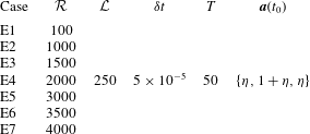
4.3 Results: non-periodic phase-space trajectories in governing equations
In order to demonstrate the potential for chaotic orbits from the system of ODEs, this section presents phase-space orbits of target cases in table 3. The cases capture parameter combinations corresponding to dissipative and conservative orbits,
 $\unicode[STIX]{x1D735}\boldsymbol{\cdot }\boldsymbol{a}<0$
and
 $\unicode[STIX]{x1D735}\boldsymbol{\cdot }\boldsymbol{a}\approx 0$
, respectively, where the system conditions dictate the rate at which dissipative systems tend toward the fixed point,
 $\boldsymbol{a}(t)=0$
. Figures 11 and 12 show a series of phase-space orbits for increasing inertial conditions. As per table 3, the orbits are all initiated from approximately the same phase-space location (the addition of low-amplitude noise,
 $\unicode[STIX]{x1D702}$
, prevents initiation from precisely the same location, although the differences are negligible).


For the weakest inertial conditions – Case E1, figure 11 – it is clear that the system is quickly overwhelmed by dissipation, as the orbit (a) amplitude quickly decreases while the system oscillates toward the origin (fixed point). The origin is a trivial fixed point, since it corresponds to a case for which no secondary circulations exist within the domain. Physically, this case corresponds to flow over a homogeneous roughness, for which there is no driving mechanism present to sustain roughness-driven secondary circulations. Gradual attenuation of the system is more clearly visible from the figure 11(b,c,d) time-series visualization, which shows how over-damping of the system suppresses its orbit amplitude (bearing resemblance to a damped sine wave). In fact, during early times, there are signs of chaotic orbits – most clearly visible in figure 11(d) for
 $tU_{0}\unicode[STIX]{x1D6FF}^{-1}\lesssim 3$
, but these oscillations are quickly damped as the system tends toward the origin. In a later section, we will demonstrate that these conditions correspond to dissipative systems (i.e.
 $\unicode[STIX]{x1D735}\boldsymbol{\cdot }\boldsymbol{a}<=0$
).
Increasing the inertial conditions by an order of magnitude helps to preserve oscillations within the system, as can be seen in figure 12 for Case E7 (
 ${\mathcal{R}}=4000$
). Unlike for
 ${\mathcal{R}}=100$
(figure 11), here the phase-space orbit now exhibits chaotic reversals for all time, which thus corresponds to a conservative system (i.e.
 $\unicode[STIX]{x1D735}\boldsymbol{\cdot }\boldsymbol{a}\approx =0$
). The attractor is shown in figure 12(a), where the perspective angle highlights orbits passing in close proximity to the saddle, and the occurrence of system reversals. The time-series evolution of parameters (figure 12
b,c,d) confirms the conservative nature of the system for
 ${\mathcal{R}}=4000$
, where large-scale variability in the system occurs in a non-periodic manner. In other testing, we have explored the limits upon continuous increases in
 ${\mathcal{R}}=4000$
. For
 ${\mathcal{R}}\gtrsim O(10^{4})$
, the system is unstable, with amplitude magnitudes continuing to increase before diverging rapidly to unphysical values.
In separate testing for intermediate inertial conditions (i.e.
 $10^{2}\lesssim {\mathcal{R}}\lesssim \times 10^{3}$
), we show monotonic increase in the duration over which the system exhibits chaotic evolution with increasing
 ${\mathcal{R}}$
. However, in these intermediate cases (Cases E1 to E5 in table 3), the system is always overwhelmed by dissipation such that the evolution is ultimately dissipative. In these intermediate cases, the orbit resembles those shown for Cases E1 and E7 (figures 11 and 12, respectively) – i.e. two limit cycles, connected at a saddle node at which orbit reversals occur – but the amplitude always tends to zero. We consistently found that
 ${\mathcal{R}}\gtrsim 3.5\times 10^{3}$
is required for conservative system evolution. For brevity, visualization of system orbit for these intermediate cases are now shown, although we note that this topic is revisited in § 7.
In order to summarize the system dynamics more succinctly, figure 13 shows an idealized sketch of system orbits in close proximity to the saddle seen on figure 12(a). As is depicted in the figure, orbits adjacent to the saddle point are considered stable, in the sense that they remain upon a limit cycle-like trajectory, and idealized boundaries demarcating the stable and unstable trajectories are denoted (orange and blue). Orbits residing in the stable regime eventually approach the saddle node from within the unstable region of the phase space (top and bottom), and in doing so the systems undergo global reversals. In the context of the LES and experimental results, such reversals correspond to the propensity of the systems to instantaneously transition between both downwelling and upwelling (i.e. between a HMP and LMP, respectively). The figure also includes idealized sampling points denoting locations where the system orbit is coincident with a plane parallel to the
 $a_{2}{-}a_{3}$
plane, and placed at
 $a_{3}=0$
. By sampling a large collection of these points as the system evolves, a Poincaré projection can be attained, which provides additional insight on the dissipative or conservative nature of the system and the system fractal dimension (attractor geometry).
Sketch of saddle point and idealized stable (grey) and unstable (black) phase-space trajectories. Orange and blue lines demarcate idealized boundary between trajectories likely to remain stable, and those corresponding to a system reversal. Shown also are idealized Poincaré projection points based upon an
 $a_{1}{-}a_{2}$
projection plane.

As a final assessment of the system dynamics, figure 14 shows the phase-space orbit for Case E6. Unlike the preceding figures, however, here we have added colour-coded data points at each discrete position on the orbit. The colour code is based upon the ‘system velocity’:
 $$\begin{eqnarray}\boldsymbol{u}_{s}(t)={\displaystyle \frac{\text{d}\boldsymbol{a}(t)}{\text{d}t}}\approx \unicode[STIX]{x1D6FF}t^{-1}\{a_{1}(t)-a_{1}(t-\unicode[STIX]{x1D6FF}t),a_{2}(t)-a_{2}(t-\unicode[STIX]{x1D6FF}t),a_{3}(t)-a_{3}(t-\unicode[STIX]{x1D6FF}t)\},\end{eqnarray}$$
where the error terms are presumed small and not consequential to the scientific deductions to be drawn from the present results. We then compute the magnitude,
 $\boldsymbol{u}_{S}\boldsymbol{\cdot }\boldsymbol{u}_{S}$
, which is used to select the symbol colour at each orbit point (warmer colours denote faster evolution, light grey highlights slowest points in orbit). This approach is helpful in terms of understanding where the orbits are accelerating and decelerating. It is clear from figure 14 that the orbit advances fastest in the outermost (in
 $a_{3}$
) regions of the phase space. The orbit decelerates as it approaches the saddle node, at which point the trajectory and ambient stochastic noise dictate the transition from stable to unstable orbit. Following this, the system rapidly accelerates as it moves outward from the saddle node.
Evolution of dynamical system composed of (4.10), (4.12) and (4.13), for
 ${\mathcal{L}}=250$
and
 ${\mathcal{R}}=3500$
(Case E6; table 3). Here, phase-space system evolution at discrete locations is colour-coded based upon ‘system velocity’ (4.16), which graphically reveals the rate of system evolution. Here, the inner product is computed,
 $\boldsymbol{u}_{S}\boldsymbol{\cdot }\boldsymbol{u}_{S}$
, and hotter colours correspond to the largest values of
 $\boldsymbol{u}_{S}\boldsymbol{\cdot }\boldsymbol{u}_{S}$
.

Inspection of the figure 12(a) orbit demonstrates some similarities and differences with the Lorenz system. Of course, as was shown in § 4, the system of ODEs differ intrinsically to the Lorenz system, guaranteeing different orbits. In the Lorenz system, a constant heat flux drives a constant rise in temperature, which explains why
 $Z(t)$
– the counterpart to
 $a_{3}(t)$
in the present system – is always positive. Here, the system is predicated upon the balance of linear momentum associated with the large-scale secondary rolls. Yet the system predicts non-periodic transitions from states resembling that observed in figure 10 – a central LMP, flanked by adjacent HMPs – to a system with a central HMP and flanked by adjacent LMPs. These transitions induce differing net momentum fluxes, such that
 $a_{3}(t)$
cannot be positive for all times. Nevertheless, we will show that when the base flow is superimposed upon a canonical logarithmic profile – thus attaining the entire Reynolds-averaged flow – realistic profiles are recovered.
4.4 Results: Reynolds-averaged statistics
This section presents a series of Reynolds-averaged turbulence statistics based upon a posteriori outputs from the (4.15) system. The results are selected to demonstrate that realistic predictions are attained from the model. Recall that the system captures the large-scale (i.e. supra-
 $\unicode[STIX]{x1D6FF}$
) rolls, and not the entire flow. For this reason, an additional logarithmic profile is added to the streamwise velocity base flow:
 $$\begin{eqnarray}\langle u_{1}\rangle _{T}(x_{2},x_{3})=\langle a_{2}\rangle _{T}\cos (k\unicode[STIX]{x03C0}x_{2})\sin (\unicode[STIX]{x03C0}x_{3})+\langle a_{3}\rangle _{T}\sin (\unicode[STIX]{x03C0}x_{3}/2)+\unicode[STIX]{x1D705}^{-1}\log \left({\displaystyle \frac{x_{3}}{l}}\right),\end{eqnarray}$$
where
 $\unicode[STIX]{x1D705}=0.4$
is the von Kármán constant and
 $l/\unicode[STIX]{x1D6FF}=10^{-4}$
is a pre-defined aerodynamic roughness length. This logarithmic profile captures the wall-normal profile due to sub-
 $\unicode[STIX]{x1D6FF}$
attached eddies, which were low-pass filtered from both variables before the development began. The first and second right-hand side terms within (4.17) represent the streamwise velocity distribution due to the turbulent secondary flows, both of which are additively combined with the logarithmic profile to capture the entire distribution.
Figure 15 shows Reynolds-averaged colour flood contours of streamwise velocity (a), and streamwise vorticity,
 $\langle \unicode[STIX]{x1D714}_{1}\rangle _{T}=-\unicode[STIX]{x1D6FB}^{2}\langle \unicode[STIX]{x1D713}\rangle _{T}$
(b). Superimposed upon both panels is a vector map for the spanwise and wall-normal velocity components. Results are shown for Case E6 (table 3), for which
 ${\mathcal{R}}=3500$
. As established in the preceding section, this Reynolds number is sufficient for conservative evolution of the system and the preservation of chaotic oscillations.
The
 $\langle u_{1}\rangle _{T}$
contour confirms that the model predicts a central LMP – evidenced by a pronounced plume of relatively low-momentum fluid at
 $x_{2}/\unicode[STIX]{x1D6FF}=1$
, and flanked by adjacent counter-rotating cells. By superimposing the vector map for the spanwise and wall-normal velocity components, the locations of upwelling and downwelling can be immediately visualized – in this case, upwelling and downwelling occurs within the LMP and adjacent HMPs, respectively, in precisely the same fashion observed from the LES and experimental results (§§ 2.1 and 2.2, respectively).
Figure 15(b) shows a corresponding contour of streamwise vorticity. To some extent, the distribution is evidenced from inspection of the vector field, but nevertheless the figure confirms that the rotational sign of the secondary rolls is such that positive and negative streamwise vorticity flanks the central LMP, as seen in the figure. Since the
 $x_{1}$
dimension is aligned in the ‘out of page’ direction, the sign of
 $\langle \unicode[STIX]{x1D714}_{1}\rangle _{T}$
is correct.
Reynolds-averaged flow from numerical solution of (4.10), (4.12) and (4.13) system. (a) Colour flood shows streamwise velocity with
 $\langle a_{2}\rangle _{T}$
and
 $\langle a_{3}\rangle _{T}$
in (4.2), while in (b) colour flood shows streamwise vorticity,
 $\langle \unicode[STIX]{x1D714}_{1}\rangle _{T}=-\unicode[STIX]{x1D6FB}^{2}\langle \unicode[STIX]{x1D713}\rangle _{T}$
, for
 $\langle a_{1}\rangle _{T}$
in (4.1). In (a) a logarithmic profile accounting for the background, ambient shear associated with the channel flow has been added (4.17). In both panels, the vector map is spanwise–wall-normal velocity,
 $\{\unicode[STIX]{x2202}_{3}\langle \unicode[STIX]{x1D713}\rangle _{T},-\unicode[STIX]{x2202}_{2}\langle \unicode[STIX]{x1D713}\rangle _{T}\}$
, for
 $\langle a_{1}\rangle _{T}$
in (4.1). Result is shown for Case E6.

Figure 16(a) shows vertical profiles of Reynolds-averaged streamwise velocity, retrieved from transects corresponding to an LMP and HMP in figure 15(a) (i.e. from
 $x_{2}/\unicode[STIX]{x1D6FF}\approx 1$
and
 $x_{2}/\unicode[STIX]{x1D6FF}\approx 0$
, respectively). The HMP and LMP are denoted by black and grey, respectively, while the additional logarithmic profile (third right-hand side term in (4.17)) is denoted by dashed black profile. For the same system conditions, figure 16(b) shows Reynolds-averaged vertical velocity at spanwise locations equivalent to the locations at which the figure 16(a) profiles were retrieved, with the canonical profile,
 $\langle u_{3}\rangle _{T}/u_{\unicode[STIX]{x1D70F}}=0$
, included for reference (dashed black). The profiles exhibit physically sensible trends. Owing to the vertical trends within the profiles, the wall-normal gradient within the HMP exceeds the corresponding value within an LMP. This can be understood by the added drag beneath a HMP (Anderson et al.
Reference Anderson, Barros, Christensen and Awasthi2015). The vertical velocity profiles are consistent with the position of downwelling and upwelling within a HMP and LMP, respectively. The profiles also agree with the profiles from LES (figure 3), especially for the smallest element height cases (i.e. Case A1).
Reynolds-averaged vertical profile of streamwise velocity computed with (4.17) (a), and vertical velocity (b), for
 $\langle a_{2}\rangle _{T}=2$
and
 $\langle a_{3}\rangle _{T}=0.02$
, at discrete spanwise locations corresponding to an LMP (grey) and HMP (black) in figure 15(a). In (a,b), dashed black profiles represent logarithmic base flow for
 $l/\unicode[STIX]{x1D6FF}=10^{-4}$
(i.e. third right-hand side term in (4.17)), and canonical channel profile,
 $\langle u_{3}\rangle _{T}/u_{\unicode[STIX]{x1D70F}}=0$
, respectively.

Since spatial heterogeneity of the Reynolds stresses is foremost in the sustenance of the present turbulent secondary flows – Prandtl’s secondary flow of the second kind, equation (2.1) – it is of interest here to consider the spatial distributions of turbulent stresses from the dynamical system. Fortunately, this can be readily accomplished using the Boussinesq assumption (equation (3.10), Pope Reference Pope2000), and the base flow projections based upon a posteriori Reynolds-averaged system parameters,
 $\langle \boldsymbol{a}\rangle _{T}$
. Only one component of
 $\unicode[STIX]{x1D64F}$
cannot be computed using the present projections,
 $\unicode[STIX]{x1D61B}_{11}$
, which is due to the streamwise-homogeneity conditions. Nevertheless, the other components can be found readily, viz.:
 $$\begin{eqnarray}\displaystyle & \langle \unicode[STIX]{x1D61B}_{12}\rangle _{T}=-{\mathcal{R}}^{-1}\unicode[STIX]{x2202}_{2}\langle u_{1}\rangle _{T}=k\unicode[STIX]{x03C0}{\mathcal{R}}^{-1}\sin (k\unicode[STIX]{x03C0}x_{2})\sin (\unicode[STIX]{x03C0}x_{3})\langle a_{2}\rangle _{T} & \displaystyle\end{eqnarray}$$
 $$\begin{eqnarray}\displaystyle \langle \unicode[STIX]{x1D61B}_{13}\rangle _{T} & = & \displaystyle -{\mathcal{R}}^{-1}\unicode[STIX]{x2202}_{3}\langle u_{1}\rangle _{T}=-{\mathcal{R}}^{-1} [\langle a_{2}\rangle _{T}\unicode[STIX]{x03C0}\cos (k\unicode[STIX]{x03C0}x_{2})\cos (\unicode[STIX]{x03C0}x_{3})\nonumber\\ \displaystyle & & \displaystyle +\,(\unicode[STIX]{x03C0}/2)\langle a_{3}\rangle _{T}\cos (\unicode[STIX]{x03C0}x_{3}/2)\!]\end{eqnarray}$$
 $$\begin{eqnarray}\displaystyle & \langle \unicode[STIX]{x1D61B}_{23}\rangle _{T}={\mathcal{R}}^{-1}(\unicode[STIX]{x2202}_{2}^{2}\langle \unicode[STIX]{x1D713}\rangle _{T}-\unicode[STIX]{x2202}_{3}^{2}\langle \unicode[STIX]{x1D713}\rangle _{T})={\mathcal{R}}^{-1}\unicode[STIX]{x03C0}^{2}\langle a_{1}\rangle _{T}(k^{2}-1)\sin (k\unicode[STIX]{x03C0}x_{2})\sin (\unicode[STIX]{x03C0}x_{3})\qquad & \displaystyle\end{eqnarray}$$
 $$\begin{eqnarray}\displaystyle & \langle \unicode[STIX]{x1D61B}_{22}\rangle _{T}-\frac{2}{3}tke=-2{\mathcal{R}}^{-1}\unicode[STIX]{x2202}_{23}\langle \unicode[STIX]{x1D713}\rangle _{T}=-2{\mathcal{R}}^{-1}k\unicode[STIX]{x03C0}^{2}\langle a_{1}\rangle _{T}\cos (k\unicode[STIX]{x03C0}x_{2})\cos (\unicode[STIX]{x03C0}x_{3}), & \displaystyle\end{eqnarray}$$
and
 $$\begin{eqnarray}\langle \unicode[STIX]{x1D61B}_{33}\rangle _{T}-{\textstyle \frac{2}{3}}tke=2{\mathcal{R}}^{-1}\unicode[STIX]{x2202}_{23}\langle \unicode[STIX]{x1D713}\rangle _{T}=2{\mathcal{R}}^{-1}k\unicode[STIX]{x03C0}^{2}\langle a_{1}\rangle _{T}\cos (k\unicode[STIX]{x03C0}x_{2})\cos (\unicode[STIX]{x03C0}x_{3}).\end{eqnarray}$$
Substitution of
 $\langle \boldsymbol{a}\rangle _{T}$
into (4.18) to (4.22) yields the turbulent stress distributions. Note that for
 $k=1$
, equation (4.20) would indicate that
 $\unicode[STIX]{x1D61B}_{23}=0$
. In order to circumvent this, however, we selected
 $k=0.98$
for this case, which enables non-zero stresses.
Reynolds-averaged deviatoric turbulent stresses:
 $\langle \unicode[STIX]{x1D61B}_{12}\rangle _{T}$
(a, equation (4.18)),
 $\langle \unicode[STIX]{x1D61B}_{13}\rangle _{T}$
(b, equation (4.19)),
 $\langle \unicode[STIX]{x1D61B}_{23}\rangle _{T}$
(c, equation (4.20)),
 $\langle \unicode[STIX]{x1D61B}_{22}\rangle _{T}-(2/3)tke$
(d, equation (4.21)) and
 $\langle \unicode[STIX]{x1D61B}_{33}\rangle _{T}-(2/3)tke$
(e, equation (4.22)). Cases shown are for
 ${\mathcal{R}}=3500$
and
 $\langle \boldsymbol{a}\rangle _{T}=\{2,2,0.02\}$
.

The turbulent stresses are shown in figure 17, for
 ${\mathcal{R}}=3500$
and Reynolds-averaged system parameter values summarized in the figure caption. Note, again, that these are only the stresses associated with the base flow, and as such direct comparison with the figure 5 contours is not possible. Nevertheless, important conclusions can be drawn from inspection of the contours. Figure 17(a,b,c) corresponds to shear-stress components
 $\unicode[STIX]{x1D61B}_{12}$
,
 $\unicode[STIX]{x1D61B}_{13}$
and
 $\unicode[STIX]{x1D61B}_{23}$
, respectively, where the distributions can be readily interpreted in the context of the underlying flow. Since
 $\unicode[STIX]{x1D61B}_{12}$
is developed by the negative of spanwise gradients in
 $u_{1}$
((4.18) and figure 15
a), the central LMP and adjacent HMPs necessitate the positive–negative distribution seen in figure 17(a).
Figure 17(b) shows the distribution of
 $\unicode[STIX]{x1D61B}_{13}$
. We again emphasize that this distribution corresponds to the base flow projection – not the total – but nonetheless
 $\unicode[STIX]{x1D61B}_{13}$
confirms a relative excess and deficit in turbulent stresses beneath the central LMP and lateral HMPs, respectively. This result is conceptually identical to prior results from this problem – indeed, Anderson et al. (Reference Anderson, Barros, Christensen and Awasthi2015) show shear-normalized streamwise–wall-normal surface stress in the spanwise direction, and results confirmed elevated stresses beneath a HMP. This can be understood, too, in the context of figure 16, since the wall-normal gradient of
 $\langle u_{1}\rangle _{T}$
is larger within a HMP, relative to an LMP.
As per (2.1), the distributions of
 $\unicode[STIX]{x1D61B}_{12}$
and
 $\unicode[STIX]{x1D61B}_{13}$
do not actually contribute to the balance of streamwise vorticity. However, the second-order spatial derivatives of
 $\unicode[STIX]{x1D61B}_{23}$
constitute the shear-stress contribution to sustenance of
 $\langle \unicode[STIX]{x1D714}_{1}\rangle _{T}$
, and figure 17(c) shows non-zero variability in
 $x_{2}$
and
 $x_{3}$
(in fact, as per (4.20), the stress is projected upon the basis function,
 $\unicode[STIX]{x1D6FC}(x_{2},x_{3})$
, equation (4.5), but scaled by different amplitudes). Similarly, figure 17(c,d) shows the distributions of
 $\unicode[STIX]{x1D61B}_{22}$
and
 $\unicode[STIX]{x1D61B}_{33}$
, respectively, and (2.1) indicates that the difference,
 $\unicode[STIX]{x1D61B}_{22}-\unicode[STIX]{x1D61B}_{23}$
, regulates the normal stress contribution to
 $\langle \unicode[STIX]{x1D714}_{1}\rangle _{T}$
. The normal stress contours are heterogeneous in
 $x_{2}$
and
 $x_{3}$
, confirming a finite contribution to evolution of the dynamical system.
Reynolds-averaged contributions to production and dissipation of streamwise vorticity, based upon truncated Galerkin projection (i.e. balance between right-hand side terms of (4.9)). (a) Shows production by vortex forcing term,
 ${\mathcal{P}}^{\unicode[STIX]{x1D714}}$
(4.23), while (b) shows dissipation,
 ${\mathcal{T}}^{\unicode[STIX]{x1D714}}$
(4.24). Cases shown are for
 ${\mathcal{R}}=3500$
,
 ${\mathcal{L}}=16$
and
 $\langle \boldsymbol{a}\rangle _{T}=\{2,2,0.02\}$
.

As a final result in this section, figure 18 shows spatial contours of production and dissipation of streamwise vorticity by the vortex forcing term and turbulent torque, respectively, but in a Reynolds-averaged sense:
 $$\begin{eqnarray}{\mathcal{P}}^{\unicode[STIX]{x1D714}}={\mathcal{L}}{\displaystyle \frac{\unicode[STIX]{x03C0}}{2}}\cos (\unicode[STIX]{x03C0}x_{3}/2)\unicode[STIX]{x1D6FC}(x_{2},x_{3})\langle a_{3}\rangle _{T},\end{eqnarray}$$
and
 $$\begin{eqnarray}{\mathcal{T}}^{\unicode[STIX]{x1D714}}=-{\mathcal{R}}^{-1}\unicode[STIX]{x03C0}^{4}(1+k^{2})^{2}\unicode[STIX]{x1D6FC}(x_{2},x_{3})\langle a_{1}\rangle _{T},\end{eqnarray}$$
where readers will quickly recognize (4.23) and (4.24) as the Reynolds-averaged right-hand side terms of (4.9). In this sense, the role of
 ${\mathcal{P}}^{\unicode[STIX]{x1D714}}$
and
 ${\mathcal{T}}^{\unicode[STIX]{x1D714}}$
in the balance of
 $\langle \unicode[STIX]{x1D714}_{1}\rangle _{T}$
can be more succinctly appreciated. For the system conditions summarized in the figure 18 caption, (a,b) show
 ${\mathcal{P}}^{\unicode[STIX]{x1D714}}$
and
 ${\mathcal{T}}^{\unicode[STIX]{x1D714}}$
, respectively. For the present case, in which a central LMP is flanked by adjacent HMPs (see also figure 15
a), once can deduce that a continuous production of
 $\langle \unicode[STIX]{x1D714}_{1}\rangle _{T}$
must occur in the region,
 $0\leqslant x_{2}/\unicode[STIX]{x1D6FF}\leqslant 1$
. Indeed, figure 18(a) shows
 ${\mathcal{P}}^{\unicode[STIX]{x1D714}}>0$
in this region, due to the vortex forcing term, and this production is balanced by an equal and opposite
 ${\mathcal{T}}^{\unicode[STIX]{x1D714}}$
. This aspect of the present development is a departure from the LES and experimental results, since (2.1) shows a non-zero left-hand side due to continuous advection of
 $\langle \unicode[STIX]{x1D714}_{1}\rangle _{T}$
. However, the projections for
 $u_{1}$
and
 $\unicode[STIX]{x1D713}$
result in a vanishing of the advective term, since
 $J(\unicode[STIX]{x1D713},\unicode[STIX]{x1D6FB}^{2}\unicode[STIX]{x1D713})\rightarrow 0$
((4.9) and accompanying text). This modest shortcoming could potentially be remedied with the consideration of alternate basis functions, or with generalization for high-order modes beyond the current first-order projection. Both pursuits have been considered, but we ultimately anticipate that higher-fidelity results would not alter the primary scientific result presented here: in the transitional region, where inner- and outer-driven secondary flows can both occur in close proximity, the transition between each occurs in a chaotic manner.
Over the region,
 $1\leqslant x_{2}/\unicode[STIX]{x1D6FF}\leqslant 2$
, the turbulent torque term is responsible for production of vorticity (4.24), which is balanced here by the vortex forcing term. Over the domain, a balance is apparent in a local and integral sense, i.e.
 $\int _{\text{d}^{2}\boldsymbol{x}}({\mathcal{P}}^{\unicode[STIX]{x1D714}}-{\mathcal{T}}^{\unicode[STIX]{x1D714}})\,\text{d}^{2}\boldsymbol{x}\approx 0$
, which conforms to the underlying consideration of the Reynolds-averaged system.
5 Scaling of the Reynolds-averaged system
Having established a system for the large-scale (supra-
 $\unicode[STIX]{x1D6FF}$
) dynamics, it is of interest to assess parameter sensitivity to the governing parameters (inertia,
 ${\mathcal{R}}$
and vortex forcing intensity,
 ${\mathcal{L}}$
). This can readily be assessed via (4.14) with
 $\text{d}\boldsymbol{a}/\text{d}t\rightarrow 0$
. Consider the Reynolds-averaged system:
 $$\begin{eqnarray}\displaystyle & \displaystyle {\displaystyle \frac{\text{d}\langle a_{1}\rangle _{T}}{\text{d}t}}\rightarrow 0=\unicode[STIX]{x1D6FC}_{1}\langle a_{1}\rangle _{T}+\unicode[STIX]{x1D6FC}_{2}\langle a_{3}\rangle _{T}, & \displaystyle\end{eqnarray}$$
 $$\begin{eqnarray}\displaystyle & \displaystyle {\displaystyle \frac{\text{d}\langle a_{2}\rangle _{T}}{\text{d}t}}\rightarrow 0=\unicode[STIX]{x1D6FC}_{3}\langle a_{1}a_{3}\rangle _{T}+\unicode[STIX]{x1D6FC}_{4}\langle a_{2}\rangle _{T}, & \displaystyle\end{eqnarray}$$
and
 $$\begin{eqnarray}{\displaystyle \frac{\text{d}\langle a_{3}\rangle _{T}}{\text{d}t}}\rightarrow 0=\unicode[STIX]{x1D6FC}_{5}\langle a_{1}a_{2}\rangle _{T}+\unicode[STIX]{x1D6FC}_{6}\langle a_{3}\rangle _{T},\end{eqnarray}$$
where the coefficients,
 $\unicode[STIX]{x1D6FC}_{1}$
,
 $\unicode[STIX]{x1D6FC}_{2}$
,
 $\unicode[STIX]{x1D6FC}_{3}$
,
 $\unicode[STIX]{x1D6FC}_{4}$
,
 $\unicode[STIX]{x1D6FC}_{5}$
and
 $\unicode[STIX]{x1D6FC}_{6}$
, were defined in the text immediately following (4.10), (4.12) and (4.13). As a measure of convenience, the Reynolds-averaged parameter associated with the streamwise velocity wall-normal profile will be presumed to scale with the channel centreline (free stream) velocity,
 $$\begin{eqnarray}\langle a_{3}\rangle _{T}\sim {\displaystyle \frac{U_{0}}{u_{\unicode[STIX]{x1D70F}}}}\sim \unicode[STIX]{x1D6F1}^{1/2}.\end{eqnarray}$$
Following a series of modest algebraic steps, the Reynolds-averaged system parameters are attained:
 $$\begin{eqnarray}\langle a_{1}\rangle _{T}=-{\displaystyle \frac{\unicode[STIX]{x1D6FC}_{2}}{\unicode[STIX]{x1D6FC}_{1}}}\langle a_{3}\rangle _{T}={\displaystyle \frac{k}{\unicode[STIX]{x03C0}^{3}(1+k^{2})^{2}}}{\mathcal{R}}{\mathcal{L}}\langle a_{3}\rangle _{T}\sim {\displaystyle \frac{k}{\unicode[STIX]{x03C0}^{3}(1+k^{2})^{2}}}{\displaystyle \frac{U^{\unicode[STIX]{x1D714}}\unicode[STIX]{x1D6FF}}{\unicode[STIX]{x1D708}_{t}}}\unicode[STIX]{x1D6F1}^{1/2}\sim {\mathcal{R}}{\mathcal{L}}\unicode[STIX]{x1D6F1}^{1/2}\sim {\mathcal{R}}^{\unicode[STIX]{x1D714}}\unicode[STIX]{x1D6F1}^{1/2},\end{eqnarray}$$
where the resultant scaling demonstrates that the magnitude of the streamfunction (and, thus, streamwise vorticity and the spanwise–wall-normal velocity components) scales linearly with a Reynolds number based upon the vortex forcing magnitude,
 $U^{\unicode[STIX]{x1D714}}$
(4.3), and with the square root of the non-dimensional pressure gradient (i.e.
 ${\mathcal{R}}{\mathcal{L}}={\mathcal{R}}^{\unicode[STIX]{x1D714}}$
). Thus, the final magnitude of the streamfunction is the product of a balance between the vortex forcing and channel shear. This leaves only
 $\langle a_{2}\rangle _{T}$
to be deduced from the Reynolds-averaged system, which is attained following rearrangement of (5.2):
 $$\begin{eqnarray}\langle a_{2}\rangle _{T}=-{\displaystyle \frac{\unicode[STIX]{x1D6FC}_{3}}{\unicode[STIX]{x1D6FC}_{4}}}\langle a_{1}a_{3}\rangle _{T}=-{\displaystyle \frac{\unicode[STIX]{x1D6FC}_{3}}{\unicode[STIX]{x1D6FC}_{4}}}(\langle a_{1}\rangle _{T}\langle a_{3}\rangle _{T}+\langle a_{1}^{\prime }a_{3}^{\prime }\rangle _{T}),\end{eqnarray}$$
where the second term within parenthesis is the product of Reynolds decomposition of the system parameters, best interpreted as a Reynolds stress (i.e.
 $\langle \boldsymbol{a}\otimes \boldsymbol{a}\rangle _{T}=\langle \boldsymbol{a}\rangle _{T}\otimes \langle \boldsymbol{a}\rangle _{T}+\langle \boldsymbol{a}^{\prime }\rangle _{T}\otimes \langle \boldsymbol{a}^{\prime }\rangle _{T}$
). The fluctuating quantity,
 $\langle a_{1}^{\prime }a_{3}^{\prime }\rangle _{T}$
, can be determined a posteriori from numerical integration as per the results in §§ 4.2 and 4.3. For convenience, however, it is preferable to simply introduce a flux-gradient relation turbulent viscosity associated with the fluctuating parameter,
 $\langle \boldsymbol{a}^{\prime }\rangle _{T}\otimes \langle \boldsymbol{a}^{\prime }\rangle _{T}=\unicode[STIX]{x1D708}_{a}\langle \boldsymbol{a}\rangle _{T}\otimes \langle \boldsymbol{a}\rangle _{T}$
, and set this parameter to unity, yielding:
 $$\begin{eqnarray}\langle a_{2}\rangle _{T}={\displaystyle \frac{0.68~k^{2}}{\unicode[STIX]{x03C0}^{3}(1+k^{2})^{3}}}{\mathcal{L}}{\mathcal{R}}^{2}\langle a_{3}\rangle _{T}\sim {\mathcal{R}}^{2}{\mathcal{L}}\unicode[STIX]{x1D6F1}\sim {\mathcal{R}}{\mathcal{R}}^{\unicode[STIX]{x1D714}}.\end{eqnarray}$$
These results provide guidance on the intensity of the secondary circulations as the forcing parameters –
 ${\mathcal{L}}$
and
 ${\mathcal{R}}$
– change. Recall that velocity and vorticity scale linearly with
 $\boldsymbol{a}$
, thus the scaling arguments here are directly relevant. Direct comparison of the present scaling arguments against the LES or experimental datasets is not possible, owing to intrinsic differences in the base flow projection, but heuristic arguments can nevertheless be used to realize conceptual similarity in results from the two systems. Given the role of element height in driving the secondary flows,
 $h/\unicode[STIX]{x1D6FF}$
may loosely be considered a proxy for
 ${\mathcal{R}}^{\unicode[STIX]{x1D714}}$
. The scaling arguments, equations (5.4) and (5.7), demonstrate that
 $\langle a_{2}\rangle _{T}$
is exclusively dependent upon the strength of the vortex forcing, with linear exponents whether defining the scaling with
 ${\mathcal{L}}$
or
 ${\mathcal{R}}^{\unicode[STIX]{x1D714}}$
. Further evidence of this can be recovered from inspection of figure 3(a), too, which shows a monotonic decrease in streamwise velocity within a HMP for increasing element height,
 $h/\unicode[STIX]{x1D6FF}$
.
Moreover, the present scaling results can also be interpreted in terms of compensated circulation,
 $$\begin{eqnarray}{\displaystyle \frac{\unicode[STIX]{x1D6E4}^{\ast }}{u_{\unicode[STIX]{x1D70F}}\unicode[STIX]{x1D6FF}}}=\int _{\text{d}^{2}\boldsymbol{x}}|\langle \unicode[STIX]{x1D74E}\rangle _{T}|\boldsymbol{\cdot }\hat{\boldsymbol{n}}\,\text{d}^{2}\boldsymbol{x},\end{eqnarray}$$
where
 $\text{d}^{2}\boldsymbol{x}$
corresponds to the
 $x_{2}{-}x_{3}$
plane, and
 $\hat{\boldsymbol{n}}=\{1,0,0\}$
(Yang & Anderson Reference Yang and Anderson2017; Anderson et al.
Reference Anderson, Yang, Shrestha and Awasthi2018). ‘Compensated’ is a reference to area integration of the absolute value of streamwise vorticity – owing to the presence of counter-rotating vortices, failure to consider the absolute value would result in
 $\unicode[STIX]{x1D6E4}^{\ast }/u_{\unicode[STIX]{x1D70F}}\unicode[STIX]{x1D6FF}=0$
. It is worthwhile to consider the limiting values of
 $\unicode[STIX]{x1D6E4}^{\ast }/u_{\unicode[STIX]{x1D70F}}\unicode[STIX]{x1D6FF}$
. For element spacing of zero, the surface would correspond to a flat wall, located at
 $x_{3}=h$
, for which
 $\unicode[STIX]{x1D6E4}^{\ast }/u_{\unicode[STIX]{x1D70F}}\unicode[STIX]{x1D6FF}=0$
; similarly, for spanwise spacing of
 $\infty$
, the surface would correspond to a flat wall, located at
 $x_{3}=0$
, for which
 $\unicode[STIX]{x1D6E4}^{\ast }/u_{\unicode[STIX]{x1D70F}}\unicode[STIX]{x1D6FF}=0$
. For
 $0<s_{2}/\unicode[STIX]{x1D6FF}<\infty$
, non-zero
 $\unicode[STIX]{x1D6E4}^{\ast }/u_{\unicode[STIX]{x1D70F}}\unicode[STIX]{x1D6FF}$
is expected by virtue of the element-driven turbulent secondary flows. Owing to the developments presented herein, we can thus consider
 $\unicode[STIX]{x1D6E4}^{\ast }/u_{\unicode[STIX]{x1D70F}}\unicode[STIX]{x1D6FF}$
for the base flow system. Following substitution of
 $\langle a_{1}\rangle _{T}$
– the prefactor used to define the streamfunction, and thus streamwise vorticity – some important deductions about compensated circulation can be made. After a series of algebraic developments, equation (5.8) yields:
 $$\begin{eqnarray}\unicode[STIX]{x1D6E4}^{\ast }=-2\int _{0}^{1}\int _{0}^{1/k}\unicode[STIX]{x1D6FB}^{2}\unicode[STIX]{x1D713}\,\text{d}x_{2}\,\text{d}x_{3}=8\langle a_{1}\rangle _{T}{\displaystyle \frac{1+k^{2}}{k}}.\end{eqnarray}$$
Then, following substitution of the (5.5) scaling argument, we recover the dependence of
 $\unicode[STIX]{x1D6E4}^{\ast }$
upon the problem parameters:
 $$\begin{eqnarray}\unicode[STIX]{x1D6E4}^{\ast }={\displaystyle \frac{8}{\unicode[STIX]{x03C0}^{3}(1+k^{2})}}{\mathcal{R}}{\mathcal{L}}\langle a_{3}\rangle _{T}\sim k^{-2}{\mathcal{R}}{\mathcal{L}}\unicode[STIX]{x1D6F1}^{1/2}\sim k^{-2}{\mathcal{R}}^{\unicode[STIX]{x1D714}}\unicode[STIX]{x1D6F1}^{1/2}.\end{eqnarray}$$
The scaling upon
 $k$
is the most important result from (5.10). Since
 $k\sim s^{-1}$
is the spacing between adjacent rows of roughness elements – those capable of inducing turbulent secondary flows, we see that the scaling suggests
 $\unicode[STIX]{x1D6E4}^{\ast }\sim s^{2}$
. This result has been suggested from previous scaling analysis by Anderson et al. (Reference Anderson, Yang, Shrestha and Awasthi2018), and was later hypothesized by Medjnoun et al. (Reference Medjnoun, Vanderwel and Ganapathisubramani2018) (their ‘Significance’ parameter).
6 Reynolds-averaged turbulent kinetic energy
In Anderson et al. (Reference Anderson, Barros, Christensen and Awasthi2015), the Reynolds-averaged transport equation for turbulent kinetic energy,
 $tke=(1/2)\langle \boldsymbol{u}^{\prime }\boldsymbol{ : }\boldsymbol{u}^{\prime }\rangle _{t}$
, was used to interpret results from LES and experiments on the directional sign of the secondary cells and the locations of upwelling and downwelling. This effort was largely following Hinze (Reference Hinze1967), who argued that the presence of a Reynolds-averaged secondary flow is necessitated by a local imbalance between production and dissipation of
 $tke$
, since the secondary flow serves to provide ‘turbulence poor’ fluid to the location where an imbalance exists. Anderson et al. (Reference Anderson, Barros, Christensen and Awasthi2015) demonstrated that a major production–dissipation imbalance exists at the base of a HMP – where shear is greatest due to the relatively ‘more rough’ surface conditions – and the shortest distance to low-
 $tke$
fluid is directly above, thereby inducing downwelling. This effort was made in conjunction with the streamwise vorticity transport equation, although results from the dynamical system have already been considered in the context of that equation (figure 18 and accompanying text). Anderson et al. (Reference Anderson, Barros, Christensen and Awasthi2015) used results from experimental data for flow over the figure 8 complex roughness, and LES of channel flow over canonical spanwise-heterogeneous surfaces. Here, we will revisit the
 $tke$
transport arguments, but in the context of the base flow projection and dynamical system developed in §§ 3 and 4. Consider, firstly, the
 $tke$
transport equation:
 $$\begin{eqnarray}\unicode[STIX]{x2202}_{t}tke+J(tke,\unicode[STIX]{x1D713})=\unicode[STIX]{x1D735}\boldsymbol{\cdot }\left[-{\displaystyle \frac{p\boldsymbol{u}^{\prime }}{\unicode[STIX]{x1D70C}}}-{\displaystyle \frac{1}{2}}(\boldsymbol{u}^{\prime }\boldsymbol{\cdot }\boldsymbol{u}^{\prime })\otimes \boldsymbol{u}^{\prime }+2\unicode[STIX]{x1D708}\unicode[STIX]{x1D668}\boldsymbol{\cdot }\boldsymbol{u}^{\prime }\right]-\unicode[STIX]{x1D64F}\boldsymbol{ : }\unicode[STIX]{x1D735}\boldsymbol{u}-\unicode[STIX]{x1D716},\end{eqnarray}$$
where global dissipation of
 $tke$
is
 $\unicode[STIX]{x1D716}=2\unicode[STIX]{x1D708}\unicode[STIX]{x1D668}\boldsymbol{ : }\unicode[STIX]{x1D668}$
(
 $\unicode[STIX]{x1D668}$
is the symmetric component of the
 $\unicode[STIX]{x1D735}\boldsymbol{u}^{\prime }$
tensor), and the second term on the left-hand side is advection of
 $tke$
by the mean flow. The first, second and third terms within square brackets on the right-hand side are transport of
 $tke$
by pressure fluctuations, turbulent fluctuations and viscous stresses in the flow, respectively; the middle right-hand side term represents production of
 $tke$
by mean flow gradients. Owing to the high-Reynolds numbers exhibited by the present flows (the LES momentum transport solution neglects the viscous stress tensor,
 $\unicode[STIX]{x1D708}\unicode[STIX]{x1D6FB}^{2}\tilde{\boldsymbol{u}}$
, and all flow statistics are outer scaled; Pope Reference Pope2000), we neglect the first term on the right-hand side of (6.1) (Laufer Reference Laufer1954; Hinze Reference Hinze1967; Vermaas et al.
Reference Vermaas, Uijttewall and Hoitink2011). This is supported by experimental evidence showing that
 $\unicode[STIX]{x1D735}\boldsymbol{\cdot }[-p\boldsymbol{u}^{\prime }/\unicode[STIX]{x1D70C}-(\boldsymbol{u}^{\prime }\boldsymbol{\cdot }\boldsymbol{u}^{\prime })\otimes \boldsymbol{u}^{\prime }/2+2\unicode[STIX]{x1D708}\unicode[STIX]{x1D668}\boldsymbol{\cdot }\boldsymbol{u}^{\prime }]$
is large only in the viscous region (Hinze Reference Hinze1967; Pope Reference Pope2000), above which the equation effectively reduces to a balance between production and dissipation. We also apply the temporal and streamwise-homogeneity conditions (i.e.
 $\unicode[STIX]{x2202}(\,)/\unicode[STIX]{x2202}t=\unicode[STIX]{x2202}(\,)/\unicode[STIX]{x2202}x_{1}=0$
), thereby significantly reducing to (6.1). Efficacy of the Boussinesq model (3.10) is assumed for description of production,
 ${\mathcal{P}}=(2\unicode[STIX]{x1D708}_{t}\unicode[STIX]{x1D64E}-(2/3)\unicode[STIX]{x1D739}tke)\boldsymbol{ : }\unicode[STIX]{x1D735}\boldsymbol{u}$
. These conditions allow the balance of
 $tke$
to be defined with,
 $J(tke,\unicode[STIX]{x1D713})=(2\unicode[STIX]{x1D708}_{t}\unicode[STIX]{x1D64E}-(2/3)\unicode[STIX]{x1D739}tke)\boldsymbol{ : }\unicode[STIX]{x1D735}\boldsymbol{u}-\unicode[STIX]{x1D716}$
. The aforementioned steps result in the below, non-dimensional form of (6.1):
 $$\begin{eqnarray}\displaystyle J(tke,\unicode[STIX]{x1D713}) & {\approx} & \displaystyle {\mathcal{R}}^{-1}[2((\unicode[STIX]{x2202}_{2}u_{2})^{2}\,+\,(\unicode[STIX]{x2202}_{3}u_{3})^{2}\,+\,\unicode[STIX]{x2202}_{2}u_{3}\unicode[STIX]{x2202}_{3}u_{2})\,+\,(\unicode[STIX]{x2202}_{3}u_{1})^{2}\,+\,(\unicode[STIX]{x2202}_{2}u_{1})^{2}\,+\,(\unicode[STIX]{x2202}_{3}u_{2})^{2}\,+\,(\unicode[STIX]{x2202}_{2}u_{3})^{2}]\nonumber\\ \displaystyle & & \displaystyle -\,{\textstyle \frac{2}{3}}tke[\unicode[STIX]{x2202}_{2}u_{2}+\unicode[STIX]{x2202}_{3}u_{3}]-\unicode[STIX]{x1D716},\end{eqnarray}$$
where it is understood that dissipation has been shear normalized,
 $\unicode[STIX]{x1D716}^{+}=\unicode[STIX]{x1D716}\unicode[STIX]{x1D6FF}u_{\unicode[STIX]{x1D70F}}^{-3}$
, with the superscript removed. Substitution of the Galerkin projection models for
 $u_{1}$
(4.2),
 $u_{2}$
and
 $u_{3}$
via the streamfunction (4.1), leads to a moderately simplified version of (6.2). The second-from-last right-hand side term vanishes since
 $\unicode[STIX]{x2202}_{2}u_{2}+\unicode[STIX]{x2202}_{3}u_{3}=\unicode[STIX]{x2202}_{23}\unicode[STIX]{x1D713}-\unicode[STIX]{x2202}_{23}\unicode[STIX]{x1D713}$
. The equation becomes:
 $$\begin{eqnarray}\displaystyle & & \displaystyle a_{1}\sin (k\unicode[STIX]{x03C0}x_{2})\cos (\unicode[STIX]{x03C0}x_{3})\unicode[STIX]{x2202}_{2}tke-a_{1}k\cos (k\unicode[STIX]{x03C0}x_{2})\sin (\unicode[STIX]{x03C0}x_{3})\unicode[STIX]{x2202}_{3}tke\approx -\unicode[STIX]{x1D716}\nonumber\\ \displaystyle & & \displaystyle \quad +\,\unicode[STIX]{x03C0}{\mathcal{R}}^{-1}\left[\vphantom{\left({\displaystyle \frac{\unicode[STIX]{x03C0}}{2}}\right)}a_{1}^{2}\unicode[STIX]{x03C0}^{2}(4k^{2}\cos ^{2}(k\unicode[STIX]{x03C0}x_{2})\cos ^{2}(\unicode[STIX]{x03C0}x_{3})+\sin ^{2}(k\unicode[STIX]{x03C0}x_{2})\sin ^{2}(\unicode[STIX]{x03C0}x_{3})(1-k^{2})^{2})\right.\nonumber\\ \displaystyle & & \displaystyle \quad +\,a_{2}^{2}(k^{2}\sin ^{2}(k\unicode[STIX]{x03C0}x_{2})\sin ^{2}(\unicode[STIX]{x03C0}x_{3})+\cos ^{2}(k\unicode[STIX]{x03C0}x_{2})\cos ^{2}(\unicode[STIX]{x03C0}x_{3}))+{\displaystyle \frac{1}{4}}\cos \left({\displaystyle \frac{\unicode[STIX]{x03C0}}{2}}x_{3}\right)a_{3}^{2}\nonumber\\ \displaystyle & & \displaystyle \quad +\left.\cos (k\unicode[STIX]{x03C0}x_{2})\cos (\unicode[STIX]{x03C0}x_{3})\cos \left({\displaystyle \frac{\unicode[STIX]{x03C0}}{2}}x_{3}\right)a_{2}a_{3}\right].\end{eqnarray}$$
For turbulent duct flows, Hinze (Reference Hinze1967) noted that any local non-equilibrium between production and dissipation (i.e. right-hand side of (6.2) or (6.3)
 $\neq 0$
) necessarily induces a local advection of
 $tke$
in order to preserve conservation of energy. In the context of turbulent flows in ducts or channels, or for turbulent boundary layer flows, the above argument states that spanwise variability of
 $tke$
production close to the wall (where spatial gradients of flow quantities are largest) initializes and sustains a continual secondary flow. At locations within an LMP or HMP,
 $\unicode[STIX]{x2202}_{2}tke\rightarrow 0$
. For the spatial domain considered in development of the dynamical system (§ 4), these locations correspond to
 $x_{2}=0$
, 1, and 2, at which
 $\sin (k\unicode[STIX]{x03C0}x_{2})=0$
; focusing specifically on these locations, equation (6.3) reduces further:
 $$\begin{eqnarray}\unicode[STIX]{x2202}_{3}tke\approx {\displaystyle \frac{\unicode[STIX]{x1D716}-{\mathcal{P}}}{a_{1}k\cos (k\unicode[STIX]{x03C0}x_{2})\sin (\unicode[STIX]{x03C0}x_{3})}},\end{eqnarray}$$
where
 $$\begin{eqnarray}{\mathcal{P}}=\left\{\begin{array}{@{}ll@{}}\unicode[STIX]{x03C0}{\mathcal{R}}^{-1}\!\left[(4k^{2}\unicode[STIX]{x03C0}^{2}a_{1}^{2}+a_{2}^{2})\cos ^{2}(\unicode[STIX]{x03C0}x_{3})+\left({\textstyle \frac{1}{4}}a_{3}^{2}+\cos (\unicode[STIX]{x03C0}x_{3})a_{2}a_{3}\right)\cos (\unicode[STIX]{x03C0}x_{3}/2)\right]\quad & \text{for}~x_{2}=0,2\\ \unicode[STIX]{x03C0}{\mathcal{R}}^{-1}\!\left[(4k^{2}\unicode[STIX]{x03C0}^{2}a_{1}^{2}+a_{2}^{2})\cos ^{2}(\unicode[STIX]{x03C0}x_{3})+\left({\textstyle \frac{1}{4}}a_{3}^{2}-\cos (\unicode[STIX]{x03C0}x_{3})a_{2}a_{3}\right)\cos (\unicode[STIX]{x03C0}x_{3}/2)\right]\quad & \text{for}~x_{2}=1.\end{array}\right.\end{eqnarray}$$
The production equations are categorized as concurrent with a HMP (
 $x_{2}=0,2$
) or LMP (
 $x_{2}=1$
) (this is apparent via inspection of figure 15). The
 $tke$
transport arguments first used by Hinze (Reference Hinze1967), and later in work on roughness-driven turbulent secondary flows (Anderson et al.
Reference Anderson, Barros, Christensen and Awasthi2015), demonstrated that downwelling (or inflow) of ‘turbulence poor’ fluid to locations of a production–dissipation imbalance is necessary for the global balance of
 $tke$
. For LES and experimental cases, we have demonstrated that production exceeds dissipation at the base of HMPs – where the more rough surface results in elevated shear and
 $tke$
production exceeding dissipation – such that downwelling of low-
 $tke$
fluid from above is required. And, since the flow is divergence free, the entrainment of low-
 $tke$
fluid from above necessitates a lateral ejection of high-
 $tke$
fluid, which establishes the directional sign of the secondary cells and the associated location of downwelling and upwelling.
Using results from the base flow projection, we can assess whether or not the dynamical system captures
 $tke$
production–dissipation trends that are consistent with those from LES and experiments. Figure 19 shows vertical profiles of
 $tke$
production (6.5) within a HMP (solid black) and LMP (dashed black). Production is normalized by the maximum value, which provides further context for the results. As per the figure 19 caption, the inertial conditions and system amplitudes correspond to those typical of a conservative system. Indeed, it is immediately apparent that within a HMP (solid black profile), production is relatively larger than within an LMP. This result suggests that the base flow model – although predicated upon a range of simplifying assumptions, and representative only of the large-scale secondary rolls – captures trends representative of the entire system. Yet, the system itself resolves only an idealized depiction of the turbulent secondary flows, and lacks the complexity of the real system.
Reynolds-averaged vertical profiles of
 $tke$
production within an LMP (dashed black) and HMP (solid black), normalized by maximum production. Profiles correspond to truncated Galerkin model input arguments,
 ${\mathcal{R}}=3500$
and
 $\langle \boldsymbol{a}\rangle _{T}=\{1,1,2\}$
.

On the topic of reversals, and the directional sign of the secondary cells, it is worthwhile considering again the roughness regime results presented here and by Vanderwel & Ganapathisubramani (Reference Vanderwel and Ganapathisubramani2015) and Medjnoun et al. (Reference Medjnoun, Vanderwel and Ganapathisubramani2018). Although we have (Anderson et al.
Reference Anderson, Barros, Christensen and Awasthi2015) argued that a local production–dissipation imbalance necessitates turbulent secondary flows, the spatial source of ‘turbulence poor’ fluid is foremost in the directional sign. In the cases considered in Willingham et al. (Reference Willingham, Anderson, Christensen and Barros2013), Barros & Christensen (Reference Barros and Christensen2014) or Anderson et al. (Reference Anderson, Barros, Christensen and Awasthi2015), for which
 $\unicode[STIX]{x1D6FF}/h$
is ‘large’, the lowest-
 $tke$
fluid is located in the outer layer, which drives the entrainment of fluid from above. However, for the case of large elements, for which the roughness sublayer dynamics engulfs the depth of the flow – i.e. the roughness cases considered in § 2.1, and cases experimentally studied by Vanderwel & Ganapathisubramani (Reference Vanderwel and Ganapathisubramani2015) and Medjnoun et al. (Reference Medjnoun, Vanderwel and Ganapathisubramani2018) – the lowest-
 $tke$
fluid may be sourced from within the element canopy. In any case, the driving mechanisms do not differ between the definitively roughness or definitively topography regime cases, rather it is the shifting distribution of
 $tke$
and Reynolds stresses that dictates the direction of the secondary flows.
7 Poincaré projection
The final section of this article is devoted to assessment of the geometric properties of the attractor presented in § 4. For sufficient inertial conditions, we have shown that the system is conservative and chaotic, which prevents description of the phase-space orbits as a limit cycle or fixed point. Moreover, we also wish to isolate the inertial conditions demarcating dissipative and conservative system behaviour. Thus, we wish to assess how the (4.10), (4.12) and (4.13) system responds to changes in forcing parameters,
 ${\mathcal{R}}$
and
 ${\mathcal{L}}$
. Fortunately, this can be done with relative ease via Poincaré projection in a plane parallel to the
 $a_{1}{-}a_{2}$
plane, located at
 $a_{3}=0$
(Peitgen, Jürgens & Saupe Reference Peitgen, Jürgens and Saupe1992; Ott Reference Ott2002). By introducing the Poincaré projection plane, we can sample orbit points coincident with the plane and reduce the system dimensionality by one. Note that figure 13, which is an idealized sketch of the system orbit, includes annotation of the Poincaré projection points. For the purpose of this work, it is instructive to conditionally sample the system based upon orbits passing through the
 $a_{1}{-}a_{2}$
plane at
 $a_{3}=0$
; thus:
 $$\begin{eqnarray}\hat{\boldsymbol{a}}(t)=\langle \boldsymbol{a}(t)\mid |a_{3}(t)|<\unicode[STIX]{x1D716}\rangle _{N},\end{eqnarray}$$
where the limit,
 $\unicode[STIX]{x1D716}=10^{-2}$
, is used to select orbit points in close proximity to the sampling plane. Smaller values of
 $\unicode[STIX]{x1D716}$
could be considered, although in testing we found that
 $\unicode[STIX]{x1D716}=10^{-2}$
is suitable for the recovery of orbits coincident with the Poincaré projection plane. The conditional sampling procedure is conceptually equivalent to that used in § 2.1 (Antonia Reference Antonia1981; Kim et al.
Reference Kim, Moin and Moser1987; Adrian Reference Adrian1988), although the application is now thematically different. Equation (7.1) captures transition points, where the subscript
 $N$
denotes the number of ensembles over which averaging should be computed.
For a range of inertial conditions spanning three orders of magnitude, figure 20 shows the resultant Poincaré projection using (7.1). The horizontal axis denotes inertial condition. When viewed in the context of figures 11 to 12, figure 20 provides helpful insights. Consider first the sampling points for
 $10^{1}\leqslant {\mathcal{R}}\lesssim 10^{2}$
, which are symmetrically dispersed around the origin,
 $\{\hat{a}_{1}(t;{\mathcal{R}}),\hat{a}_{2}(t;{\mathcal{R}})\}=\{0,0\}$
. These correspond to orbits resembling figure 11, for which the system amplitude attenuates with time as the orbit tends toward 0. Thus, this range of values corresponds to dissipative system states.
In contrast, for
 ${\mathcal{R}}\gtrsim 10^{3}$
, there is no longer a symmetric distribution of points emanating from the origin – instead, there are clusters of points concentrated at phase-space orbits, as shown with the ‘Chaotic orbit’ annotation. These points indicate how (7.1) captures the oscillations seen in figures 12 and 14. In order to demonstrate this with more clarity, the figure inset shows the root-mean-square of
 $\hat{a}_{1}(t;{\mathcal{R}})$
and
 $\hat{a}_{2}(t;{\mathcal{R}})$
. The inset shows that
 $\unicode[STIX]{x2202}_{{\mathcal{R}}}\hat{a}_{1}(t;{\mathcal{R}})\approx 0$
and
 $\unicode[STIX]{x2202}_{{\mathcal{R}}}\hat{a}_{2}(t;{\mathcal{R}})\approx 0$
for
 ${\mathcal{R}}\gtrsim 8\times 10^{2}$
. Below this, and
 $\unicode[STIX]{x2202}_{{\mathcal{R}}}\hat{a}_{1}(t;{\mathcal{R}})<0$
and
 $\unicode[STIX]{x2202}_{{\mathcal{R}}}\hat{a}_{2}(t;{\mathcal{R}})<0$
. It can be appreciated that
 ${\mathcal{R}}\approx 8\times 10^{2}$
is the demarcation between dissipative and conservative orbits.
Conditionally sampled system orbit,
 $\hat{a}_{1}$
and
 $\hat{a}_{2}$
, for
 $a_{3}=0$
(Poincaré projection plane) and
 ${\mathcal{L}}=250$
. Series of inertial conditions,
 ${\mathcal{R}}$
, shown in horizontal axis. Inset shows root-mean-square of conditionally sampled points with respect to
 ${\mathcal{R}}$
, where black and grey correspond to
 $\hat{a}_{1}(t;{\mathcal{R}})$
and
 $\hat{a}_{2}(t;{\mathcal{R}})$
, respectively.

As a final quantification of the system geometry, we have computed the system fractal dimension,
 $D$
, for the range of inertial conditions considered in figure 20. Here,
 $D$
is computed with the correlation fractal dimension, which is suitable for systems such as this (Farmer, Ott & Yorke Reference Farmer, Ott and Yorke1983; Grassberger & Procaceia Reference Grassberger and Procaceia1983). Correlation fractal dimension is computed with:
 $$\begin{eqnarray}C(r)={\displaystyle \frac{1}{N_{i}N_{j}}}\mathop{\sum }_{i=1}^{N_{i}}\mathop{\sum }_{j=1}^{N_{j}}H(r-|\hat{\boldsymbol{a}}_{i}-\hat{\boldsymbol{a}}_{j}|)\sim r^{D},\end{eqnarray}$$
where
 $H(x)=0$
for
 $x<0$
or
 $H(x)=1$
for
 $x>0$
(Heaviside step function),
 $r$
represents a range of radial positions in the
 $\hat{a}_{1}(t;{\mathcal{R}})$
–
 $\hat{a}_{2}(t;{\mathcal{R}})$
phase space – sufficient to capture every transit point on the Poincaré projection plane. For each point,
 $i$
, on the Poincaré projection plane, the distance to adjacent points,
 $j$
, is computed; when computed within (7.2), the correlation scales like distance raised to exponent,
 $D$
. Thus, fractal dimension can be recovered via:
 $$\begin{eqnarray}D=\lim _{r\rightarrow 0}{\displaystyle \frac{\log (C(r))}{\log (r)}}.\end{eqnarray}$$
For a range of
 ${\mathcal{R}}$
values, figure 21 shows (7.2) correlations, where the exponent required to fit the solid black profile is
 $D$
(7.3). The figure 21 caption notes the range of
 ${\mathcal{R}}$
, which varies over a range,
 $O(10^{2})\lesssim {\mathcal{R}}\lesssim O(10^{3})$
. Thus, the range of
 ${\mathcal{R}}$
values is sufficient to capture conservative system dynamics, and figure 21 includes annotation for the direction of increasing
 ${\mathcal{R}}$
. The figure 21 fit is designed to capture points for a conservative system, and our results indicate that
 $D\approx 0.9$
for the system. By itself, this exercise confirms that the system is fractal, with phase-space geometry more like a limit cycle (
 $D=1$
) than a fixed point (
 $D=0$
). The tendency towards limit cycle values is, in fact, thoroughly consistent with observations from figure 12 and accompanying text.
Correlation fractal dimension,
 $C(r)$
, as per (7.2), for variable inertial conditions:
 ${\mathcal{R}}=3400$
(black),
 ${\mathcal{R}}=1667$
(dark grey),
 ${\mathcal{R}}=500$
(grey),
 ${\mathcal{R}}=250$
(light grey) and
 ${\mathcal{R}}=167$
(lightest grey); direction of increasing
 ${\mathcal{R}}$
also shown for perspective. Superimposed upon correlation data points is the curve,
 $r^{D}$
, for fractal dimension,
 $D=0.9$
.

8 Summary and conclusion
A growing body of research has confirmed that wall turbulence responds to a spanwise-heterogeneous lower boundary with the formation of Reynolds-averaged turbulent secondary flows. The secondary cells manifest as streamwise vortices, such that upwelling and downwelling occurs at distinct locations throughout the domain. Some have reported that the streamwise vortices align such that downwelling and upwelling occurs above the relatively ‘high’ and ‘low’ roughness, respectively (Willingham et al. Reference Willingham, Anderson, Christensen and Barros2013; Barros & Christensen Reference Barros and Christensen2014; Anderson et al. Reference Anderson, Barros, Christensen and Awasthi2015; Yang & Anderson Reference Yang and Anderson2017; Anderson et al. Reference Anderson, Yang, Shrestha and Awasthi2018); in this case, Barros & Christensen (Reference Barros and Christensen2014) label the accompanying spanwise variation in streamwise velocity in the spanwise–wall-normal plane as low- and high-momentum pathways. This nomenclature is important, as it distinguishes from the presence of low- and high-momentum regions, which are transient in nature (see Kovasznay, Kibens & Blackwelder Reference Kovasznay, Kibens and Blackwelder1970; Adrian, Meinhart & Tomkins Reference Adrian, Meinhart and Tomkins2000; Ganapathisubramani et al. Reference Ganapathisubramani, Longmire and Marusic2003; Hutchins & Marusic Reference Hutchins and Marusic2007a , and many others). Others have found that upwelling (and streamwise momentum deficit) is collocated with the elements, and resides above the relative peak in drag (Vanderwel & Ganapathisubramani Reference Vanderwel and Ganapathisubramani2015; Medjnoun et al. Reference Medjnoun, Vanderwel and Ganapathisubramani2018; Meyers et al. Reference Meyers, Ganapathisubramani and Cal2019; Vanderwel et al. Reference Vanderwel, Stroh, Kriegseis, Frohnapfel and Ganapathisubramani2019). It is abundantly clear that spanwise spacing between rows of adjacent elements is, itself, a roughness parameter, although the role of spacing in regulating the system dynamics and setting the directional sign of streamwise vortices remains an open problem. Although there is widespread agreement that the secondary flows are a manifestation of Prandtl’s secondary flow of the second kind – differing spatial distributions in the Reynolds (turbulent) stress can yield different values for streamwise vorticity, confounding attempts to establishing a unifying mechanism.
In this article, LES was used for a parametric assessment of the role of spacing and element height. The smallest and largest values of spacing were approximately equal to the element height, and larger than the domain depth, respectively. Since the production of streamwise vorticity is predicated upon the existence of spatial heterogeneity in
 $\unicode[STIX]{x1D61B}_{22}$
,
 $\unicode[STIX]{x1D61B}_{33}$
and
 $\unicode[STIX]{x1D61B}_{23}$
, we retrieved the distributions of stresses for a range of spacing values, and demonstrated how the distribution of stresses changes with spacing. For ‘small’ spacing,
 $s_{2}/\unicode[STIX]{x1D6FF}\lesssim 1$
, we found that the Reynolds stresses induce upwelling of fluid above the elements, which is consistent with prior results from Ganapathisubramani and company (Vanderwel & Ganapathisubramani Reference Vanderwel and Ganapathisubramani2015; Medjnoun et al.
Reference Medjnoun, Vanderwel and Ganapathisubramani2018; Meyers et al.
Reference Meyers, Ganapathisubramani and Cal2019; Vanderwel et al.
Reference Vanderwel, Stroh, Kriegseis, Frohnapfel and Ganapathisubramani2019), but at odds with our prior results (Anderson et al.
Reference Anderson, Barros, Christensen and Awasthi2015); surfaces with
 $s_{2}/\unicode[STIX]{x1D6FF}\lesssim 1$
are referred to as being in the roughness regime. For ‘large’ spacing,
 $s_{2}/\unicode[STIX]{x1D6FF}\gtrsim 3$
, the Reynolds stresses induce downwelling above the elements – a result consistent with prior results on the self-organization of the secondary flows and the emergence of high- and low-momentum pathways (Barros & Christensen Reference Barros and Christensen2014); surfaces with
 $s_{2}/\unicode[STIX]{x1D6FF}\gtrsim 3$
are referred to as being in the topography regime. We presents results from these regimes to demonstrate that large-scale system reversals do not occur in a predictable fashion, but instead are non-periodic, or chaotic. Complementary results from experimental measurement of turbulent boundary layer flow over a complex roughness with a prominent streamwise elongation are shown, too, which exhibit similar processes. We once more note Kevin et al. (Reference Monty, Bai, Pathikonda, Nugroho, Barros, Christensen and Hutchins2017), who demonstrated that conditionally sampled flow structure seldom resembles the mean in flow over spanwise-heterogeneous surfaces.
In order to develop this idea further, we introduced a base flow projection for the secondary cells. The projection is based upon harmonic (in space) trigonometric basis functions, and a vortex forcing is used to capture the forcing that would otherwise be introduced through the surface conditions. The vortex forcing is adopted from efforts to model Langmuir turbulence in the ocean mixed layer (Stokes Reference Stokes1847; Leibovich Reference Leibovich1977, Reference Leibovich1980, Reference Leibovich1983; Craik Reference Craik1985; McWilliams et al. Reference McWilliams, Sullivan and Moeng1997; Yang et al. Reference Yang, Chen, Chamecki and Meneveau2015), although such an approach has been used to attain the vortical forcing needed to sustain streamwise-coherent structures, too (Waleffe Reference Waleffe1998, Reference Waleffe2001, Reference Waleffe2003). By eliminating all streamwise gradients, the base flow projection for streamwise velocity and a streamfunction can be used to fully define the flow, and both quantities are substituted into the transport equations for streamwise velocity and streamwise vorticity. Following a series of modest algebraic developments, and Galerkin error minimization, we attain a system of ODEs resembling the Lorenz system (Lorenz Reference Lorenz1963).
In spite of ostensible similarities with the Lorenz system, close inspection reveals major differences in the sign preceding nonlinear terms. Moreover, while the Reynolds number is common to the present system and the Lorenz system, our system differs by inclusion of a parameter for the intensity of vortex forcing; the Lorenz system, on the other hand, is based upon a priori prescription of a Richardson number. In addition to the Lorenz system, we also note work by Bouchet and company (Bouchet & Barré Reference Bouchet and Barré2005; Bouchet & Simonnet Reference Bouchet and Simonnet2009; Bouchet & Venaille Reference Bouchet and Venaille2012; Laurie & Bouchet Reference Laurie and Bouchet2015), who have characterized the non-periodic nature of large-scale system reversals in two-dimensional flows in geophysics. And, more recently, Brunton et al. (Reference Brunton, Proctor and Kutz2016) demonstrated that projection of the leading-order mode from proper orthogonal decomposition of canonical shear flows can be used to study underlying dynamics of the primary energy-containing modes in such flows.
A series of results from the system of ODEs are presented, beginning firstly with phase-space orbit visualizations. We study the orbit sensitivity with respect to inertial conditions, and show that with excessive damping the amplitude of the secondary flows is gradually attenuated and approaches the origin. Thus, the system is dissipative for insufficient forcing. However, for more dramatic forcing, the system is conservative, and the orbit is non-periodic in phase space. The non-periodicity originates from a saddle node: that is, two limit cycle-like orbits exhibit a phase-space overlap around a saddle node, and system reversals are initiated via orbits approaching the saddle node. This result is further clarified by colour coding the system orbit against system velocity, which confirms a deceleration and acceleration as system orbits approached and departs from the saddle node, respectively. A series of Reynolds-averaged results from the dynamical system are presented, which are spatially consistent with the LES and experimental results, and we demonstrate a balance between the constituent terms responsible for production and dissipation of streamwise vorticity. A series of scaling arguments are derived from the Reynolds-averaged system, and are discussed in the context of results from LES and experiments. We also show that arguments for the existence of turbulent secondary flows from Hinze (Reference Hinze1967) can be recovered from the system.
The presentation of results concludes with estimation of the geometric attributes of the attractor. This is accomplished via introduction of a Poincaré projection plane parallel to the
 $a_{1}{-}a_{2}$
plane, and coincident with
 $a_{3}=0$
. By conditionally sampling the orbit for transits through the Poincaré plane, a comprehensive assessment on the role of inertial conditions required for the existence of dissipative and conservative system attributes can be completed. The exercise demonstrates that
 ${\mathcal{R}}\gtrsim O(10^{3})$
is required for a conservative system. The Poincaré projection is also used to determine the attractor geometry via the correlation fractal dimension, which indicates that for a conservative system,
 $D\approx 0.9$
. Since
 $D=0$
and
 $D=1$
corresponds to a fixed point and limit cycle, respectively,
 $D=0.9$
is consistent, as the orbits resemble two limit cycles intersecting at a saddle.
Acknowledgements
This work was supported by the Air Force Office of Scientific Research, grant nos FA9550-14-1-0101 and FA9550-14-1-0394, and by the Eugene McDermott Professorship at the University of Texas at Dallas. The experimental data discussed in § 2.2 and appendix B were graciously provided by Drs K. Christensen and G. Pathikonda.
Appendix A. Large-eddy simulation of high-
$Re_{\unicode[STIX]{x1D70F}}$
turbulent channel flow

The present LES procedure solves the three-dimensional momentum transport equations,
 $$\begin{eqnarray}\unicode[STIX]{x2202}_{t}\tilde{\boldsymbol{u}}+\tilde{\boldsymbol{u}}\boldsymbol{\cdot }\unicode[STIX]{x1D735}\tilde{\boldsymbol{u}}=-\unicode[STIX]{x1D70C}^{-1}\unicode[STIX]{x1D735}\tilde{p}-\unicode[STIX]{x1D735}\boldsymbol{\cdot }\unicode[STIX]{x1D749}+\boldsymbol{e}_{1}\unicode[STIX]{x1D6F1}+\boldsymbol{f},\end{eqnarray}$$
where
 $\tilde{\ldots }$
denotes a grid-filtered quantity, i.e.
 $\tilde{\unicode[STIX]{x1D719}}=\int _{{\mathcal{V}}}G_{\unicode[STIX]{x1D6E5}}\star \unicode[STIX]{x1D719}\,\text{d}{\mathcal{V}}$
,
 $\unicode[STIX]{x1D749}$
is the subgrid-scale stress tensor and
 $\unicode[STIX]{x1D6F1}=u_{\unicode[STIX]{x1D70F}}^{2}/\unicode[STIX]{x1D6FF}=1$
is an imposed pressure-gradient forcing, with
 $Re_{\unicode[STIX]{x1D70F}}=u_{\unicode[STIX]{x1D70F}}\unicode[STIX]{x1D6FF}\unicode[STIX]{x1D708}^{-1}\sim O(10^{7})$
, where
 $u_{\unicode[STIX]{x1D70F}}$
is a pre-defined friction velocity and
 $\unicode[STIX]{x1D6FF}$
is a pre-defined boundary layer depth. This
 $u_{\unicode[STIX]{x1D70F}}{-}\unicode[STIX]{x1D6FF}$
combination resolves a fully rough turbulent channel flow. Viscous stresses are neglected owing to the ‘fully rough’ high Reynolds number conditions. A solenoidal velocity field is maintained by computing the divergence of (A 1), applying the incompressible flow condition,
 $\unicode[STIX]{x2202}\tilde{u} _{i}/\unicode[STIX]{x2202}x_{i}=0$
, and solving the resultant pressure Poisson equation with Neumann conditions at the domain top and bottom,
 $\unicode[STIX]{x2202}\tilde{p}/\unicode[STIX]{x2202}x_{3}|_{x_{3}/\unicode[STIX]{x1D6FF}=1}=0$
and
 $\unicode[STIX]{x2202}\tilde{p}/\unicode[STIX]{x2202}x_{3}|_{x_{3}/\unicode[STIX]{x1D6FF}=0}=0$
, respectively. Pseudospectral discretization is used in the horizontal directions, while vertical gradients are evaluated with centred second-order finite differencing.
The horizontal boundary conditions on the vertical faces of the domain are periodic for all flow quantities, owing to the use of spectral methods in the horizontal directions. At the domain top boundary, the stress-free boundary condition,
 $\unicode[STIX]{x2202}\tilde{u} _{i}/\unicode[STIX]{x2202}x_{3}|_{x_{3}/\unicode[STIX]{x1D6FF}=1}=0$
for
 $i=1,2$
, and no-penetration condition for vertical velocity,
 $\tilde{u} _{3}|_{x_{3}/\unicode[STIX]{x1D6FF}=1}=0$
, is imposed. The Adams–Bashforth time-advancement scheme is used for temporal integration of (A 1). The nonlinear advection term is de-aliased in Fourier space with the
 $3/2$
rule (Orszag Reference Orszag1970); this is necessary since aliasing errors may contaminate the smallest resolved scales of the flow, compromising predictions of the subgrid-scale (SGS) models. The numerical scheme is advanced forward in time until the flow field statistics (i.e. Reynolds stresses and kinetic energy) are temporally stationary. We then run the code for an additional averaging period during which turbulence statistics are retrieved. The deviatoric component of
 $\unicode[STIX]{x1D70F}_{ij}$
is evaluated using the eddy viscosity modelling approach,
 $\unicode[STIX]{x1D749}-(1/3)\unicode[STIX]{x1D739}\boldsymbol{ : }\unicode[STIX]{x1D749}=-2\unicode[STIX]{x1D708}_{t}\tilde{\unicode[STIX]{x1D64E}}$
, where
 $\unicode[STIX]{x1D708}_{t}=(C_{s}\unicode[STIX]{x1D6E5})^{2}|\tilde{S}|$
is the turbulent viscosity,
 $C_{s}$
is the Smagorinsky coefficient (Smagorinsky Reference Smagorinsky1963),
 $\unicode[STIX]{x1D6E5}$
is the filter size,
 $\tilde{\unicode[STIX]{x1D64E}}=(1/2)(\unicode[STIX]{x2202}\tilde{\boldsymbol{u}}+\unicode[STIX]{x2202}\tilde{\boldsymbol{u}}^{\text{T}})$
is the resolved strain-rate tensor and
 $|\tilde{\unicode[STIX]{x1D64E}}|=(2\tilde{\unicode[STIX]{x1D64E}}\boldsymbol{ : }\tilde{\unicode[STIX]{x1D64E}})^{1/2}$
is magnitude of the resolved strain-rate tensor. In the present study,
 $C_{s}$
is evaluated dynamically during LES with the Lagrangian scale-dependent dynamic SGS model of Bou-Zeid et al. (Reference Bou-Zeid, Meneveau and Parlange2005). In the present study,
 $x_{i}=\{x_{1},x_{2},x_{3}\}$
and
 $\tilde{u} _{i}=\{\tilde{u} _{1},\tilde{u} _{2},\tilde{u} _{3}\}$
, where subscripts 1, 2 and 3 correspond to the streamwise, spanwise and vertical directions, respectively (see also coordinate system in figure 1), and
 $\langle \unicode[STIX]{x1D6FE}\rangle _{a}$
denotes averaging of quantity
 $\unicode[STIX]{x1D6FE}$
over dimension,
 $a$
. The computational mesh is discretized as
 $\unicode[STIX]{x1D6E5}_{x_{1}}=L_{x_{1}}/N_{x_{1}}$
,
 $\unicode[STIX]{x1D6E5}_{x_{2}}=L_{x_{2}}/N_{x_{2}}$
, and
 $\unicode[STIX]{x1D6E5}_{x_{3}}=L_{x_{3}}/N_{x_{3}}$
.
The lower wall (figure 1) for the different cases is modelled with a hybrid approach. For locations where
 $h(x_{1},x_{2})>\unicode[STIX]{x1D6E5}_{x_{3}}/2$
(i.e. exceeding element height,
 $\unicode[STIX]{x1D6E5}_{x_{3}}/2$
, of the first
 $\tilde{u} _{1}$
and
 $\tilde{u} _{2}$
grid point in the vertically staggered computational mesh, where
 $\unicode[STIX]{x1D6E5}_{x_{3}}$
is vertical resolution), the drag force imposed on the flow by
 $h(x_{1},x_{2})$
is captured with the body force,
 $\boldsymbol{f}$
, appearing in (3.1). In effect, the body force captures the influence of the figure 1 elements protruding into the domain, while the surrounding flat regions are modelled with an alternate approach summarized below. Here
 $\boldsymbol{f}$
is modelled with an immersed boundary method (IBM) (Anderson & Meneveau Reference Anderson and Meneveau2010; Anderson Reference Anderson2012), which imposes aerodynamic drag owing to the obstacle based on spatial variation of the topography,
 $h(x_{1},x_{2})$
,
 $\boldsymbol{f}=-(1/(\unicode[STIX]{x1D70C}\unicode[STIX]{x1D6E5}^{2}\unicode[STIX]{x1D6E5}_{x_{3}}))\int _{S}p^{w}\boldsymbol{n}\,\text{d}S\approx -\tilde{\boldsymbol{u}}R(\tilde{\boldsymbol{u}}\boldsymbol{\cdot }\unicode[STIX]{x1D735}h)\,\unicode[STIX]{x1D6E5}_{x_{3}}^{-1}$
, where
 $\boldsymbol{n}$
is the unit normal vector to
 $h(x_{1},x_{2})$
,
 $p^{w}$
is the resolved wall pressure acting on
 $h(x_{1},x_{2})$
,
 $R(x)$
is the ramp function (
 $R(x)=x$
if
 $x\geqslant 0$
, and
 $R(x)=0$
if
 $x<0$
) and
 $\unicode[STIX]{x2202}_{k}h$
(
 $k=1$
and 2) is the gradient of
 $h(x_{1},x_{2})$
in the
 $x_{1}$
and
 $x_{2}$
directions. This use of the ramp function isolates frontal areas of
 $h(x_{1},x_{2})$
on which
 $\tilde{\boldsymbol{u}}$
impinges. The drag coefficient is set to
 $C_{d}=2$
for all cases and therefore the typical
 $(1/2)C_{d}$
prefactor is omitted (this implies complete depletion of incoming momentum under fully rough conditions (Jimenez Reference Jimenez2004)). The IBM approach has been tested against numerous datasets available in the literature for flow over different kinds of topography – blocks, sinusoids, ellipsoidal mounds – and in all cases the performance was satisfactory (agreement of time- and plane-averaged streamwise velocity profiles within 10 %). The drag model is associated with peripheral ‘cut’ cells (Mittal & Iaccarino Reference Mittal and Iaccarino2005; Chester, Meneveau & Parlange Reference Chester, Meneveau and Parlange2007; Lundquist, Chow & Lundquist Reference Lundquist, Chow and Lundquist2010; Graham & Meneveau Reference Graham and Meneveau2012) while the velocity at fully immersed, internal cells is set to zero.
For locations where
 $h(x_{1},x_{2})<\unicode[STIX]{x1D6E5}_{x_{3}}/2$
– i.e. flat regions in figure 1 surrounding the large elements – surface stress is modelled under logarithmic (equilibrium) conditions:
 $$\begin{eqnarray}{\displaystyle \frac{\unicode[STIX]{x1D70F}_{i3}^{w}}{\unicode[STIX]{x1D70C}}}=-\left[{\displaystyle \frac{\unicode[STIX]{x1D705}U}{\ln (x_{3}/l)}}\right]^{2}{\displaystyle \frac{\overline{\widehat{\tilde{u} }}_{i}}{U}},\end{eqnarray}$$
where
 $i=1$
and 2,
 $\unicode[STIX]{x1D705}$
is the von Kármán constant, and
 $U=(\overline{\widehat{\tilde{u} }}_{1}^{2}+\overline{\widehat{\tilde{u} }}_{2}^{2})^{1/2}$
is magnitude of the streamwise and spanwise components of the velocity vector. These stresses occupy two of the deviatoric components of
 $\unicode[STIX]{x1D749}$
at
 $x_{3}/\unicode[STIX]{x1D6FF}=0$
. Here, grid-filtered (
 $\unicode[STIX]{x1D6E5}$
-scale low-pass filtered), test-filtered (
 $2\unicode[STIX]{x1D6E5}$
-scale low-pass filtered) and second test-filtered (
 $4\unicode[STIX]{x1D6E5}$
-scale low-pass filtered) velocities are denoted by
 $\tilde{u} _{i}$
,
 $\widehat{\tilde{u} }_{i}$
and
 $\overline{\widehat{\tilde{u} }}_{i}$
, respectively. Following Bou-Zeid et al. (Reference Bou-Zeid, Meneveau and Parlange2005), we find that this additional smoothing of input arguments required to compute imposed surface stress helps to preserve numerical stability while using a high-fidelity subgrid-scale (SGS) model. Bou-Zeid et al. (Reference Bou-Zeid, Meneveau and Parlange2005) showed that this approach is advantageous since it removes excessive velocity fluctuations that occur in the vicinity of surface heterogeneities for LES of flows over complex, abruptly varying topographies.
Spatial averaging is complicated in the present study owing to the spanwise-heterogeneity associated with the LMP–HMP variation (see figures 2 and 3 for illustration of time-averaged velocity field attributes due to the spanwise-heterogeneous lower boundary). Thus, the common horizontal statistical homogeneity (HSH) assumption can not be used here (Belcher, Harman & Finnigan Reference Belcher, Harman and Finnigan2012) to compute turbulence statistics associated with resolved motions. Instead, we define the total turbulent (Reynolds) stress
 $\unicode[STIX]{x1D64F}$
as the combination of subgrid-scale and resolved components:
 $$\begin{eqnarray}\unicode[STIX]{x1D64F}=\unicode[STIX]{x1D749}+\tilde{\boldsymbol{u}}^{\prime }\otimes \tilde{\boldsymbol{u}}^{\prime },\end{eqnarray}$$
where a prime here denotes deviation of a flow quantity,
 $\unicode[STIX]{x1D6FE}$
, from its streamwise (
 $x_{1}$
) average.
A.1 Cases
The computational volume is discretized with
 $\unicode[STIX]{x1D6E5}_{x_{1}}=L_{x_{1}}/N_{x_{1}}$
,
 $\unicode[STIX]{x1D6E5}_{x_{2}}=L_{x_{2}}/N_{x_{2}}$
and
 $\unicode[STIX]{x1D6E5}_{x_{3}}=L_{x_{3}}/N_{x_{3}}$
, where
 $L_{x_{1}}/\unicode[STIX]{x1D6FF}=L_{x_{2}}/\unicode[STIX]{x1D6FF}=6$
,
 $N_{x_{1}}=N_{x_{2}}=N_{x_{3}}=96$
, and
 $L_{x_{3}}/\unicode[STIX]{x1D6FF}=1$
. As the streamwise and spanwise discretization is equivalent, from this point the nomenclature is simplified by specifying
 $\unicode[STIX]{x1D6E5}=\unicode[STIX]{x1D6E5}_{x_{1}}=\unicode[STIX]{x1D6E5}_{x_{2}}$
. Though the computational mesh is relatively coarse, the present study is theoretical in nature and we found that the resolution was adequate to resolve important details of the flow and allow for long time-averaging periods (Willingham et al.
Reference Willingham, Anderson, Christensen and Barros2013; Anderson et al.
Reference Anderson, Barros, Christensen and Awasthi2015). This relatively course mesh is sufficient for the purpose of this article, and resolution sensitivity results are omitted here for brevity as this has been performed in previous articles (for example, see Yang & Anderson Reference Yang and Anderson2017, or Awasthi & Anderson Reference Awasthi and Anderson2018, who showed negligible resolution sensitivity in comparable flows).
The flow is solved for
 $Re_{\unicode[STIX]{x1D70F}}=u_{\unicode[STIX]{x1D70F}}\unicode[STIX]{x1D6FF}\unicode[STIX]{x1D708}^{-1}\sim O(10^{7})$
conditions, where time averaging is performed over durations sufficient to attain Reynolds-averaged statistics. In total, we have considered 24 cases, as summarized in table 1. The cases were selected to quantify the influence of element height,
 $h=\text{max}(h(x_{1},x_{2}))$
, and spanwise spacing,
 $s_{2}/\unicode[STIX]{x1D6FF}$
. We have considered cases composed of square-based pyramids (figure 1
h), where
 $h$
and
 $\unicode[STIX]{x1D703}$
are noted in table 1 are summarized in table 1, while
 $w_{b}/\unicode[STIX]{x1D6FF}=l_{b}/\unicode[STIX]{x1D6FF}=1/8$
,
 $w_{t}/\unicode[STIX]{x1D6FF}=l_{t}/\unicode[STIX]{x1D6FF}=1/16$
. The roughness length appearing in (A 2), which imposes surface stress here
 $h(x_{1},x_{2})=0$
, is set to the value,
 $l/\unicode[STIX]{x1D6FF}=10^{-4}$
. During numerical integration of (A 1), time is shear normalized,
 $\unicode[STIX]{x1D6FF}_{t}^{\ast }=\unicode[STIX]{x1D6FF}_{t}u_{\unicode[STIX]{x1D70F}}\unicode[STIX]{x1D6FF}^{-1}=2.25\times 10^{-5}$
.
In order to meaningfully compare results from the different cases in table 1, the LES shear velocity is rescaled after simulation based upon the largest value of
 $\unicode[STIX]{x1D61B}_{13}$
. That is,
 $u_{\unicode[STIX]{x1D70F}}=(\text{max}|\unicode[STIX]{x1D61B}_{13}|)^{1/2}$
, which is then used to renormalize flow quantities. In flows over homogeneous, sandpaper-like surfaces, this approach is unnecessary since the
 $\text{max}|\unicode[STIX]{x1D61B}_{13}|$
occurs immediately above the surface, by definition, but for these cases renormalization is necessary when comparing results between the difference cases (results are also shown in figure 4).
Appendix B. Laboratory measurements
The turbulent boundary layer experiments were conducted in an open-circuit, Eiffel-type, boundary layer wind tunnel. The test section of the tunnel is 6 m long, 45.7 cm tall and 91.4 cm wide, and all boundary layers were formed on a smooth boundary layer plate suspended above the bottom wall of the tunnel. This plate consists of two 3-m long and 91.4-cm wide streamwise-aligned sections smoothly joined at the streamwise centre. Zero-pressure-gradient conditions were achieved via an adjustable ceiling in the test section and the flow was conditioned upstream of the test section with a series of screens, a honeycomb and a contraction that smoothly guided the flow into the test section. Previous studies provide a more detailed description of this facility and its flow quality (Wu & Christensen Reference Wu and Christensen2006, Reference Wu and Christensen2007, Reference Wu and Christensen2010; Mejia-Alvarez & Christensen Reference Mejia-Alvarez and Christensen2010; Mejia-Alvarez et al. Reference Mejia-Alvarez, Barros, Christensen, Venditti, Best, Church and Hardy2013; Mejia-Alvarez & Christensen Reference Mejia-Alvarez and Christensen2013; Barros & Christensen Reference Barros and Christensen2014).
Summary of experimental parameters.
 $U_{e}$
, free-stream velocity;
 $Re_{\unicode[STIX]{x1D703}}$
, momentum-thickness
 $Re$
.

The rough surface used was the same as that originally fabricated and studied by Wu & Christensen (Reference Wu and Christensen2007, Reference Wu and Christensen2010), Mejia-Alvarez & Christensen (Reference Mejia-Alvarez and Christensen2010, Reference Mejia-Alvarez and Christensen2013) and Barros & Christensen (Reference Barros and Christensen2014). This surface is a scaled version of a profilometric surface scan of a turbine blade damaged by deposition of foreign materials (Bons et al.
Reference Bons, Taylor, McClain and Rivir2001). This topography is marked by a broad range of topographical scales occurring in a highly irregular arrangement. The average peak-to-valley roughness height of this surface is
 $k=4.25$
mm while the root-mean-square (r.m.s.) roughness height,
 $k_{rms}$
, is 1.0 mm. As described in Wu & Christensen (Reference Wu and Christensen2007, Reference Wu and Christensen2010), a 3 m long replica of this topography was achieved by mirroring it in both the streamwise and spanwise directions and fabricated with a powder-deposition printer. This roughness was mounted on cast aluminium plates and placed along the downstream half of the boundary layer plate, so the boundary layers under study were allowed to initially develop over the first 3 m of the smooth boundary layer plate followed by an additional 3 m of development over the roughness. In all cases, the flow was tripped with a cylindrical rod near the upstream end of the boundary layer plate and all measurements were conducted approximately 2.3 m downstream of the leading edge of the roughness. Wu & Christensen (Reference Wu and Christensen2007) previously reported this rough-wall flow to have achieved self-similar conditions at this measurement location. Table 4 summarizes the experimental parameters of these experiments determined, in part, from the mean velocity profile assessed by ensemble and spanwise averaging the ten thousand PIV velocity fields acquired in this effort (described below).
The PIV set-up was used to capture the Reynolds-averaged first- and second-order turbulence statistics in the
 $x_{2}{-}x_{3}$
plane. Figure 8(a) includes indication of the locations at which clear HMPs and LMPs reside, and as noted in the figure caption there are also two specific locations over which very long time-series measurements of streamwise velocity were performed with hot-wire anemometry. These measurements were made with a Dantec StreamLine 90C10 CTA system and 55p05 boundary layer probes (1.25 mm length and
 $5~\unicode[STIX]{x03BC}\text{m}$
diameter). As with the aforementioned PIV laser planes, the probes were located approximately 2.3 m downstream of the leading edge of the roughness (for the rough cases), where the flow exhibits mild streamwise evolution. A vertical survey of the boundary layer was performed at the locations denoted in figure 8(a,b), and for a smooth-wall boundary layer (which serves as a benchmark for comparison). The very long time-series measurements capture only single-component data due to X-wire spatial resolution limitations. For further discussion of the measurements and the facility, the reader is directed to Wu & Christensen (Reference Wu and Christensen2007) or, more recently, Pathikonda & Christensen (Reference Pathikonda and Christensen2017).
Appendix C. Partial derivatives of basis functions
First- to fourth-order partial spatial derivatives of the (4.1) and (4.2) functions, and first-order spatial derives of the (4.3) function, are required in the development. The derivatives are summarized here, for completeness:
 $$\begin{eqnarray}\displaystyle & \unicode[STIX]{x2202}_{2}u_{1}(x_{2},x_{3},t)=-a_{2}(t)(k\unicode[STIX]{x03C0})\sin (\unicode[STIX]{x03C0}x_{3})\sin (k\unicode[STIX]{x03C0}x_{2})=-a_{2}(t)k\unicode[STIX]{x03C0}\unicode[STIX]{x1D6FC}(x_{2},x_{3}), & \displaystyle\end{eqnarray}$$
 $$\begin{eqnarray}\displaystyle & \displaystyle \unicode[STIX]{x2202}_{3}u_{1}(x_{2},x_{3},t)=a_{2}(t)\unicode[STIX]{x03C0}\cos (\unicode[STIX]{x03C0}x_{3})\cos (k\unicode[STIX]{x03C0}x_{2})+a_{3}(t){\displaystyle \frac{\unicode[STIX]{x03C0}}{2}}\cos (\unicode[STIX]{x03C0}x_{3}/2), & \displaystyle\end{eqnarray}$$
 $$\begin{eqnarray}\displaystyle & \unicode[STIX]{x2202}_{22}u_{1}(x_{2},x_{3},t)=-a_{2}(t)(k\unicode[STIX]{x03C0})^{2}\sin (\unicode[STIX]{x03C0}x_{3})\cos (k\unicode[STIX]{x03C0}x_{2})=-a_{2}(t)(k\unicode[STIX]{x03C0})^{2}\unicode[STIX]{x1D6FD}(x_{2},x_{3}), & \displaystyle\end{eqnarray}$$
 $$\begin{eqnarray}\displaystyle \unicode[STIX]{x2202}_{33}u_{1}(x_{2},x_{3},t) & = & \displaystyle -a_{2}(t)\unicode[STIX]{x03C0}^{2}\sin (\unicode[STIX]{x03C0}x_{3})\cos (k\unicode[STIX]{x03C0}x_{2})-a_{3}(t){\displaystyle \frac{\unicode[STIX]{x03C0}^{2}}{4}}\sin (\unicode[STIX]{x03C0}x_{3}/2)\nonumber\\ \displaystyle & = & \displaystyle -a_{2}(t)\unicode[STIX]{x03C0}^{2}\unicode[STIX]{x1D6FD}(x_{2},x_{3})-a_{3}(t){\displaystyle \frac{\unicode[STIX]{x03C0}^{2}}{4}}\unicode[STIX]{x1D6FE}(x_{3}),\end{eqnarray}$$
 $$\begin{eqnarray}\displaystyle & \unicode[STIX]{x2202}_{2}\unicode[STIX]{x1D713}(x_{2},x_{3},t)=a_{1}(t)(k\unicode[STIX]{x03C0})\sin (\unicode[STIX]{x03C0}x_{3})\cos (k\unicode[STIX]{x03C0}x_{2})=a_{1}(t)(k\unicode[STIX]{x03C0})\unicode[STIX]{x1D6FD}(x_{2},x_{3}), & \displaystyle\end{eqnarray}$$
 $$\begin{eqnarray}\displaystyle & \unicode[STIX]{x2202}_{22}\unicode[STIX]{x1D713}(x_{2},x_{3},t)=-a_{1}(t)(k\unicode[STIX]{x03C0})^{2}\sin (\unicode[STIX]{x03C0}x_{3})\sin (k\unicode[STIX]{x03C0}x_{2})=-a_{1}(t)(k\unicode[STIX]{x03C0})^{2}\unicode[STIX]{x1D6FC}(x_{2},x_{3}), & \displaystyle\end{eqnarray}$$
 $$\begin{eqnarray}\displaystyle & \unicode[STIX]{x2202}_{222}\unicode[STIX]{x1D713}(x_{2},x_{3},t)=-a_{1}(t)(k\unicode[STIX]{x03C0})^{3}\sin (\unicode[STIX]{x03C0}x_{3})\cos (k\unicode[STIX]{x03C0}x_{2})=-a_{1}(t)(k\unicode[STIX]{x03C0})^{3}\unicode[STIX]{x1D6FD}(x_{2},x_{3}), & \displaystyle\end{eqnarray}$$
 $$\begin{eqnarray}\displaystyle & \unicode[STIX]{x2202}_{2222}\unicode[STIX]{x1D713}(x_{2},x_{3},t)=a_{1}(t)(k\unicode[STIX]{x03C0})^{4}\sin (\unicode[STIX]{x03C0}x_{3})\sin (k\unicode[STIX]{x03C0}x_{2})=a_{1}(t)(k\unicode[STIX]{x03C0})^{4}\unicode[STIX]{x1D6FC}(x_{2},x_{3}), & \displaystyle\end{eqnarray}$$
 $$\begin{eqnarray}\displaystyle & \unicode[STIX]{x2202}_{3}\unicode[STIX]{x1D713}(x_{2},x_{3},t)=a_{1}(t)\unicode[STIX]{x03C0}\cos (\unicode[STIX]{x03C0}x_{3})\sin (k\unicode[STIX]{x03C0}x_{2}), & \displaystyle\end{eqnarray}$$
 $$\begin{eqnarray}\displaystyle & \unicode[STIX]{x2202}_{33}\unicode[STIX]{x1D713}(x_{2},x_{3},t)=-a_{1}(t)\unicode[STIX]{x03C0}^{2}\sin (\unicode[STIX]{x03C0}x_{3})\sin (k\unicode[STIX]{x03C0}x_{2})=-a_{1}(t)\unicode[STIX]{x03C0}^{2}\unicode[STIX]{x1D6FC}(x_{2},x_{3}), & \displaystyle\end{eqnarray}$$
 $$\begin{eqnarray}\displaystyle & \unicode[STIX]{x2202}_{333}\unicode[STIX]{x1D713}(x_{2},x_{3},t)=-a_{1}(t)\unicode[STIX]{x03C0}^{3}\cos (\unicode[STIX]{x03C0}x_{3})\sin (k\unicode[STIX]{x03C0}x_{2}), & \displaystyle\end{eqnarray}$$
 $$\begin{eqnarray}\displaystyle & \unicode[STIX]{x2202}_{3333}\unicode[STIX]{x1D713}(x_{2},x_{3},t)=a_{1}(t)\unicode[STIX]{x03C0}^{4}\sin (\unicode[STIX]{x03C0}x_{3})\sin (k\unicode[STIX]{x03C0}x_{2})=a_{1}(t)\unicode[STIX]{x03C0}^{4}\unicode[STIX]{x1D6FC}(x_{2},x_{3}), & \displaystyle\end{eqnarray}$$
 $$\begin{eqnarray}\displaystyle & \unicode[STIX]{x2202}_{233}\unicode[STIX]{x1D713}(x_{2},x_{3},t)=-a_{1}(t)k\unicode[STIX]{x03C0}^{3}\sin (\unicode[STIX]{x03C0}x_{3})\cos (k\unicode[STIX]{x03C0}x_{2})=-a_{1}(t)k\unicode[STIX]{x03C0}^{3}\unicode[STIX]{x1D6FD}(x_{2},x_{3}), & \displaystyle\end{eqnarray}$$
 $$\begin{eqnarray}\displaystyle & \unicode[STIX]{x2202}_{223}\unicode[STIX]{x1D713}(x_{2},x_{3},t)=-a_{1}(t)k^{2}\unicode[STIX]{x03C0}^{3}\cos (\unicode[STIX]{x03C0}x_{3})\sin (k\unicode[STIX]{x03C0}x_{2}), & \displaystyle\end{eqnarray}$$
 $$\begin{eqnarray}\displaystyle & \unicode[STIX]{x2202}_{2233}\unicode[STIX]{x1D713}(x_{2},x_{3},t)=a_{1}(t)k^{2}\unicode[STIX]{x03C0}^{4}\sin (\unicode[STIX]{x03C0}x_{3})\sin (k\unicode[STIX]{x03C0}x_{2})=a_{1}(t)k^{2}\unicode[STIX]{x03C0}^{4}\unicode[STIX]{x1D6FC}(x_{2},x_{3}), & \displaystyle\end{eqnarray}$$
 $$\begin{eqnarray}\displaystyle & \unicode[STIX]{x2202}_{2}u_{1}^{\unicode[STIX]{x1D714}}(x_{2},x_{3},t)=-U^{\unicode[STIX]{x1D714}}(t)k\unicode[STIX]{x03C0}\sin (\unicode[STIX]{x03C0}x_{3})\sin (k\unicode[STIX]{x03C0}x_{2})=-U^{\unicode[STIX]{x1D714}}(t)k\unicode[STIX]{x03C0}\unicode[STIX]{x1D6FC}(x_{2},x_{3}), & \displaystyle\end{eqnarray}$$
and
 $$\begin{eqnarray}\unicode[STIX]{x2202}_{3}u_{1}^{\unicode[STIX]{x1D714}}(x_{2},x_{3},t)=U^{\unicode[STIX]{x1D714}}(t)\unicode[STIX]{x03C0}\cos (\unicode[STIX]{x03C0}x_{3})\cos (k\unicode[STIX]{x03C0}x_{2}).\end{eqnarray}$$