2 Formulation

Winters & D’Asaro (Reference Winters and D’Asaro1996) and Nakamura (Reference Nakamura1996) derived an evolution equation for a tracer in sorted buoyancy coordinates. Written here in terms of buoyancy, $b$ , and sorted height, $z_{\ast }$ , they showed that the buoyancy conservation equation in a closed system can be written as

where

$\unicode[STIX]{x1D705}$ is the constant molecular diffusivity, $\unicode[STIX]{x1D735}$ denotes the gradient vector in physical coordinates and $\langle \cdot \rangle _{z_{\ast }}$ indicates an average over all points with the same value of $z_{\ast }$ . The effective diffusivity can also be written as $\unicode[STIX]{x1D705}_{e}=\unicode[STIX]{x1D705}(A_{S}/A)^{2}$ , where $A_{S}$ is an area associated with distorted buoyancy surfaces and $A$ is the area of an undisturbed (flat) buoyancy surface (Winters & D’Asaro Reference Winters and D’Asaro1996). A simple interpretation is then that the effective diffusivity is larger for more highly distorted buoyancy surfaces with larger surface area, and is equal to the molecular diffusivity for undisturbed buoyancy surfaces (i.e. when the sorted profile is the same as the profile in physical coordinates).

Taking a derivative of (2.1) with respect to $z_{\ast }$ gives an equation for the stratification in sorted height coordinates,

where $N_{\ast }^{2}\equiv \unicode[STIX]{x2202}b/\unicode[STIX]{x2202}z_{\ast }$ is the buoyancy gradient in sorted height coordinates. Equation (2.3) was recently used by Zhou et al. (Reference Zhou, Taylor, Caulfield and Linden2017) to analyse the evolution of a density interface in DNS of stratified plane Couette flow. We will show below that, for a nearly uniform stratification, the second term on the right-hand side of (2.3) is expected to be small. In this case, the last term on the right-hand side of (2.3) represents diffusion of the sorted buoyancy profile through combined molecular and turbulent diffusivity. Since $\unicode[STIX]{x1D705}_{e}\geqslant \unicode[STIX]{x1D705}>0$ , the corresponding diffusivity is always positive. Therefore, variations in $N_{\ast }^{2}$ will grow in time when $\unicode[STIX]{x2202}^{2}\unicode[STIX]{x1D705}_{e}/\unicode[STIX]{x2202}z_{\ast }^{2}>0$ and when the first term on the right-hand side of (2.3) is large enough to overcome the effects of diffusion.

We will assume that changes in $\unicode[STIX]{x1D705}_{e}$ with respect to the sorted height, $z_{\ast }$ , and time, $t$ , can be parameterized in terms of the gradient Richardson number, $J_{\ast }$ , and buoyancy Reynolds number, $G_{\ast }$ , defined in sorted height coordinates. Specifically,

where $S_{\ast }\equiv \langle \unicode[STIX]{x2202}u/\unicode[STIX]{x2202}z\rangle _{z_{\ast }}$ , the kinetic energy dissipation rate is $\unicode[STIX]{x1D700}_{\ast }\equiv 2\unicode[STIX]{x1D708}\langle \unicode[STIX]{x1D634}_{ij}\unicode[STIX]{x1D634}_{ij}\rangle _{z_{\ast }}$ and $\unicode[STIX]{x1D634}_{ij}$ is the rate of strain tensor. In this definition, $\unicode[STIX]{x1D634}_{ij}$ is based on velocity gradients in physical space and the tensor product $\unicode[STIX]{x1D634}_{ij}\unicode[STIX]{x1D634}_{ij}$ is averaged along levels of constant sorted height. It should be noted that the average operator used here is different from the more conventional choice of averaging over constant unsorted height. We can also include dependence of $\unicode[STIX]{x1D705}_{e}$ on the Prandtl number, $Pr\equiv \unicode[STIX]{x1D708}/\unicode[STIX]{x1D705}$ , or any other constant parameter, i.e.

Since $Pr$ is constant, derivatives of $\unicode[STIX]{x1D705}_{e}$ with respect to $z_{\ast }$ involve variations with respect to $J_{\ast }$ and $G_{\ast }$ , but not $Pr$ directly.

Following the thought experiment proposed by Phillips (Reference Phillips1972), we consider the evolution of a stratified flow with a nearly uniform stratification and shear. Phillips (Reference Phillips1972) further defined a turbulent velocity scale, $u_{\ast }=\sqrt{\unicode[STIX]{x1D70F}/\unicode[STIX]{x1D70C}_{0}}$ , where $\unicode[STIX]{x1D70F}$ is a constant stress and $\unicode[STIX]{x1D70C}_{0}$ is the reference density. Here, we will instead assume that the turbulent kinetic energy dissipation rate, $\unicode[STIX]{x1D700}_{\ast }$ , is nearly constant. Let $N_{0}$ , $S_{0}$ and $\unicode[STIX]{x1D700}_{0}$ denote the constant background buoyancy frequency, shear and dissipation rate. The buoyancy gradient, shear and dissipation rate can be written in terms of small departures from the background values,

where $\unicode[STIX]{x1D716}$ is a small expansion parameter. Here, all quantities are defined in sorted buoyancy coordinates, but the $\ast$ subscript has been omitted from $N_{0}$ , $N_{1}$ , $S_{0}$ , etc. to simplify the notation.

To leading order in $\unicode[STIX]{x1D716}$ , the derivatives of the gradient Richardson number and buoyancy Reynolds number are

and

while the derivative of $\unicode[STIX]{x1D705}_{e}$ can be written as

Using the expansions introduced above, the $O(\unicode[STIX]{x1D716})$ contributions to (2.3) are

or, using (2.9) and (2.10) and their derivatives,

The term in brackets on the right-hand side of (2.13) can be interpreted as a diffusivity acting on the sorted buoyancy gradient. When the undisturbed state has

the diffusivity is negative, providing a mechanism for small disturbances to the density gradient to intensify. Since $J_{\ast }$ and $G_{\ast }$ are both positive for a stable stratification, conditions are favourable for this mechanism when $\unicode[STIX]{x2202}\unicode[STIX]{x1D705}_{e}/\unicode[STIX]{x2202}J_{\ast }<0$ and $\unicode[STIX]{x2202}\unicode[STIX]{x1D705}_{e}/\unicode[STIX]{x2202}G_{\ast }>0$ . The last two terms in (2.13) can also influence the evolution of $N_{1}^{2}$ . These terms will be relatively small when variations in $J_{\ast }$ and $G_{\ast }$ are dominated by changes in  $N_{\ast }^{2}$ .

Equations (2.3) and (2.14) both contain terms proportional to $\unicode[STIX]{x1D705}_{e}$ which act against layer formation. Flows with larger values of $\unicode[STIX]{x1D705}_{e}$ will be less susceptible to layer formation. Molecular diffusion implicitly enters through these terms. It should be recalled that $\unicode[STIX]{x1D705}_{e}$ cannot be smaller than the molecular diffusivity, $\unicode[STIX]{x1D705}_{e}\geqslant \unicode[STIX]{x1D705}$ . Therefore, when the molecular diffusivity is large (e.g. when the Prandtl or Schmidt number is small), layer formation will be inhibited.

The dependence of the criterion in (2.14) on molecular diffusion and the Prandtl number can be made more explicit by recasting the criterion in terms of the irreversible mixing efficiency defined in Peltier & Caulfield (Reference Peltier and Caulfield2003). Salehipour & Peltier (Reference Salehipour and Peltier2015) recently showed that

where $\unicode[STIX]{x1D6E4}=E/(1-E)$ is a flux coefficient and $E$ is the irreversible mixing efficiency. We have added laminar diffusion to (2.15) through the second term on the right-hand side. This term was neglected by Salehipour & Peltier (Reference Salehipour and Peltier2015), but is not negligible unless $\unicode[STIX]{x1D6E4}Pr\,G_{\ast }\gg 1$ . If we assume that the irreversible mixing efficiency, $E$ , is a function of $J_{\ast }$ and $G_{\ast }$ , then the condition in (2.14) can be written as

When $Pr\,G_{\ast }=\unicode[STIX]{x1D700}_{\ast }/(\unicode[STIX]{x1D705}N_{\ast }^{2})$ is small, the last term on the left-hand side of (2.16) will be large and positive, and will make the condition in (2.14) more difficult to meet.

We can recover criteria analogous to those obtained by Phillips (Reference Phillips1972) and Posmentier (Reference Posmentier1977) by assuming that $\unicode[STIX]{x1D705}_{e}$ is independent of $G_{\ast }$ , so that $\unicode[STIX]{x2202}\unicode[STIX]{x1D705}_{e}/\unicode[STIX]{x2202}G_{\ast }=0$ . The last term in (2.13) is then identically zero. Further neglecting the second to last term in (2.13), under the assumption that variations in $J_{\ast }$ are dominated by changes in $N_{\ast }^{2}$ , gives

When $\unicode[STIX]{x2202}(J_{\ast }\unicode[STIX]{x1D705}_{e})/\unicode[STIX]{x2202}J_{\ast }<0$ , equation (2.17) becomes a diffusion equation with a negative diffusion coefficient, and, as pointed out by Phillips (Reference Phillips1972), small disturbances in the density gradient will grow in time. If the shear rate, $S$ , is constant, this condition is also equivalent to $\unicode[STIX]{x2202}B_{\ast }/\unicode[STIX]{x2202}N_{\ast }^{2}<0$ , where $B_{\ast }=N_{\ast }^{2}\unicode[STIX]{x1D705}_{e}$ is the buoyancy flux in sorted buoyancy coordinates. This is the same expression as obtained by Posmentier (Reference Posmentier1977) except that the buoyancy flux is defined in sorted buoyancy coordinates.

Linden (Reference Linden1979) showed that the layer formation condition proposed by Posmentier (Reference Posmentier1977) can be written as $\unicode[STIX]{x2202}R_{f}/\unicode[STIX]{x2202}J_{o}<0$ , where $R_{f}=B/(B+\unicode[STIX]{x1D700})$ is the flux Richardson number characterizing turbulent mixing and $J_{o}$ is an overall Richardson number characterizing the strength of stratification. A similar condition can be obtained as a special case of (2.16). For $Pr\,G_{\ast }\gg 1$ , the third term on the left-hand side of (2.16) might be negligible. If we can also neglect the second term on the left-hand side (e.g. if $E$ is independent of $G_{\ast }$ ), equation (2.16) becomes $\unicode[STIX]{x2202}E/\unicode[STIX]{x2202}J_{\ast }<0$ , which is analogous to the condition in Posmentier (Reference Posmentier1977) and Linden (Reference Linden1979), but now written in terms of the irreversible mixing efficiency, $E$ , and the gradient Richardson number defined using sorted buoyancy coordinates,  $J_{\ast }$ .

3 Simulations

In this section, we apply the framework described above to DNS of a stratified shear flow. The flow is not intended to be typical of the ocean or atmosphere, but rather to demonstrate the possibility of layer formation in a simple configuration. The initial conditions consist of linear velocity and density profiles with sinusoidal disturbances,

where $u$ is the velocity in the $x$ direction and $\unicode[STIX]{x1D6FF}$ and $\unicode[STIX]{x1D6FE}$ are non-dimensional constants that control the relative size of the disturbances to the shear and stratification. The flow is bounded from above and below by rigid horizontal surfaces with boundary conditions $u=\pm u_{0}/2$ and $b=\pm b_{0}/2$ at $z=\pm h/2$ , where $u_{0}=S_{0}h$ and $b_{0}=N_{0}^{2}h$ . The flow is periodic in the horizontal ( $x,y$ ) directions and the domain size is $LX=3h$ , $LY=0.25h$ . The non-dimensional parameters are $Re\equiv u_{0}h/\unicode[STIX]{x1D708}=14\,000$ , $J_{0}=N_{0}^{2}/S_{0}^{2}=0.3$ , $\unicode[STIX]{x1D6FF}=0.8$ and $\unicode[STIX]{x1D6FE}=0.4$ . Two Prandtl numbers are considered, $Pr=0.7$ and $Pr=7$ , corresponding to typical values for the diffusion of heat in air and water respectively.

The incompressible Boussinesq Navier–Stokes equations are solved using the solver developed by Taylor (Reference Taylor2008) and used previously in Deusebio, Caulfield & Taylor (Reference Deusebio, Caulfield and Taylor2015) and Taylor et al. (Reference Taylor, Deusebio, Caulfield and Kerswell2016) to study stratified shear flow. A pseudo-spectral method is applied in the horizontal directions and a second-order finite difference method is used for vertical derivatives. The equations are time stepped with a mixed implicit/explicit scheme using a third-order accurate Runge–Kutta algorithm and Crank–Nicolson. Further details of the numerical method can be found in Taylor (Reference Taylor2008). Both simulations use $384\times 32\times 193$ grid points, which ensures that the grid spacing is no larger than 2.5 times the Batchelor scale, as in the DNS of Smyth & Moum (Reference Smyth and Moum2000). To speed up the transition to turbulence, the velocity field is seeded with uniform random noise with an amplitude of $0.2u_{0}$ . The PDF method introduced by Tseng & Ferziger (Reference Tseng and Ferziger2001) is used to calculate the sorted buoyancy profile.

Figure 1.

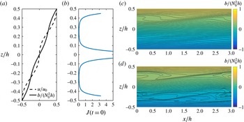
The initial mean profiles of buoyancy and velocity used in the DNS (a) and the corresponding gradient Richardson number (b). Vertical ( $x$ – $z$ ) slices of the buoyancy at time $t\simeq 52h/u_{0}$ show developing K–H billows and smaller-scale structures in the density field in the case with $Pr=7$ (d) compared with $Pr=0.7$ (c).

Initial profiles of velocity and buoyancy are shown in figure 1, along with the corresponding gradient Richardson number. Based on the Miles–Howard theorem, the flow has the capacity to support growing linear normal mode perturbations since $J<1/4$ in regions above and below the centreline. Overall, the disturbances to the linear velocity and buoyancy profile (and variations in the gradient Richardson number) are large. The framework described above, where small disturbances are considered, can be viewed as an analysis of a narrow range of $z_{\ast }$ . Kelvin–Helmholtz (K–H) billows develop in the weakly stratified regions, which distort the buoyancy contours (figure 1), with stronger distortion and smaller features in the $Pr=7$ simulation.

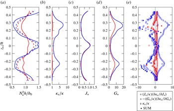
Interestingly, the initial disturbances to the stratification grow over time in the strongly stratified region near the centreline ( $z=0$ ) for $Pr=7$ but not when $Pr=0.7$ . Figure 2(a) shows profiles of $N_{\ast }^{2}$ for both simulations at $t\simeq 14h/u_{0}$ after decay of the initial random noise and at $t\simeq 105h/u_{0}$ , corresponding to a time after the first K–H mixing event. In the simulation with $Pr=7$ (blue), the stratification decreases in the regions that have $J<0.25$ at the start of the simulation, while the stratification intensifies near the centreline. In contrast, $N_{\ast }^{2}$ evolves towards a constant value in the simulation with $Pr=0.7$ (red).

Figure 2.

Vertical profiles in sorted buoyancy coordinates ( $z_{\ast }$ ) for simulations with $Pr=0.7$ (red) and $Pr=7$ (blue). (a) Normalized $N_{\ast }^{2}$ at $t\simeq 14h/u_{0}$ (dashed) and $t=105h/u_{0}$ (solid). (b) Normalized effective diffusivity, $\unicode[STIX]{x1D705}_{e}/\unicode[STIX]{x1D705}$ . (c) Gradient Richardson number, $J_{\ast }$ . (d) Buoyancy Reynolds number, $G_{\ast }$ . (e) Terms in (2.14), each normalized by  $\unicode[STIX]{x1D705}$ .

The amplification of the perturbations to the $N_{\ast }^{2}$ profile can be analysed using the theoretical framework introduced above. Profiles of $\unicode[STIX]{x1D705}_{e}$ , $J_{\ast }$ and $G_{\ast }$ at individual times are relatively noisy and intense mixing occurs in intermittent bursts. However, the general trends in each simulation can be seen by examining the time-averaged profiles. Figure 2(b) shows profiles of $\unicode[STIX]{x1D705}_{e}$ , normalized by the molecular value and averaged in the time interval bounded by the profiles shown in figure 2(a). The normalized effective diffusivity is larger in the case with $Pr=7$ . In both cases, $\unicode[STIX]{x2202}^{2}\unicode[STIX]{x1D705}_{e}/\unicode[STIX]{x2202}z_{\ast }^{2}<0$ in regions with relatively weak stratification and $\unicode[STIX]{x2202}^{2}\unicode[STIX]{x1D705}_{e}/\unicode[STIX]{x2202}z_{\ast }^{2}>0$ in regions with relatively strong stratification. This implies that the first term on the right-hand side of (2.3) will tend to reinforce perturbations to the $N_{\ast }^{2}$ profile. Time-averaged profiles of $J_{\ast }$ and $G_{\ast }$ are shown in figure 2(c,d). Regions with large $\unicode[STIX]{x1D705}_{e}$ are associated with small $J_{\ast }$ and large $G_{\ast }$ . Here, the profiles of $J_{\ast }(z_{\ast })$ and $G_{\ast }(z_{\ast })$ are very close to the profiles of the more conventional definitions in terms of unsorted height, $J(z)$ and $G(z)$ (not shown).

The terms in (2.14) are shown in figure 2(e), where each term is evaluated based on the time-averaged profiles of $\unicode[STIX]{x1D705}_{e}$ , $J_{\ast }$ and $G_{\ast }$ . Since the initial perturbations in the mean $J_{\ast }$ and $G_{\ast }$ profiles are not small, as assumed in obtaining (2.13), we have used the local values of $J_{\ast }$ and $G_{\ast }$ in evaluating (2.14), consistent with the interpretation that the framework applies to a small range of $z_{\ast }$ . The first two terms in (2.14) are generally negative and hence encourage negative diffusion and layer formation. On the other hand, as noted above, $\unicode[STIX]{x1D705}_{e}>0$ . When $Pr=0.7$ (red), $\unicode[STIX]{x1D705}_{e}$ is generally larger than the other terms, resulting in a positive diffusivity in (2.13). Although $\unicode[STIX]{x1D705}_{e}/\unicode[STIX]{x1D705}$ is larger for $Pr=7$ , the other terms more than compensate, and the condition in (2.14) is met at most locations. These results are consistent with the observation that changes in stratification intensify when $Pr=7$ , but not when $Pr=0.7$ .

Figure 2(e) includes the terms inside the bracket in (2.13) and hence determines whether the diffusion acting on $N_{1}$ is positive or negative. However, in this particular case, the last two terms in (2.13) are not negligible. Based on our initial conditions, $\unicode[STIX]{x2202}^{2}S_{\ast }/\unicode[STIX]{x2202}z_{\ast }^{2}$ has the opposite sign to $\unicode[STIX]{x2202}^{2}N_{\ast }^{2}/\unicode[STIX]{x2202}z_{\ast }^{2}$ . Similarly, as the simulation evolves, $\unicode[STIX]{x1D700}_{\ast }$ is large where $N_{\ast }^{2}$ is small and, although there are large fluctuations $\unicode[STIX]{x2202}^{2}\unicode[STIX]{x1D700}_{\ast }/\unicode[STIX]{x2202}z_{\ast }^{2}$ , generally has the opposite sign to $\unicode[STIX]{x2202}^{2}N_{\ast }^{2}/\unicode[STIX]{x2202}z_{\ast }^{2}$ . As a result, both terms encourage layer formation in our simulations.

Figure 3.

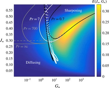
The irreversible mixing efficiency, $E(J_{\ast },G_{\ast })$ , as parameterized by Salehipour et al. (Reference Salehipour, Peltier, Whalen and MacKinnon2016) (colour shading). Solid contours separate regions where the bracketed term in (2.13) is sharpening and diffusive for four different values of the Prandtl (or Schmidt) number, $Pr=\unicode[STIX]{x1D708}/\unicode[STIX]{x1D705}$ . The dashed line delineates the region where $\unicode[STIX]{x2202}E/\unicode[STIX]{x2202}J_{\ast }=0$ . Mean profiles of $J_{\ast }$ and $G_{\ast }$ from the DNS (as plotted in figure 2) are shown using white dots for $Pr=7$ and black dots for $Pr=0.7$ .

4 Parameterizations

The previous section demonstrates that the framework developed in § 2 is useful for diagnosing the sharpening of a density profile though stratified turbulence. The framework can be applied more broadly by assuming a particular functional form for $\unicode[STIX]{x1D705}_{e}(J_{\ast },G_{\ast })$ . A simple expression follows if we assume that $\unicode[STIX]{x1D705}_{e}$ depends on $J_{\ast }$ and $G_{\ast }$ through a power law,

where $f(Pr,\ldots )$ includes the explicit dependence of $\unicode[STIX]{x1D705}_{e}$ on the Prandtl number and any other constant parameters. This form is unlikely to hold over a wide range of $J_{\ast }$ and $G_{\ast }$ for fixed values of $\unicode[STIX]{x1D6FC}$ and $\unicode[STIX]{x1D6FD}$ , but it might provide a reasonable approximation to $\unicode[STIX]{x1D705}_{e}$ for a limited range of $J_{\ast }$ and $G_{\ast }$ . The condition for a negative diffusivity in (2.14) then becomes simply

Based on DNS of homogeneous sheared stratified turbulence, Shih et al. (Reference Shih, Koseff, Ivey and Ferziger2005) found that the turbulent diffusivity increases with increasing $G$ with an exponent of $\unicode[STIX]{x1D6FD}\simeq 1$ for $7<G<100$ and $\unicode[STIX]{x1D6FD}\simeq 0.5$ for $G>100$ . (It should be noted that the turbulent diffusivity in Shih et al. (Reference Shih, Koseff, Ivey and Ferziger2005) is defined in terms of the buoyancy flux and buoyancy gradient in the vertical ( $z$ ) direction, while all quantities here are defined in terms of derivatives in sorted buoyancy coordinates,  $z_{\ast }$ .) Without additional dependence on the gradient Richardson number, this value of $\unicode[STIX]{x1D6FD}$ would not be sufficient for (2.14) to hold.

Recently, Salehipour et al. (Reference Salehipour, Peltier, Whalen and MacKinnon2016) collected data from DNS and developed a parameterization for the irreversible mixing efficiency, $E$ , as a function of the gradient Richardson and buoyancy Reynolds numbers in sorted buoyancy coordinates, $J_{\ast }$ and $G_{\ast }$ . Details of this parameterization can be found in Salehipour et al. (Reference Salehipour, Peltier, Whalen and MacKinnon2016). The colour shading in figure 3 shows the parameterized form of $E(G_{\ast },J_{\ast })$ , which notably has non-monotonic behaviour in both parameters. Solid contours separate regions where the condition in (2.16) holds for three different values of the Prandtl (or Schmidt) number, $Pr=0.7$ , 7, 700, corresponding approximately to the diffusion of heat in air, heat in water and salt in water. For reference, a line showing $Pr=\infty$ is also shown. There is non-trivial Prandtl and buoyancy Reynolds dependence on the condition in (2.16) with the parameterized form of $E(G_{\ast },J_{\ast })$ . The Prandtl number has a strong effect on the boundary for the range $J_{\ast }\gtrsim 0.25$ and $G_{\ast }\lesssim 100$ . Salehipour et al. (Reference Salehipour, Peltier, Whalen and MacKinnon2016) note that $E$ might depend explicitly on the Prandtl number, although they did not include this dependence in their parameterization.

The dashed line in figure 3 indicates where $\unicode[STIX]{x2202}E/\unicode[STIX]{x2202}J_{\ast }=0$ , and the region above this line satisfies $\unicode[STIX]{x2202}E/\unicode[STIX]{x2202}J_{\ast }<0$ . This gives a very good approximation to the full condition in (2.16) for $G_{\ast }>100$ . It should be noted, however, that the parameterized form of $E$ and the location where $\unicode[STIX]{x2202}E/\unicode[STIX]{x2202}J_{\ast }=0$ depend strongly on $G_{\ast }$ in this range.

The DNS results described in § 3 are qualitatively consistent with the sharpening criteria derived from the Salehipour et al. (Reference Salehipour, Peltier, Whalen and MacKinnon2016) parameterization. Black and white dots in figure 3 show individual points along the mean $J_{\ast }$ and $G_{\ast }$ profiles for $Pr=0.7$ (black) and $Pr=7$ (white). When $Pr=0.7$ , the values of $J_{\ast }$ and $G_{\ast }$ are always in the diffusing regime, while when $Pr=7$ , the profiles pass into the sharpening regime.